Symmetries, Reductions and Exact Solutions of a Class of (2k + 2)th-Order Difference Equations with Variable Coefficients

Abstract

We perform a Lie analysis of $(2k+2)$th-order difference equations and obtain $k+1$ non-trivial symmetries. We utilize these symmetries to obtain their exact solutions. Sufficient conditions for convergence of solutions are provided for some specific cases. We exemplify our theoretical analysis with some numerical examples. The results in this paper extend to some work in the recent literature.

1. Introduction

Rational ordinary difference equations have been studied in the literature by many researchers [1,2,3,4,5,6,7,8]. Recently, the well-known symmetry methods for differential equations have been extended to difference equations [9,10,11]. The concept is similar to the one developed for differential equations (see [12]), and it consists of solving the difference equations using the group of transformations that leave the equation invariant. Hydon [10] developed a systematic method that enables one to find the group of transformations for difference equations. Though his algorithm is valid for any given difference equation, he mainly applied it to second-order difference equations. This could be due to the fact that for higher-order difference equations, the calculations are cumbersome. For more references on recurrence equations via the symmetry approach, see [13,14,15].

In this paper, we investigate the solutions of difference equations of the form

$$\begin{array}{c}\hfill x_{n+1}=\frac{x_{n-(2k+1)}}{a_n+b_n{x}_{n-k}{x}_{n-(2k+1)}},\end{array}$$

(1)

for some arbitrary sequences $a_n$ and $b_n$ using a symmetry-based method.

Special cases of the above equation exist in the recent literature. In [1], Cinar studied the positive solutions of the special case where $a_n=1,b_n=1$, and $k=0$:

$$\begin{array}{c}\hfill x_{n+1}=\frac{x_{n-1}}{1+x_{n-1}{x}_n}.\end{array}$$

(2)

In [2], the author studied the special case where $a_n=-1,b_n=1$, and $k=0$:

$$\begin{array}{c}\hfill x_{n+1}=\frac{x_{n-1}}{-1+x_{n-1}{x}_n}.\end{array}$$

(3)

In [5], the author studied the special case where $a_n=1,b_n=a$, and $k=0$:

$$\begin{array}{c}\hfill x_{n+1}=\frac{x_{n-1}}{1+a{x}_{n-1}{x}_n}.\end{array}$$

(4)

In [4], the author studied the special case where $a_n=-1,b_n=a$, and $k=0$:

$$\begin{array}{c}\hfill x_{n+1}=\frac{x_{n-1}}{-1+a{x}_{n-1}{x}_n}.\end{array}$$

(5)

In [3], the author studied the special case where $a_n=1/a,b_n=b/a$, and $k=0$:

$$\begin{array}{c}\hfill x_{n+1}=\frac{a{x}_{n-1}}{1+b{x}_{n-1}{x}_n}.\end{array}$$

(6)

In [15], the author obtained the solutions of Equation (6) with less restrictions on the initial conditions.

In [6], the author studied the special case where $a_n=a,b_n=-1$, and $k=0$:

$$\begin{array}{c}\hfill x_{n+1}=\frac{x_{n-1}}{a-x_{n-1}{x}_n}.\end{array}$$

(7)

In [7], the case where $a_n=\pm 1,b_n=\pm 1$, and k = 1 such that

$$\begin{array}{c}\hfill x_{n+1}=\frac{x_{n-3}}{\pm 1\pm x_{n-1}{x}_{n-3}},\end{array}$$

(8)

was studied by Elsayed, and exact solutions were obtained.

In [8], the author studied and obtained exact solutions of the special case where $a_n=-1,b_n=1$, and $k=2$:

$$\begin{array}{c}\hfill x_{n+1}=\frac{x_{n-5}}{-1+x_{n-3}{x}_{n-5}}.\end{array}$$

(9)

In [16], the author studied the positive solutions and attractivenesss of the special case where $a_n=1$ and $b_n=1$:

$$\begin{array}{c}\hfill x_{n+1}=\frac{x_{n-(2k+1)}}{1+x_{n-k}{x}_{n-(2k+1)}}.\end{array}$$

(10)

In [17], the author studied the solutions of the special case where $a_n=-1$ and $b_n=1/a$:

$$\begin{array}{c}\hfill x_{n+1}=\frac{a{x}_{n-(2k+1)}}{-a+x_{n-k}{x}_{n-(2k+1)}}.\end{array}$$

(11)

For more work on difference equations, please see [18].

For definiteness, we study the difference equation

$$\begin{array}{c}\hfill u_{n+2k+2}=\frac{u_n}{A_n+B_n{u}_{n+k+1}{u}_n},\end{array}$$

(12)

instead of Equation (1). To derive the solutions for Equation (12) using a symmetry-based method, we will first find the Lie group of point transformations of Equation (12). Then, we will reduce the order via the invariants and construct the solutions. Furthermore, we will explain how the solutions for Equation (1) can be obtained from the solutions for Equation (12). Finally, we will show how one can obtain the results in the literature using our results.

Preliminaries

In this section, we provide background to Lie symmetry analysis of difference equations. In this paper, we adopt the same notation as that in [10].

Definition 1.

Let G be a local group of transformations acting on a manifold M. A subset $\mathcal{S}\subset M$ is called G-invariant, and G is called a symmetry group of $\mathcal{S}$. If whenever $x\in \mathcal{S}$, and $g\in G$ is such that $g·x$ is defined, then $g·x\in \mathcal{S}$ [12].

Definition 2.

Let G be a connected group of transformations acting on a manifold M. A smooth real-valued function $\zeta :M\to \mathbb{R}$ is an invariant function for G if and only if

$$X\left(\zeta \right)=0forallx\in M,$$

and every infinitesimal generator X of G [12].

Definition 3.

A parameterized set of point transformations

$${\Gamma }_{\epsilon }:x\mapsto \widehat{x}(x;\epsilon ),$$

where $x=x_i,$$i=1,\cdots ,p$ are continuous variables is a one-parameter local Lie group of transformations if the following conditions are satisfied [10]:

• ${\Gamma }_0$ is the identity map if $\widehat{x}=x$ when $\epsilon =0$;
• ${\Gamma }_a{\Gamma }_b={\Gamma }_{a+b}$ for every a and b sufficiently close to 0;
• Each $\widehat{x_i}$ can be represented as a Taylor series (in a neighborhood of $\epsilon =0$ that is determined by x), and therefore

$$\widehat{x_i}(x:\epsilon )=x_i+\epsilon {\xi }_i\left(x\right)+O\left({\epsilon }^2\right),i=1,\dots ,p.$$

Consider the ordinary difference equation

$$u_{n+2k+2}=\omega (n,u_n,u_{n+1},\cdots ,u_{n+2k+1}),n\in D$$

(13)

for some smooth function $\omega$ and a regular domain $D\subset \mathbb{Z}$. To find a symmetry group of Equation (13), we consider the group of point transformations given by

$$G_{\epsilon }:(n,u_n)\mapsto (n,u_n+\epsilon Q(n,u_n)),$$

(14)

where $\epsilon$ is the parameter and Q is a continuous function which we shall refer to as a characteristic. Let

$$\begin{array}{cc}\hfill X=& Q(n,u_n)\frac{\partial }{\partial u_n}+Q(n+1,u_{n+1})\frac{\partial }{\partial u_{n+1}}+Q(n+2,u_{n+2})\frac{\partial }{\partial u_{n+2}}+\cdots \hfill \\ \hfill & \cdots +Q(n+2k+1,u_{n+2k+1})\frac{\partial }{\partial u_{n+2k+1}}\hfill \end{array}$$

be the corresponding infinitesimal of $G_{\epsilon }$. The substitution of the new variable (obtained using $G_{\epsilon }$ given in Equation (14)) in Equation (13) yields the linearized symmetry condition

$${\mathcal{S}}^{(2k+2)}Q(n,u_n)-X\omega =0$$

(15)

whenever Equation (13) is true. The shift operator S acts on n as follows: $S:n\to n+1$. Once the characteristic $Q=Q(n,u_n)$ is known, the invariant $V_n$ may be obtained by solving the characteristic system [12]

$$\frac{d{u}_n}{Q}=\frac{d{u}_{n+1}}{SQ}=\cdots =\frac{d{u}_{n+2k+1}}{S^{n+2k+1}Q}\left(=\frac{d{V}_n}{0}\right)$$

or by introducing the canonical coordinate [19]

$$\begin{array}{c}\hfill s_n=\int \frac{d{u}_n}{Q(n,u_n)}.\end{array}$$

We use the standard conventions

$$\begin{array}{c}\hfill \prod _{j=s}^l{\theta }_j=1\mathrm{when}s>l\mathrm{and}\sum _{j=s}^l{\theta }_j=0\mathrm{when}s>l.\end{array}$$

2. Symmetries

Consider the $(2k+2)$th-order difference Equation (12), which is

$$\begin{array}{c}\hfill u_{n+2k+2}=\frac{u_n}{A_n+B_n{u}_{n+k+1}{u}_n}.\end{array}$$

To obtain the symmetries, we impose the infinitesimal criterion of invariance (Equation (15)) to obtain

$$\begin{array}{c}\hfill \begin{array}{cc}\hfill & Q(n+2k+2,u_{n+2k+2})+\frac{B_n{u_n}^2}{{(B_n{u}_n{u}_{n+k+1}+A_n)}^2}Q(n+k+1,u_{n+k+1})\hfill \\ \hfill & -\frac{A_n}{{(B_n{u}_n{u}_{n+k+1}+A_n)}^2}Q(n,u_n)=0.\hfill \end{array}\end{array}$$

(16)

The latter is a functional equation for the characteristic Q, making Equation (16) difficult to solve. To eliminate the first undesirable argument $u_{n+2k+2}$, we differentiate implicitly with respect to $u_n$ (keeping $u_{n+2k+2}$ fixed and regarding $u_{n+k+1}$ as a function of $u_n$ and $u_{n+2k+2}$). This leads to

$$\begin{array}{cc}\hfill & \frac{1}{{(B_n{u}_n{u}_{n+k+1}+A_n)}^2}\frac{\partial }{\partial u_{n+k+1}}Q(n+k+1,u_{n+k+1})-\hfill \\ \hfill & \frac{1}{{(B_n{u}_n{u}_{n+k+1}+A_n)}^2}\frac{\partial }{\partial u_n}Q(n,u_n)+\frac{2}{u_n{(B_n{u}_n{u}_{n+k+1}+A_n)}^2}Q(n,u_n)=0\hfill \end{array}$$

After simplification, we obtain

$$\begin{array}{c}\hfill \frac{\partial }{\partial u_{n+k+1}}Q(n+k+1,u_{n+k+1})-\frac{\partial }{\partial u_n}Q(n,u_n)+\frac{2}{u_n}Q(n,u_n)=0.\end{array}$$

To eliminate the second undesirable variable $u_{n+k+1}$, we differentiate with respect to $u_n$, and we obtain the following second-order differential equation involving only the argument $u_n$:

$$\begin{array}{c}\hfill \frac{{\mathrm{d}}^2}{\mathrm{d}{u_n}^2}Q(n,u_n)-\frac{2}{u_n}\frac{\mathrm{d}}{\mathrm{d}{u}_n}Q(n,u_n)+\frac{2}{{u_n}^2}Q(n,u_n)=0.\end{array}$$

(17)

The general solution of Equaiton (17) is then given by

$$\begin{array}{c}\hfill Q=f\left(n\right)u_n+g\left(n\right){u_n}^2,\end{array}$$

(18)

where f and g are arbitrary functions of n. To eliminate the dependency between these two functions, we substitute Equation (18) into Equation (16) and simplify the resulting equation to obtain

$$\begin{array}{cc}\hfill & B_{n}g\left(n+k+1\right){u_{n+k+1}}^2{u_n}^2+B_{n}f\left(n+k+1\right)u_{n+k+1}{u_n}^2+B_{n}f\left(n+2k+2\right)u_{n+k+1}{u_n}^2\hfill \\ \hfill & -A_{n}g\left(n\right){u_n}^2-A_{n}f\left(n\right)u_n+A_{n}f\left(n+2k+2\right)u_n+g\left(n+2k+2\right){u_n}^2=0.\hfill \end{array}$$

We separate by powers of shifts of $u_n$, and we readily reduce the resulting over-determining system to obtain

$$\begin{array}{cc}\hfill & f\left(n\right)+f\left(n+k+1\right)=0,\hfill \\ \hfill & g\left(n\right)=0.\hfill \end{array}$$

(19)

The solutions for Equation (19) are

$$\begin{array}{c}\hfill \left\{\begin{array}{cc}\hfill & exp\left[\pm i\left(\frac{(2s+1)n\pi }{k+1}\right)\right],0\le s\le (k-1)/2\mathrm{if}k\mathrm{odd}\hfill \\ & \\ \hfill & {(-1)}^n,exp\left[\pm i\left(\frac{(2s+1)n\pi }{k+1}\right)\right],0\le s\le (k-2)/2\mathrm{if}k\mathrm{even}.\hfill \end{array}\right.\end{array}$$

This means that we have $k+1$ non-trivial characteristics

$$\begin{array}{cc}\hfill Q_s=& {\left({\beta }_s\right)}^n{u}_n,\hfill \\ \hfill {\widehat{Q}}_s=& {\left({\overline{\beta }}_s\right)}^n{u}_n,0\le s\le \frac{k-1}{2}\mathrm{if}k\mathrm{odd}\hfill \end{array}$$

and

$$\begin{array}{cc}\hfill Q_{-1}=& {(-1)}^n{u}_n,\hfill \\ \hfill Q_s=& {\left({\beta }_s\right)}^n{u}_n,\hfill \\ \hfill {\widehat{Q}}_s=& {\left({\overline{\beta }}_s\right)}^n{u}_n,0\le s\le \frac{k-2}{2}\mathrm{if}k\mathrm{even},\hfill \end{array}$$

where ${\beta }_s=exp\left[i\left(\frac{(2s+1)\pi }{k+1}\right)\right]$. We will refer to $X_i$ as the corresponding symmetry generator of $Q_i$.

3. Exact Solutions

Here, we introduce the canonical coordinate (i.e., the variable $S_n$ such that $X{S}_n=1$). We use the well-known choice [19]

$$\begin{array}{c}\hfill S_n=\int \frac{d{u}_n}{Q(n,u_n)}.\end{array}$$

Using any one of the symmetry generators, such as $X_s$, we have that

$$\begin{array}{c}\hfill S_n=\int \frac{d{u}_n}{Q_s(n,u_n)}=\frac{1}{{\left({\beta }_s\right)}^n}ln\left|u_n\right|.\end{array}$$

Using Equation (19), we have proven that

$$\begin{array}{c}\hfill X_s\left[{\left({\beta }_s\right)}^{n+k+1}{S}_{n+k+1}+{\left({\beta }_s\right)}^n{S}_n\right]=0\end{array}$$

(20)

Therefore, the following is an invariant function of $X_s$:

$$\begin{array}{c}\hfill r_n={\left({\beta }_s\right)}^{n+k+1}{S}_{n+k+1}+{\left({\beta }_s\right)}^n{S}_n\end{array}$$

Since the equation under study is a rational difference equation, it is favorable to use

$$\begin{array}{c}\hfill |{\tilde{r}}_n|=exp(-r_n),\end{array}$$

(21)

In other words, ${\tilde{r}}_n=\pm 1/u_n{u}_{n+k+1}$. It turns out (using the plus sign together with Equation (12)) that

$$\begin{array}{c}\hfill {\tilde{r}}_{n+k+1}=A_n{\tilde{r}}_n+B_n.\end{array}$$

(22)

It is easy to verify that the solution for Equation (22) in closed form is given by

$$\begin{array}{c}\hfill {\tilde{r}}_{(k+1)n+j}={\tilde{r}}_j\left(\prod _{k_1=0}^{n-1}{A}_{(k+1)k_1+j}\right)+\sum _{l=0}^{n-1}\left(B_{(k+1)l+j}\prod _{k_2=l+1}^{n-1}{A}_{(k+1)k_2+j}\right),\end{array}$$

(23)

for $j=0,1,\cdots ,k$. By going up the hierarchy created by the change of variables, we obtain the solution for Equation (12) in a unified manner as follows:

• For k being odd:

  $$\begin{array}{cc}\hfill |u_n|=& exp\{\sum _{s=0}^{\frac{k-1}{2}}\left(c_s{{\beta }_s}^n+{\tilde{c}}_s{{\overline{\beta }}_s}^n\right)+\sum _{s=0}^{\frac{k-1}{2}}\left(\sum _{k_s=0}^{n-1}\frac{1}{k+1}{{\beta }_s}^n{{\overline{\beta }}_s}^{k_s}ln{\tilde{r}}_{k_s}\right)\hfill \\ \hfill & +\sum _{s=0}^{\frac{k-1}{2}}\left(\sum _{k_s=0}^{n-1}\frac{1}{k+1}{\overline{{\beta }_s}}^n{{\beta }_s}^{k_s}ln{\tilde{r}}_{k_s}\right)\}\hfill \\ \hfill |u_n|=& {\Gamma }_{n}exp\left\{\sum _{s=0}^{\frac{k-1}{2}}\left(\sum _{k_s=0}^{n-1}\frac{2}{k+1}\mathrm{Re}\left[{\gamma }_s(n,k_s)\right]ln{\tilde{r}}_{k_s}\right)\right\}\hfill \end{array}$$

  (24)
• For k being even:

  $$\begin{array}{c}\hfill \begin{array}{cc}|u_n|=& {\theta }_{n}exp\{{\displaystyle \sum _{s=0}^{\frac{k-2}{2}}}\left({\displaystyle \sum _{k_s=0}^{n-1}}\frac{2}{k+1}\mathrm{Re}\left[{\gamma }_s(n,k_s)\right]ln{\tilde{r}}_{k_s}\right)\\ & +{(-1)}^n\sum _{j=0}^{n-1}\frac{1}{k+1}{(-1)}^{j}ln{\tilde{r}}_{(k+1)}j\}\end{array}\end{array}$$

  (25)

where

$$\begin{array}{cc}\hfill & {\Gamma }_n=exp\left[\sum _{s=0}^{\frac{k-1}{2}}\left(c_s{{\beta }_s}^n+{\tilde{c}}_s{{\overline{\beta }}_s}^n\right)\right],\hfill \\ \hfill & {\theta }_n=exp\left[c{(-1)}^n+\sum _{s=0}^{\frac{k-2}{2}}\left(c_s{{\beta }_s}^n+{\tilde{c}}_s{{\overline{\beta }}_s}^n\right)\right],\hfill \\ \hfill & {\gamma }_s(n,k_s)={{\beta }_s}^n{{\overline{\beta }}_s}^{k_s}.\hfill \end{array}$$

The properties of ${\Gamma }_n,{\theta }_n$ and $\gamma (n,k)$ are as follows:

$$\begin{array}{cc}\hfill & {\Gamma }_{(2k+2)n+j}={\Gamma }_j=\left|u_j\right|,0\le j\le k\hfill \\ \hfill & {\Gamma }_{(2k+2)n+k+1+j}=\frac{1}{{\Gamma }_j}=\frac{1}{|u_j|},0\le j\le k\hfill \end{array}$$

$$\begin{array}{cc}\hfill & {\theta }_{(2k+2)n+j}={\theta }_j=\left|u_j\right|,0\le j\le k\hfill \\ \hfill & {\theta }_{(2k+2)n+k+1+j}=\frac{1}{{\theta }_j}=\frac{1}{|u_j|},0\le j\le k\hfill \end{array}$$

$$\begin{array}{cc}\hfill & {\gamma }_s((2k+2)n,j)={\gamma }_s(0,j),\hfill \\ \hfill & {\gamma }_s(n+k+1,j)={\gamma }_s(n,j+k+1)=-{\gamma }_s(n,j),\hfill \\ \hfill & {\gamma }_s(j,j)=1.\hfill \end{array}$$

In regard to these properties, one can further simplify the solution through Equations (24) and (25). We have that

$$\begin{array}{cc}\hfill |u_{(2k+2)n}|=& {\Gamma }_{(2k+2)n}exp\left\{\sum _{s=0}^{\frac{k-1}{2}}\left(\sum _{k_s=0}^{(2k+2)n-1}\frac{2}{k+1}\mathrm{Re}\left[{\gamma }_s((2k+2)n,k_s)\right]ln{\tilde{r}}_{k_s}\right)\right\}\hfill \\ \hfill =& u_{0}exp\left\{\sum _{s=0}^{\frac{k-1}{2}}\left(\sum _{k_s=0}^{(2k+2)n-1}\frac{2}{k+1}\mathrm{Re}\left[{\gamma }_s(0,k_s)\right]ln{\tilde{r}}_{k_s}\right)\right\}\hfill \\ \hfill =& u_{0}exp\left\{\frac{2}{k+1}\sum _{k_0=0}^{(2k+2)n-1}\mathrm{Re}\right[exp\left(-\frac{k_0}{k+1}i\pi \right)+exp\left(-\frac{3k_0}{k+1}i\pi \right)\hfill \\ \hfill & +\cdots +exp\left(-\frac{k{k}_0}{k+1}i\pi \right)]ln{\tilde{r}}_{k_0}\}\hfill \\ \hfill =& u_{0}exp\left\{\frac{2}{k+1}\sum _{k_0=0}^{2n-1}\mathrm{Re}\right[exp\left(-k_{0}i\pi \right)+exp\left(-3k_{0}i\pi \right)+\cdots \hfill \\ & +exp\left(-k{k}_{0}i\pi \right)]ln{\tilde{r}}_{k_0}\}\hfill \\ \hfill =& u_{0}exp\left\{\sum _{k_0=0}^{2n-1}{(-1)}^{k_0}ln{\tilde{r}}_{k_0(k+1)}\right\}\hfill \\ \hfill =& \left|u_0\prod _{k_0=0}^{n-1}\frac{{\tilde{r}}_{2k_0(k+1)}}{{\tilde{r}}_{(2k_0+1)(k+1)}}\right|.\hfill \end{array}$$

(26)

Note: It can be shown, using the expression of ${\tilde{r}}_n$ given in Equation (21), that one can write Equation (26) without using the symbol of the absolute value.

On this note, and in the same way, we have proven that

$$\begin{array}{cc}\hfill u_{(2k+2)n+j}=& u_j\prod _{k_0=0}^{n-1}\frac{{\tilde{r}}_{2k_0(k+1)+j}}{{\tilde{r}}_{(2k_0+1)(k+1)+j}},0\le j\le k,\hfill \end{array}$$

(27)

$$\begin{array}{cc}\hfill u_{(2k+2)n+k+1+j}=& u_{k+1+j}\prod _{k_0=0}^{n-1}\frac{{\tilde{r}}_{(2k_0+1)(k+1)+j}}{{\tilde{r}}_{(2k_0+2)(k+1)+j}},0\le j\le k.\hfill \end{array}$$

(28)

We therefore obtain, by combining Equations (23), (27) and (28) and by replacing ${\tilde{r}}_i$ with $1/\left(u_i{u}_{i+k+1}\right)$, the solution for Equation (12) in closed form as

$$\begin{array}{c}\hfill \begin{array}{cc}\hfill & u_{(2k+2)n+j}=\hfill \\ \hfill & u_j\prod _{k_0=0}^{n-1}\frac{\left({\displaystyle \prod _{k_1=0}^{2k_0-1}}{A}_{(k+1)k_1+j}\right)+u_j{u}_{j+k+1}{\displaystyle \sum _{l=0}^{2k_0-1}}\left(B_{(k+1)l+j}{\displaystyle \prod _{k_2=l+1}^{2k_0-1}}{A}_{(k+1)k_2+j}\right)}{\left({\displaystyle \prod _{k_1=0}^{2k_0}}{A}_{(k+1)k_1+j}\right)+u_j{u}_{j+k+1}{\displaystyle \sum _{l=0}^{2k_0}}\left(B_{(k+1)l+j}{\displaystyle \prod _{k_2=l+1}^{2k_0}}{A}_{(k+1)k_2+j}\right)},\hfill \end{array}\end{array}$$

(29)

$$\begin{array}{c}\hfill \begin{array}{cc}\hfill & u_{(2k+2)n+k+1+j}=\hfill \\ \hfill & u_{k+1+j}\prod _{k_0=0}^{n-1}\frac{\left({\displaystyle \prod _{k_1=0}^{2k_0}}{A}_{(k+1)k_1+j}\right)+u_j{u}_{j+k+1}{\displaystyle \sum _{l=0}^{2k_0}}\left(B_{(k+1)l+j}{\displaystyle \prod _{k_2=l+1}^{2k_0}}{A}_{(k+1)k_2+j}\right)}{\left({\displaystyle \prod _{k_1=0}^{2k_0+1}}{A}_{(k+1)k_1+j}\right)+u_j{u}_{j+k+1}{\displaystyle \sum _{l=0}^{2k_0+1}}\left(B_{(k+1)l+j}{\displaystyle \prod _{k_2=l+1}^{2k_0+1}}{A}_{(k+1)k_2+j}\right)},\hfill \end{array}\end{array}$$

(30)

where $0\le j\le k$ and provided that

$$\begin{array}{c}\hfill -u_j{u}_{j+k+1}\sum _{l=0}^m\left(B_{(k+1)l+j}\prod _{k_2=l+1}^m{A}_{(k+1)k_2+j}\right)\ne \prod _{k_1=0}^m{A}_{(k+1)k_1+j},\end{array}$$

(31)

where $m<2n$. Recall that we enacted the shift operator $2k+1$ times in Equation (1) to obtain Equation (12), and therefore we can write the solutions for Equation (1) as follows

$$\begin{array}{cc}\hfill & x_{(2k+2)n-(2k+1)+j}=\hfill \\ & x_{j-2k-1}\prod _{k_0=0}^{n-1}\frac{\left({\displaystyle \prod _{k_1=0}^{2k_0-1}}{a}_{(k+1)k_1+j}\right)+x_{j-2k-1}{x}_{j-k}{\displaystyle \sum _{l=0}^{2k_0-1}}\left(b_{(k+1)l+j}{\displaystyle \prod _{k_2=l+1}^{2k_0-1}}{a}_{(k+1)k_2+j}\right)}{\left({\displaystyle \prod _{k_1=0}^{2k_0}}{a}_{(k+1)k_1+j}\right)+x_{j-2k-1}{x}_{j-k}{\displaystyle \sum _{l=0}^{2k_0}}\left(b_{(k+1)l+j}{\displaystyle \prod _{k_2=l+1}^{2k_0}}{a}_{(k+1)k_2+j}\right)},\hfill \end{array}$$

(32)

$$\begin{array}{cc}\hfill & x_{(2k+2)n-k+j}=\hfill \\ & x_{j-k}\prod _{k_0=0}^{n-1}\frac{\left({\displaystyle \prod _{k_1=0}^{2k_0}}{a}_{(k+1)k_1+j}\right)+x_{j-2k-1}{x}_{j-k}{\displaystyle {\displaystyle \sum _{l=0}^{2k_0}}}\left(b_{(k+1)l+j}{\displaystyle \prod _{k_2=l+1}^{2k_0}}{a}_{(k+1)k_2+j}\right)}{\left({\displaystyle \prod _{k_1=0}^{2k_0+1}}{a}_{(k+1)k_1+j}\right)+x_{j-2k-1}{x}_{j-k}{\displaystyle \sum _{l=0}^{2k_0+1}}\left(b_{(k+1)l+j}{\displaystyle \prod _{k_2=l+1}^{2k_0+1}}{a}_{(k+1)k_2+j}\right)},\hfill \end{array}$$

(33)

provided that

$$\begin{array}{c}\hfill -x_{j-2k-1}{x}_{j-k}\sum _{l=0}^m\left(b_{(k+1)l+j}\prod _{k_2=l+1}^m{a}_{(k+1)k_2+j}\right)\ne \prod _{k_1=0}^m{a}_{(k+1)k_1+j},m<2n.\end{array}$$

(34)

3.1. Case with $(K+1)$-Periodic Sequences $\left(A_n\right)$ and $\left(B_n\right)$

Let $\left(a_n\right)=(a_0,a_1,\cdots ,a_k,a_0,a_1,\cdots )$, $\left(b_n\right)=(b_0,b_1,\cdots ,b_k,b_0,b_1,\cdots )$ and ${\Phi }_j=x_{j-2k-1}{x}_{j-k}{b}_j$. The solutions given in Equations (32), (33) and (34) simplify to

$$\begin{array}{cc}\hfill x_{(2k+2)n+j-(2k+1)}=& x_{j-2k-1}\prod _{k_0=0}^{n-1}\frac{{\left(a_j\right)}^{2k_0}+{\Phi }_j{\displaystyle \sum _{l=0}^{2k_0-1}}{\left(a_j\right)}^l}{{\left(a_j\right)}^{2k_0+1}+{\Phi }_j{\displaystyle \sum _{l=0}^{2k_0}}{\left(a_j\right)}^l},\hfill \end{array}$$

(35)

$$\begin{array}{cc}\hfill x_{(2k+2)n-k+j}=& x_{j-k}{\displaystyle \prod _{k_0=0}^{n-1}}\frac{{\left(a_j\right)}^{2k_0+1}+{\Phi }_j{\displaystyle \sum _{l=0}^{2k_0}}{\left(a_j\right)}^l}{{\left(a_j\right)}^{2k_0+2}+{\Phi }_j{\displaystyle \sum _{l=0}^{2k_0+1}}{\left(a_j\right)}^l},\hfill \end{array}$$

(36)

with

$$\begin{array}{c}\hfill {\Phi }_j\sum _{l=0}^{2k_0}{\left(a_j\right)}^l\ne -{\left(a_j\right)}^{2k_0+1},k_0<n,{\Phi }_j\sum _{l=0}^{2k_0+1}{\left(a_j\right)}^l\ne -{\left(a_j\right)}^{2k_0+2},k_0<n,j\le k.\end{array}$$

(37)

Case with $A_j\ne 1$

The solutions given in (35), (36) and (37) become

$$\begin{array}{cc}\hfill x_{(2k+2)n+j-(2k+1)}=& x_{j-2k-1}\prod _{k_0=0}^{n-1}\frac{{\left(a_j\right)}^{2k_0}+{\Phi }_j\left(\frac{1-{\left(a_j\right)}^{2k_0}}{1-a_j}\right)}{{\left(a_j\right)}^{2k_0+1}+{\Phi }_j\left(\frac{1-{\left(a_j\right)}^{2k_0+1}}{1-a_j}\right)}\hfill \end{array}$$

(38)

$$\begin{array}{cc}\hfill x_{(2k+2)n-k+j}=& x_{j-k}\prod _{k_0=0}^{n-1}\frac{{\left(a_j\right)}^{2k_0+1}+{\Phi }_j\left(\frac{1-{\left(a_j\right)}^{2k_0+1}}{1-a_j}\right)}{{\left(a_j\right)}^{2k_0+2}+{\Phi }_j\left(\frac{1-{\left(a_j\right)}^{2k_0+2}}{1-a_j}\right)},\hfill \end{array}$$

(39)

with

$$\begin{array}{cc}\hfill & {\Phi }_j\left(1-{\left(a_j\right)}^{2k_0+1}\right)\ne -\left(1-a_j\right){\left(a_j\right)}^{2k_0+1},\hfill \end{array}$$

(40)

$$\begin{array}{c}\hfill {\Phi }_j\left(1-{\left(a_j\right)}^{2k_0+2}\right)\ne -\left(1-a_j\right){\left(a_j\right)}^{2k_0+2},k_0<n,j\le k.\end{array}$$

(41)

3.2. Case with One-Periodic Sequences $\left(A_n\right)$ and $\left(B_n\right)$

Let $\left(a_n\right)=(a_0,a_0,\cdots )$, $\left(b_n\right)=(b_0,b_0,\cdots )$ and ${\Phi }_j=x_{j-2k-1}{x}_{j-k}{b}_0$. The solutions given in Equations (35), (36) and (37) simplify to

$$\begin{array}{cc}\hfill x_{(2k+2)n+j-(2k+1)}=& x_{j-2k-1}{\displaystyle \prod _{k_0=0}^{n-1}}\frac{{\left(a_0\right)}^{2k_0}+{\Phi }_j{\displaystyle \sum _{l=0}^{2k_0-1}}{\left(a_0\right)}^l}{{\left(a_0\right)}^{2k_0+1}+{\Phi }_j{\displaystyle \sum _{l=0}^{2k_0}}{\left(a_0\right)}^l}\hfill \end{array}$$

(42)

$$\begin{array}{cc}\hfill x_{(2k+2)n-k+j}=& x_{j-k}{\displaystyle \prod _{k_0=0}^{n-1}}\frac{{\left(a_0\right)}^{2k_0+1}+{\Phi }_j{\displaystyle \sum _{l=0}^{2k_0}}{\left(a_0\right)}^l}{{\left(a_0\right)}^{2k_0+2}+{\Phi }_j{\displaystyle \sum _{l=0}^{2k_0+1}}{\left(a_0\right)}^l},\hfill \end{array}$$

(43)

with

$$\begin{array}{c}\hfill {\Phi }_j\sum _{l=0}^{2k_0}{\left(a_0\right)}^l\ne -{\left(a_0\right)}^{2k_0+1},{\Phi }_j\sum _{l=0}^{2k_0+1}{\left(a_0\right)}^l\ne -{\left(a_0\right)}^{2k_0+2},k_0<n,j\le k.\end{array}$$

(44)

3.2.1. Case with $A_0\ne 1$

The solutions given in Equations (42), (43) and (44) become

$$\begin{array}{cc}\hfill x_{(2k+2)n+j-(2k+1)}=& x_{j-2k-1}\prod _{k_0=0}^{n-1}\frac{{\left(a_0\right)}^{2k_0}+{\Phi }_j\left(\frac{1-{\left(a_0\right)}^{2k_0}}{1-a_0}\right)}{{\left(a_0\right)}^{2k_0+1}+{\Phi }_j\left(\frac{1-{\left(a_0\right)}^{2k_0+1}}{1-a_0}\right)}\hfill \end{array}$$

(45)

$$\begin{array}{cc}\hfill x_{(2k+2)n-k+j}=& x_{j-k}\prod _{k_0=0}^{n-1}\frac{{\left(a_0\right)}^{2k_0+1}+{\Phi }_j\left(\frac{1-{\left(a_0\right)}^{2k_0+1}}{1-a_0}\right)}{{\left(a_0\right)}^{2k_0+2}+{\Phi }_j\left(\frac{1-{\left(a_0\right)}^{2k_0+2}}{1-a_0}\right)},\hfill \end{array}$$

(46)

with

$$\begin{array}{c}\hfill {\Phi }_j\left(1-{\left(a_0\right)}^{2k_0+1}\right)\ne -\left(1-a_0\right){\left(a_0\right)}^{2k_0+1},{\Phi }_j\left(1-{\left(a_0\right)}^{2k_0+2}\right)\ne -\left(1-a_0\right){\left(a_0\right)}^{2k_0+2},\end{array}$$

(47)

$k_0<n,j\le k.$

3.2.2. Case with $A_0=1$

The solutions given in Equations (42), (43) and (44) become

$$\begin{array}{cc}\hfill x_{(2k+2)n+j-(2k+1)}=& x_{j-2k-1}\prod _{k_0=0}^{n-1}\frac{1+\left(2k_0\right){\Phi }_j}{1+(2k_0+1){\Phi }_j}\hfill \end{array}$$

(48)

$$\begin{array}{cc}\hfill x_{(2k+2)n-k+j}=& x_{j-k}\prod _{k_0=0}^{n-1}\frac{1+(2k_0+1){\Phi }_j}{1+(2k_0+2){\Phi }_j},\hfill \end{array}$$

(49)

with

$$\begin{array}{c}\hfill (2k_0+1){\Phi }_j\ne -1,(2k_0+2){\Phi }_j\ne -1,k_0<n,j\le k.\end{array}$$

(50)

4. Results

In this section, we verify the results in [1,2,3,4,5,6,7,8,16,17] by utilizing different combinations of values of $a_n$ and $b_n$ in Equation (1):

• If we set $k=0,b_0=1$ in Equations (42)–(44), we obtain the result in [1] (see Theorem 2.1) for Equation (2). However, the restriction ($x_{-1}$ and $x_0$ are positive real numbers) in [1] is a special case of our restrictions ($(2k_0+1)x_{-1}{x}_0\ne -1$ and $(2k_0+1)x_0{x}_1\ne -1,k_0<n$);
• If we set $k=0,b_0=1$ in Equations (45)–(47), we obtain the result in [2] for Equation (3) (see Theorem 2.1). The restriction ($x_{-1}{x}_0\ne 1$) in [2] coincides with our restriction;
• If we set $k=0,b_0=a$ in Equations (48)–(50), we obtain the result in [5] for Equation (4) (see Theorem 2.1). However, the restriction ($x_{-1}$ and $x_0$ are nonnegative real numbers) in [5] is a special case of our restrictions ($(2k_0+1)a{x}_{-1}{x}_0\ne -1$ and $(2k_0+2)a{x}_{-1}{x}_0\ne -1,k_0<n$);
• If we set $k=0$ and $b_0=a$ in Equations (45)–(47), we obtain the result in [4] for Equation (5) (see Theorem 2.1), and the restriction ($a{x}_{-1}{x}_0\ne 1$) in [4] coincides with our restriction;
• If we set $k=0,a_0=(1/a)$, and $b_0=(b/a)$ in Equations (42)–(44) we obtain the result in [3] for Equation (6) (see Theorem 2.1). However, the restriction ($a,b,x_{-1}$, and $x_0$ are nonnegative real numbers) in [3] is a special case of our restrictions ($b{x}_{-1}{x}_0{\displaystyle \sum _{l=0}^{2k_0}}{a}^l\ne -1$ and $b{x}_{-1}{x}_0{\displaystyle \sum _{l=0}^{2k_0+1}}{a}^l\ne -1,k_0<n$);
• If we set $k=0,a_0=a$, and $b_0=-1$ in Equations (42)–(44), we obtain the result (for the case $a\ne 1$) in [6] for Equation (7) (see Theorem 2), and the restriction ($x_{-1}{x}_0\ne a^j(1-a)/(1-a^j)$) in [6] coincides with our restrictions ($x_{-1}{x}_0\left(1-a^{2k_0+1}\right)\ne$$\left(1-a\right)a^{2k_0+1}$, $x_{-1}{x}_0\left(1-a^{2k_0+2}\right)\ne \left(1-a\right)a^{2k_0+2}$, and $k_0<n$). Additionally, the solution for the case $a=1$ (see Theorem 5 in [6]) corresponds to our solution with the same restrictions on the initial conditions;
• If we set $k=1,a_0=1$, and $b_0=1$ (resp $b_0=-1$) in Equations (48)–(50), we obtain the result in [7] for Equation (8) (see Theorem 1 (resp. Theorem 4)). However, the restriction ($x_{-1}$ and $x_0$ are nonzero positive real numbers (resp. $j{x}_0{x}_{-2}\ne 1$, $j{x}_{-1}{x}_{-3}\ne 1$ for $j=1,2,3,\cdots$)) in [7] is a special case of our restrictions ($(2k_0+1)x_{-1}{x}_{-3}\ne -1,(2k_0+2)x_0{x}_{-2}\ne -1$ (resp. $[2k_0+1]x_{-1}{x}_{-3}\ne 1$, and $[2k_0+2]x_0{x}_{-2}\ne 1$)). On the other hand, if $a_0=-1$ and $b_0=\pm 1$, the results are the same as in [7] (see Theorems 6 and 9) with the same restrictions on the initial conditions ($x_0{x}_{-2}\ne 1$ and $x_{-1}{x}_{-3}\ne 1$);
• If we set $k=2,a_0=-1$, and $b_0=1$ in Equations (45)–(47), we obtain the result in [8] for Equation (9) (see Theorem 1), and the restrictions ($x_0{x}_{-3}\ne 1$, $x_{-1}{x}_{-4}\ne 1$, and $x_{-5}{x}_{-2}\ne 1$) in [8] coincide with our restriction;
• If we set $a_n=1$ and $b_n=1$ in Equations (32)–(34), we obtain the result in [16] for Equation (10) (see Theorem 1). The author in [16] restricted himself to positive solutions. However, our result is valid for negative solutions as well, provided that Equation (34) is satisfied.
• If we set $a_0=-1$ and $b_0=1/a$ in Equations (45)–(47), we obtain the result in [17] for Equation (11) (see Theorem 1). However, the restriction ($x_0{x}_{-(k+1)}\ne a;x_{-1}{x}_{-(k+2)}\ne a;x_2-2x_{-(k+3)}\ne a,\cdots ,x_{-k}{x}_{-(2k+1)}\ne a$) in [17] is a special case of our restriction ($x_{j-2k-1}{x}_{j-k}\ne a,j\le k$).

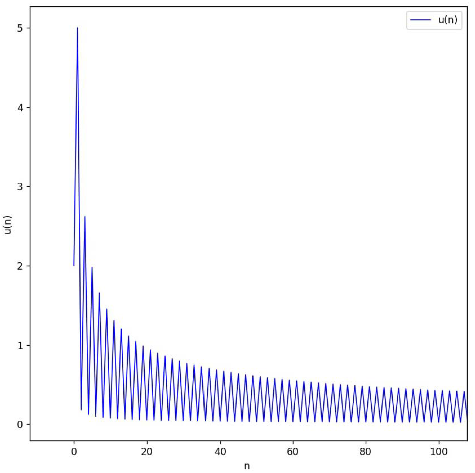
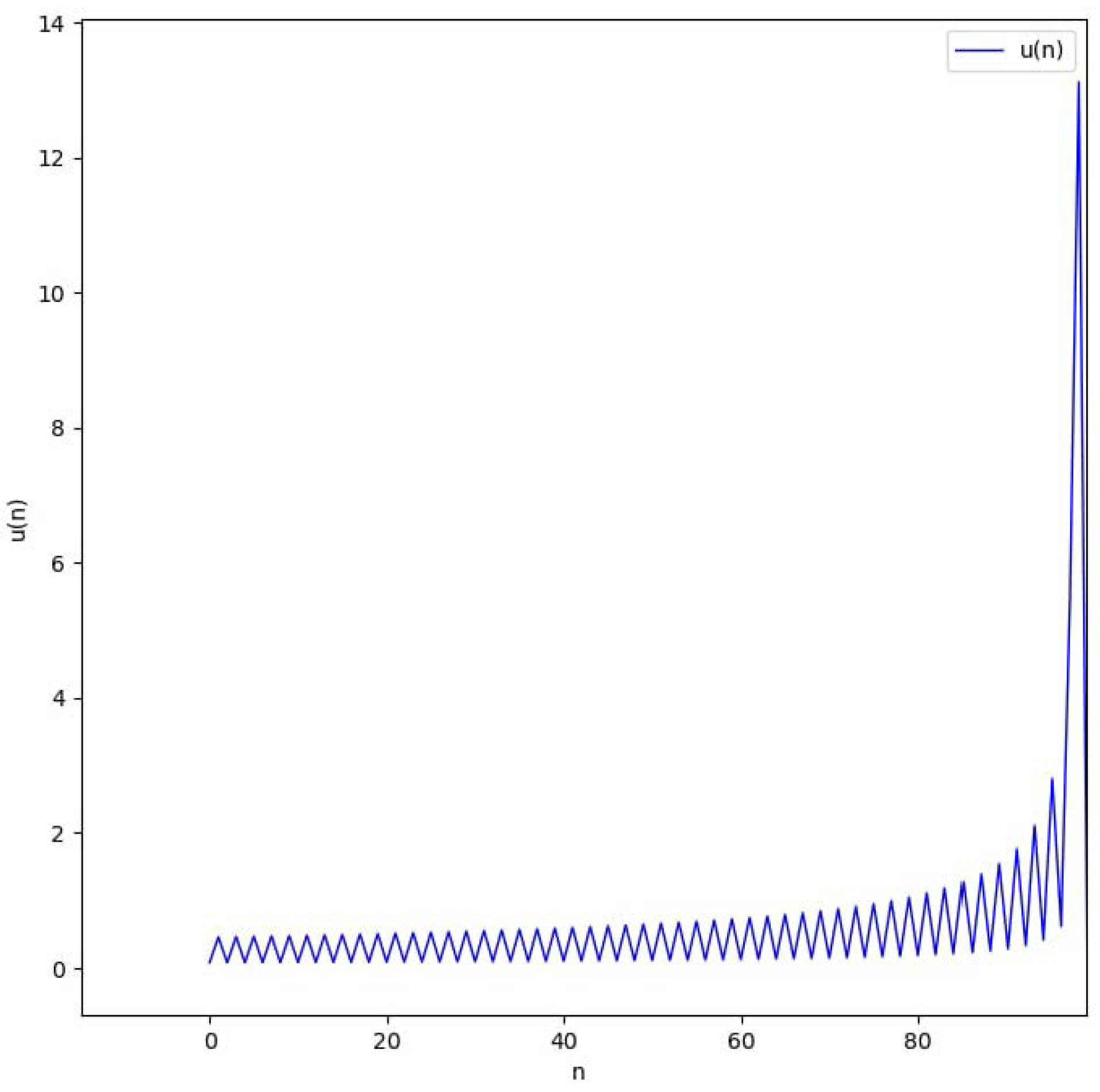
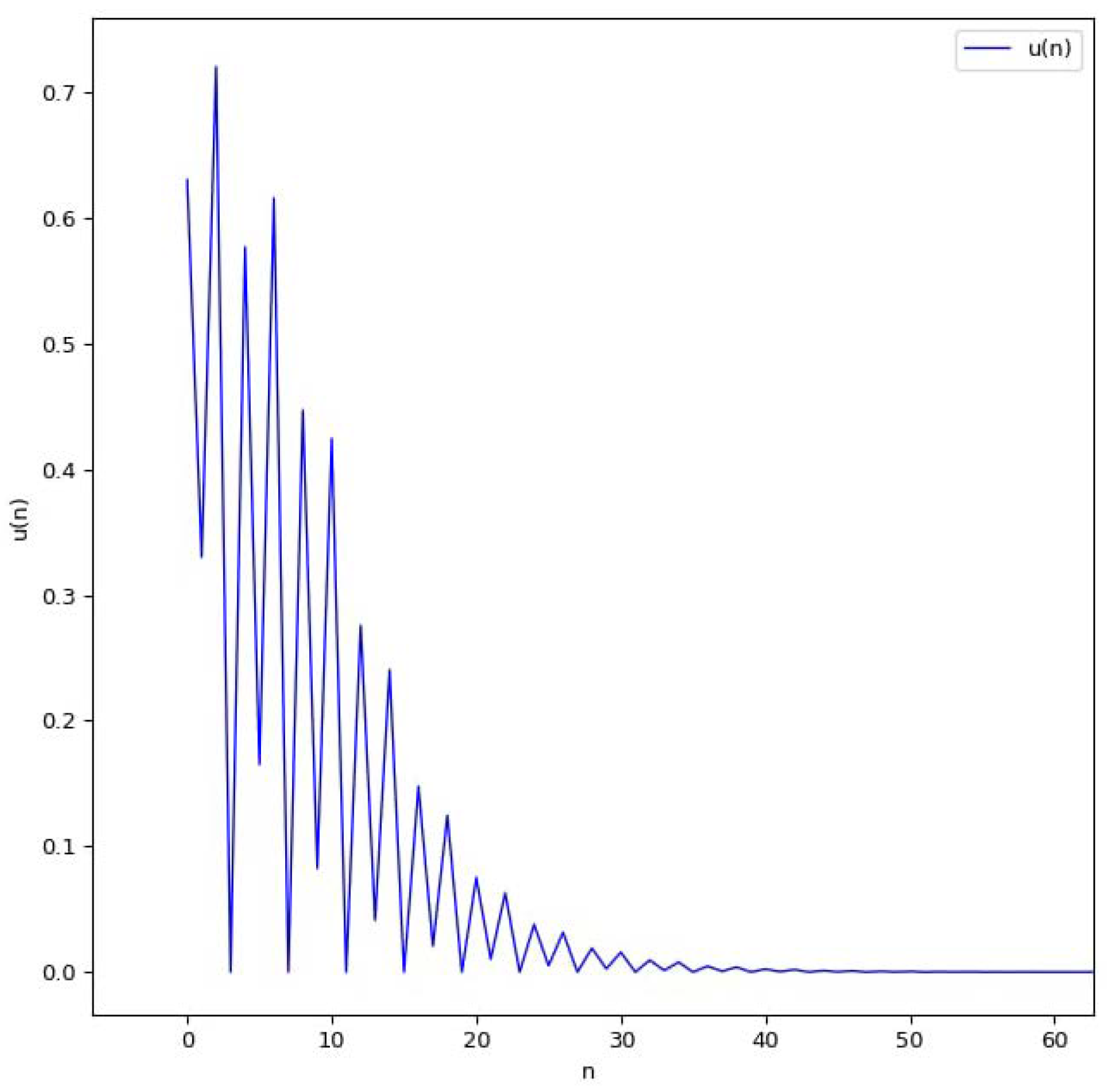
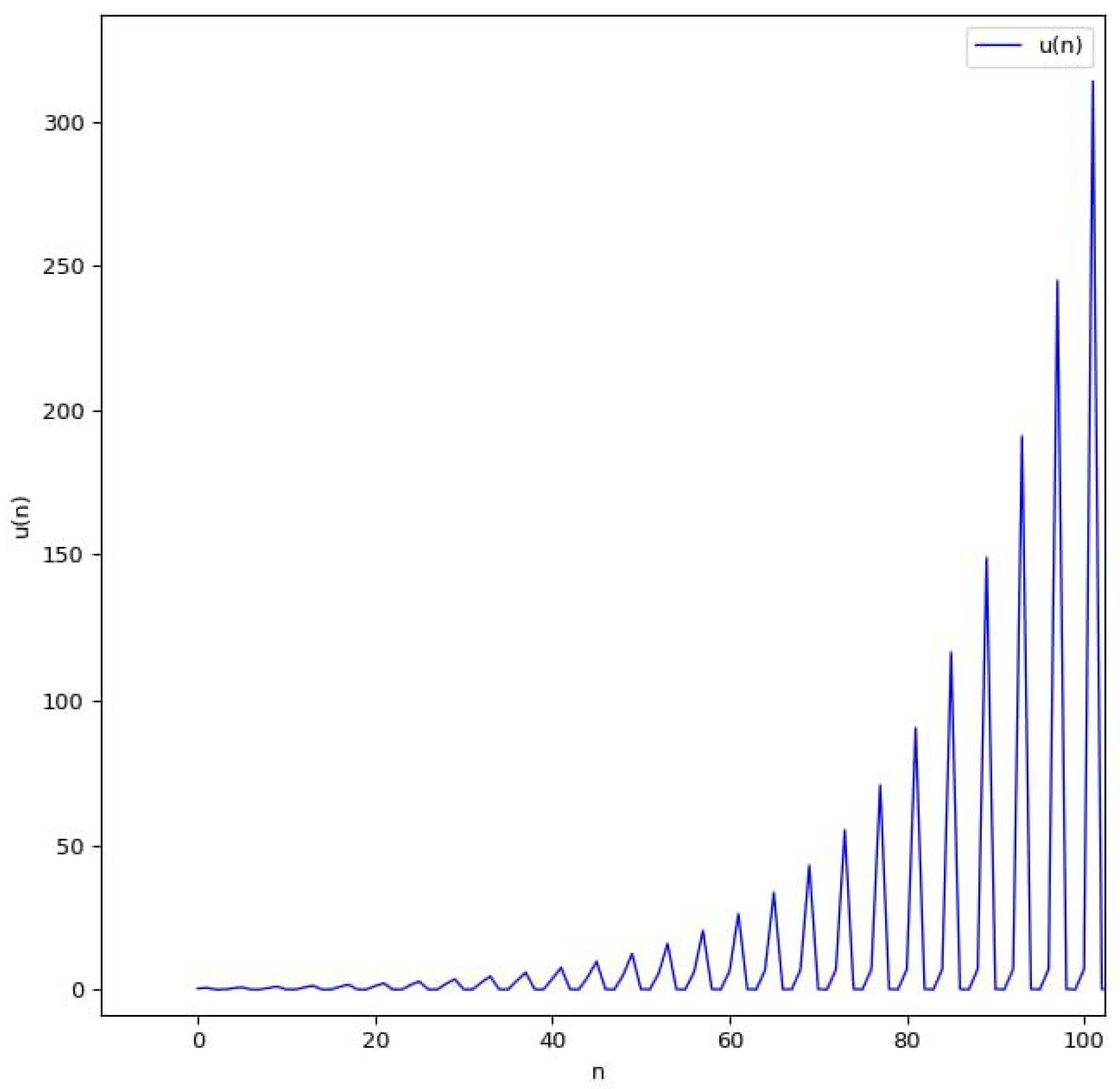
5. Numerical Examples

Below are some graphs that show the behavior of the solutions.

Example 1.

For the case with $A_n=1$, $B_n=B$ and $k=0$, where $u_{n+2}=\frac{u_n}{1+B{u}_n{u}_{n+1}}$, setting $A_n=1$, $B_n=B$, and $k=0$ in Equations (29) and (30) yields

$$\begin{array}{c}\hfill u_{2n}=u_0\prod _{k_0=0}^{n-1}\frac{1+2k_{0}B{u}_0{u}_1}{1+(2k_0+1)B{u}_0{u}_1}\end{array}$$

and

$$\begin{array}{c}\hfill u_{2n+1}=u_1\prod _{k_0=0}^{n-1}\frac{1+(2k_0+1)B{u}_0{u}_1}{1+(2k_0+2)B{u}_0{u}_1}.\end{array}$$

A sufficient condition for this solution to converge is given by $1+2k_{0}B{u}_0{u}_1<1+(2k_0+1)$$B{u}_0{u}_1$ and $1+(2k_0+1)B{u}_0{u}_1<1+(2k_0+2)B{u}_0{u}_1$ for $0\le k_0\le n-1$. This implies that $B{u}_0{u}_1>0$. It is then clear that if $B{u}_0{u}_1>0$, then the solution converges. On the other hand, a sufficient condition for this solution to diverge is given by $1+2k_{0}B{u}_0{u}_1>1+(2k_0+1)B{u}_0{u}_1$ or $1+(2k_0+1)B{u}_0{u}_1>1+(2k_0+2)B{u}_0{u}_1$ for $0\le k_0\le n-1$. This implies that $B{u}_0{u}_1<0$. It is then clear that if $B{u}_0{u}_1<0$, then the solution diverges.

Figure 1 shows the graph of $u_{n+2}=\frac{u_n}{1+u_n{u}_{n+1}}$ with $u_0=2$ and $u_1=5$. The solution converges as expected, since $B{u}_0{u}_1>0$.

Figure 2 shows the graph of $u_{n+2}=\frac{u_n}{1-0.28u_n{u}_{n+1}}$ with $u_0=0.08$ and $u_1=0.67$. The solution diverges as expected, since $B{u}_0{u}_1<0$.

Example 2.

In the case with $A_n=A\ne 1$, $B_n=B$, and $k=1$ such that $u_{n+4}=\frac{u_n}{A+B{u}_n{u}_{n+2}}$, setting $A_n=A$, $B_n=B$, and $k=1$ in Equations (29) and (30) yields

$$\begin{array}{cc}\hfill u_{4n}=& \frac{u_0}{A+B{u}_0{u}_2}{\displaystyle \prod _{k_0=1}^{n-1}}\frac{A^{2k_0}+B{u}_0{u}_2{\displaystyle \sum _{l=0}^{2k_0-1}}{A}^l}{A^{2k_0+1}+B{u}_0{u}_2{\displaystyle \sum _{l=0}^{2k_0}}{A}^l},\hfill \end{array}$$

(51)

$$\begin{array}{cc}\hfill u_{4n+1}=& \frac{u_1}{A+B{u}_1{u}_3}\prod _{k_0=1}^{n-1}\frac{A^{2k_0}+B{u}_1{u}_3{\displaystyle \sum _{l=0}^{2k_0-1}}{A}^l}{A^{2k_0+1}+B{u}_1{u}_3{\displaystyle \sum _{l=0}^{2k_0}}{A}^l},\hfill \end{array}$$

(52)

$$\begin{array}{cc}\hfill u_{4n+2}=& u_2\prod _{k_0=0}^{n-1}\frac{A^{2k_0+1}+B{u}_0{u}_2{\displaystyle \sum _{l=0}^{2k_0}}{A}^l}{A^{2k_0+2}+B{u}_0{u}_2{\displaystyle \sum _{l=0}^{2k_0+1}}{A}^l},\hfill \end{array}$$

(53)

$$\begin{array}{cc}\hfill u_{4n+3}=& u_3\prod _{k_0=0}^{n-1}\frac{A^{2k_0+1}+B{u}_1{u}_3{\displaystyle \sum _{l=0}^{2k_0}}{A}^l}{A^{2k_0+2}+B{u}_1{u}_3{\displaystyle \sum _{l=0}^{2k_0+1}}{A}^l}.\hfill \end{array}$$

(54)

Similarly, a sufficient condition for this solution to converge is for the numerators in Equations (51)–(54) to be less than their corresponding denominators. This implies that $B{u}_0{u}_2>1-A$ and $B{u}_1{u}_3>1-A$, where $A>0$. It is then clear that if $B{u}_0{u}_2>1-A$ and $B{u}_1{u}_3>1-A$, then the solution converges. On the other hand, a sufficient condition for this solution to diverge is for at least one of the numerators in Equations (51)–(54) to be greater than its corresponding denominator. This implies that $B{u}_0{u}_2<1-A$ or $B{u}_1{u}_3<1-A$, where $A>0$. It is then clear that if $B{u}_0{u}_2<1-A$ or $B{u}_1{u}_3<1-A$, then the solution diverges.

Figure 3 shows the graph of $u_{n+4}=\frac{u_n}{2-2u_n{u}_{n+2}}$ with $u_0=0.63,u_1=0.33,u_2=0.72$, and $u_3=0$. The solution converges as expected, since $B{u}_0{u}_2>1-A$ and $B{u}_1{u}_3>1-A$.

Figure 4 shows the graph of $u_{n+4}=\frac{u_n}{0.78+0.18u_n{u}_{n+2}}$ with $u_0=0.36,u_1=0.63,$$u_2=0.01$, and $u_3=0$. The solution diverges as expected, since $B{u}_0{u}_2<1-A$.

6. Conclusions

We obtained all the Lie point symmetries of the difference equation (Equation (12)). We used a symmetry-based method to derive its solutions. The solutions were given in ‘single’ form and then separated into $(2k+2)$ categories. We explained how the solutions of Equation (1) can be obtained using those of Equation (12) to show that the results in the recent literature can be obtained as special cases of our generalized solutions.

References

1. Cinar, C. On the positive solutions of the difference equation xn+1 = xn−1/(1 + xnxn−1). Appl. Math. Comput. 2004, 150, 21–24. [Google Scholar]
2. Cinar, C. On the difference equation xn+1 = xn−1/(−1 + xnxn−1). Appl. Math. Comput. 2004, 158, 813–816. [Google Scholar]
3. Cinar, C. On the positive solutions of the difference equation xn+1 = axn−1/(1 + bxnxn−1). Appl. Math. Comput. 2004, 156, 587–590. [Google Scholar]
4. Cinar, C. On the solutions of the difference equation xn+1 = xn−1/(−1 + axnxn−1). Appl. Math. Comput. 2004, 158, 793–797. [Google Scholar]
5. Cinar, C. On the positive solutions of the difference equation xn+1 = xn−1/(1 + axnxn−1). Appl. Math. Comput. 2004, 158, 809–812. [Google Scholar]
6. Aloqeili, M. Dynamics of a rational difference equation. Appl. Math. Comput. 2006, 176, 768–774. [Google Scholar] [CrossRef]
7. Elsayed, E.M. On the solution of some difference equation. Eur. J. Pure Appl. Math. 2011, 4, 287–303. [Google Scholar]
8. Elsayed, E.M. On the difference equation. Int. J. Contemp. Math. Sci. 2008, 3, 1657–1664. [Google Scholar]
9. Quispel, G.R.W.; Sahadevan, R. Lie symmetries and the integration of difference equations. Phys. Lett. A 1993, 184, 64–70. [Google Scholar] [CrossRef]
10. Hydon, P.E. Difference Equations by Differential Equation Methods; Cambridge University Press: Cambridge, UK, 2014. [Google Scholar]
11. Levi, D.; Vinet, L.; Winternitz, P. Lie group formalism for difference equations. J. Phys. A Math. Gen. 1997, 30, 633–649. [Google Scholar] [CrossRef]
12. Olver, P. Applications of Lie Groups to Differential Equations, 2nd ed.; Springer: New York, NY, USA, 1993. [Google Scholar]
13. Folly-Gbetoula, M.; Kara, A.H. Symmetries, conservation laws, and integrability of difference equations. Adv. Differ. Eq. 2014, 2014, 1–14. [Google Scholar] [CrossRef] [Green Version]
14. Hydon, P.E. Symmetries and first integrals of ordinary difference equations. Proc. R. Soc. Lond. A 2000, 456, 2835–2855. [Google Scholar] [CrossRef] [Green Version]
15. Folly-Gbetoula, M. Symmetry, reductions and exact solutions of the difference equation un+2 = aun/(1 + bunun+1). J. Diff. Eq. Appl. 2017, 23, 1017–1024. [Google Scholar] [CrossRef]
16. Yalcinkaya, I. On the global attractivity of positive solutions of a rational difference equation. Selcuk J. Appl. Math. 2008, 9, 3–8. [Google Scholar]
17. Karatas, R. On the solutions of the recursive sequence x n + 1 = a x n ( 2 k + 1 ) a + x n k x n ( 2 k + 1 ) . Fasc. Math. 2010, 45, 37–45. [Google Scholar]
18. Abdelrahman, M.A.E.; Chatzarakis, G.E.; Li, T.; Moaaz, O. On the difference equation xn+1 = axn−l + bxnk + f(xn−l,xnk). Adv. Differ. Eq. 2018, 431, 2018. [Google Scholar]
19. Joshi, N.; Vassiliou, P. The existence of Lie Symmetries for First-Order Analytic Discrete Dynamical Systems. J. Math. Anal. Appl. 1995, 195, 872–887. [Google Scholar] [CrossRef] [Green Version]
Figure 1. The graph of u n + 2 = u n 1 + u n u n + 1 .
Symmetry 14 01290 g001
Figure 2. The graph of u n + 2 = u n 1 0.28 u n u n + 1 .
Symmetry 14 01290 g002
Figure 3. The graph of u n + 4 = u n 2 2 u n u n + 2 .
Symmetry 14 01290 g003
Figure 4. The graph of u n + 4 = u n 0.78 + 0.18 u n u n + 2 .
Symmetry 14 01290 g004
Publisher’s Note: MDPI stays neutral with regard to jurisdictional claims in published maps and institutional affiliations.