Numerical Integration of Stiff Differential Systems Using Non-Fixed Step-Size Strategy

Abstract

Over the years, researches have shown that fixed (constant) step-size methods have been efficient in integrating a stiff differential system. It has however been observed that for some stiff differential systems, non-fixed (variable) step-size methods are required for efficiency and for accuracy to be attained. This is because such systems have solution components that decay rapidly and/or slowly than others over a given integration interval. In order to curb this challenge, there is a need to propose a method that can vary the step size within a defined integration interval. This challenge motivated the development of Non-Fixed Step-Size Algorithm (NFSSA) using the Lagrange interpolation polynomial as a basis function via integration at selected limits. The NFSSA is capable of integrating highly stiff differential systems in both small and large intervals and is also efficient in terms of economy of computer time. The validation of properties of the proposed algorithm which include order, consistence, zero-stability, convergence, and region of absolute stability were further carried out. The algorithm was then applied to solve some samples mildly and highly stiff differential systems and the results generated were compared with those of some existing methods in terms of the total number of steps taken, number of function evaluation, number of failure/rejected steps, maximum errors, absolute errors, approximate solutions and execution time. The results obtained clearly showed that the NFSSA performed better than the existing ones with which we compared our results including the inbuilt MATLAB stiff solver, ode 15s. The results were also computationally reliable over long intervals and accurate on the abscissae points which they step on.

1. Introduction

According to the authors in [1], a fixed step-size numerical integrator performs poorly if the solution (to the problem under consideration) varies rapidly at some points in the integration interval and slowly at other points of the integration interval. This major challenge motivated the conception of the idea of using non-fixed step-size strategy to propose an algorithm for the numerical integration of stiff differential systems of the form,

$$\begin{array}{l}y{}^{\prime }(x)=f\left(x,y(x)\right)\\ y(x_0)=y_0\end{array}\}$$

(1)

where $x\in [a,b]\subset \Re$, $f:\Re \times {\Re }^{2m}\to {\Re }^m$; $y(x),y_0\in {\Re }^m$, $m$ being the dimension of the differential system and the Jacobian $\left(\frac{\partial f}{\partial y}\right)$ with the negative real parts of its eigenvalues varies slowly. The functions $y(x)$ and $f\left(x,y(x)\right)$ are assumed to satisfy the existence and uniqueness theorem stated in Theorem 1.

Theorem 1.

[2] “Let

$$y^{(n)}(x)=f\left(x,y(x),y{}^{\prime }(x),\dots ,y^{(n-1)}(x)\right),y^{(k)}(x_0)=c_k$$

(2)

where $k=0,1,\dots ,(n-1)$ and let $\Re$ be the region defined by the inequalities $x_0\le x\le x_0+a$, $\left|s_j-c_j\right|\le b$, $j=0,1,\dots ,(n-1)$, $a>0$ and $b>0$. Suppose the function $f\left(x,s_0,s_1,\dots ,s_{n-1}\right)$ is defined in $\Re$ and in addition,

i 

$f$is non-negative and non-decreasing in each$x,s_0,s_1,\dots ,s_{n-1}$in$\Re$,

ii 

$f\left(x,c_0,c_1,\dots ,c_{n-1}\right)>0$for$x_0\le x\le x_0+a$, and

iii 

$c_k\ge 0,k=0,1,\dots ,n-1$.

Then the initial value problem (2) has a unique solution in $\Re$”.

For the Proof of Theorem 1, see [2].

Stiff differential systems of the Form (1) are special problems that arise most often in different areas of science and engineering. These systems find applications in chemical kinetics, mechanics, lasers, control systems, molecular dynamics, biological models and electronic circuits [3,4]. Stiffness does not have a unique definition; some definitions of stiffness are found in [5,6,7,8]. In study [5], a chemist was the first to identify stiff systems. The author stated that implicit methods perform better than explicit methods on stiff differential systems. In fact, the explicit methods do not work on some stiff systems. Suffice to say that the proposed NFSSA will be implicit in nature. It is also hoped that the proposed NFSSA will efficiently integrate highly stiff differential systems of the Form (1) over large intervals. One of the ways to integrate a stiff differential system efficiently and accurately is by developing the implicit block method. Block methods have been known to have the capability of generating multiple solutions simultaneously in a single integration. Moreover, block methods require a fewer number of function evaluations per step and also reduce computational time. The proposed NFSSA (which is a modification of the block method) will be implemented in a hybrid mode, with the insertion of two off-grid points at selected points.

Different methods have been proposed by authors for the numerical integration of mildly stiff differential systems of the Form (1). These methods include direct methods, variation methods, nonstandard finite difference methods, Adomian decomposition methods, linear multistep methods, Second Derivative Methods (SDMs), Block Backward Differentiation Formulas (BBDFs), among others. These methods are mostly derived using the fixed (constant) step-size strategy [9,10,11,12,13,14,15,16]. Highly stiff large systems were also integrated numerically using different methods [17,18,19,20,21,22]. On the other hand, the authors in [23,24,25,26,27,28,29,30,31,32,33,34,35,36,37,38] formulated different methods using the non-fixed (variable) step-size strategy for the solution of stiff differential systems. These methods have shown to be more efficient and accurate than the fixed step-size methods. For instance, study [1] proposed a variable step-size block method for the solution of stiff systems. The A-stable method which is of order 6 is in the form of Simpson’s type block variable step-size method. The method simultaneously generated results of the stiff system at defined grid points. The authors in [33] further formulated a variable step hybrid block method (via the block backward differentiation approach) for solving stiff chemical kinetics problems. The authors used the step-size ratios $r=1$, $r=2$ and $r=10/19$. They further analysed the properties of the method. The method formulated was found to be computationally reliable on chemical kinetics problems.

The literature reviewed above motivated this study, which has to do with the development of an NFSSA for the numerical integration of stiff differential systems of the Form (1). It is hoped that the new algorithm will be computationally reliable over long intervals and accurate on the abscissae points they step on.

This paper is organized as follows: Section 2 clearly explains the derivation of the NFSSA. In Section 3, the properties of the newly derived NFSSA are validated. The pseudocode and step-size selection for the NFSSA are presented in Section 4 while numerical examples are given in Section 5. Section 6 highlights the results and discussion. Finally, the conclusions are drawn in Section 7.

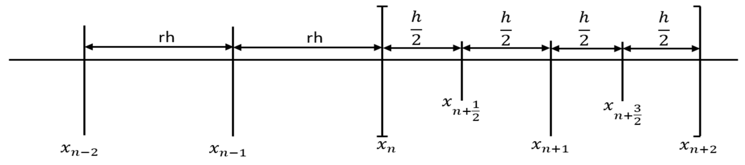
2. Derivation of the NFSSA

In this section, the derivation of the proposed NFSSA is discussed in detail. For clarity, Figure 1 shows the points $x_{n-2}$, $x_{n-1}$ and $x_n$ (each having the step-size $rh$) as starting values and the off-step points $x_{n+1/2}$ and $x_{n+3/2}$ (each having half step-size $h/2$). Note that $r$ is the step-size ratio. The predictor formulae will involve the set of points $\left(x_{n-2},x_{n-1},x_n\right)$ while the corrector formulae will involve the set of points $\left(x_{n-2},x_{n-1},x_n,x_{n+1/2},x_{n+1},x_{n+3/2},x_{n+2}\right)$. In order to optimize the total number of steps, ensure zero-stability and minimize the number of formulae stored in the code, the step-size ratio $r$ is maintained $(r=1)$, halved $(r=2)$ or doubled $(r=1/2)$. This approach is sometimes called the Milne device [39]. This strategy was first suggested by [40,41].

Consider the $k$-step Linear Multistep Method (LMM) defined as,

$${\displaystyle \sum _{j=1}^k{\alpha }_j{y}_{n+j}=h^{\mu }{\displaystyle \sum _{j=1}^k{\beta }_j{f}_{n+j}}}$$

(3)

where ${\alpha }_j’s$ and ${\beta }_j’s$ are real constant coefficients and $\mu$ is the order of the differential equation. Equation (3) is explicit if ${\beta }_k=0$ and implicit if ${\beta }_k\ne 0$. The proposed NFSSA shall consist of LMMs (at the grid points $x_{n+1/2}$, $x_{n+1}$, $x_{n+3/2}$ and $x_{n+2}$) which will be implemented in a block form. To derive the NFSSA at the points $x_{n+r},r=\frac{1}{2},1,\frac{3}{2}$ and $2$, Equation (1) is integrated in the interval $(x_n,x_{n+r})$,

$${\displaystyle \underset{x_n}{\overset{x_{n+r}}{\int }}y{}^{\prime }(x)dx={\displaystyle \underset{x_n}{\overset{x_{n+r}}{\int }}f\left(x,y(x)\right)dx}}$$

(4)

The Lagrange polynomial $P_q(x)$ is used in approximating the function $f\left(x,y(x)\right)$ in Equation (1). That is,

$$P_q(x)={\displaystyle \sum _{j=0}^k{L}_{q,j}(x)f(x_{n+2-j})}$$

(5)

where

$$L_{q,j}(x)={\displaystyle \prod _{\begin{array}{l}i=0\\ i\ne j\end{array}}^{k-1}\frac{x-x_{n+2-i}}{x_{n+2-j}-x_{n+2-i}}},j=0,\frac{1}{2},1,2,\dots ,k$$

The corrector formulae for $y_{n+1/2}$, $y_{n+1}$, $y_{n+3/2}$ and $y_{n+2}$ are obtained using the Lagrange interpolation polynomial,

$$\begin{array}{l}{P}_2(x)=\left[\frac{(x-x_{n-2})(x-x_{n-1})(x-x_n)(x-x_{n+1/2})(x-x_{n+1})(x-x_{n+3/2})}{(x_{n+2}-x_{n-2})(x_{n+2}-x_{n-1})(x_{n+2}-x_n)(x_n-x_{n+1/2})(x_{n+2}-x_{n+1})(x_{n+2}-x_{n+3/2})}\right]f(x_{n+2})\\ \hspace{1em} +\left[\frac{(x-x_{n-2})(x-x_{n-1})(x-x_n)(x-x_{n+1/2})(x-x_{n+1})(x-x_{n+2})}{(x_{n+3/2}-x_{n-2})(x_{n+3/2}-x_{n-1})(x_{n+3/2}-x_n)(x_{n+3/2}-x_{n+1/2})(x_{n+3/2}-x_{n+1})(x_{n+3/2}-x_{n+2})}\right]f(x_{n+3/2})\\ \hspace{1em} +\left[\frac{(x-x_{n-2})(x-x_{n-1})(x-x_n)(x-x_{n+1/2})(x-x_{n+3/2})(x-x_{n+2})}{(x_{n+1}-x_{n-2})(x_{n+1}-x_{n-1})(x_{n+1}-x_n)(x_{n+1}-x_{n+1/2})(x_{n+1}-x_{n+3/2})(x_{n+1}-x_{n+2})}\right]f(x_{n+1})\\ \hspace{1em} +\left[\frac{(x-x_{n-2})(x-x_{n-1})(x-x_n)(x-x_{n+1})(x-x_{n+3/2})(x-x_{n+2})}{(x_{n+1/2}-x_{n-2})(x_{n+1/2}-x_{n-1})(x_{n+1/2}-x_n)(x_{n+1/2}-x_{n+1})(x_{n+1/2}-x_{n+3/2})(x_{n+1/2}-x_{n+2})}\right]f(x_{n+1/2})\\ \hspace{1em} +\left[\frac{(x-x_{n-2})(x-x_{n-1})(x-x_{n+1/2})(x-x_{n+1})(x-x_{n+3/2})(x-x_{n+2})}{(x_n-x_{n-2})(x_n-x_{n-1})(x_n-x_{n+1/2})(x_n-x_{n+1})(x_n-x_{n+3/2})(x_n-x_{n+2})}\right]f(x_n)\\ \hspace{1em} +\left[\frac{(x-x_{n-2})(x-x_n)(x-x_{n+1/2})(x-x_{n+1})(x-x_{n+3/2})(x-x_{n+2})}{(x_{n-1}-x_{n-2})(x_{n-1}-x_n)(x_{n-1}-x_{n+1/2})(x_{n-1}-x_{n+1})(x_{n-1}-x_{n+3/2})(x_{n-1}-x_{n+2})}\right]f(x_{n-1})\\ \hspace{1em} +\left[\frac{(x-x_{n-1})(x-x_n)(x-x_{n+1/2})(x-x_{n+1})(x-x_{n+3/2})(x-x_{n+2})}{(x_{n-2}-x_{n-1})(x_{n-2}-x_n)(x_{n-2}-x_{n+1/2})(x_{n-2}-x_{n+1})(x_{n-2}-x_{n+3/2})(x_{n-2}-x_{n+2})}\right]f(x_{n-2})\end{array}$$

(6)

at the interpolation points $(x_{n-2},y_{n-2})$, $(x_{n-1},y_{n-1})$, $(x_n,y_n)$,$\left(x_{n+1/2},y_{n+1/2}\right)$, $(x_{n+1},y_{n+1})$,$\left(x_{n+3/2},y_{n+3/2}\right)$ and $(x_{n+2},y_{n+2})$.

The corrector NFSSA at $y_{n+1/2}$, $y_{n+1}$, $y_{n+3/2}$ and $y_{n+2}$ are derived by integrating Equation (1) with respect to $s$, $s=(x-x_{n+2})/h$, replacing $dx$ by $hds$ and taking the limits of integration at (−2, −3/2), (−2, −1), (−2, −1/2) and (−2, 0), respectively. This gives,

$$\begin{array}{l}{y}_{n+\frac{1}{2}}=y_n+\left[\left(\frac{h}{5376r^2}\right)\left(\frac{189r+41}{32r^4+80r^3+70r^2+25r+3}\right)\right]f_{n-2}-\left[\left(\frac{h}{1344r^2}\right)\left(\frac{378r+41}{4r^4+20r^3+35r^2+25r+6}\right)\right]f_{n-1}\\ +\left[\left(\frac{h}{\mathrm{80,640}{r}^2}\right)\left(\mathrm{14,056}{r}^2+2835r+205\right)\right]f_n+\left[\left(\frac{h}{2520}\right)\left(\frac{9044r^2+3948r+453}{8r^2+6r+1}\right)\right]f_{n+\frac{1}{2}}\\ -\left[\left(\frac{h}{6720}\right)\left(\frac{2464r^2+861r+82}{2r^2+3r+1}\right)\right]f_{n+1}+\left[\left(\frac{h}{2520}\right)\left(\frac{1484r^2+504r+47}{8r^2+18r+9}\right)\right]f_{n+\frac{3}{2}}-\left[\left(\frac{h}{\mathrm{80,640}}\right)\left(\frac{1064r^2+357r+33}{r^2+3r+2}\right)\right]f_{n+2}\end{array}$$

(7)

$$\begin{array}{l}{y}_{n+1}=y_n+\left[\left(\frac{h}{336r^2}\right)\left(\frac{7r-1}{32r^4+80r^3+70r^2+25r+3}\right)\right]f_{n-2}-\left[\left(\frac{h}{84r^2}\right)\left(\frac{14r-1}{4r^4+20r^3+35r^2+25r+6}\right)\right]f_{n-1}\\ +\left[\left(\frac{h}{5040r^2}\right)\left(812r^2+105r-5\right)\right]f_n+\left[\left(\frac{4h}{315}\right)\left(\frac{434r^2+273r+48}{8r^2+6r+1}\right)\right]f_{n+\frac{1}{2}}\\ +\left[\left(\frac{h}{420}\right)\left(\frac{112r^2+273r+86}{2r^2+3r+1}\right)\right]f_{n+1}-\left[\left(\frac{4h}{315}\right)\left(\frac{-14r^2+21r+8}{8r^2+18r+9}\right)\right]f_{n+\frac{3}{2}}+\left[\left(\frac{h}{5040}\right)\left(\frac{-28r^2+21r+9}{r^2+3r+2}\right)\right]f_{n+2}\end{array}$$

(8)

$$\begin{array}{l}{y}_{n+\frac{3}{2}}=y_n+\left[\left(\frac{9h}{1792r^2}\right)\left(\frac{7r+3}{32r^4+80r^3+70r^2+25r+3}\right)\right]f_{n-2}-\left[\left(\frac{9h}{448r^2}\right)\left(\frac{14r+3}{4r^4+20r^3+35r^2+25r+6}\right)\right]f_{n-1}\\ +\left[\left(\frac{9h}{8960r^2}\right)\left(168r^2+35r+5\right)\right]f_n+\left[\left(\frac{3h}{280}\right)\left(\frac{476r^2+252r+27}{8r^2+6r+1}\right)\right]f_{n+\frac{1}{2}}\\ +\left[\left(\frac{9h}{2240}\right)\left(\frac{224r^2+441r+162}{2r^2+3r+1}\right)\right]f_{n+1}+\left[\left(\frac{3h}{280}\right)\left(\frac{196r^2+336r+153}{8r^2+18r+9}\right)\right]f_{n+\frac{3}{2}}-\left[\left(\frac{3h}{8960}\right)\left(\frac{56r^2+63r+27}{r^2+3r+2}\right)\right]f_{n+2}\end{array}$$

(9)

$$\begin{array}{l}{y}_{n+2}=y_n+\left[\left(\frac{-h}{21r^2}\right)\left(\frac{1}{32r^4+80r^3+70r^2+25r+3}\right)\right]f_{n-2}+\left[\left(\frac{4h}{21r^2}\right)\left(\frac{1}{4r^4+20r^3+35r^2+25r+6}\right)\right]f_{n-1}\\ +\left[\left(\frac{h}{315r^2}\right)\left(49r^2-5\right)\right]f_n+\left[\left(\frac{64h}{315}\right)\left(\frac{28r^2+21r+6}{8r^2+6r+1}\right)\right]f_{n+\frac{1}{2}}\\ +\left[\left(\frac{4h}{105}\right)\left(\frac{14r^2+21r+2}{2r^2+3r+1}\right)\right]f_{n+1}+\left[\left(\frac{64h}{315}\right)\left(\frac{28r^2+63r+34}{8r^2+18r+9}\right)\right]f_{n+\frac{3}{2}}+\left[\left(\frac{h}{315}\right)\left(\frac{49r^2+147r+93}{r^2+3r+2}\right)\right]f_{n+2}\end{array}$$

(10)

Substituting $r=1$, $r=2$ and $r=1/2$ into Equations (7)–(10) gives the NFSSA displayed in

Table 1. Formulae of the NFSSA.

Step-Size	Formulae
Ratio
$r=1$	$y_{n+\frac{1}{2}}=y_n+h\left(\frac{23}{\mathrm{112,896}}{f}_{n-2}-\frac{419}{\mathrm{120,960}}{f}_{n-1}+\frac{2137}{\mathrm{10,080}}{f}_n+\frac{2689}{7560}{f}_{n+\frac{1}{2}}-\frac{3407}{\mathrm{40,320}}{f}_{n+1}+\frac{407}{\mathrm{17,640}}{f}_{n+\frac{3}{2}}-\frac{727}{\mathrm{241,920}}{f}_{n+2}\right)$
	$y_{n+1}=y_n+h\left(\frac{1}{\mathrm{11,760}}{f}_{n-2}-\frac{13}{7560}{f}_{n-1}+\frac{19}{105}{f}_n+\frac{604}{945}{f}_{n+\frac{1}{2}}+\frac{157}{840}{f}_{n+1}-\frac{4}{735}{f}_{n+\frac{3}{2}}+\frac{1}{\mathrm{15,120}}{f}_{n+2}\right)$
	$y_{n+\frac{3}{2}}=y_n+h\left(\frac{3}{\mathrm{12,544}}{f}_{n-2}-\frac{17}{4480}{f}_{n-1}+\frac{117}{560}{f}_n+\frac{151}{280}{f}_{n+\frac{1}{2}}+\frac{2481}{4480}{f}_{n+1}+\frac{411}{1960}{f}_{n+\frac{3}{2}}-\frac{73}{8960}{f}_{n+2}\right)$
	$y_{n+2}=y_n+h\left(-\frac{1}{4410}{f}_{n-2}+\frac{2}{945}{f}_{n-1}+\frac{44}{315}{f}_n+\frac{704}{945}{f}_{n+\frac{1}{2}}+\frac{74}{315}{f}_{n+1}+\frac{320}{441}{f}_{n+\frac{3}{2}}+\frac{289}{1890}{f}_{n+2}\right)$
$r=2$	$y_{n+\frac{1}{2}}=y_n+h\left(\frac{419}{\mathrm{31,933,440}}{f}_{n-2}-\frac{797}{\mathrm{2,257,920}}{f}_{n-1}+\frac{\mathrm{62,099}}{\mathrm{322,560}}{f}_n+\frac{1781}{4536}{f}_{n+\frac{1}{2}}-\frac{583}{5040}{f}_{n+1}+\frac{6991}{\mathrm{194,040}}{f}_{n+\frac{3}{2}}-\frac{5003}{\mathrm{967,680}}{f}_{n+2}\right)$
	$y_{n+1}=y_n+h\left(\frac{13}{\mathrm{1,995,840}}{f}_{n-2}-\frac{3}{\mathrm{15,680}}{f}_{n-1}+\frac{1151}{6720}{f}_n+\frac{1864}{2835}{f}_{n+\frac{1}{2}}+\frac{6}{35}{f}_{n+1}+\frac{8}{8085}{f}_{n+\frac{3}{2}}-\frac{61}{\mathrm{60,480}}{f}_{n+2}\right)$
	$y_{n+\frac{3}{2}}=y_n+h\left(\frac{17}{\mathrm{1,182,720}}{f}_{n-2}-\frac{93}{\mathrm{250,880}}{f}_{n-1}+\frac{6723}{\mathrm{35,840}}{f}_n+\frac{487}{840}{f}_{n+\frac{1}{2}}+\frac{291}{560}{f}_{n+1}+\frac{4827}{\mathrm{21,560}}{f}_{n+\frac{3}{2}}-\frac{377}{\mathrm{35,840}}{f}_{n+2}\right)$
	$y_{n+2}=y_n+h\left(-\frac{1}{\mathrm{124,740}}{f}_{n-2}+\frac{1}{8820}{f}_{n-1}+\frac{191}{1260}{f}_n+\frac{2048}{2835}{f}_{n+\frac{1}{2}}+\frac{16}{63}{f}_{n+1}+\frac{\mathrm{17,408}}{\mathrm{24,255}}{f}_{n+\frac{3}{2}}+\frac{583}{3780}{f}_{n+2}\right)$
$r=\frac{1}{2}$	$y_{n+\frac{1}{2}}=y_n+h\left(\frac{271}{\mathrm{120,960}}{f}_{n-2}-\frac{23}{1008}{f}_{n-1}+\frac{\mathrm{10,273}}{\mathrm{40,320}}{f}_n+\frac{293}{945}{f}_{n+\frac{1}{2}}-\frac{2257}{\mathrm{40,320}}{f}_{n+1}+\frac{67}{5040}{f}_{n+\frac{3}{2}}-\frac{191}{\mathrm{120,960}}{f}_{n+2}\right)$
	$y_{n+1}=y_n+h\left(\frac{1}{1512}{f}_{n-2}-\frac{1}{105}{f}_{n-1}+\frac{167}{840}{f}_n+\frac{586}{945}{f}_{n+\frac{1}{2}}+\frac{167}{840}{f}_{n+1}-\frac{1}{105}{f}_{n+\frac{3}{2}}+\frac{1}{1512}{f}_{n+2}\right)$
	$y_{n+\frac{3}{2}}=y_n+h\left(\frac{13}{4480}{f}_{n-2}-\frac{3}{112}{f}_{n-1}+\frac{1161}{4480}{f}_n+\frac{17}{35}{f}_{n+\frac{1}{2}}+\frac{2631}{4480}{f}_{n+1}+\frac{111}{560}{f}_{n+\frac{3}{2}}-\frac{29}{4480}{f}_{n+2}\right)$
	$y_{n+2}=y_n+h\left(-\frac{4}{945}{f}_{n-2}+\frac{8}{315}{f}_{n-1}+\frac{29}{315}{f}_n+\frac{752}{945}{f}_{n+\frac{1}{2}}+\frac{64}{315}{f}_{n+1}+\frac{323}{315}{f}_{n+\frac{3}{2}}+\frac{143}{945}{f}_{n+2}\right)$

.

The newly derived NFSSA shall be implemented in predictor-corrector mode. The predictor formulae which were derived using the same procedure with that of the corrector formulae are thus given as,

$$y_{n+\frac{1}{2}}=y_n+\left[\left(\frac{h}{48r^2}\right)\left(3r+1\right)\right]f_{n-2}-\left[\left(\frac{h}{24r^2}\right)\left(6r+1\right)\right]f_{n-1}+\left[\left(\frac{h}{48r^2}\right)\left(24r^2+9r+1\right)\right]f_n$$

(11)

$$y_{n+1}=y_n+\left[\left(\frac{h}{12r^2}\right)\left(3r+2\right)\right]f_{n-2}-\left[\left(\frac{h}{3r^2}\right)\left(3r+1\right)\right]f_{n-1}+\left[\left(\frac{h}{12r^2}\right)\left(12r^2+9r+2\right)\right]f_n$$

(12)

$$y_{n+\frac{3}{2}}=y_n+\left[\left(\frac{3h}{16r^2}\right)\left(8r^2+9r+3\right)\right]f_{n-2}-\left[\left(\frac{9h}{8r^2}\right)\left(2r+1\right)\right]f_{n-1}+\left[\left(\frac{9h}{16r^2}\right)\left(r+1\right)\right]f_n$$

(13)

$$y_{n+2}=y_n+\left[\left(\frac{h}{3r^2}\right)\left(3r+4\right)\right]f_{n-2}-\left[\left(\frac{4h}{3r^2}\right)\left(3r+2\right)\right]f_{n-1}+\left[\left(\frac{h}{3r^2}\right)\left(6r^2+9r+4\right)\right]f_n$$

(14)

Substituting the step-size ratios $r=1$, $r=2$ and $r=1/2$ into Equations (11)–(14) gives the explicit formulae of the predictor NFSSA with the interpolation points $\left(x_{n-2},f_{n-2}\right)$, $\left(x_{n-1},f_{n-1}\right)$ and $\left(x_n,f_n\right)$ as presented in

Table 2. Predictor formulae of the NFSSA.

Step-Size Ratio	Predictor Formulae
$r=1$	$y_{n+\frac{1}{2}}^p=y_n+\frac{h}{12}\left(f_{n-2}-\frac{7}{2}{f}_{n-1}+\frac{17}{2}{f}_n\right)$
	$y_{n+1}^p=y_n+\frac{h}{3}\left(\frac{5}{4}{f}_{n-2}-4f_{n-1}+\frac{23}{4}{f}_n\right)$
	$y_{n+\frac{3}{2}}^p=y_n+\frac{h}{4}\left(\frac{9}{2}{f}_{n-2}-\frac{27}{2}{f}_{n-1}+15f_n\right)$
	$y_{n+2}^p=y_n+\frac{h}{3}\left(7f_{n-2}-20f_{n-1}+19f_n\right)$
$r=2$	$y_{n+\frac{1}{2}}^p=y_n+\frac{h}{96}\left(\frac{7}{2}{f}_{n-2}-13f_{n-1}+\frac{115}{2}{f}_n\right)$
	$y_{n+1}^p=y_n+\frac{h}{6}\left(f_{n-2}-\frac{7}{2}{f}_{n-1}+\frac{17}{2}{f}_n\right)$
	$y_{n+\frac{3}{2}}^p=y_n+\frac{h}{32}\left(\frac{27}{2}{f}_{n-2}-45f_{n-1}+\frac{159}{2}{f}_n\right)$
	$y_{n+2}^p=y_n+\frac{h}{3}\left(\frac{5}{2}{f}_{n-2}-8f_{n-1}+\frac{23}{2}{f}_n\right)$
$r=\frac{1}{2}$	$y_{n+\frac{1}{2}}^p=y_n+\frac{h}{3}\left(\frac{5}{8}{f}_{n-2}-2f_{n-1}+\frac{23}{8}{f}_n\right)$
	$y_{n+1}^p=y_n+\frac{h}{3}\left(\frac{7}{2}{f}_{n-2}-10f_{n-1}+\frac{19}{2}{f}_n\right)$
	$y_{n+\frac{3}{2}}^p=y_n+\frac{h}{8}\left(27f_{n-2}-72f_{n-1}+57f_n\right)$
	$y_{n+2}^p=y_n+\frac{h}{3}\left(22f_{n-2}-56f_{n-1}+40f_n\right)$

.

3. Validation of Properties of the NFSSA

The properties of the proposed NFSSA shall be validated in this section.

3.1. Order and Error Constant

Definition 1.

[42] “The LMM (3) and its associated difference operator $L$ defined by

$$L\left\{y(x);h\right\}={\displaystyle \sum _{j=0}^k\left[{\alpha }_{j}y(x+jh)-h{\beta }_{j}y{}^{\prime }(x+jh)\right]}$$

(15)

are said to be of order $p$ if $c_0=c_1=c_2=\dots =c_p=0,c_{p+1}\ne 0$”.

The term $c_{p+1}\ne 0$ is the error constant of the method. The general form for the constant $c_p$ is defined as,

$$\begin{array}{l}{c}_0={\displaystyle \sum _{j=0}^k{\alpha }_j}\\ c_1={\displaystyle \sum _{j=0}^k\left(j{\alpha }_j-{\beta }_j\right)}\\ .\\ .\\ .\\ c_p={\displaystyle \sum _{j=0}^k\left[\frac{1}{p!}{j}^p{\alpha }_j-\frac{1}{(p-1)!}{j}^{p-1}{\beta }_j\right]},p=2,3,\dots ,q+1\end{array}\}$$

(16)

Equation (16) is applied to the NFSSA at the step ratio $r=1$. This produces

$$c_0=c_1=c_2=c_3=c_4=c_5=c_6=c_7=\left[\begin{array}{l}0\\ 0\\ 0\\ 0\end{array}\right]$$

(17)

Thus, the NFSSA is of the seventh order with the error constant,

$$c_8=\left[\begin{array}{l}1.8901\times {10}^{-5}\\ 5.3146\times {10}^{-5}\\ 2.6282\times {10}^{-5}\\ -4.7241\times {10}^{-5}\end{array}\right]$$

(18)

The same approach applies to the NFSSA at $r=2$ and $r=1/2$.

3.2. Zero-Stability

Definition 2.

[43] “If no root of the characteristic polynomial has a modulus greater than one and every root with modulus one is simple, then such a method is called zero-stable”.

The zero-stability of a method controls the propagation of errors as the integration progresses. It is determined by using the linear scalar test equation given by [40] as,

$$y{}^{\prime }(x)=\lambda y(x)$$

(19)

where $\mathrm{Re}(\lambda )<0,\lambda$ being a complex constant. Substituting Equation (19) into the NFSSA at $r=1$ gives,

$$\begin{array}{l}{y}_{n+\frac{1}{2}}=y_n+h\left(\frac{23}{\mathrm{112,896}}\lambda y_{n-2}-\frac{419}{\mathrm{120,960}}\lambda y_{n-1}+\frac{2137}{\mathrm{10,080}}\lambda y_n+\frac{2689}{7560}\lambda y_{n+\frac{1}{2}}-\frac{3407}{\mathrm{40,320}}\lambda y_{n+1}+\frac{407}{\mathrm{17,640}}\lambda y_{n+\frac{3}{2}}-\frac{727}{\mathrm{241,920}}\lambda y_{n+2}\right)\\ y_{n+1}=y_n+h\left(\frac{1}{\mathrm{11,760}}\lambda y_{n-2}-\frac{13}{7560}\lambda y_{n-1}+\frac{19}{105}\lambda y_n+\frac{604}{945}\lambda y_{n+\frac{1}{2}}-\frac{157}{840}\lambda y_{n+1}-\frac{4}{735}\lambda y_{n+\frac{3}{2}}+\frac{1}{\mathrm{15,120}}\lambda y_{n+2}\right)\\ y_{n+\frac{3}{2}}=y_n+h\left(\frac{3}{\mathrm{12,544}}\lambda y_{n-2}-\frac{17}{4480}\lambda y_{n-1}+\frac{117}{560}\lambda y_n+\frac{151}{280}\lambda y_{n+\frac{1}{2}}+\frac{2481}{4480}\lambda y_{n+1}+\frac{411}{1960}\lambda y_{n+\frac{3}{2}}-\frac{73}{8960}\lambda y_{n+2}\right)\\ y_{n+2}=y_n+h\left(-\frac{1}{4410}\lambda y_{n-2}+\frac{2}{945}\lambda y_{n-1}+\frac{44}{315}\lambda y_n+\frac{704}{945}\lambda y_{n+\frac{1}{2}}+\frac{74}{315}\lambda y_{n+1}+\frac{320}{441}\lambda y_{n+\frac{3}{2}}+\frac{289}{1890}\lambda y_{n+2}\right)\end{array}\}$$

(20)

In matrix form, we rewrite Equation (20) as,

$$\begin{array}{c}\left[\begin{array}{l}1-\frac{2689}{7560}h\lambda \frac{3407}{\mathrm{40,320}}h\lambda \frac{-407}{\mathrm{17,640}}h\lambda \frac{727}{\mathrm{241,920}}h\lambda \\ \frac{-604}{945}h\lambda 1-\frac{157}{840}h\lambda \frac{4}{735}h\lambda \frac{-1}{\mathrm{15,120}}h\lambda \\ \frac{-151}{280}h\lambda \frac{-2481}{4480}h\lambda 1-\frac{411}{1960}h\lambda \frac{73}{8960}h\lambda \\ \frac{-704}{945}h\lambda \frac{-74}{315}h\lambda \frac{-320}{441}h\lambda 1-\frac{289}{1890}h\lambda \end{array}\right]\left[\begin{array}{l}{y}_{n+\frac{1}{2}}\\ \\ y_{n+1}\\ \\ y_{n+\frac{3}{2}}\\ \\ y_{n+2}\end{array}\right]=\left[\begin{array}{l}0001\\ 0001\\ 0001\\ 0001\end{array}\right]\left[\begin{array}{l}{y}_{n-3}\\ y_{n-2}\\ y_{n-1}\\ y_n\end{array}\right]\\ +h\left[\begin{array}{l}0\frac{23}{\mathrm{112,896}}\lambda \frac{-419}{\mathrm{120,960}}\lambda \frac{2137}{\mathrm{10,080}}\lambda \\ 0\frac{1}{\mathrm{11,760}}\lambda \frac{-13}{7560}\lambda \frac{19}{105}\lambda \\ 0\frac{3}{\mathrm{12,544}}\lambda \frac{-17}{4480}\lambda \frac{117}{560}\lambda \\ 0\frac{-1}{4410}\lambda \frac{2}{945}\lambda \frac{44}{315}\lambda \end{array}\right]\left[\begin{array}{l}{y}_{n-3}\\ \\ y_{n-2}\\ \\ y_{n-1}\\ \\ y_n\end{array}\right]\end{array}$$

(21)

Equation (21) is of the form,

$$A{Y}_m=(B+Ch)Y_{m-1}$$

(22)

where

$$A=\left[\begin{array}{l}1-\frac{2689}{7560}h\lambda \frac{3407}{\mathrm{40,320}}h\lambda \frac{-407}{\mathrm{17,640}}h\lambda \frac{727}{\mathrm{241,920}}h\lambda \\ \frac{-604}{945}h\lambda 1-\frac{157}{840}h\lambda \frac{4}{735}h\lambda \frac{-1}{\mathrm{15,120}}h\lambda \\ \frac{-151}{280}h\lambda \frac{-2481}{4480}h\lambda 1-\frac{411}{1960}h\lambda \frac{73}{8960}h\lambda \\ \frac{-704}{945}h\lambda \frac{-74}{315}h\lambda \frac{-320}{441}h\lambda 1-\frac{289}{1890}h\lambda \end{array}\right],B=\left[\begin{array}{l}0001\\ 0001\\ 0001\\ 0001\end{array}\right]$$

$$C=\left[\begin{array}{l}0\frac{23}{\mathrm{112,896}}\lambda \frac{-419}{\mathrm{120,960}}\lambda \frac{2137}{\mathrm{10,080}}\lambda \\ 0\frac{1}{\mathrm{11,760}}\lambda \frac{-13}{7560}\lambda \frac{19}{105}\lambda \\ 0\frac{3}{\mathrm{12,544}}\lambda \frac{-17}{4480}\lambda \frac{117}{560}\lambda \\ 0\frac{-1}{4410}\lambda \frac{2}{945}\lambda \frac{44}{315}\lambda \end{array}\right],Y_m=\left[\begin{array}{l}{y}_{n+\frac{1}{2}}\\ y_{n+1}\\ y_{n+\frac{3}{2}}\\ y_{n+2}\end{array}\right]\mathrm{and}{Y}_{m-1}=\left[\begin{array}{l}{y}_{n-3}\\ y_{n-2}\\ y_{n-1}\\ y_n\end{array}\right]$$

The stability polynomial at $r=1$ denoted by $R_1(t,H)$ is obtained by taking $H=h\lambda$; this gives,

$$\begin{array}{l}{R}_1(t,H)=t^4\left(\frac{\mathrm{44,017}}{\mathrm{7,056,000}}{H}^4-\frac{8963}{\mathrm{129,600}}{H}^3+\frac{\mathrm{66,299}}{\mathrm{190,512}}{H}^2-\frac{\mathrm{47,903}}{\mathrm{52,920}}H+1\right)-t^3\left(\frac{\mathrm{174,287}}{\mathrm{6,272,000}}{H}^4+\frac{\mathrm{449,129}}{\mathrm{3,175,200}}{H}^3+\frac{\mathrm{162,518}}{\mathrm{297,675}}{H}^2+\frac{\mathrm{307,417}}{\mathrm{282,240}}H+1\right)\\ -t^2\left(\frac{\mathrm{59,587}}{\mathrm{677,376,000}}{H}^4+\frac{\mathrm{368,287}}{\mathrm{406,425,600}}{H}^3+\frac{\mathrm{224,557}}{\mathrm{60,963,840}}{H}^2+\frac{4741}{\mathrm{846,720}}H\right)+t\left(\frac{1}{\mathrm{677,376,000}}{H}^4+\frac{1}{\mathrm{58,060,800}}{H}^3+\frac{17}{\mathrm{304,819,200}}{H}^2\right)\end{array}$$

(23)

Additionally, at $r=2$ and $r=1/2$, the respective stability polynomials $R_2(t,H)$ and $R_{1/2}(t,H)$ are,

$$\begin{array}{l}{R}_2(t,H)=t^4\left(\frac{\mathrm{1,406,429}}{\mathrm{174,636,000}}{H}^4-\frac{\mathrm{8,503,673}}{\mathrm{104,781,600}}{H}^3+\frac{\mathrm{29,966,323}}{\mathrm{78,586,200}}{H}^2-\frac{\mathrm{822,697}}{\mathrm{873,180}}H+1\right)\\ -t^3\left(\frac{\mathrm{56,183,129}}{\mathrm{2,794,176,000}}{H}^4+\frac{\mathrm{1,729,701,877}}{\mathrm{13,412,044,800}}{H}^3+\frac{\mathrm{41,207,981}}{\mathrm{82,790,400}}{H}^2+\frac{\mathrm{236,352,769}}{\mathrm{223,534,080}}H+1\right)\\ -t^2\left(\frac{\mathrm{1,136,791}}{\mathrm{178,827,264,000}}{H}^4+\frac{\mathrm{1,061,777}}{\mathrm{15,328,051,200}}{H}^3+\frac{\mathrm{877,951}}{\mathrm{2,980,454,400}}{H}^2+\frac{\mathrm{104,959}}{\mathrm{223,534,080}}H\right)\\ +t\left(\frac{1}{\mathrm{178,827,264,000}}{H}^4+\frac{1}{\mathrm{15,328,051,200}}{H}^3+\frac{17}{\mathrm{80,472,268,800}}{H}^2\right)\end{array}$$

(24)

$$\begin{array}{l}{R}_{1/2}(t,H)=t^4\left(\frac{9283}{\mathrm{2,016,000}}{H}^4-\frac{\mathrm{205,591}}{\mathrm{3,628,800}}{H}^3+\frac{\mathrm{841,627}}{\mathrm{2,721,600}}{H}^2-\frac{\mathrm{12,979}}{\mathrm{15,120}}H+1\right)\\ -t^3\left(\frac{\mathrm{269,617}}{\mathrm{6,048,000}}{H}^4+\frac{\mathrm{515,707}}{\mathrm{3,628,800}}{H}^3+\frac{9409}{\mathrm{14,400}}{H}^2+\frac{8273}{7560}H+1\right)\\ -t^2\left(\frac{5753}{\mathrm{6,048,000}}{H}^4+\frac{6449}{\mathrm{725,760}}{H}^3+\frac{3389}{\mathrm{100,800}}{H}^2+\frac{143}{3024}H\right)\\ +t\left(\frac{1}{\mathrm{6,048,000}}{H}^4+\frac{1}{\mathrm{518,400}}{H}^3+\frac{17}{\mathrm{2,721,600}}{H}^2\right)\end{array}$$

(25)

The zero-stability of the NFSSA is computed by letting $H=0$ into Equations (23)–(25),

$$R_1(t,H)=R_2(t,H)=R_{1/2}(t,H)=t^4-t^3$$

(26)

Table 3. Roots of the NFSSA.

Step-Size Ratio	Roots
$r=1$	$t_1=t_2=t_3=0, t_4=1$
$r=2$	$t_1=t_2=t_3=0, t_4=1$
$r=1/2$	$t_1=t_2=t_3=0, t_4=1$

presents the roots of the NFSSA.

In Table 3, all the roots satisfy $\left|t\right| \le 1$. Therefore, the NFSSA is zero-stable, refer to Definition 2.

3.3. Consistency

Definition 3.

[42] “The LMM (3) is said to be consistent if it is of order $p\ge 1$”.

Suffice to say that consistency controls the magnitude of the local truncation error committed at each stage of the computation.

Therefore, the NFSSA is consistent because it is of order 7.

3.4. Convergence

Theorem 2.

[43] “The necessary and sufficient conditions for the LMM (3) to be convergent are that it is consistent and zero-stable.”

For the Proof of Theorem 2, see [41].

It is important to state that convergence also emphasizes how close the approximate solution of a problem is to its exact solution. The NFSSA is thus convergent because it satisfies the properties of consistence and zero-stability.

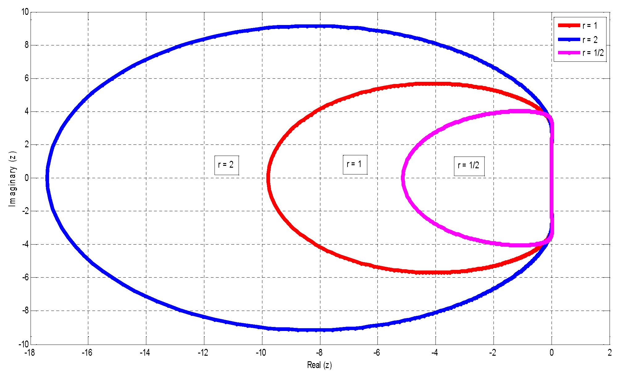
3.5. Regions of Absolute Stability

Definition 4.

[44] “If the region of absolute stability of a method contains the whole left half-plane $Re(h\lambda )<0$, such a method is referred to as A-stable”.

Figure 2 shows the regions of absolute of the NFSSA.

The region of absolute stability of the NFSSA at $r=1$, $r=2$ and $r=1/2$ is the interior of the red-, blue- and magenta-colored regions, respectively. This implies that the region of absolute stability is largest when the step-size is halved ($r=2$) followed by when the step-size remains the same ($r=1$). The smallest stability region occurs when the step-size is doubled ($r=1/2$).

Table 4. Stability intervals of the NFSSA.

Step-Size Ratio	Stability Interval
$r=1$	$\left(-9.6, 0\right)$
$r=2$	$\left(-17.2, 0\right)$
$r=1/2$	$\left(-5.0, 0\right)$

shows the stability intervals of the NFSSA at the three step-size ratios.

Table 4 clearly shows that NFSSA at $r=2$ has the largest stability interval, followed by the NFSSA at $r=1$. NFSSA at $r=1/2$ has the smallest stability interval in relation to the other two.

4. Pseudocode and Step-Size Selection for Implementation of the NFSSA

4.1. Pseudocode

To implement the newly derived NFSSA, the pseudocode for the method is briefly explained in this subsection. Finding the initial points in the starting block is the first step in the code. The value of $r$ is taken as one in the starting block (see Figure 1). The Euler method is used to determine the three additional points $x_{n-2},x_{n-1}$ and $x_n$. The starting block can be applied after the points $y_{n+1/2},y_{n+1},y_{n+3/2},y_{n+2}$ for the next block has been determined. It is important to state here that each point in the predictor and the corrector formulae can perform the computations simultaneously within the block because they are independent of each other. Therefore, the values of $y_{n+1/2},y_{n+1},y_{n+3/2},y_{n+2}$ are approximated using the predictor-corrector formulae. Let $s$ be the number of iterations needed, then the sequence of computations at a mesh point is $(PE){(CE)}^1{(CE)}^2{(CE)}^3\dots {(CE)}^s$, where $P$ and C are the predictor and corrector formulae. The function evaluation $f$ of the problem is denoted by E. The starting/back values $x_{n-2}$, $x_{n-1}$ and $x_n$ are determined using the truncated Taylor series method at $j=0,1$(otherwise called the Euler method).

Step 1: Set the following data input: initial conditions, tolerance level and step-size

Step 2: The approximate solution of the stiff system in Equation (1) is determined using the newly derived NFSSA simultaneously at points $x_{n+1/2}$, $x_{n+1}$, $x_{n+3/2}$ and $x_{n+2}$ with the solution information available at the back (previous) values $x_{n-2}$, $x_{n-1}$ and $x_n$. The initial step-size is taken as $h_{old}=h_{initial}$.

Step 3: Initiate the Euler method algorithm $y_n={\displaystyle \sum _{j=0}^1\frac{h^j{y}_{n-1}^{(j)}}{j!}}=y_{n-1}+hf\left(x_{n-1},y_{n-1}\right)$.

Step 4: Set the equations of the predictor

$$P:y_{n+1/2}^p={\displaystyle \sum _{j=0}^2{\alpha }_{n+j}{f}_{n-j}+{\alpha }_{n+1/2}{f}_{n+1/2}+{\alpha }_{n+3/2}{f}_{n+3/2}}$$

$$y_{n+1}^p={\displaystyle \sum _{j=0}^2{\beta }_{n+j}{f}_{n-j}+{\beta }_{n+1/2}{f}_{n+1/2}}+{\beta }_{n+3/2}{f}_{n+3/2}$$

$$y_{n+3/2}^p={\displaystyle \sum _{j=0}^2{\gamma }_{n+j}{f}_{n-j}+{\gamma }_{n+1/2}{f}_{n+1/2}}+{\gamma }_{n+3/2}{f}_{n+3/2}$$

$$y_{n+2}^p={\displaystyle \sum _{j=0}^2{\mu }_{n+j}{f}_{n-j}+{\mu }_{n+1/2}{f}_{n+1/2}}+{\mu }_{n+3/2}{f}_{n+3/2}$$

$$E:f_{n+1/2}^p=\left(x_{n+1/2},y_{n+1/2}^p\right)$$

$$f_{n+1}^p=\left(x_{n+1},y_{n+1}^p\right)$$

$$f_{n+3/2}^p=\left(x_{n+3/2},y_{n+3/2}^p\right)$$

$$f_{n+2}^p=\left(x_{n+2},y_{n+2}^p\right)$$

Step 5: Set the equations of the corrector

$$C:y_{n+1/2}^c={\displaystyle \sum _{j=0}^4{\phi }_{n+j}{f}_{n+2-j}+{\phi }_{n+1/2}{f}_{n+1/2}}+{\phi }_{n+3/2}{f}_{n+3/2}$$

$$y_{n+1}^c={\displaystyle \sum _{j=0}^4{\rho }_{n+j}{f}_{n+2-j}+{\rho }_{n+1/2}{f}_{n+1/2}}+{\rho }_{n+3/2}{f}_{n+3/2}$$

$$y_{n+3/2}^c={\displaystyle \sum _{j=0}^4{\zeta }_{n+j}{f}_{n+2-j}+{\zeta }_{n+1/2}{f}_{n+1/2}}+{\zeta }_{n+3/2}{f}_{n+3/2}$$

$$y_{n+2}^c={\displaystyle \sum _{j=0}^4{\omega }_{n+j}{f}_{n+2-j}+{\omega }_{n+1/2}{f}_{n+1/2}+{\omega }_{n+3/2}{f}_{n+3/2}}$$

$$E:f_{n+1/2}^c=\left(x_{n+1/2},y_{n+1/2}^c\right)$$

$$f_{n+1}^c=\left(x_{n+1},y_{n+1}^c\right)$$

$$f_{n+3/2}^c=\left(x_{n+3/2},y_{n+3/2}^c\right)$$

$$f_{n+2}^c=\left(x_{n+2},y_{n+2}^c\right)$$

Step 6: Compute the Local Truncation Error (LTE) defined by $\mathrm{LTE}=\Vert y_{n+2}-y_{n+2}^{*}\Vert$. Note that $y_{n+2}$ is the value obtained by the Euler method while $y_{n+2}^{*}$ is the value obtained by NFSSA at $x_{n+2}$.

Step 7: The solution is acceptable if LTE < TOL. At this point, maintain $(r=1)$ or double $(r=1/2)$ the previous step size. Further, proceed with the integration process using the new step size $h_{new}$ provided $h_{\mathrm{minimum}}\le h_{new}\le h_{\mathrm{maximum}}$.

Step 8: If LTE > TOL, halve the previous step size $(r=2)$ and repeat the computation using $h_{new}$ in as much as $h_{\mathrm{minimum}}\le h_{new}\le h_{\mathrm{maximum}}$.

Step 9: Stop.

4.2. Step-Size Selection

The importance of the choice of step-size cannot be overemphasized in the numerical integration of stiff differential systems [45,46]. In fact, according to study [47], one of the most vital concepts in numerical integration of systems of differential equations is step-size selection because it is not practical to use constant step size in numerical integration. Proper step-size selection enhances accuracy, reduces computation time and minimizes the number of iterations. The approximations $y_{n+1/2}$, $y_{n+1}$, $y_{n+3/2}$ and $y_{n+2}$ are successful if the LTE is less than the tolerance level. Thus, the previous step-size is maintained (that is $r=1$) or doubled (that is $r=1/2$). After a successful step, the step-size increment denoted by $h_{new}$ is given by,

$$h_{new}=\upsilon \ast h_{old}\ast \sqrt[p]{\left(\mathrm{TOL}/\mathrm{LTE}\right)}$$

(27)

where $p$ is the order of the method, $h_{old}$ is the step size of the previous block and $h_{new}$ is the step size of the current block. The safety factor $\upsilon$ ensures that the failure steps are minimized to the barest minimum.

If, however, LTE is greater than the tolerance level, then the approximations $y_{n+1/2}$, $y_{n+1}$, $y_{n+3/2}$ and $y_{n+2}$ fail. The previous step is repeated with $r=2$ (that is, halving the previous step size).

5. Numerical Examples

The following stiff differential systems shall be studied.

5.1. Problem 1

Consider the well-known highly stiff Robertson’s chemical differential system,

$$\begin{array}{l}{y}_1^{\prime }(x)=-0.04y_1(x)+{10}^4{y}_2(x)y_3(x),y_1(0)=1\\ y_2^{\prime }(x)=0.04y_1(x)-{10}^4{y}_2(x)y_3(x)-3\times {10}^7{y}_2^2(x),y_2(0)=0\\ y_3^{\prime }(x)=3\times {10}^7{y}_2^2(x),y_3(0)=0\end{array}\}$$

(28)

A lot of researchers believe that this problem is a fairly hard test problem for numerical integrators [1,48,49,50]. Hence, the need to test the performance of the proposed NFSSA on the problem in Equation (28). The problem is solved in the interval $x\in [0,40]$ and the numerical results are to be obtained by considering,

$$\left(h_{initial},\mathrm{TOL}\right)=\left({10}^{-j},{10}^{-(j+3)}\right),j=7,8,9,10$$

(29)

5.2. Problem 2

Consider the highly stiff differential system,

$$\begin{array}{l}{y}_1^{\prime }(x)=-{10}^7{y}_1(x)+0.075y_2(x),y_1(0)=1\\ y_2^{\prime }(x)=7500y_1(x)-0.075y_2(x),y_2(0)=-1\end{array}\}$$

(30)

The eigenvalues of the Jacobian of the differential system in Equation (30) are approximately ${\lambda }_1=-1.000000000562500\times {10}^6$ and ${\lambda }_2=-0.0743749995813$. The problem is solved in the range $x\in [0,40]$.

5.3. Problem 3

Consider the mildly stiff differential system,

$$\begin{array}{l}{y}_1^{\prime }(x)=y_2(x),y_1(0)=1.01\\ y_2^{\prime }(x)=-100y_1(x)-101y_2(x),y_2(0)=-2\end{array}\}$$

(31)

defined over the interval $x\in [0,20]$. The exact solution of the differential system is,

$$\begin{array}{l}{y}_1(x)=0.01e^{-100x}+e^{-x}\\ y_2(x)=-e^{-100x}-e^{-x}\end{array}\}$$

(32)

The Jacobian matrix of the differential system in Equation (31) has the eigenvalues ${\lambda }_1=-1$ and ${\lambda }_2=-100$. This problem is solved by varying the tolerances and taking $h_{initial}={10}^{-3}$. The tolerances have been selected in order to have the same number of steps for all methods considered for computation.

5.4. Problem 4

Consider the highly stiff second-order nonlinear Van der Pol equation of the form,

$$y^{″}(x)+\mu \left(1+y^2(x)\right)y^{\prime }(x)+y(x)=0,y(0)=2,y{}^{\prime }(0)=0$$

(33)

Equation (33) is transformed to its equivalent system of first-order differential equations of the form,

$$\begin{array}{l}{y}_1^{\prime }(x)=y_2(x),y_1(0)=2\\ y_2^{\prime }(x)=\left[-y_1(x)+\left(1-y_1^2(x)\right)y_2(x)\right]/\in ,y_2(0)=0\end{array}\}$$

(34)

This transformation is achieved by substituting $y_1(x)=\phi (x),y_2(x)=\mu {\phi }^{\prime }(x)$ and $x=x/\mu$, where $\in =1/{\mu }^2$ is a parameter that controls stiffness. The value of $\in =500$ and the problem is solved in the range $x\in [0,70]$ and $h=0.1$. Equation (34) is a highly stiff differential system.

6. Results and Discussion

The NFSSA derived is applied in integrating the stiff differential problems listed in Section 5. Codes were written in MATLAB R2021a (version 9.10, MathWorks, Natick, MA, USA) for the implementation of the proposed NFSSA. This is aimed at testing the computational reliability, efficiency and accuracy of the proposed algorithm.

Table 5. Numerical results for Problem 1.

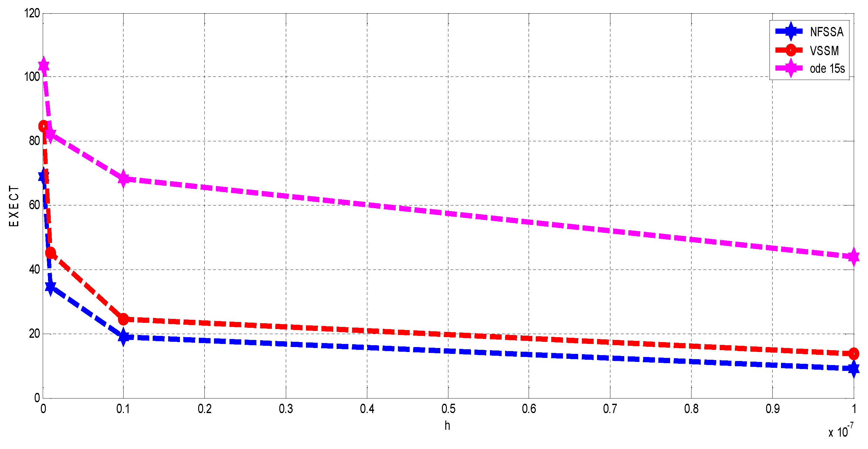
hinitial	TOL	Method	MAXERR (y1)	MAXERR (y2)	MAXERR (y3)	NST	FNE	FLS	EXECT
10−7	10−10	NFSSA	4.1983 × 10−19	3.1041 × 10−23	5.0013 × 10−19	3902	7110	00	9.05
		VSSM	4.4408 × 10−16	3.3881 × 10−21	5.5511 × 10−17	3730	14,920	00	13.88
		ode 15s	7.7561 × 10−9	5.4664 × 10−12	8.2009 × 10−10	2006	56,090	00	43.98
10−8	10−11	NFSSA	6.3923 × 10−19	1.1680 × 10−23	3.0361 × 10−19	6960	16,780	00	19.12
		VSSM	8.8817 × 10−16	1.8634 × 10−20	4.9960 × 10−16	6626	26,504	00	24.46
		ode 15s	9.5637 × 10−9	7.9259 × 10−12	8.9771 × 10−10	4344	60,020	00	68.46
10−9	10−12	NFSSA	2.5256 × 10−19	3.7445 × 10−22	1.0927 × 10−18	12,002	28,080	00	34.81
		VSSM	3.2196 × 10−15	3.2187 × 10−20	2.7755 × 10−15	11,766	47,064	00	45.10
		ode 15s	6.0929 × 10−9	4.3587 × 10−12	4.7460 × 10−10	7608	64,030	00	82.22
10−10		NFSSA	6.1523 × 10−18	4.1914 × 10−22	9.2440 × 10−17	21,228	56,024	00	69.02
		VSSM	4.3298 × 10−15	2.3716 × 10−20	8.3266 × 10−16	20,916	83,664	00	84.63
		ode 15s	7.2701 × 10−9	6.2401 × 10−12	6.4396 × 10−10	15,018	72,670	00	103.47

presents the implementation of the NFSSA on Problem 1 by taking $\left(h_{initial},\mathrm{TOL}\right)=\left({10}^{-07},{10}^{-10}\right)$, $\left({10}^{-08},{10}^{-11}\right)$, $\left({10}^{-09},{10}^{-12}\right)$ and $\left({10}^{-10},{10}^{-13}\right)$. It was observed that the NFSSA performed better than the VSSM and ode 15s in terms of maximum errors, number of steps, number of function evaluations and execution time. The efficiency curves presented in Figure 3 clearly show that the NFSSA is more efficient in terms of economy of execution time than the VSSM and the ode 15s. This implies that the NFSSA generates results faster than the two methods. It is also important to mention here that the NFSSA recorded no failed/rejected steps.

Table 6. Absolute errors for Problem 2.

X	yi	SDM	ode 15s	HSDBBDF	NFSSA
5	y1	1.9196 × 10−02	5.4044 × 10−12	1.0123 × 10−17	3.0145 × 10−19
	y2	3.1501 × 10−2	7.4701 × 10−8	3.3881 × 10−21	5.5511 × 10−17
40	y1	7.9295 × 10−10	1.9841 × 10−13	5.8776 × 10−18	7.7121 × 10−21
	y2	9.7003 × 10−6	3.9544 × 10−9	7.8381 × 10−10	5.2001 × 10−13
70	y1	1.8759 × 10−13	2.2934 × 10−14	4.0276 × 10−18	4.1291 × 10−21
	y2	9.1528 × 10−8	7.0561 × 10−10	5.3701 × 10−10	3.9866 × 10−13
100	y1	1.7835 × 10−18	6.4358 × 10−16	5.3649 × 10−19	1.9087 × 10−21
	y2	4.4647 × 10−10	3.0223 × 10−10	7.1532 × 10−11	1.2781 × 10−13

displays the performance of the NFSSA on Problem 2 in comparison with the seventh order HSDBBDF developed by [11], eleventh order SDM developed by [50] as well as the MATLAB inbuilt stiff solver, ode 15s. The problem was solved at the end points,$X=5, X=40, X=70$ and $X=100$. The results obtained showed that the NFSSA of order seven performed better than the seventh-order HSDBBDF, eleventh order SDM and the ode 15s.

The performance of the NFSSA on Problem 3 is displayed in

Table 7. Numerical results for Problem 3.

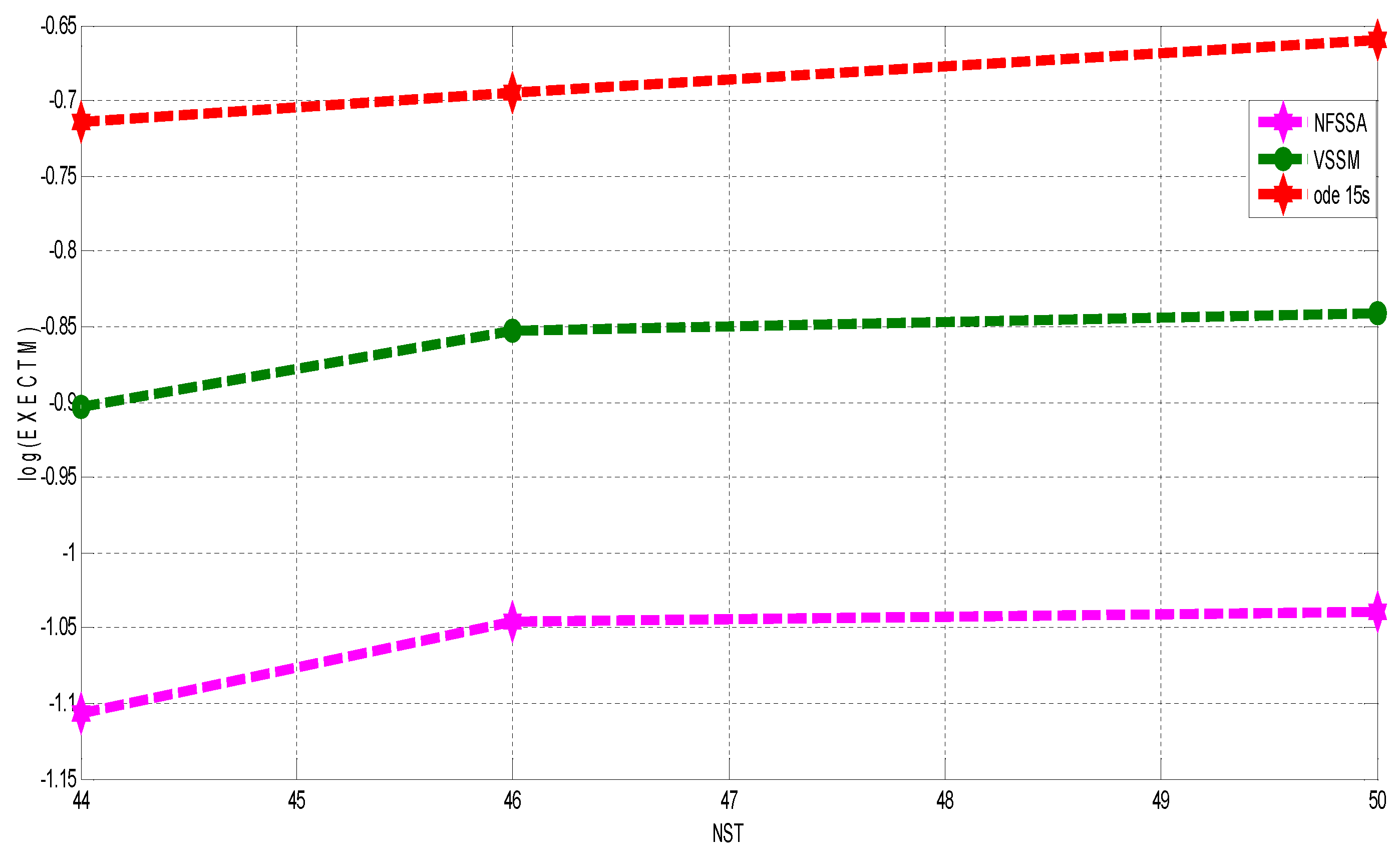
NST	Method	ABERR (y1)	ABERR (y2)	FNE	FLS	EXECTM
44	NFSSA	6.4244 × 10−15	8.1479 × 10−14	156	00	0.0781
	VSSM	3.3229 × 10−11	7.5785 × 10−11	176	00	0.1248
	ode 15s	2.2775 × 10−9	5.9313 × 10−9	198	00	0.1934
46	NFSSA	7.1241 × 10−14	9.7146 × 10−14	164	00	0.0899
	VSSM	5.7434 × 10−11	8.4486 × 10−10	184	00	0.1404
	ode 15s	4.0301 × 10−9	8.3121 × 10−9	208	00	0.2018
50	NFSSA	4.6218 × 10−12	5.0121 × 10−12	180	00	0.0914
	VSSM	2.5632 × 10−10	3.9818 × 10−10	200	00	0.1440
	ode 15s	7.1131 × 10−9	1.5736 × 10−8	228	00	0.2186

. The NFSSA performed better than the VSSM and ode 15s in terms of absolute errors, number of function evaluations and execution time. In Figure 4, the efficiency curves for Problem 3 in terms of number of steps versus execution time show that the prescribed number of steps is attained in shorter time using the NFSSA compared to both the VSSM and ode 15s. In other words, the VSSM and ode 15s take longer time to attain results with the same number of steps than the newly derived NFSSA.

The result of Problem 4 is presented in

Table 8. Approximate solution for Problem 4.

X	yi	APPSOL Using NFSSA	APPSOL Using ode 15s
1	y1	−1.8650950986	−1.8650950571
	y2	0.7524845366	0.7524845299
5	y1	1.8985234725	1.8985234421
	y2	−0.7289532611	−0.7289532451
10	y1	1.7865365303	1.7865365103
	y2	−0.8156276699	−0.8156276438
20	y1	1.5075643350	1.5075643177
	y2	−1.1911230102	−1.1911230003

. The Van der Pol problem does not have an analytical solution; thus, the approximate solution of the problem was computed using the newly derived NFSSA and compared with the approximate solution generated using the inbuilt MATLAB stiff solver, ode 15s at the end points $X=1, X=5, X=10$ and $X=20$. The results obtained clearly showed that the NFSSA is computationally reliable. The graphical plots displayed in Figure 5 further buttresses the fact that the solution curves of the NFSSA converge to those of ode 15s.

7. Conclusions

In this research, the non-fixed step-size strategy was adopted in deriving an algorithm for the numerical integration of highly stiff differential systems. The research also validated some basic properties of the new algorithm. The data presented in Table 5, Table 6, Table 7 and Table 8 validate the fact that the NFSSA is more accurate and also more efficient in terms of computational cost than the methods we compared our results with. Figure 3 and Figure 4 show the efficiency of the NFSSA while Figure 5 shows the convergence of the NFSSA. In the course of the research, it was also observed that the proposed NFSSA has a fewer number of function evaluations compared to the other methods. This explains the reason for the reduced execution time and reduced use in computer memory. Future research in this area may focus on the derivation and implementation of non-fixed (variable) step methods on large systems including oscillatory and other real-life problems.

References

- Ramos, H.; Sing, G. A note on variable step size formulation of a Simpson’s-type second derivative blocks method for solving stiff systems. Appl. Math. Lett. 2017, 64, 101–107. [Google Scholar] [CrossRef]
- Wend, V.V. Uniqueness of solution of ordinary differential equations. Am. Mon. 1967, 74, 27–33. [Google Scholar]
- Aiken, R. Stiff Computation; Oxford University Press: New York, NY, USA, 1985. [Google Scholar]
- Kin, J.; Cho, S.Y. Computational accuracy and efficiency of the time-splitting method in solving atmospheric transport/chemistry equations. Atmos. Environ. 1997, 31, 2215–2224. [Google Scholar]
- Curtiss, C.F.; Hirschfelder, J.O. Integration of stiff equations. Proc. Natl. Acad. Sci. USA 1952, 38, 235–243. [Google Scholar] [CrossRef]
- Spijker, M.N. Stiffness in numerical initial value problems. J. Comput. Appl. Math. 1996, 72, 393–406. [Google Scholar] [CrossRef]
- Hairer, E.; Wanner, G. Solving Ordinary Differential Equations II: Stiff Differential-Algebraic Problems, 2nd ed.; Springer: Berlin/Heidelberg, Germany, 1996. [Google Scholar]
- Sunday, J.; Kumleng, G.M.; Kamoh, N.M.; Kwanamu, J.A.; Skwame, Y.; Sarjiyus, O. Implicit four-point hybrid block integrator for the simulations of stiff models. J. Nig. Soc. Phys. Sci. 2022, 4, 287–296. [Google Scholar] [CrossRef]
- Shokri, A. An explicit trigonometrically fitted ten-step method with phase-lag of order infinity for the numerical solution of radial Schrodinger equation. Appl. Comput. Math. 2015, 14, 63–74. [Google Scholar]
- Shokri, A.; Saadat, H. P-stability, TF and VSDPL technique in Obrechkoff methods for the numerical solution of the Schrödinger equation. Bull. Iran. Math. Soc. 2016, 42, 687–706. [Google Scholar]
- Akinfenwa, O.A.; Abdulganiy, R.I.; Akinnukawe, B.I.; Okunuga, S.A. Seventh order hybrid block method for solution of first order stiff systems of initial value problems. J. Egypt. Math. Soc. 2020, 28, 34. [Google Scholar] [CrossRef]
- Sunday, J.; Odekunle, M.R.; Adesanya, A.O.; James, A.A. Extended block integrator for first-order stiff and oscillatory differential equations. Am. J. Comput. Appl. Math. 2013, 3, 283–290. [Google Scholar]
- Sunday, J. Optimized two-step second derivative methods for the solutions of stiff systems. J. Phys. Commun. 2022, 6, 055016. [Google Scholar] [CrossRef]
- Hashim, I.; Chowdhury, M.S.H.; Hosen, A. Solving linear and nonlinear stiff system of ordinary differential equations by multistage Adomian decomposition method. In Proceedings of the Third International Conference on Advances in Applied Science and Environmental Technology, Bangkok, Thailand, 28–29 December 2015. [Google Scholar]
- Amat, S.; Legaz, M.J.; Ruiz-Alvarez, J. On a Variational method for stiff differential equations arising from chemical kinetics. Mathematics 2019, 7, 459. [Google Scholar] [CrossRef]
- Shokri, A. The Symmetric P-Stable Hybrid Obrenchkoff Methods for the Numerical Solution of Second Order IVPs. TWMS J. Pure Appl. Math. 2012, 5, 28–35. [Google Scholar]
- Pankov, P.S.; Zheentaeva, Z.K.; Shirinov, T. Asymptotic reduction of solution space dimension for dynamical systems. TWMS J. Pure Appl. Math. 2021, 12, 243–253. [Google Scholar]
- Iskenderov, N.S.; Allahverdiyeva, S.I. An inverse boundary value problem for the boussineq-love equation with nonlocal integral condition. TWMS J. Pure Appl. Math. 2020, 11, 226–237. [Google Scholar]
- Qalandarov, A.A.; Khaldjigitov, A.A. Mathematical and numerical modeling of the coupled dynamic thermoelastic problems for isotropic bodies. TWMS J. Pure Appl. Math. 2020, 11, 119–126. [Google Scholar]
- Faydaoglu, S.; Ozis, T. Periodic solutions for certain non-smooth oscillators with high nonlinearities. Appl. Comput. Math. 2021, 20, 366–380. [Google Scholar]
- Adiguzel, R.S.; Aksoy, U.; Karapinar, E.; Erhan, I.M. On the solutions of fractional differential equations via Geraghty type hybrid contractions. Appl. Comput. Math. 2021, 20, 313–333. [Google Scholar]
- Ashyralyev, A.; Agirseven, D.; Agarwal, R.P. Stability estimates for delay parabolic differential and difference equations. Appl. Comput. Math. 2020, 19, 175–204. [Google Scholar]
- Ibrahim, Z.B.; Othman, K.I.; Suleiman, M. Variable step block backward differentiation formula for solving first order stiff ordinary differential equations. In Proceedings of the World Congress on Engineering, London, UK, 2–4 July 2007. [Google Scholar]
- Yashkun, U.; Aziz, N.H.A. A modified 3-point Adams block method of the variable step size strategy for solving neural delay differential equations. Sukkur IBA J. Comput. Math. Sci. 2019, 3, 37–45. [Google Scholar]
- Zawawi, I.S.M.; Ibrahim, Z.B.; Othman, K.I. Variable step block backward differentiation formula with independent parameter for solving stiff ordinary differential equations. J. Phys. Conf. Ser. 2021, 1988, 012031. [Google Scholar] [CrossRef]
- Abasi, N.; Suleiman, M.; Fudziah, I.; Ibrahim, Z.B.; Musa, H.; Abbasi, N. A new formula of variable step 3-point block backward differentiation formula method for solving stiff ordinary differential equations. J. Pure Appl. Math. Adv. Appl. 2014, 12, 49–76. [Google Scholar]
- Oghonyon, J.G.; Ogunniyi, P.O.; Ogbu, I.F. A computational strategy of variable step, variable order for solving stiff systems of ODEs. Int. J. Anal. Appl. 2021, 19, 929–948. [Google Scholar] [CrossRef]
- Rasedee, A.F.N.; Suleiman, M.; Ibrahim, Z.B. Solving non-stiff higher order ODEs using variable order step size backward difference directly. Math. Probl. Eng. 2014, 565137, 565137. [Google Scholar]
- Abasi, N.; Suleiman, M.; Ibrahim, Z.B.; Musa, H.; Rabiei, F. Variable step 2-point block backward differentiation formula for index-1 differential algebraic equations. Sci. Asia 2014, 40, 375–378. [Google Scholar] [CrossRef]
- Shampine, L.F. Variable order Adams codes. Comput. Math. Appl. 2002, 44, 749–761. [Google Scholar] [CrossRef]
- Rasedee, A.F.N.; Sathar, M.H.A.; Hamzah, S.R.; Ishak, N.; Wong, T.J.; Koo, L.F.; Ibrahim, S.N.I. Two-point block variable order step size multistep method for solving higher order ordinary differential equations directly. J. King Saud Univ. Sci. 2021, 33, 101376. [Google Scholar] [CrossRef]
- Mehrkanoon, S. A direct variable step block multistep method for solving general third order ordinary differential equations. Numer. Algorithms 2011, 57, 53–66. [Google Scholar] [CrossRef]
- Soomro, H.; Zainuddin, N.; Daud, H.; Sunday, J.; Jamaludin, N.; Abdullah, A.; Apriyanto, M.; Kadir, E.A. Variable step block hybrid method for stiff chemical kinetics problems. Appl. Sci. 2022, 12, 4484. [Google Scholar] [CrossRef]
- Han, Q. Variable step size Adams methods for BSDEs. J. Math. 2021, 2021, 9799627. [Google Scholar] [CrossRef]
- Ibrahim, Z.B.; Zainuddin, N.; Othman, K.I.; Suleiman, M.; Zawawi, I.S.M. Variable order block method for solving second order ordinary differential equations. Sains Malays. 2019, 48, 1761–1769. [Google Scholar] [CrossRef]
- Holsapple, R.; Iyer, R.; Doman, D. Variable step size selection methods for implicit integration schemes for ordinary differential equations. Int. J. Numer. Anal. Model. 2007, 4, 210–240. [Google Scholar]
- Oghonyon, J.G.; Okunuga, S.A.; Bishop, S.A. A variable step size block predictor-corrector method for ordinary differential equations. Asian J. Appl. Sci. 2017, 10, 96–101. [Google Scholar] [CrossRef]
- Sunday, J.; Shokri, A.; Marian, D. Variable step hybrid block method for the approximation of Kepler problem. Fractal Fract. 2022, 6, 343. [Google Scholar] [CrossRef]
- Iserles, A. A First Course in the Numerical Analysis of Differential Equations; Cambridge University Press: Cambridge, UK, 1996. [Google Scholar]
- Krogh, F.T. Algorithms for changing the step size. SIAM J. Num. Anal. 1973, 10, 949–965. [Google Scholar] [CrossRef]
- Krogh, F.T. Changing step size in the integration of differential equations using modified divided differences. In Proceedings of the Conference on the Numerical Solution of Ordinary Differential Equations, Austin, TX, USA, 20 October 1972; Bettis, D.G., Ed.; Springer: Berlin/Heidelberg, Germany, 1974; pp. 22–71. [Google Scholar] [CrossRef]
- Fatunla, S.O. Numerical integrators for stiff and highly oscillatory differential equations. Math Comput. 1980, 34, 373–390. [Google Scholar] [CrossRef]
- Dahlquist, G.G. A special stability problem for linear multistep methods. BIT Numer. Math. 1963, 3, 27–43. [Google Scholar] [CrossRef]
- Lambert, J.D. Computational Methods in Ordinary Differential Equations; John Wiley & Sons, Inc.: New York, NY, USA, 1973. [Google Scholar]
- Calvo, M.; Vigo-Aguiar, J. A note on the step size selection in Adams multistep methods. Numer. Algorithms 2001, 27, 359–366. [Google Scholar] [CrossRef]
- Arevalo, C.; Soderlind, G.; Hadjimichael, Y.; Fekete, I. Local error estimation and step size control in adaptative linear multistep methods. Numer. Algorithms 2021, 86, 537–563. [Google Scholar] [CrossRef]
- Kizilkan, G.C.; Aydin, K. Step size strategies for the numerical integration of systems of differential equations. J. Comput. Appl. Math. 2012, 236, 3805–3816. [Google Scholar] [CrossRef]
- Butcher, J.C.; Hojjati, G. Second derivative methods with Runge-Kutta stability. Numer. Algorithms 2005, 40, 415–429. [Google Scholar] [CrossRef]
- Vigo-Aguiar, J.; Ramos, H. A family of A-stable Runge-Kutta collocation methods of higher order for initial value problems. IMA J. Numer. Anal. 2007, 27, 798–817. [Google Scholar] [CrossRef]
- Yakubu, D.G.; Markus, S. Second derivative of high-order accuracy methods for the numerical integration of stiff initial value problems. Afr. Mat. 2016, 27, 963–977. [Google Scholar] [CrossRef]