
An Improved Equilibrium Optimizer with a Decreasing Equilibrium Pool

Abstract
:1. Introduction
2. Equilibrium Optimizer
2.1. Initialization
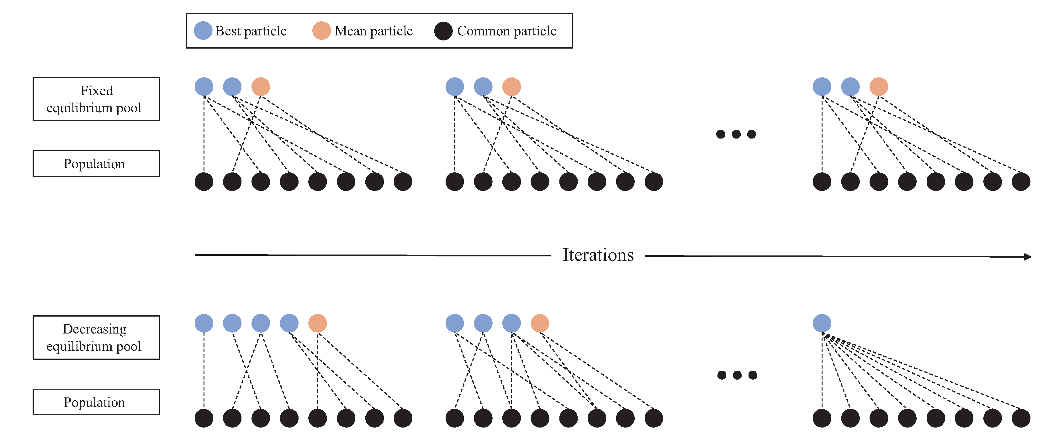
2.2. Equilibrium Pool Construction
2.3. Population Update
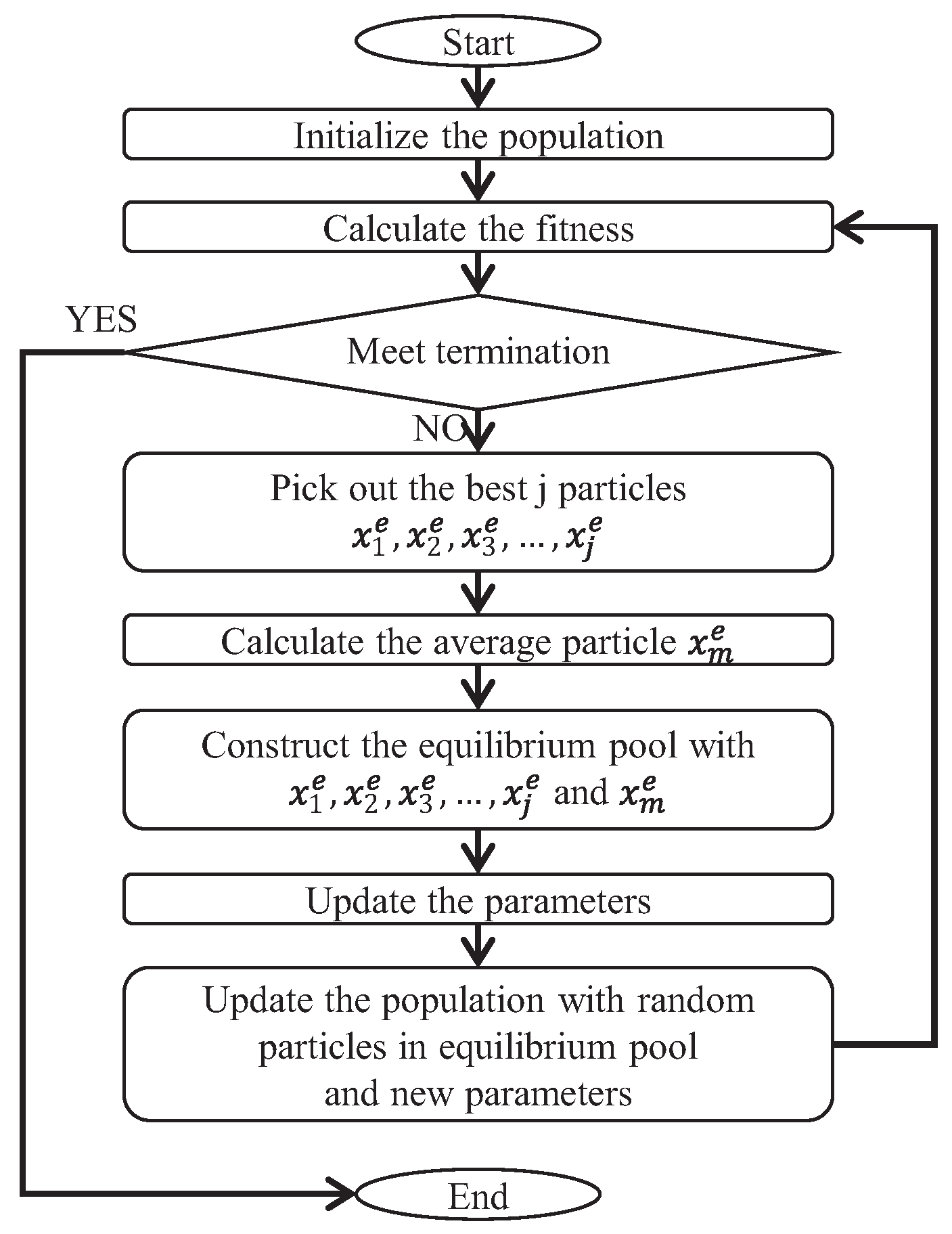
3. Improved Equilibrium Optimizer
| Algorithm 1: IEO |
 |
4. Experiment and Analysis
4.1. Experiment Setup
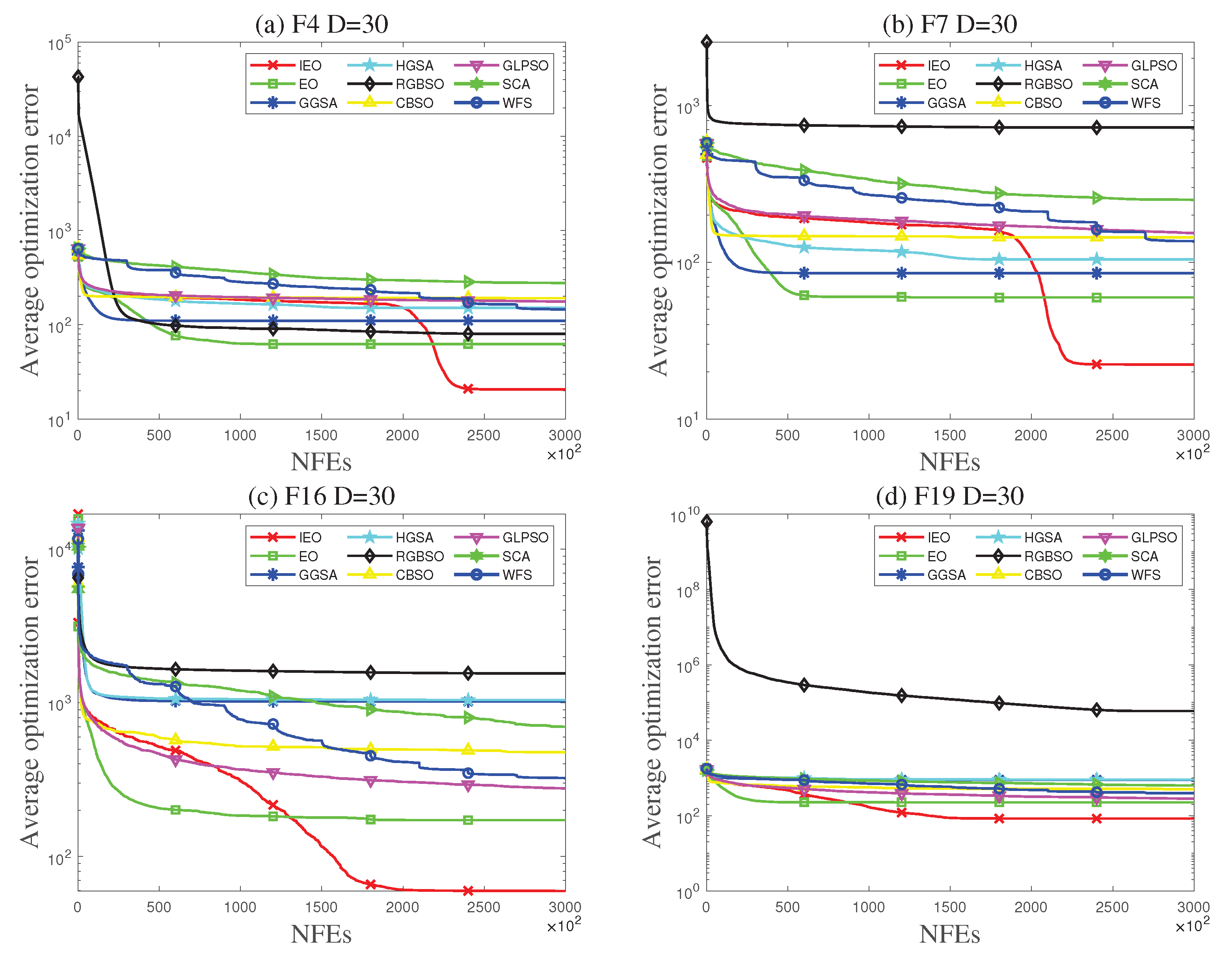
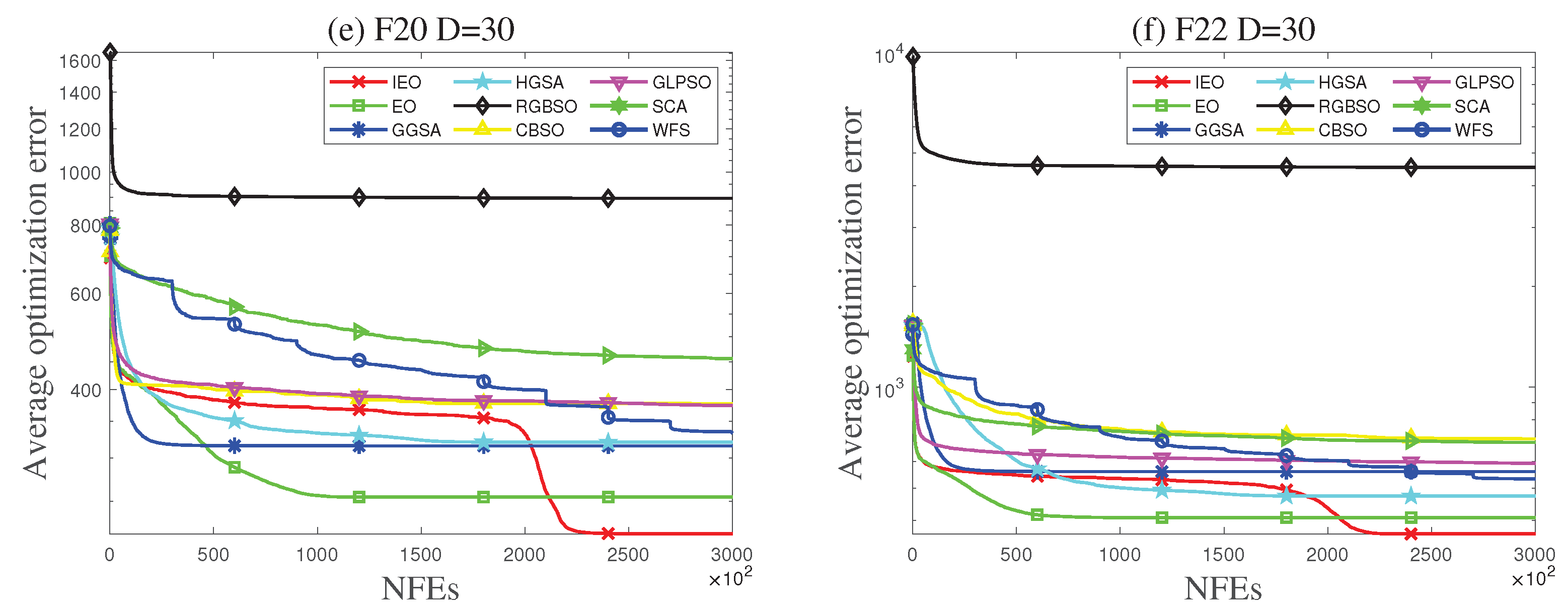
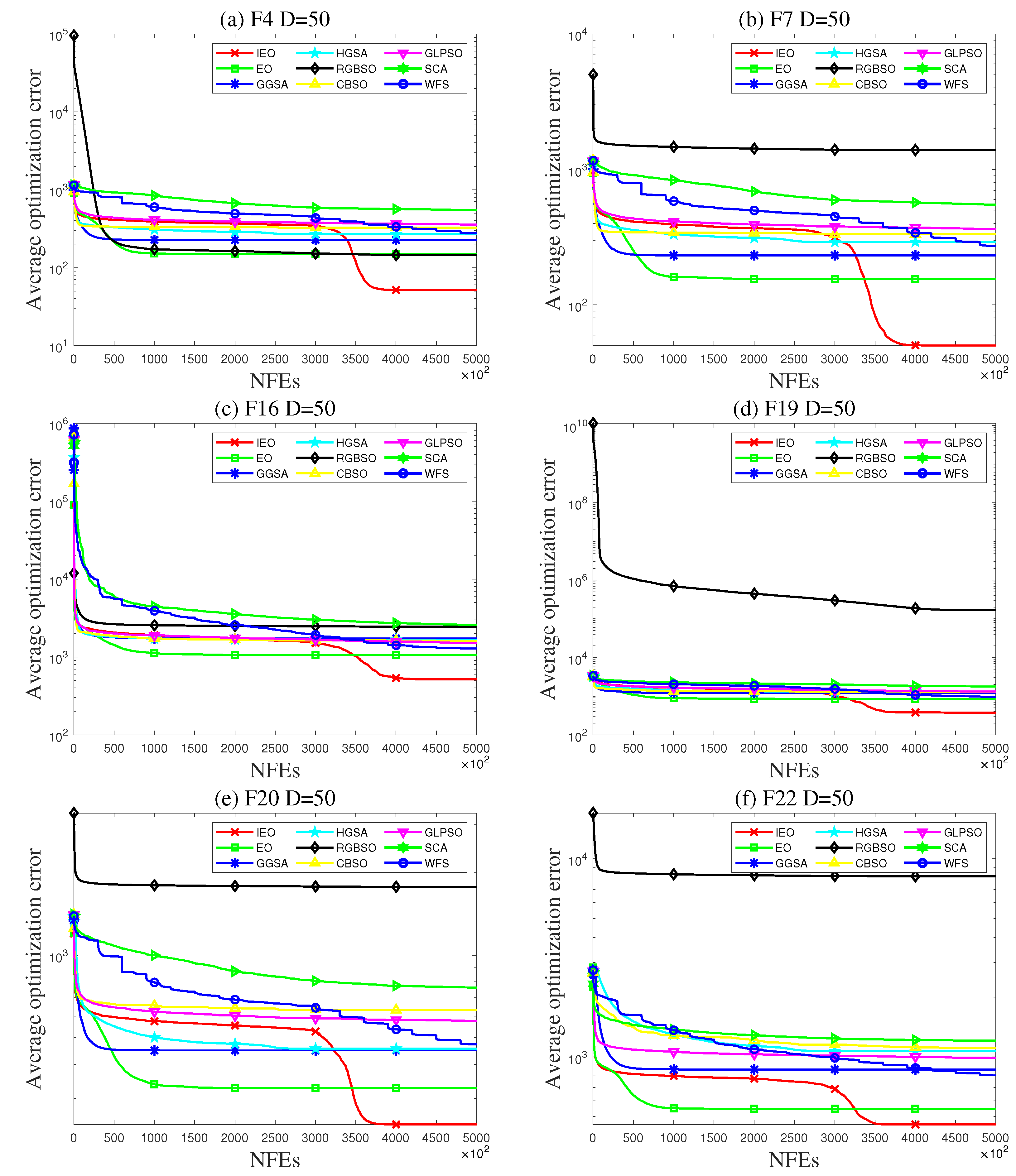
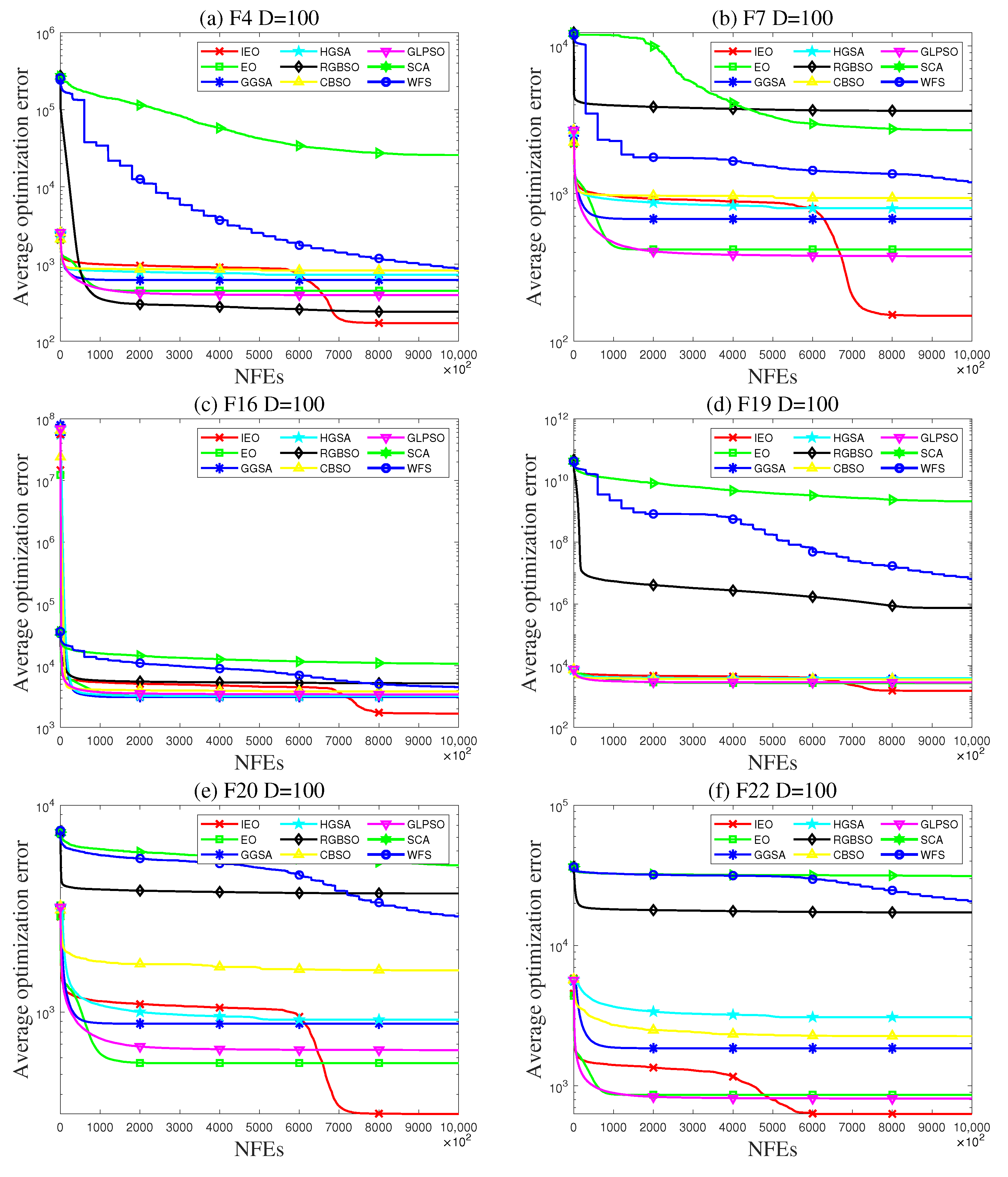
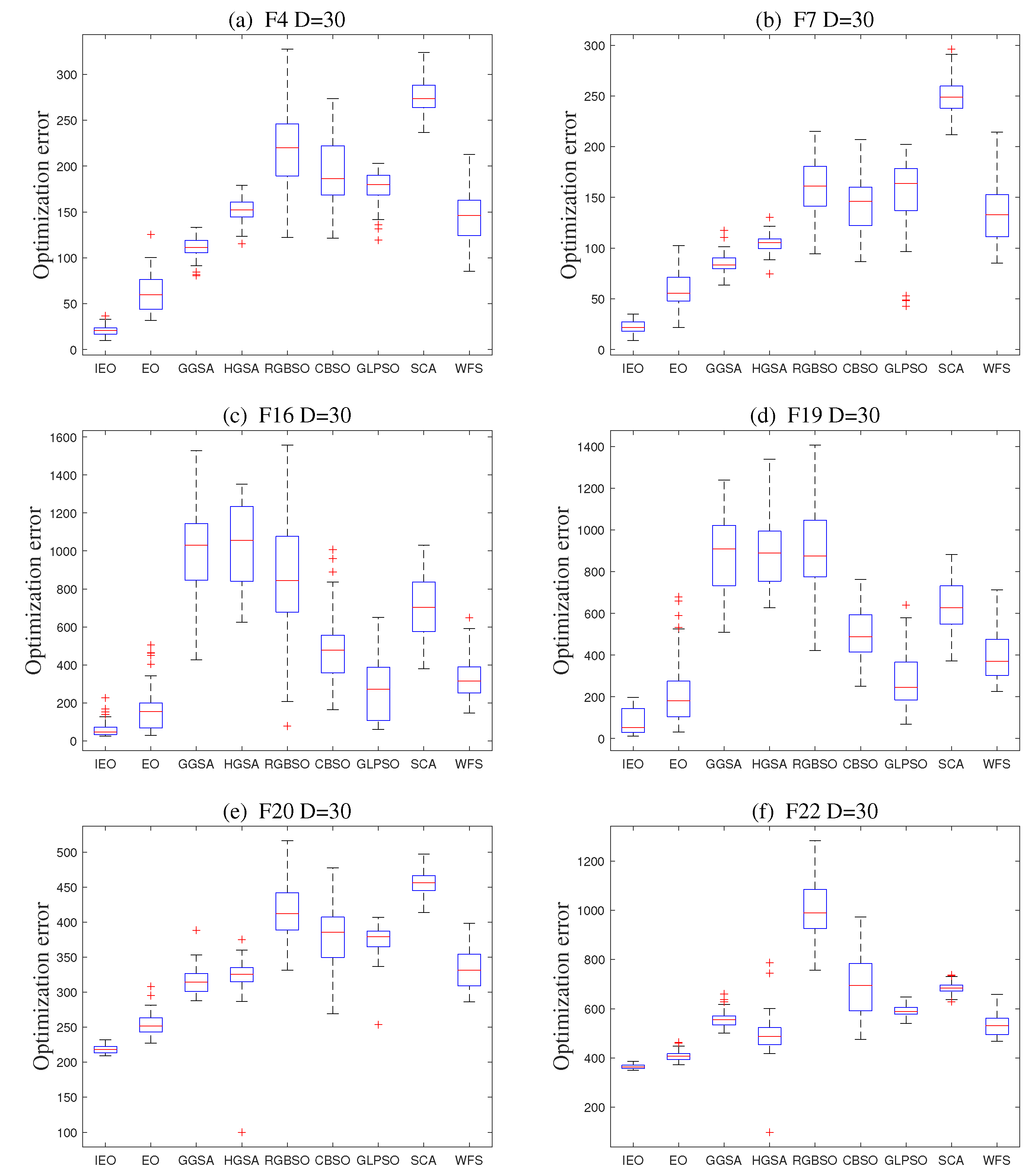
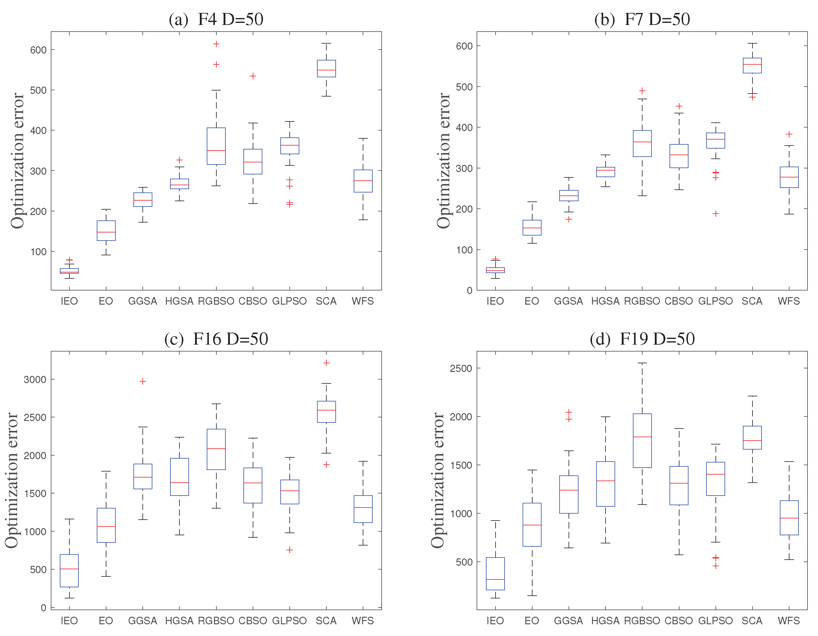
4.2. Comparison on Benchmark Functions
4.2.1. Discussion of the Parameter
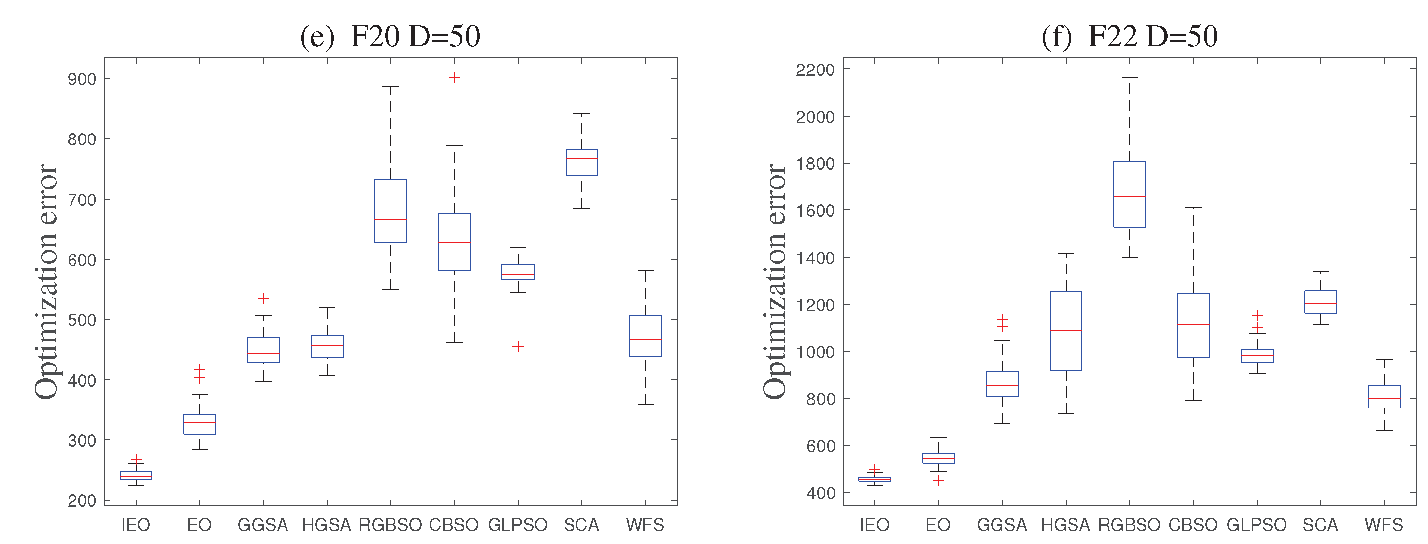
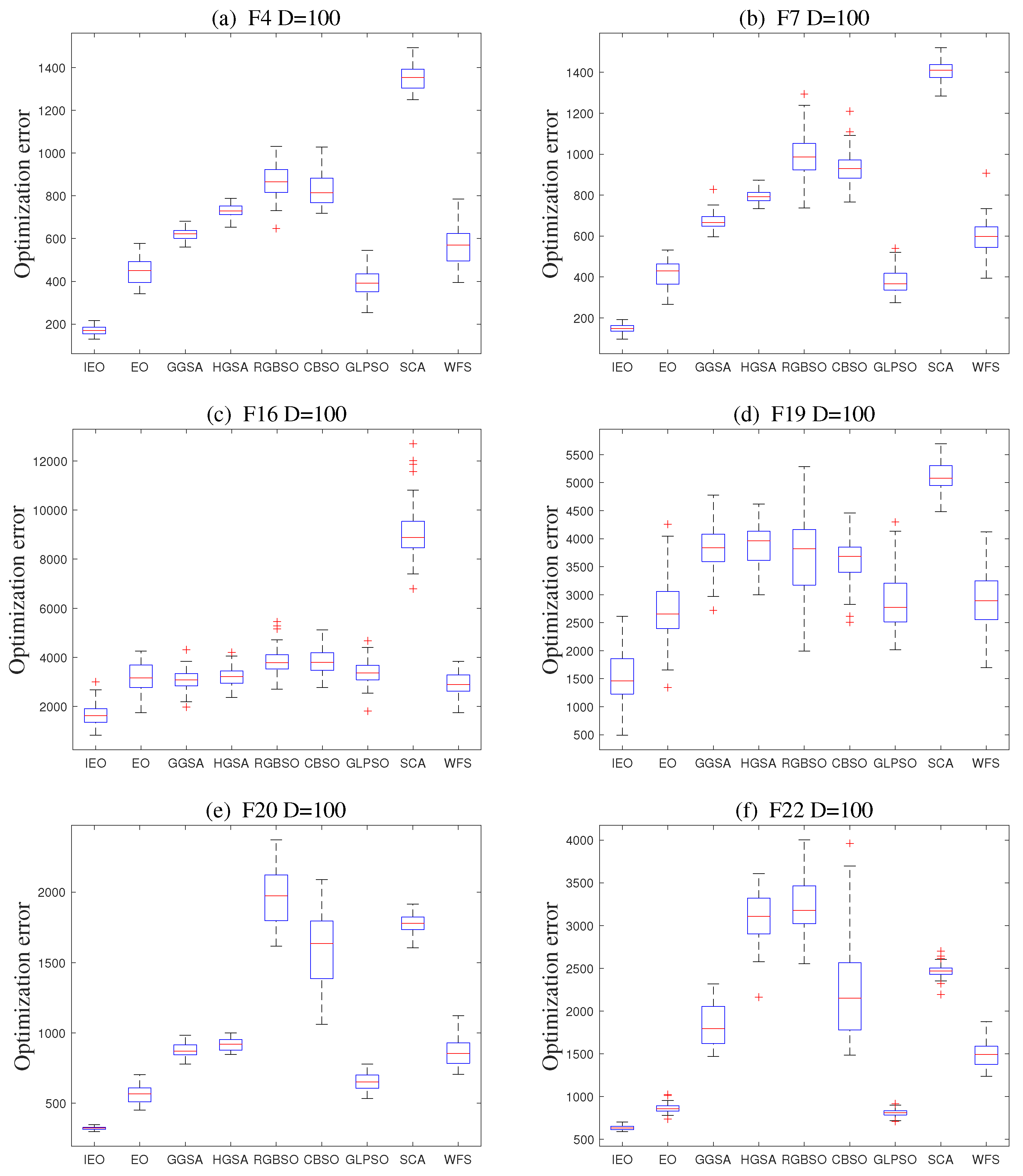
4.2.2. Experimental Data on Benchmark Functions
4.3. Comparison on Real-World Optimization Problems
4.3.1. Dynamic Economic Dispatch Problem
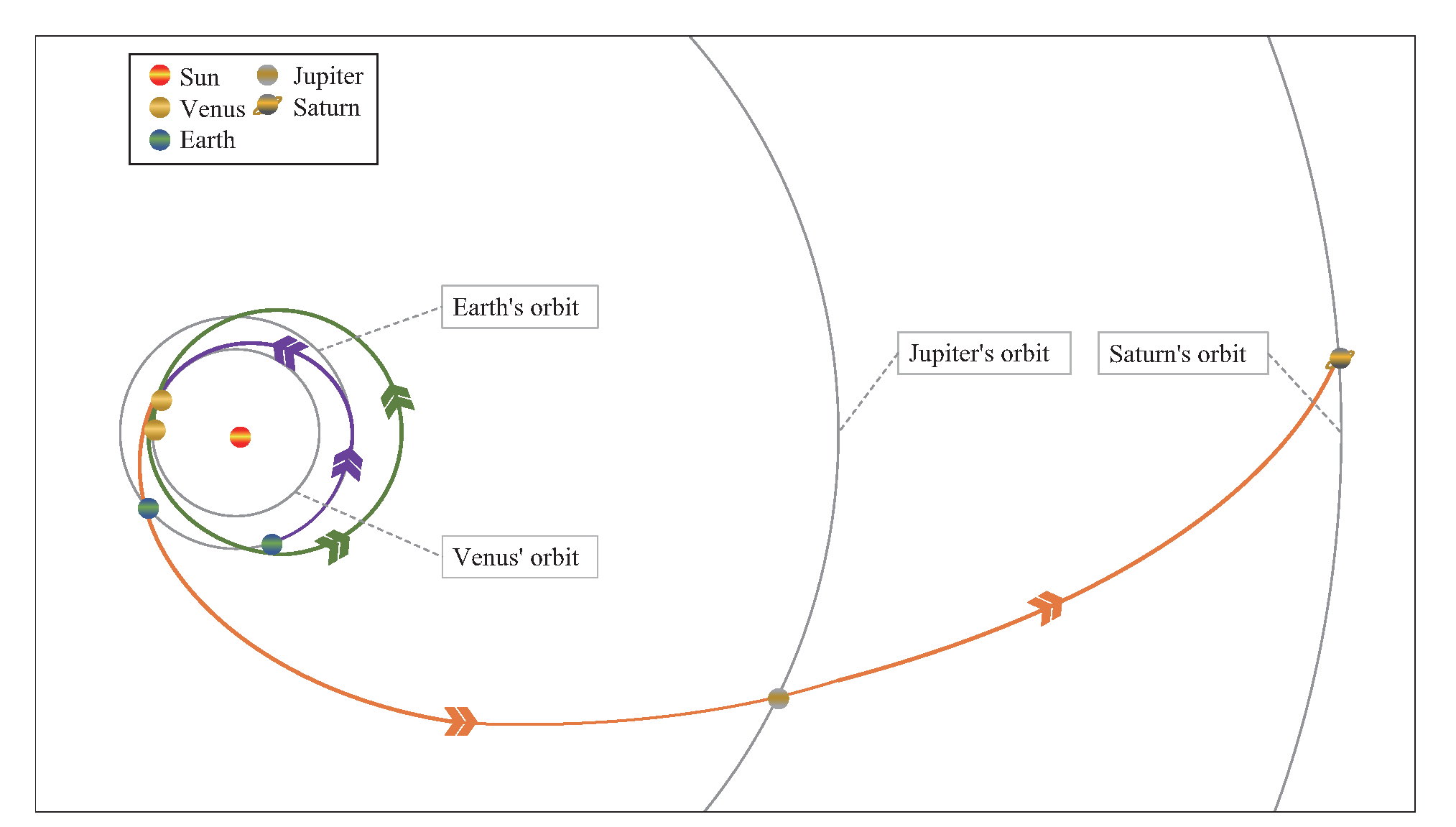
4.3.2. Spacecraft Trajectory Optimization Problem
4.3.3. Dendritic Neuron Model Training
5. Discussion and Analysis
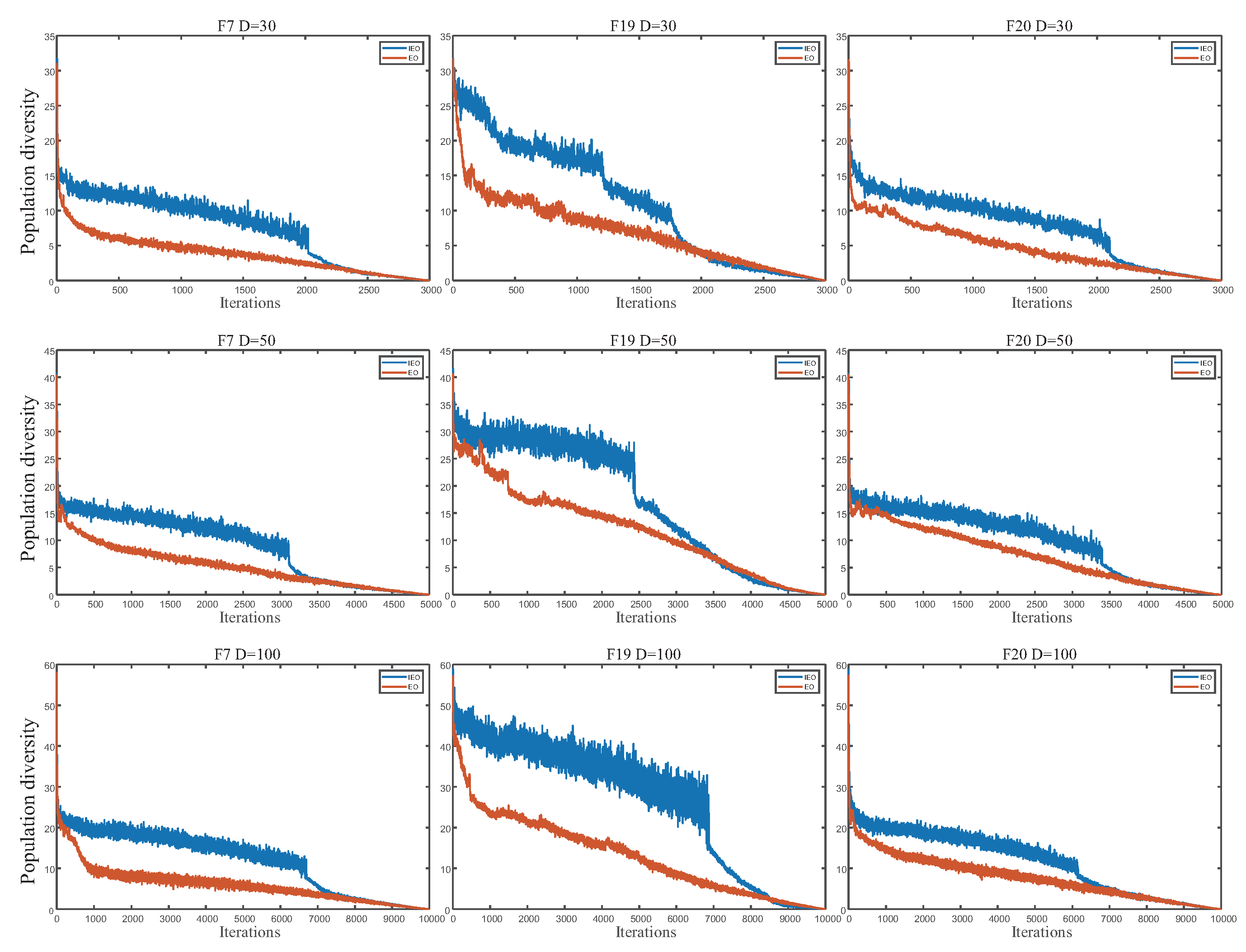
5.1. Population Diversity Discussion
5.2. Computational Complexity Analysis
6. Conclusions
Author Contributions
Funding
Institutional Review Board Statement
Informed Consent Statement
Data Availability Statement
Acknowledgments
Conflicts of Interest
Abbreviations
| Acronym | Definition |
| ANN | Artificial neural network |
| CBSO | Brain storm optimization with chaotic local search |
| CJADE | Chaotic local search-based differential evolution |
| DED | Dynamic economic dispatch |
| DNM | Dendritic neural model |
| DSM | Deep-space maneuvering |
| EO | Equilibrium optimizer |
| GGSA | Grouping gravitational search algorithm |
| GLPSO | Genetic learning particle swarm optimization |
| GSA | Gravitational search algorithm |
| HGSA | Hierarchical gravitational search algorithm |
| IEO | Improved equilibrium optimizer |
| L-SHADE | Success-history-based parameter adaptation for differential evolution using linear population size reduction |
| MNFEs | Maximum number of function evaluations |
| MGA | Multiple gravity assist |
| MHA | Metaheuristic algorithm |
| NFEs | Number of function evaluations |
| RGBSO | Random grouping brain storm optimization |
| SCA | Sine cosine algorithm |
| SED | Static economic dispatch |
| STO | Spacecraft trajectory optimization |
| WFS | Wingsuit flying search |
References
- Bottou, L.; Curtis, F.E.; Nocedal, J. Optimization methods for large-scale machine learning. Siam Rev. 2018, 60, 223–311. [Google Scholar] [CrossRef]
- Sun, S.; Cao, Z.; Zhu, H.; Zhao, J. A survey of optimization methods from a machine learning perspective. IEEE Trans. Cybern. 2019, 50, 3668–3681. [Google Scholar] [CrossRef] [Green Version]
- Abitha, R.; Vennila, S.M. A Swarm Based Symmetrical Uncertainty Feature Selection Method for Autism Spectrum Disorders. In Proceedings of the 2019 Third International Conference on Inventive Systems and Control (ICISC), Coimbatore, India, 10–11 January 2019; IEEE: Piscataway, NJ, USA, 2019; pp. 665–669. [Google Scholar]
- Das, R.; Saha, S. Gene expression classification using a fuzzy point symmetry based PSO clustering technique. In Proceedings of the 2015 Second International Conference on Soft Computing and Machine Intelligence (ISCMI), Hong Kong, 23–24 November 2015; IEEE: Piscataway, NJ, USA, 2015; pp. 69–73. [Google Scholar]
- Ren, Y.; Bai, G. Determination of optimal SVM parameters by using GA/PSO. J. Comput. 2010, 5, 1160–1168. [Google Scholar] [CrossRef]
- Panigrahi, S.; Behera, H. Time Series Forecasting Using Differential Evolution-Based ANN Modelling Scheme. Arab. J. Sci. Eng. 2020, 45, 11129–11146. [Google Scholar] [CrossRef]
- Aburomman, A.A.; Reaz, M.B.I. A novel SVM-kNN-PSO ensemble method for intrusion detection system. Appl. Soft Comput. 2016, 38, 360–372. [Google Scholar] [CrossRef]
- Hussain, K.; Mohd Salleh, M.N.; Cheng, S.; Shi, Y. Metaheuristic research: A comprehensive survey. Artif. Intell. Rev. 2019, 52, 2191–2233. [Google Scholar] [CrossRef] [Green Version]
- Gogna, A.; Tayal, A. Metaheuristics: Review and application. J. Exp. Theor. Artif. Intell. 2013, 25, 503–526. [Google Scholar] [CrossRef]
- Abdel-Basset, M.; Abdel-Fatah, L.; Sangaiah, A.K. Metaheuristic algorithms: A comprehensive review. In Computational Intelligence for Multimedia Big Data on the Cloud with Engineering Applications; Academic Press: Cambridge, MA, USA, 2018; pp. 185–231. [Google Scholar]
- Ma, L.; Huang, M.; Yang, S.; Wang, R.; Wang, X. An adaptive localized decision variable analysis approach to large-scale multiobjective and many-objective optimization. IEEE Trans. Cybern. 2021. Available online: https://ieeexplore.ieee.org/abstract/document/9332241 (accessed on 10 March 2022).
- Dokeroglu, T.; Sevinc, E.; Kucukyilmaz, T.; Cosar, A. A survey on new generation metaheuristic algorithms. Comput. Ind. Eng. 2019, 137, 106040. [Google Scholar] [CrossRef]
- Beheshti, Z.; Shamsuddin, S.M.H. A review of population-based meta-heuristic algorithms. Int. J. Adv. Soft Comput. Appl. 2013, 5, 1–35. [Google Scholar]
- Gao, S.; Wang, W.; Dai, H.; Li, F.; Tang, Z. Improved clonal selection algorithm combined with ant colony optimization. IEICE Trans. Inf. Syst. 2008, 91, 1813–1823. [Google Scholar] [CrossRef] [Green Version]
- Engin, O.; Guçlu, A. A new hybrid ant colony optimization algorithm for solving the no-wait flow shop scheduling problems. Appl. Soft Comput. 2018, 72, 166–176. [Google Scholar] [CrossRef]
- Maleki, N.; Zeinali, Y.; Niaki, S.T.A. A k-NN method for lung cancer prognosis with the use of a genetic algorithm for feature selection. Expert Syst. Appl. 2021, 164, 113981. [Google Scholar] [CrossRef]
- Ma, L.; Cheng, S.; Shi, Y. Enhancing learning efficiency of brain storm optimization via orthogonal learning design. IEEE Trans. Syst. Man Cybern. Syst. 2020, 51, 6723–6742. [Google Scholar] [CrossRef]
- Zhao, H.; Liu, K.; Li, S.; Yang, F.; Cheng, S.; Eldeeb, H.H.; Kang, J.; Xu, G. shielding optimization of ipt system based on genetic algorithm for efficiency promotion in EV wireless charging applications. IEEE Trans. Ind. Appl. 2021, 58, 1190–1200. [Google Scholar] [CrossRef]
- Zhou, M.; Long, Y.; Zhang, W.; Pu, Q.; Wang, Y.; Nie, W.; He, W. Adaptive genetic algorithm-aided neural network with channel state information tensor decomposition for indoor localization. IEEE Trans. Evol. Comput. 2021, 25, 913–927. [Google Scholar] [CrossRef]
- Cui, Z.; Zhang, J.; Wu, D.; Cai, X.; Wang, H.; Zhang, W.; Chen, J. Hybrid many-objective particle swarm optimization algorithm for green coal production problem. Inf. Sci. 2020, 518, 256–271. [Google Scholar] [CrossRef]
- Fang, S.; Wang, Y.; Wang, W.; Chen, Y.; Chen, Y. Design of permanent magnet synchronous motor servo system based on improved particle swarm optimization. IEEE Trans. Power Electron. 2022, 37, 5833–5846. [Google Scholar] [CrossRef]
- Zhang, Y.; Chen, X.; Lv, D.; Zhang, Y. Optimization of urban heat effect mitigation based on multi-type ant colony algorithm. Appl. Soft Comput. 2021, 112, 107758. [Google Scholar] [CrossRef]
- Di Caprio, D.; Ebrahimnejad, A.; Alrezaamiri, H.; Santos-Arteaga, F.J. A novel ant colony algorithm for solving shortest path problems with fuzzy arc weights. Alex. Eng. J. 2022, 61, 3403–3415. [Google Scholar] [CrossRef]
- Gao, S.; Vairappan, C.; Wang, Y.; Cao, Q.; Tang, Z. Gravitational search algorithm combined with chaos for unconstrained numerical optimization. Appl. Math. Comput. 2014, 231, 48–62. [Google Scholar] [CrossRef]
- Lei, Z.; Gao, S.; Gupta, S.; Cheng, J.; Yang, G. An aggregative learning gravitational search algorithm with self-adaptive gravitational constants. Expert Syst. Appl. 2020, 152, 113396. [Google Scholar] [CrossRef]
- Wang, Y.; Gao, S.; Zhou, M.; Yu, Y. A multi-layered gravitational search algorithm for function optimization and real-world problems. IEEE/CAA J. Autom. Sin. 2021, 8, 1–16. [Google Scholar] [CrossRef]
- Sharma, S.K.; Konki, S.K.; Khambampati, A.K.; Kim, K.Y. Bladder boundary estimation by gravitational search algorithm using electrical impedance tomography. IEEE Trans. Instrum. Meas. 2020, 69, 9657–9667. [Google Scholar] [CrossRef]
- Yu, Y.; Gao, S.; Wang, Y.; Cheng, J.; Todo, Y. ASBSO: An Improved Brain Storm Optimization With Flexible Search Length and Memory-Based Selection. IEEE Access 2018, 6, 36977–36994. [Google Scholar] [CrossRef]
- Wang, Y.; Gao, S.; Yu, Y.; Xu, Z. The discovery of population interaction with a power law distribution in brain storm optimization. Memetic Comput. 2019, 11, 65–87. [Google Scholar] [CrossRef]
- Yu, Y.; Gao, S.; Wang, Y.; Lei, Z.; Cheng, J.; Todo, Y. A multiple diversity-driven brain storm optimization algorithm with adaptive parameters. IEEE Access 2019, 7, 126871–126888. [Google Scholar] [CrossRef]
- Jiang, Y.; Chen, X.; Zheng, F.C.; Niyato, D.; You, X. Brain storm optimization-based edge caching in fog radio access networks. IEEE Trans. Veh. Technol. 2021, 70, 1807–1820. [Google Scholar] [CrossRef]
- Ma, L.; Wang, X.; Huang, M.; Lin, Z.; Tian, L.; Chen, H. Two-level master–slave RFID networks planning via hybrid multiobjective artificial bee colony optimizer. IEEE Trans. Syst. Man Cybern. Syst. 2017, 49, 861–880. [Google Scholar] [CrossRef]
- Aldhafeeri, A.; Rahmat-Samii, Y. Brain storm optimization for electromagnetic applications: Continuous and discrete. IEEE Trans. Antennas Propag. 2019, 67, 2710–2722. [Google Scholar] [CrossRef]
- Mathew, D.; Ram, J.P.; Pillai, D.S.; Kim, Y.J.; Elangovan, D.; Laudani, A.; Mahmud, A. Parameter Estimation of Organic Photovoltaic Cells–A Three-Diode Approach Using Wind-Driven Optimization Algorithm. IEEE J. Photovoltaics 2021, 12, 327–336. [Google Scholar] [CrossRef]
- Cheng, J.; Yuan, G.; Zhou, M.; Gao, S.; Huang, Z.; Liu, C. A connectivity-prediction-based dynamic clustering model for VANET in an urban scene. IEEE Internet Things J. 2020, 7, 8410–8418. [Google Scholar] [CrossRef]
- Kranina, E.I. China on the way to achieving carbon neutrality. Finans. Financ. J. 2021, 5, 51–61. [Google Scholar] [CrossRef]
- Faramarzi, A.; Heidarinejad, M.; Stephens, B.; Mirjalili, S. Equilibrium optimizer: A novel optimization algorithm. Knowl. Syst. 2020, 191, 105190. [Google Scholar] [CrossRef]
- Warn, A.; Brew, J. Mass balance. Water Res. 1980, 14, 1427–1434. [Google Scholar] [CrossRef]
- Črepinšek, M.; Liu, S.H.; Mernik, M. Exploration and exploitation in evolutionary algorithms: A survey. ACM Comput. Surv. (CSUR) 2013, 45, 1–33. [Google Scholar] [CrossRef]
- Morales-Castañeda, B.; Zaldivar, D.; Cuevas, E.; Fausto, F.; Rodríguez, A. A better balance in metaheuristic algorithms: Does it exist? Swarm Evol. Comput. 2020, 54, 100671. [Google Scholar] [CrossRef]
- Xu, Z.; Yang, H.; Li, J.; Zhang, X.; Lu, B.; Gao, S. Comparative study on single and multiple chaotic maps incorporated grey wolf optimization algorithms. IEEE Access 2021, 9, 77416–77437. [Google Scholar] [CrossRef]
- Faris, H.; Aljarah, I.; Al-Betar, M.A.; Mirjalili, S. Grey wolf optimizer: A review of recent variants and applications. Neural Comput. Appl. 2018, 30, 413–435. [Google Scholar] [CrossRef]
- Gupta, S.; Deep, K. A novel random walk grey wolf optimizer. Swarm Evol. Comput. 2019, 44, 101–112. [Google Scholar] [CrossRef]
- Sun, J.; Liu, X.; Back, T.; Xu, Z. Learning adaptive differential evolution algorithm from optimization experiences by policy gradient. IEEE Trans. Evol. Comput. 2021, 9, 77416–77437. [Google Scholar] [CrossRef]
- Li, J.; Yang, L.; Yi, J.; Yang, H.; Todo, Y.; Gao, S. A Simple but Efficient Ranking-Based Differential Evolution. IEICE Trans. Inf. Syst. 2022, 105, 189–192. [Google Scholar] [CrossRef]
- Gao, S.; Yu, Y.; Wang, Y.; Wang, J.; Cheng, J.; Zhou, M. Chaotic local search-based differential evolution algorithms for optimization. IEEE Trans. Syst. Man Cybern. Syst. 2021, 51, 3954–3967. [Google Scholar] [CrossRef]
- Tanabe, R.; Fukunaga, A.S. Improving the search performance of SHADE using linear population size reduction. In Proceedings of the 2014 IEEE Congress on Evolutionary Computation (CEC), Beijing, China, 6–11 July 2014; IEEE: Piscataway, NJ, USA, 2014; pp. 1658–1665. [Google Scholar]
- Polakova, R. L-SHADE with competing strategies applied to constrained optimization. In Proceedings of the 2017 IEEE Congress on Evolutionary Computation (CEC), Donostia-San Sebastián, Spain, Piscataway, NJ, USA, 5–8 June 2017; pp. 1683–1689. [Google Scholar]
- Yang, H.; Gao, S.; Wang, R.L.; Todo, Y. A ladder spherical evolution search algorithm. IEICE Trans. Inf. Syst. 2021, 104, 461–464. [Google Scholar] [CrossRef]
- Yang, L.; Gao, S.; Yang, H.; Cai, Z.; Lei, Z.; Todo, Y. Adaptive chaotic spherical evolution algorithm. Memetic Comput. 2021, 13, 383–411. [Google Scholar] [CrossRef]
- Shilaja, C.; Arunprasath, T. Optimal power flow using moth swarm algorithm with gravitational search algorithm considering wind power. Future Gener. Comput. Syst. 2019, 98, 708–715. [Google Scholar]
- Sabri, N.M.; Puteh, M.; Mahmood, M.R. A review of gravitational search algorithm. Int. J. Adv. Soft Comput. Appl 2013, 5, 1–39. [Google Scholar]
- Younes, Z.; Alhamrouni, I.; Mekhilef, S.; Reyasudin, M. A memory-based gravitational search algorithm for solving economic dispatch problem in micro-grid. Ain Shams Eng. J. 2021, 12, 1985–1994. [Google Scholar] [CrossRef]
- Song, Z.; Gao, S.; Yu, Y.; Sun, J.; Todo, Y. Multiple chaos embedded gravitational search algorithm. IEICE Trans. Inf. Syst. 2017, 100, 888–900. [Google Scholar] [CrossRef] [Green Version]
- Sudholt, D. The benefits of population diversity in evolutionary algorithms: A survey of rigorous runtime analyses. In Theory of Evolutionary Computation; Springer: Berlin/Heidelberg, Germany, 2020; pp. 359–404. [Google Scholar]
- Nazaroff, W.W.; Alvarez-Cohen, L. Environmental Engineering Science; John Wiley & Sons: Hoboken, NJ, USA, 2001. [Google Scholar]
- Črepinšek, M.; Mernik, M.; Liu, S.H. Analysis of exploration and exploitation in evolutionary algorithms by ancestry trees. Int. J. Innov. Comput. Appl. 2011, 3, 11–19. [Google Scholar] [CrossRef]
- Gupta, D.; Ghafir, S. An overview of methods maintaining diversity in genetic algorithms. Int. J. Emerg. Technol. Adv. Eng. 2012, 2, 56–60. [Google Scholar]
- Dowlatshahi, M.B.; Nezamabadi-Pour, H. GGSA: A grouping gravitational search algorithm for data clustering. Eng. Appl. Artif. Intell. 2014, 36, 114–121. [Google Scholar] [CrossRef]
- Wang, Y.; Yu, Y.; Gao, S.; Pan, H.; Yang, G. A hierarchical gravitational search algorithm with an effective gravitational constant. Swarm Evol. Comput. 2019, 46, 118–139. [Google Scholar] [CrossRef]
- Cao, Z.; Shi, Y.; Rong, X.; Liu, B.; Du, Z.; Yang, B. Random grouping brain storm optimization algorithm with a new dynamically changing step size. In Proceedings of the International Conference in Swarm Intelligence, Beijing, China, 25–28 June 2015; Springer: Berlin/Heidelberg, Germany, 2015; pp. 357–364. [Google Scholar]
- Yu, Y.; Gao, S.; Cheng, S.; Wang, Y.; Song, S.; Yuan, F. CBSO: A memetic brain storm optimization with chaotic local search. Memetic Comput. 2017, 10, 353–367. [Google Scholar] [CrossRef]
- Gong, Y.J.; Li, J.J.; Zhou, Y.; Li, Y.; Chung, H.S.H.; Shi, Y.H.; Zhang, J. Genetic learning particle swarm optimization. IEEE Trans. Cybern. 2015, 46, 2277–2290. [Google Scholar] [CrossRef] [PubMed] [Green Version]
- Lin, A.; Sun, W.; Yu, H.; Wu, G.; Tang, H. Global genetic learning particle swarm optimization with diversity enhancement by ring topology. Swarm Evol. Comput. 2019, 44, 571–583. [Google Scholar] [CrossRef]
- Mirjalili, S. SCA: A sine cosine algorithm for solving optimization problems. Knowl. Syst. 2016, 96, 120–133. [Google Scholar] [CrossRef]
- Singh, N.; Singh, S. A novel hybrid GWO-SCA approach for optimization problems. Eng. Sci. Technol. Int. J. 2017, 20, 1586–1601. [Google Scholar] [CrossRef]
- Covic, N.; Lacevic, B. Wingsuit flying search—A novel global optimization algorithm. IEEE Access 2020, 8, 53883–53900. [Google Scholar] [CrossRef]
- Mao, Y.; Xu, F.; Zhao, X.; Yan, X. A gearbox fault feature extraction method based on wingsuit flying search algorithm-optimized orthogonal matching pursuit with a compound time-frequency atom dictionary. J. Mech. Sci. Technol. 2021, 35, 4825–4833. [Google Scholar] [CrossRef]
- Awad, N.; Ali, M.; Liang, J.; Qu, B.; Suganthan, P. Problem definitions and evaluation criteria for the CEC 2017 special session and competition on single objective real-parameter numerical optimization. Tech. Rep. 2016. [Google Scholar]
- Bushukina, V.I. Specific Features of Renewable Energy Development in the World and Russia. Finans. Financ. J. 2021, 5, 93–107. [Google Scholar] [CrossRef]
- Xia, X.; Elaiw, A. Optimal dynamic economic dispatch of generation: A review. Electr. Power Syst. Res. 2010, 80, 975–986. [Google Scholar] [CrossRef]
- Elattar, E.E. A hybrid genetic algorithm and bacterial foraging approach for dynamic economic dispatch problem. Int. J. Electr. Power Energy Syst. 2015, 69, 18–26. [Google Scholar] [CrossRef]
- Ross, D.W.; Kim, S. Dynamic economic dispatch of generation. IEEE Trans. Power Appar. Syst. 1980, 6, 2060–2068. [Google Scholar] [CrossRef]
- Attaviriyanupap, P.; Kita, H.; Tanaka, E.; Hasegawa, J. A hybrid EP and SQP for dynamic economic dispatch with nonsmooth fuel cost function. IEEE Trans. Power Syst. 2002, 17, 411–416. [Google Scholar] [CrossRef]
- Zaman, M.; Elsayed, S.M.; Ray, T.; Sarker, R.A. Evolutionary algorithms for dynamic economic dispatch problems. IEEE Trans. Power Syst. 2015, 31, 1486–1495. [Google Scholar] [CrossRef]
- Das, S.; Suganthan, P.N. Problem definitions and evaluation criteria for CEC 2011 competition on testing evolutionary algorithms on real world optimization problems. Jadavpur Univ. Nanyang Technol. Univ. Kolkata. pp. 341–359. Available online: https://al-roomi.org/multimedia/CEC_Database/CEC2011/CEC2011_TechnicalReport.pdf (accessed on 10 March 2022).
- Rosa Sentinella, M.; Casalino, L. Cooperative evolutionary algorithm for space trajectory optimization. Celest. Mech. Dyn. Astron. 2009, 105, 211–227. [Google Scholar] [CrossRef]
- Vasile, M.; Minisci, E.; Locatelli, M. An inflationary differential evolution algorithm for space trajectory optimization. IEEE Trans. Evol. Comput. 2011, 15, 267–281. [Google Scholar] [CrossRef] [Green Version]
- Zhu, Y.; Wang, H.; Zhang, J. Spacecraft multiple-impulse trajectory optimization using differential evolution algorithm with combined mutation strategies and boundary-handling schemes. Math. Probl. Eng. 2015, 2015, 949480. [Google Scholar] [CrossRef] [Green Version]
- Darani, S.A.; Abdelkhalik, O. Space trajectory optimization using hidden genes genetic algorithms. J. Spacecr. Rocket. 2018, 55, 764–774. [Google Scholar] [CrossRef]
- Danoy, G.; Dorronsoro, B.; Bouvry, P. New state-of-the-art results for Cassini2 global trajectory optimization problem. Acta Futur. 2012, 5, 65–72. [Google Scholar]
- McCulloch, W.S.; Pitts, W. A logical calculus of the ideas immanent in nervous activity. Bull. Math. Biophys. 1943, 5, 115–133. [Google Scholar] [CrossRef]
- Rosenblatt, F. The perceptron: A probabilistic model for information storage and organization in the brain. Psychol. Rev. 1958, 65, 386. [Google Scholar] [CrossRef] [PubMed] [Green Version]
- Rumelhart, D.E.; Hinton, G.E.; Williams, R.J. Learning representations by back-propagating errors. Nature 1986, 323, 533–536. [Google Scholar] [CrossRef]
- He, H.; Gao, S.; Jin, T.; Sato, S.; Zhang, X. A seasonal-trend decomposition-based dendritic neuron model for financial time series prediction. Appl. Soft Comput. 2021, 108, 107488. [Google Scholar] [CrossRef]
- Xu, Z.; Wang, Z.; Li, J.; Jin, T.; Meng, X.; Gao, S. Dendritic neuron model trained by information feedback-enhanced differential evolution algorithm for classification. Knowl. Syst. 2021, 233, 107536. [Google Scholar] [CrossRef]
- Gao, S.; Zhou, M.; Wang, Y.; Cheng, J.; Yachi, H.; Wang, J. Dendritic neuron model with effective learning algorithms for classification, approximation, and prediction. IEEE Trans. Neural Netw. Learn. Syst. 2019, 30, 601–614. [Google Scholar] [CrossRef]
- Blake, C. UCI Repository of Machine Learning Databases. 1998. Available online: http://www.ics.uci.edu/mlearn/MLRepository.html (accessed on 10 March 2022).
- Cheng, S.; Shi, Y.; Qin, Q.; Zhang, Q.; Bai, R. Population diversity maintenance in brain storm optimization algorithm. J. Artif. Intell. Soft Comput. Res. 2014, 4, 83–97. [Google Scholar] [CrossRef] [Green Version]
- He, L.; Huang, S. An efficient krill herd algorithm for color image multilevel thresholding segmentation problem. Appl. Soft Comput. 2020, 89, 106063. [Google Scholar] [CrossRef]
- Narmatha, C.; Eljack, S.M.; Tuka, A.A.R.M.; Manimurugan, S.; Mustafa, M. A hybrid fuzzy brain-storm optimization algorithm for the classification of brain tumor MRI images. J. Ambient. Intell. Humaniz. Comput. 2020, 1–9. [Google Scholar] [CrossRef]
- Tang, L.; Wang, X. An Improved Particle Swarm Optimization Algorithm for the Hybrid Flowshop Scheduling to Minimize Total Weighted Completion Time in Process Industry. IEEE Trans. Control Syst. Technol. 2010, 18, 1303–1314. [Google Scholar] [CrossRef]
- Marichelvam, M.K.; Prabaharan, T.; Yang, X.S. A discrete firefly algorithm for the multi-objective hybrid flowshop scheduling problems. IEEE Trans. Evol. Comput. 2014, 18, 301–305. [Google Scholar] [CrossRef]
- Zhang, G.; Ma, X.; Wang, L.; Xing, K. Elite archive-assisted adaptive memetic algorithm for a realistic hybrid differentiation flowshop scheduling problem. IEEE Trans. Evol. Comput. 2022, 26, 100–114. [Google Scholar] [CrossRef]
- Moiseev, N.; Mikhaylov, A.; Varyash, I.; Saqib, A. Investigating the relation of GDP per capita and corruption index. Entrep. Sustain. Issues 2020, 8, 780. [Google Scholar] [CrossRef]
- Mutalimov, V.; Kovaleva, I.; Mikhaylov, A.; Stepanova, D. Assessing regional growth of small business in Russia. Entrep. Bus. Econ. Rev. 2021, 9, 119–133. [Google Scholar] [CrossRef]
- Matveeva, N.S. Legislative Regulation Financial Statement Preparation by Micro Entities: International Experience. Finans. Financ. J. 2021, 5, 125–138. [Google Scholar] [CrossRef]


| EO | IEO | |||||||
|---|---|---|---|---|---|---|---|---|
| - | 1/64 | 2/64 | 4/64 | 8/64 | 16/64 | 32/64 | 64/64 | |
| F1 | 3.8201E + 03 | 5.5418E + 03 | 4.2338E + 03 | 3.6199E + 03 | 4.0864E + 03 | 3.0915E + 03 | 2.3701E + 03 | 2.6264E + 03 |
| F2 | 5.0923E + 01 | 5.1493E + 02 | 4.4414E + 02 | 7.0833E + 02 | 1.7886E + 03 | 2.7093E + 03 | 4.1765E + 03 | 6.1440E + 03 |
| F3 | 8.4854E + 01 | 7.9318E + 01 | 8.8599E + 01 | 8.8394E + 01 | 9.1840E + 01 | 9.7913E + 01 | 1.0293E + 02 | 9.2376E + 01 |
| F4 | 6.2329E + 01 | 3.2797E + 01 | 2.4340E + 01 | 2.0598E + 01 | 1.8921E + 01 | 1.6563E + 01 | 1.7072E + 01 | 1.7498E + 01 |
| F5 | 7.8148E - 03 | 1.2427E - 03 | 2.7188E - 05 | 3.6545E - 06 | 7.8805E - 07 | 3.2616E - 06 | 2.0632E - 06 | 8.9197E - 06 |
| F6 | 9.0975E + 01 | 5.9836E + 01 | 5.2140E + 01 | 4.9094E + 01 | 4.6480E + 01 | 4.5556E + 01 | 4.5263E + 01 | 4.7800E + 01 |
| F7 | 5.9598E + 01 | 3.5167E + 01 | 2.7320E + 01 | 2.2282E + 01 | 2.0348E + 01 | 2.1128E + 01 | 1.9193E + 01 | 1.8427E + 01 |
| F8 | 8.9579E + 00 | 1.0975E + 00 | 2.6256E - 01 | 5.6830E - 02 | 4.7921E - 02 | 7.1135E - 02 | 1.9538E - 02 | 1.9572E - 02 |
| F9 | 3.2687E + 03 | 2.8894E + 03 | 2.9942E + 03 | 2.6223E + 03 | 2.6354E + 03 | 2.7862E + 03 | 2.8170E + 03 | 2.8198E + 03 |
| F10 | 5.0615E + 01 | 4.3128E + 01 | 4.5207E + 01 | 3.6975E + 01 | 2.7141E + 01 | 3.0934E + 01 | 4.0697E + 01 | 4.4323E + 01 |
| F11 | 8.2715E + 04 | 7.4212E + 04 | 5.0784E + 04 | 3.8584E + 04 | 4.8540E + 04 | 1.0787E + 05 | 2.3749E + 05 | 2.3750E + 05 |
| F12 | 1.9975E + 04 | 3.2302E + 04 | 1.8792E + 04 | 1.9494E + 04 | 1.8296E + 04 | 1.9240E + 04 | 2.1367E + 04 | 2.3298E + 04 |
| F13 | 5.5963E + 03 | 1.1393E + 04 | 9.0457E + 03 | 1.1780E + 04 | 1.5284E + 04 | 3.2635E + 04 | 3.2804E + 04 | 2.7922E + 04 |
| F14 | 5.7821E + 03 | 7.9448E + 03 | 3.5718E + 03 | 2.2946E + 03 | 2.6415E + 03 | 2.3349E + 03 | 1.8578E + 03 | 3.4511E + 03 |
| F15 | 6.0395E + 02 | 3.4120E + 02 | 1.3976E + 02 | 1.0357E + 02 | 1.5098E + 02 | 1.4537E + 02 | 1.1289E + 02 | 1.8262E + 02 |
| F16 | 1.7232E + 02 | 1.2927E + 02 | 8.1288E + 01 | 5.9592E + 01 | 4.9528E + 01 | 9.6392E + 01 | 1.1846E + 02 | 1.4430E + 02 |
| F17 | 1.4721E + 05 | 1.6634E + 05 | 1.7057E + 05 | 2.1896E + 05 | 2.1736E + 05 | 3.3293E + 05 | 3.0677E + 05 | 2.9835E + 05 |
| F18 | 7.2785E + 03 | 9.2941E + 03 | 4.7905E + 03 | 6.2676E + 03 | 4.6660E + 03 | 3.3079E + 03 | 2.9895E + 03 | 4.1361E + 03 |
| F19 | 2.2445E + 02 | 1.3147E + 02 | 1.0329E + 02 | 8.3284E + 01 | 1.0319E + 02 | 9.4965E + 01 | 1.1937E + 02 | 1.2740E + 02 |
| F20 | 2.5448E + 02 | 2.3210E + 02 | 2.2283E + 02 | 2.1799E + 02 | 2.1482E + 02 | 2.1219E + 02 | 2.1296E + 02 | 2.1334E + 02 |
| F21 | 1.0827E + 03 | 6.5254E + 02 | 2.4967E + 02 | 2.5006E + 02 | 1.7928E + 02 | 1.0000E + 02 | 1.5333E + 02 | 1.4876E + 02 |
| F22 | 4.0823E + 02 | 3.8659E + 02 | 3.7385E + 02 | 3.6466E + 02 | 3.6114E + 02 | 3.6058E + 02 | 3.6207E + 02 | 3.6691E + 02 |
| F23 | 4.7204E + 02 | 4.5447E + 02 | 4.4314E + 02 | 4.3535E + 02 | 4.3182E + 02 | 4.3105E + 02 | 4.3167E + 02 | 4.3573E + 02 |
| F24 | 3.8681E + 02 | 3.8741E + 02 | 3.8692E + 02 | 3.8616E + 02 | 3.8678E + 02 | 3.8649E + 02 | 3.8704E + 02 | 3.8767E + 02 |
| F25 | 1.4754E + 03 | 1.2563E + 03 | 1.0936E + 03 | 1.0218E + 03 | 1.0104E + 03 | 1.0194E + 03 | 1.0443E + 03 | 1.0683E + 03 |
| F26 | 5.1388E + 02 | 5.1375E + 02 | 5.1058E + 02 | 5.1130E + 02 | 5.0935E + 02 | 5.0991E + 02 | 5.0735E + 02 | 5.0456E + 02 |
| F27 | 3.5272E + 02 | 3.6856E + 02 | 3.4200E + 02 | 3.3158E + 02 | 3.3168E + 02 | 3.4552E + 02 | 3.9282E + 02 | 4.0875E + 02 |
| F28 | 5.9015E + 02 | 5.3879E + 02 | 5.0609E + 02 | 4.8857E + 02 | 4.8070E + 02 | 4.9965E + 02 | 5.1428E + 02 | 5.1134E + 02 |
| F29 | 5.8267E + 03 | 7.0522E + 03 | 4.8887E + 03 | 4.0673E + 03 | 4.1686E + 03 | 4.1643E + 03 | 3.9059E + 03 | 9.9617E + 03 |
| w/t/l | - | 15/9/5 | 16/11/2 | 22/4/3 | 21/4/4 | 18/6/5 | 18/4/7 | 14/6/9 |
| IEO | EO | GGSA | HGSA | RGBSO | ||||||||||
|---|---|---|---|---|---|---|---|---|---|---|---|---|---|---|
| Mean | Std | Mean | Std | w/t/l | Mean | Std | w/t/l | Mean | Std | w/t/l | Mean | Std | w/t/l | |
| F1 | 3.6199E + 03 | 3.5151E + 03 | 3.8201E + 03 | 4.2554E + 03 | ≈ | 1.8451E + 03 | 9.6247E + 02 | ≈ | 2.8402E + 03 | 2.5681E + 03 | ≈ | 2.5390E + 03 | 2.7946E + 03 | − |
| F2 | 7.0833E + 02 | 5.6770E + 02 | 5.0923E + 01 | 8.1049E + 01 | − | 5.8158E + 04 | 6.5549E + 03 | + | 4.4830E + 04 | 3.5988E + 03 | + | 1.8937E + 00 | 1.3501E + 01 | − |
| F3 | 8.8394E + 01 | 1.7620E + 01 | 8.4854E + 01 | 1.9797E + 01 | ≈ | 1.3046E + 02 | 1.9501E + 01 | + | 1.1909E + 02 | 2.1410E + 00 | + | 8.0098E + 01 | 3.1504E + 01 | − |
| F4 | 2.0598E + 01 | 5.0532E + 00 | 6.2329E + 01 | 2.0740E + 01 | + | 1.1040E + 02 | 1.1557E + 01 | + | 1.5123E + 02 | 1.3641E + 01 | + | 2.1843E + 02 | 4.3945E + 01 | + |
| F5 | 3.6500E - 06 | 5.8693E - 06 | 7.8150E - 03 | 3.6618E - 02 | + | 7.9756E + 00 | 3.9141E + 00 | + | 8.9075E + 00 | 5.8584E + 00 | + | 5.7551E + 01 | 1.0113E + 01 | + |
| F6 | 4.9094E + 01 | 6.9315E + 00 | 9.0975E + 01 | 1.8113E + 01 | + | 3.7082E + 01 | 1.9707E + 00 | − | 4.0258E + 01 | 2.3497E + 00 | − | 7.2251E + 02 | 1.5304E + 02 | + |
| F7 | 2.2282E + 01 | 5.9701E + 00 | 5.9598E + 01 | 1.6208E + 01 | + | 8.5254E + 01 | 1.1052E + 01 | + | 1.0424E + 02 | 8.5489E + 00 | + | 1.5915E + 02 | 2.8817E + 01 | + |
| F8 | 5.6830E - 02 | 1.4176E - 01 | 8.9579E + 00 | 2.3641E + 01 | + | 1.1100E - 13 | 1.5919E - 14 | + | 5.4700E - 14 | 5.7356E - 14 | ≈ | 3.9163E + 03 | 1.1922E + 03 | + |
| F9 | 2.6223E + 03 | 5.4304E + 02 | 3.2687E + 03 | 7.9000E + 02 | + | 3.3096E + 03 | 3.8220E + 02 | + | 3.1832E + 03 | 4.9038E + 02 | + | 4.4514E + 03 | 5.6905E + 02 | + |
| F10 | 3.6975E + 01 | 2.9939E + 01 | 5.0615E + 01 | 3.7544E + 01 | + | 1.4518E + 02 | 3.2270E + 01 | + | 9.6132E + 01 | 2.9653E + 01 | + | 1.5266E + 02 | 5.2182E + 01 | + |
| F11 | 3.8584E + 04 | 1.8746E + 04 | 8.2715E + 04 | 9.5750E + 04 | + | 9.5566E + 05 | 2.9198E + 06 | + | 1.3525E + 05 | 7.0641E + 04 | + | 8.8516E + 05 | 6.1130E + 05 | + |
| F12 | 1.9494E + 04 | 1.8469E + 04 | 1.9975E + 04 | 1.8023E + 04 | ≈ | 1.7726E + 04 | 4.8150E + 03 | ≈ | 1.2462E + 04 | 5.2102E + 03 | ≈ | 5.6412E + 04 | 2.4798E + 04 | + |
| F13 | 1.1780E + 04 | 1.1625E + 04 | 5.5963E + 03 | 3.8567E + 03 | − | 2.3074E + 05 | 9.8247E + 04 | + | 7.2466E + 03 | 5.0104E + 03 | ≈ | 3.5561E + 03 | 3.0188E + 03 | − |
| F14 | 2.2946E + 03 | 2.5517E + 03 | 5.7821E + 03 | 8.7840E + 03 | + | 2.8972E + 03 | 1.5176E + 03 | + | 7.4044E + 02 | 5.7494E + 02 | − | 3.6757E + 04 | 3.4187E + 04 | + |
| F15 | 1.0357E + 02 | 1.6551E + 02 | 6.0395E + 02 | 2.8590E + 02 | + | 1.1826E + 03 | 2.2901E + 02 | + | 1.1531E + 03 | 1.8358E + 02 | + | 1.5567E + 03 | 4.2614E + 02 | + |
| F16 | 5.9592E + 01 | 4.1194E + 01 | 1.7232E + 02 | 1.2639E + 02 | + | 1.0199E + 03 | 2.0203E + 02 | + | 1.0441E + 03 | 1.8983E + 02 | + | 8.6791E + 02 | 3.1558E + 02 | + |
| F17 | 2.1896E + 05 | 2.0519E + 05 | 1.4721E + 05 | 1.3929E + 05 | − | 1.5767E + 05 | 7.4682E + 04 | ≈ | 6.1170E + 04 | 1.9302E + 04 | − | 1.1082E + 05 | 7.3741E + 04 | − |
| F18 | 6.2676E + 03 | 8.6774E + 03 | 7.2785E + 03 | 1.1474E + 04 | ≈ | 4.2492E + 03 | 1.4513E + 03 | ≈ | 2.8665E + 03 | 1.1666E + 03 | − | 5.9510E + 04 | 2.5619E + 04 | + |
| F19 | 8.3284E + 01 | 5.7696E + 01 | 2.2445E + 02 | 1.6266E + 02 | + | 8.9584E + 02 | 1.7032E + 02 | + | 9.0784E + 02 | 1.9053E + 02 | + | 8.9560E + 02 | 2.1587E + 02 | + |
| F20 | 2.1799E + 02 | 5.8174E + 00 | 2.5448E + 02 | 1.6317E + 01 | + | 3.1568E + 02 | 1.8209E + 01 | + | 3.2085E + 02 | 3.5376E + 01 | + | 4.1761E + 02 | 3.9279E + 01 | + |
| F21 | 2.5006E + 02 | 6.1378E + 02 | 1.0827E + 03 | 1.6526E + 03 | + | 1.0000E + 02 | 1.4750E - 10 | + | 1.9106E + 02 | 6.4388E + 02 | + | 4.5386E + 03 | 1.6627E + 03 | + |
| F22 | 3.6466E + 02 | 8.6511E + 00 | 4.0823E + 02 | 2.0902E + 01 | + | 5.5997E + 02 | 3.5956E + 01 | + | 4.7313E + 02 | 1.2753E + 02 | + | 1.0049E + 03 | 1.2095E + 02 | + |
| F23 | 4.3535E + 02 | 5.6508E + 00 | 4.7204E + 02 | 1.7450E + 01 | + | 5.0816E + 02 | 3.3266E + 01 | + | 5.1817E + 02 | 3.9012E + 01 | + | 1.1547E + 03 | 1.0207E + 02 | + |
| F24 | 3.8616E + 02 | 1.6961E + 00 | 3.8681E + 02 | 2.3189E + 00 | + | 4.2705E + 02 | 1.2163E + 01 | + | 3.9169E + 02 | 8.5953E + 00 | + | 3.9042E + 02 | 1.2946E + 01 | ≈ |
| F25 | 1.0218E + 03 | 6.5066E + 01 | 1.4754E + 03 | 4.1166E + 02 | + | 3.6445E + 02 | 5.8097E + 02 | − | 2.5294E + 02 | 4.9913E + 01 | − | 6.0681E + 03 | 1.0408E + 03 | + |
| F26 | 5.1130E + 02 | 9.6133E + 00 | 5.1388E + 02 | 8.9043E + 00 | + | 6.7680E + 02 | 4.5096E + 01 | + | 5.5523E + 02 | 2.2742E + 01 | + | 1.2333E + 03 | 2.5234E + 02 | + |
| F27 | 3.3158E + 02 | 5.1621E + 01 | 3.5272E + 02 | 5.0946E + 01 | + | 4.2941E + 02 | 2.2637E + 01 | + | 3.0973E + 02 | 2.6779E + 01 | − | 3.4336E + 02 | 5.7683E + 01 | ≈ |
| F28 | 4.8857E + 02 | 7.4136E + 01 | 5.9015E + 02 | 1.4017E + 02 | + | 1.4059E + 03 | 2.2830E + 02 | + | 1.1974E + 03 | 2.1161E + 02 | + | 1.6752E + 03 | 3.4528E + 02 | + |
| F29 | 4.0673E + 03 | 2.4775E + 03 | 5.8267E + 03 | 3.6953E + 03 | + | 4.0222E + 04 | 1.5936E + 04 | + | 7.4280E + 03 | 1.7065E + 03 | + | 2.1671E + 05 | 1.6109E + 05 | + |
| 22/4/3 | 23/4/2 | 19/4/6 | 22/2/5 | |||||||||||
| Mean | Std | Mean | Std | w/t/l | Mean | Std | w/t/l | Mean | Std | w/t/l | Mean | Std | w/t/l | |
| F1 | 3.6199E + 03 | 3.5151E + 03 | 3.4547E + 03 | 2.8831E + 03 | ≈ | 9.8546E + 04 | 4.7405E + 05 | ≈ | 1.2300E+10 | 1.8861E + 09 | + | 7.0600E + 08 | 3.3218E + 08 | + |
| F2 | 7.0833E + 02 | 5.6770E + 02 | 2.8012E + 00 | 3.0761E + 00 | − | 2.1908E + 04 | 5.1452E + 03 | + | 3.5239E + 04 | 6.4800E + 03 | + | 1.4999E + 04 | 4.3852E + 03 | + |
| F3 | 8.8394E + 01 | 1.7620E + 01 | 9.2781E + 01 | 1.9072E + 01 | ≈ | 2.9136E + 02 | 9.2432E + 01 | + | 9.4294E + 02 | 2.4076E + 02 | + | 2.4543E + 02 | 5.2236E + 01 | + |
| F4 | 2.0598E + 01 | 5.0532E + 00 | 1.9165E + 02 | 3.6548E + 01 | + | 1.7613E + 02 | 1.9160E + 01 | + | 2.7811E + 02 | 2.0565E + 01 | + | 1.4475E + 02 | 2.9777E + 01 | + |
| F5 | 3.6500E - 06 | 5.8693E - 06 | 4.9007E + 01 | 7.8882E + 00 | + | 5.0867E + 00 | 2.0623E + 00 | + | 4.9563E + 01 | 5.7827E + 00 | + | 2.5497E + 01 | 5.9342E + 00 | + |
| F6 | 4.9094E + 01 | 6.9315E + 00 | 4.2736E + 02 | 9.7850E + 01 | + | 1.6204E + 02 | 5.4063E + 01 | + | 4.2351E + 02 | 3.8486E + 01 | + | 2.3444E + 02 | 3.7474E + 01 | + |
| F7 | 2.2282E + 01 | 5.9701E + 00 | 1.4414E + 02 | 2.8042E + 01 | + | 1.5346E + 02 | 3.8183E + 01 | + | 2.5010E + 02 | 1.8564E + 01 | + | 1.3497E + 02 | 3.0966E + 01 | + |
| F8 | 5.6830E - 02 | 1.4176E - 01 | 3.1811E + 03 | 7.3984E + 02 | + | 1.4093E + 01 | 9.2473E + 00 | + | 4.3222E + 03 | 9.1786E + 02 | + | 1.7691E + 03 | 1.1261E + 03 | + |
| F9 | 2.6223E + 03 | 5.4304E + 02 | 4.2537E + 03 | 5.5536E + 02 | + | 6.5419E + 03 | 3.3508E + 02 | + | 7.2163E + 03 | 2.8934E + 02 | + | 4.5989E + 03 | 6.4967E + 02 | + |
| F10 | 3.6975E + 01 | 2.9939E + 01 | 1.3272E + 02 | 4.7078E + 01 | + | 1.3224E + 02 | 6.0069E + 01 | + | 1.0336E + 03 | 4.3619E + 02 | + | 3.2107E + 02 | 6.9430E + 01 | + |
| F11 | 3.8584E + 04 | 1.8746E + 04 | 1.9301E + 06 | 1.1817E + 06 | + | 7.8399E + 06 | 1.3277E + 07 | + | 1.0400E + 09 | 2.3930E + 08 | + | 9.8021E + 07 | 7.8849E + 07 | + |
| F12 | 1.9494E + 04 | 1.8469E + 04 | 5.1355E + 04 | 3.4987E + 04 | + | 5.5042E + 04 | 2.2968E + 05 | − | 4.1700E + 08 | 1.8508E + 08 | + | 7.4742E + 05 | 8.1424E + 05 | + |
| F13 | 1.1780E + 04 | 1.1625E + 04 | 2.0972E + 03 | 2.3221E + 03 | − | 3.5265E + 04 | 8.1008E + 04 | + | 1.3739E + 05 | 7.2931E + 04 | + | 7.6726E + 03 | 7.8219E + 03 | − |
| F14 | 2.2946E + 03 | 2.5517E + 03 | 2.6543E + 04 | 1.5272E + 04 | + | 8.4908E + 03 | 8.3134E + 03 | + | 1.2024E + 07 | 9.8201E + 06 | + | 1.5527E + 05 | 1.5805E + 05 | + |
| F15 | 1.0357E + 02 | 1.6551E + 02 | 1.1887E + 03 | 2.7675E + 02 | + | 1.3590E + 03 | 2.0549E + 02 | + | 2.0011E + 03 | 2.1658E + 02 | + | 9.7168E + 02 | 2.4958E + 02 | + |
| F16 | 5.9592E + 01 | 4.1194E + 01 | 4.7674E + 02 | 1.8831E + 02 | + | 2.7774E + 02 | 1.6462E + 02 | + | 6.9894E + 02 | 1.6541E + 02 | + | 3.2220E + 02 | 1.0678E + 02 | + |
| F17 | 2.1896E + 05 | 2.0519E + 05 | 8.6355E + 04 | 4.5953E + 04 | − | 6.9469E + 05 | 7.4988E + 05 | + | 3.3325E + 06 | 1.5395E + 06 | + | 2.1557E + 05 | 1.4811E + 05 | ≈ |
| F18 | 6.2676E + 03 | 8.6774E + 03 | 8.7262E + 04 | 5.2872E + 04 | + | 9.5482E + 03 | 1.3932E + 04 | ≈ | 2.4667E + 07 | 1.3341E + 07 | + | 1.1035E + 06 | 1.1299E + 06 | + |
| F19 | 8.3284E + 01 | 5.7696E + 01 | 5.0451E + 02 | 1.2919E + 02 | + | 2.7930E + 02 | 1.3767E + 02 | + | 6.3236E + 02 | 1.2777E + 02 | + | 3.9184E + 02 | 1.0843E + 02 | + |
| F20 | 2.1799E + 02 | 5.8174E + 00 | 3.7707E + 02 | 4.3225E + 01 | + | 3.7432E + 02 | 2.3446E + 01 | + | 4.5630E + 02 | 1.6812E + 01 | + | 3.3317E + 02 | 2.8495E + 01 | + |
| F21 | 2.5006E + 02 | 6.1378E + 02 | 3.1234E + 03 | 2.1178E + 03 | + | 1.0209E + 02 | 2.3186E + 00 | + | 5.8758E + 03 | 2.5111E + 03 | + | 3.0270E + 02 | 8.4357E + 01 | + |
| F22 | 3.6466E + 02 | 8.6511E + 00 | 7.0083E + 02 | 1.2602E + 02 | + | 5.9302E + 02 | 2.0985E + 01 | + | 6.8450E + 02 | 2.3934E + 01 | + | 5.3104E + 02 | 3.9876E + 01 | + |
| F23 | 4.3535E + 02 | 5.6508E + 00 | 7.2306E + 02 | 1.2555E + 02 | + | 6.5646E + 02 | 2.1803E + 01 | + | 7.6405E + 02 | 2.4139E + 01 | + | 5.7911E + 02 | 3.6609E + 01 | + |
| F24 | 3.8616E + 02 | 1.6961E + 00 | 3.8961E + 02 | 8.8160E + 00 | ≈ | 4.3297E + 02 | 2.1262E + 01 | + | 7.0532E + 02 | 7.4080E + 01 | + | 5.2346E + 02 | 3.6169E + 01 | + |
| F25 | 1.0218E + 03 | 6.5066E + 01 | 3.6956E + 03 | 2.0393E + 03 | + | 2.9447E + 03 | 9.3611E + 02 | + | 4.3330E + 03 | 3.1722E + 02 | + | 2.5369E + 03 | 7.0180E + 02 | + |
| F26 | 5.1130E + 02 | 9.6133E + 00 | 6.7133E + 02 | 1.5932E + 02 | + | 6.6664E + 02 | 2.1532E + 01 | + | 7.0512E + 02 | 4.1231E + 01 | + | 6.1876E + 02 | 3.0913E + 01 | + |
| F27 | 3.3158E + 02 | 5.1621E + 01 | 3.8304E + 02 | 4.5887E + 01 | + | 5.4646E + 02 | 7.7220E + 01 | + | 1.0195E + 03 | 1.1502E + 02 | + | 6.3251E + 02 | 7.8679E + 01 | + |
| F28 | 4.8857E + 02 | 7.4136E + 01 | 1.3243E + 03 | 2.8811E + 02 | + | 8.6819E + 02 | 1.7833E + 02 | + | 1.7531E + 03 | 2.5222E + 02 | + | 1.0053E + 03 | 1.4405E + 02 | + |
| F29 | 4.0673E + 03 | 2.4775E + 03 | 3.9254E + 05 | 2.1093E + 05 | + | 9.1695E + 04 | 1.5387E + 05 | + | 6.6719E + 07 | 2.4207E + 07 | + | 6.8953E + 06 | 5.6303E + 06 | + |
| 23/3/3 | 26/2/1 | 29/0/0 | 27/1/1 |
| IEO | EO | GGSA | HGSA | RGBSO | ||||||||||
|---|---|---|---|---|---|---|---|---|---|---|---|---|---|---|
| Mean | Std | Mean | Std | w/t/l | Mean | Std | w/t/l | Mean | Std | w/t/l | Mean | Std | w/t/l | |
| F1 | 1.5311E + 03 | 2.1089E + 03 | 2.8318E + 03 | 2.7107E + 03 | + | 8.1505E + 02 | 1.1902E + 03 | ≈ | 7.9448E + 02 | 1.1149E + 03 | ≈ | 2.3789E + 03 | 3.4021E + 03 | ≈ |
| F2 | 1.1263E + 04 | 3.3268E + 03 | 2.8438E + 03 | 2.2159E + 03 | − | 1.3567E + 05 | 1.0190E + 04 | + | 1.1802E + 05 | 9.5141E + 03 | + | 1.7085E + 03 | 3.1764E + 03 | − |
| F3 | 6.9262E + 01 | 5.1900E + 01 | 8.6346E + 01 | 4.3053E + 01 | + | 1.8517E + 02 | 5.4256E + 01 | + | 1.9578E + 02 | 3.9702E + 01 | + | 1.4475E + 02 | 5.6851E + 01 | + |
| F4 | 5.1383E + 01 | 1.0053E + 01 | 1.5076E + 02 | 2.8656E + 01 | + | 2.2679E + 02 | 2.0587E + 01 | + | 2.6760E + 02 | 2.0650E + 01 | + | 3.6480E + 02 | 7.3741E + 01 | + |
| F5 | 2.3217E - 05 | 2.9363E - 05 | 1.3231E - 01 | 2.7165E - 01 | + | 2.4551E + 01 | 4.6891E + 00 | + | 2.3622E + 01 | 4.3942E + 00 | + | 6.1796E + 01 | 5.6440E + 00 | + |
| F6 | 8.9595E + 01 | 1.1126E + 01 | 1.9324E + 02 | 3.7980E + 01 | + | 6.5646E + 01 | 2.8082E + 00 | − | 7.0971E + 01 | 4.0368E + 00 | − | 1.3907E + 03 | 2.7022E + 02 | + |
| F7 | 5.0186E + 01 | 1.0946E + 01 | 1.5495E + 02 | 2.4796E + 01 | + | 2.3216E + 02 | 2.0943E + 01 | + | 2.9176E + 02 | 1.5818E + 01 | + | 3.6140E + 02 | 5.5489E + 01 | + |
| F8 | 8.1466E - 01 | 1.7331E + 00 | 1.8562E + 02 | 3.6280E + 02 | + | 6.5047E + 02 | 4.5085E + 02 | + | 1.1331E + 01 | 8.0126E + 01 | − | 1.1631E + 04 | 2.2277E + 03 | + |
| F9 | 4.9947E + 03 | 7.8524E + 02 | 6.1778E + 03 | 9.8142E + 02 | + | 5.8562E + 03 | 5.2612E + 02 | + | 5.7472E + 03 | 5.3555E + 02 | + | 7.6524E + 03 | 7.8010E + 02 | + |
| F10 | 3.1614E + 01 | 3.2042E + 00 | 1.2871E + 02 | 6.0573E + 01 | + | 4.0265E + 02 | 8.6827E + 01 | + | 1.2616E + 02 | 1.3519E + 01 | + | 2.0207E + 02 | 5.2416E + 01 | + |
| F11 | 7.2344E + 05 | 3.9616E + 05 | 8.9088E + 05 | 6.6327E + 05 | ≈ | 1.4256E + 06 | 3.6763E + 05 | + | 8.3355E + 05 | 3.7484E + 05 | ≈ | 3.7723E + 06 | 1.6649E + 06 | + |
| F12 | 4.0820E + 03 | 5.0743E + 03 | 7.0713E + 03 | 6.3861E + 03 | + | 1.3334E + 04 | 2.0854E + 03 | + | 5.6931E + 02 | 6.3584E + 02 | − | 7.8496E + 04 | 5.1728E + 04 | + |
| F13 | 3.8673E + 04 | 3.5577E + 04 | 5.1641E + 04 | 4.4116E + 04 | + | 7.8635E + 04 | 3.4919E + 04 | + | 2.2901E + 04 | 1.2824E + 04 | − | 2.5919E + 04 | 2.0255E + 04 | − |
| F14 | 1.1740E + 04 | 6.7497E + 03 | 1.2340E + 04 | 7.6100E + 03 | ≈ | 7.2377E + 03 | 2.0667E + 03 | − | 7.8448E + 03 | 1.7914E + 03 | − | 3.1964E + 04 | 1.6977E + 04 | + |
| F15 | 6.2370E + 02 | 2.7447E + 02 | 1.2528E + 03 | 3.8490E + 02 | + | 1.7589E + 03 | 3.0075E + 02 | + | 1.8275E + 03 | 3.0475E + 02 | + | 2.4551E + 03 | 5.0773E + 02 | + |
| F16 | 5.1489E + 02 | 2.5757E + 02 | 1.0606E + 03 | 3.1414E + 02 | + | 1.7329E + 03 | 3.0440E + 02 | + | 1.6705E + 03 | 3.0949E + 02 | + | 2.0775E + 03 | 3.4784E + 02 | + |
| F17 | 6.0450E + 05 | 2.8371E + 05 | 2.9733E + 05 | 1.9233E + 05 | − | 8.7793E + 05 | 6.7728E + 05 | + | 1.8151E + 05 | 6.7786E + 04 | − | 1.2329E + 05 | 7.0267E + 04 | − |
| F18 | 2.1759E + 04 | 1.2094E + 04 | 1.7492E + 04 | 1.3755E + 04 | − | 1.4687E + 04 | 2.7956E + 03 | − | 1.4233E + 04 | 3.3363E + 03 | − | 1.7090E + 05 | 6.3585E + 04 | + |
| F19 | 3.7736E + 02 | 2.0103E + 02 | 8.5430E + 02 | 3.1313E + 02 | + | 1.2186E + 03 | 2.8644E + 02 | + | 1.3147E + 03 | 3.1073E + 02 | + | 1.7775E + 03 | 3.7329E + 02 | + |
| F20 | 2.4096E + 02 | 9.6413E + 00 | 3.2797E + 02 | 2.8137E + 01 | + | 4.4946E + 02 | 3.0677E + 01 | + | 4.5614E + 02 | 2.6590E + 01 | + | 6.8585E + 02 | 8.1442E + 01 | + |
| F21 | 4.9011E + 03 | 1.8469E + 03 | 6.6503E + 03 | 9.7776E + 02 | + | 7.7292E + 03 | 4.7552E + 02 | + | 7.9016E + 03 | 5.1888E + 02 | + | 8.1619E + 03 | 8.8037E + 02 | + |
| F22 | 4.5500E + 02 | 1.3867E + 01 | 5.4712E + 02 | 3.4378E + 01 | + | 8.6327E + 02 | 9.3925E + 01 | + | 1.0709E + 03 | 1.9643E + 02 | + | 1.6931E + 03 | 2.0448E + 02 | + |
| F23 | 5.2300E + 02 | 1.0887E + 01 | 6.1229E + 02 | 2.7051E + 01 | + | 8.2711E + 02 | 4.5751E + 01 | + | 8.8663E + 02 | 4.8946E + 01 | + | 1.8208E + 03 | 1.9817E + 02 | + |
| F24 | 5.6810E + 02 | 2.2904E + 01 | 5.4884E + 02 | 3.6187E + 01 | − | 6.5579E + 02 | 2.6512E + 01 | + | 5.8126E + 02 | 1.4932E + 01 | + | 5.4576E + 02 | 4.2036E + 01 | − |
| F25 | 1.3522E + 03 | 1.0061E + 02 | 2.3819E + 03 | 4.2440E + 02 | + | 3.1675E + 02 | 1.1965E + 02 | − | 3.0000E + 02 | 7.5964E - 13 | − | 1.1242E + 04 | 1.2418E + 03 | + |
| F26 | 5.8967E + 02 | 4.4291E + 01 | 6.3278E + 02 | 5.5208E + 01 | + | 1.3409E + 03 | 1.6470E + 02 | + | 1.4008E + 03 | 2.7882E + 02 | + | 2.8731E + 03 | 5.5545E + 02 | + |
| F27 | 4.9820E + 02 | 2.5442E + 01 | 4.9363E + 02 | 2.3803E + 01 | ≈ | 6.2778E + 02 | 8.2392E + 01 | + | 5.0229E + 02 | 2.1101E + 01 | + | 5.0109E + 02 | 2.1552E + 01 | + |
| F28 | 4.9978E + 02 | 1.0608E + 02 | 9.4849E + 02 | 3.2370E + 02 | + | 2.2300E + 03 | 2.8897E + 02 | + | 1.7059E + 03 | 2.7060E + 02 | + | 2.7013E + 03 | 4.7793E + 02 | + |
| F29 | 8.5568E + 05 | 1.0185E + 05 | 1.0347E + 06 | 2.0391E + 05 | + | 3.0024E + 07 | 4.6679E + 06 | + | 1.3401E + 06 | 9.6083E + 04 | + | 8.9103E + 06 | 1.1678E + 06 | + |
| 22/3/4 | 24/1/4 | 19/2/8 | 24/1/4 | |||||||||||
| Mean | Std | Mean | Std | w/t/l | Mean | Std | w/t/l | Mean | Std | w/t/l | Mean | Std | w/t/l | |
| F1 | 1.5311E + 03 | 2.1089E + 03 | 6.1453E + 03 | 5.6080E + 03 | + | 6.1377E + 06 | 4.0451E + 07 | + | 3.8443E+10 | 5.6635E + 09 | + | 1.6722E + 09 | 5.8565E + 08 | + |
| F2 | 1.1263E + 04 | 3.3268E + 03 | 5.5073E + 01 | 2.3696E + 01 | − | 7.8274E + 04 | 1.1009E + 04 | + | 1.0058E + 05 | 1.5734E + 04 | + | 3.3961E + 04 | 5.7518E + 03 | + |
| F3 | 6.9262E + 01 | 5.1900E + 01 | 1.7370E + 02 | 5.0161E + 01 | + | 8.6434E + 02 | 2.4895E + 02 | + | 5.6612E + 03 | 1.3537E + 03 | + | 4.7246E + 02 | 1.1917E + 02 | + |
| F4 | 5.1383E + 01 | 1.0053E + 01 | 3.2583E + 02 | 5.2614E + 01 | + | 3.5662E + 02 | 4.1859E + 01 | + | 5.5115E + 02 | 2.9196E + 01 | + | 2.7539E + 02 | 4.7818E + 01 | + |
| F5 | 2.3217E - 05 | 2.9363E - 05 | 5.7724E + 01 | 6.9034E + 00 | + | 1.4716E + 01 | 2.9611E + 00 | + | 6.8656E + 01 | 4.9617E + 00 | + | 3.1695E + 01 | 8.1165E + 00 | + |
| F6 | 8.9595E + 01 | 1.1126E + 01 | 9.1815E + 02 | 1.4937E + 02 | + | 3.6769E + 02 | 8.1704E + 01 | + | 9.0661E + 02 | 6.4475E + 01 | + | 4.3104E + 02 | 6.0698E + 01 | + |
| F7 | 5.0186E + 01 | 1.0946E + 01 | 3.3282E + 02 | 4.6484E + 01 | + | 3.6202E + 02 | 3.8549E + 01 | + | 5.5121E + 02 | 3.0426E + 01 | + | 2.7269E + 02 | 4.1814E + 01 | + |
| F8 | 8.1466E - 01 | 1.7331E + 00 | 9.8839E + 03 | 1.6464E + 03 | + | 1.4885E + 03 | 1.1040E + 03 | + | 2.0795E + 04 | 3.7093E + 03 | + | 7.8349E + 03 | 4.1955E + 03 | + |
| F9 | 4.9947E + 03 | 7.8524E + 02 | 7.3650E + 03 | 8.4749E + 02 | + | 1.2306E + 04 | 4.4125E + 02 | + | 1.3345E + 04 | 4.1019E + 02 | + | 8.5816E + 03 | 1.0360E + 03 | + |
| F10 | 3.1614E + 01 | 3.2042E + 00 | 2.0338E + 02 | 4.7596E + 01 | + | 7.2701E + 02 | 6.0065E + 02 | + | 4.8016E + 03 | 1.2095E + 03 | + | 6.7360E + 02 | 1.1938E + 02 | + |
| F11 | 7.2344E + 05 | 3.9616E + 05 | 1.5017E + 07 | 9.5050E + 06 | + | 1.2508E + 08 | 3.1452E + 08 | + | 1.1488E+10 | 2.6297E + 09 | + | 3.3153E + 08 | 1.7748E + 08 | + |
| F12 | 4.0820E + 03 | 5.0743E + 03 | 6.3678E + 04 | 3.7539E + 04 | + | 2.8804E + 06 | 1.2757E + 07 | + | 2.6609E + 09 | 8.4513E + 08 | + | 3.3839E + 06 | 3.2260E + 06 | + |
| F13 | 3.8673E + 04 | 3.5577E + 04 | 2.6805E + 04 | 1.7148E + 04 | ≈ | 2.8087E + 05 | 4.3822E + 05 | + | 1.9363E + 06 | 9.1740E + 05 | + | 1.1147E + 05 | 9.3776E + 04 | + |
| F14 | 1.1740E + 04 | 6.7497E + 03 | 2.7605E + 04 | 1.6839E + 04 | + | 6.1836E + 03 | 6.4364E + 03 | − | 3.4000E + 08 | 1.4620E + 08 | + | 9.2249E + 05 | 1.0206E + 06 | + |
| F15 | 6.2370E + 02 | 2.7447E + 02 | 2.1824E + 03 | 4.7183E + 02 | + | 2.7853E + 03 | 4.0306E + 02 | + | 3.7893E + 03 | 3.4367E + 02 | + | 1.7932E + 03 | 4.8106E + 02 | + |
| F16 | 5.1489E + 02 | 2.5757E + 02 | 1.6074E + 03 | 3.5387E + 02 | + | 1.5051E + 03 | 2.7256E + 02 | + | 2.5752E + 03 | 2.4376E + 02 | + | 1.2852E + 03 | 2.4662E + 02 | + |
| F17 | 6.0450E + 05 | 2.8371E + 05 | 1.7196E + 05 | 8.7116E + 04 | − | 3.8682E + 06 | 4.3089E + 06 | + | 1.4218E + 07 | 6.7183E + 06 | + | 1.6011E + 06 | 9.3822E + 05 | + |
| F18 | 2.1759E + 04 | 1.2094E + 04 | 3.8592E + 05 | 2.3659E + 05 | + | 6.4785E + 04 | 3.8132E + 05 | − | 2.1989E + 08 | 1.0579E + 08 | + | 1.9542E + 06 | 1.4034E + 06 | + |
| F19 | 3.7736E + 02 | 2.0103E + 02 | 1.2868E + 03 | 2.8977E + 02 | + | 1.3129E + 03 | 3.1924E + 02 | + | 1.7730E + 03 | 1.8854E + 02 | + | 9.6689E + 02 | 2.3457E + 02 | + |
| F20 | 2.4096E + 02 | 9.6413E + 00 | 6.3133E + 02 | 8.2812E + 01 | + | 5.7560E + 02 | 2.5771E + 01 | + | 7.6197E + 02 | 3.2250E + 01 | + | 4.7299E + 02 | 4.9388E + 01 | + |
| F21 | 4.9011E + 03 | 1.8469E + 03 | 8.0476E + 03 | 9.6464E + 02 | + | 1.1221E + 04 | 3.8418E + 03 | + | 1.3661E + 04 | 3.7140E + 02 | + | 8.1801E + 03 | 2.0803E + 03 | + |
| F22 | 4.5500E + 02 | 1.3867E + 01 | 1.1103E + 03 | 2.0499E + 02 | + | 9.8609E + 02 | 4.8815E + 01 | + | 1.2083E + 03 | 5.6210E + 01 | + | 8.0644E + 02 | 6.4120E + 01 | + |
| F23 | 5.2300E + 02 | 1.0887E + 01 | 1.0726E + 03 | 2.3991E + 02 | + | 1.0551E + 03 | 4.6065E + 01 | + | 1.2627E + 03 | 5.2719E + 01 | + | 8.4928E + 02 | 7.0577E + 01 | + |
| F24 | 5.6810E + 02 | 2.2904E + 01 | 5.6859E + 02 | 3.0893E + 01 | ≈ | 9.2068E + 02 | 1.1215E + 02 | + | 3.4264E + 03 | 5.3420E + 02 | + | 9.0381E + 02 | 9.0221E + 01 | + |
| F25 | 1.3522E + 03 | 1.0061E + 02 | 9.2425E + 03 | 2.0678E + 03 | + | 5.9581E + 03 | 6.9379E + 02 | + | 9.0578E + 03 | 6.1890E + 02 | + | 4.7418E + 03 | 5.0167E + 02 | + |
| F26 | 5.8967E + 02 | 4.4291E + 01 | 1.3231E + 03 | 3.8036E + 02 | + | 1.4188E + 03 | 1.1258E + 02 | + | 1.6723E + 03 | 1.6561E + 02 | + | 1.0691E + 03 | 1.1196E + 02 | + |
| F27 | 4.9820E + 02 | 2.5442E + 01 | 5.0882E + 02 | 2.2504E + 01 | + | 1.2070E + 03 | 2.1986E + 02 | + | 3.5329E + 03 | 4.5303E + 02 | + | 1.2604E + 03 | 3.0987E + 02 | + |
| F28 | 4.9978E + 02 | 1.0608E + 02 | 2.5527E + 03 | 4.5029E + 02 | + | 2.0372E + 03 | 4.9190E + 02 | + | 4.2606E + 03 | 5.9193E + 02 | + | 1.9815E + 03 | 3.9379E + 02 | + |
| F29 | 8.5568E + 05 | 1.0185E + 05 | 1.1466E + 07 | 3.5251E + 06 | + | 1.2361E + 07 | 6.8582E + 06 | + | 5.8302E + 08 | 1.8371E + 08 | + | 1.9952E + 08 | 3.7544E + 07 | + |
| 25/0/0 | 27/0/2 | 29/0/0 | 29/0/0 |
| IEO | EO | GGSA | HGSA | RGBSO | ||||||||||
|---|---|---|---|---|---|---|---|---|---|---|---|---|---|---|
| Mean | Std | Mean | Std | w/t/l | Mean | Std | w/t/l | Mean | Std | w/t/l | Mean | Std | w/t/l | |
| F1 | 6.3560E + 03 | 7.0892E + 03 | 6.1231E + 03 | 8.0980E + 03 | ≈ | 3.9078E + 03 | 2.6480E + 03 | ≈ | 3.7074E + 03 | 3.2112E + 03 | − | 5.4653E + 03 | 6.2828E + 03 | ≈ |
| F2 | 9.4784E + 04 | 1.2626E + 04 | 5.6136E + 04 | 1.0045E + 04 | − | 2.9105E + 05 | 1.2583E + 04 | + | 2.7438E + 05 | 1.5520E + 04 | + | 5.1279E + 04 | 3.1942E + 04 | − |
| F3 | 2.0382E + 02 | 4.1646E + 01 | 2.2498E + 02 | 4.6841E + 01 | + | 5.7636E + 02 | 1.4310E + 02 | + | 2.7355E + 02 | 3.8463E + 01 | + | 2.4073E + 02 | 5.8214E + 01 | + |
| F4 | 1.7111E + 02 | 2.1521E + 01 | 4.5075E + 02 | 6.2832E + 01 | + | 6.2118E + 02 | 2.6841E + 01 | + | 7.2869E + 02 | 3.1368E + 01 | + | 8.6633E + 02 | 8.0687E + 01 | + |
| F5 | 2.0472E - 02 | 4.5042E - 02 | 4.8417E + 00 | 3.5677E + 00 | + | 3.7170E + 01 | 3.5150E + 00 | + | 3.1128E + 01 | 2.9471E + 00 | + | 6.4996E + 01 | 4.5777E + 00 | + |
| F6 | 2.4255E + 02 | 2.6057E + 01 | 6.2468E + 02 | 1.0645E + 02 | + | 1.6851E + 02 | 1.1553E + 01 | − | 1.5180E + 02 | 8.2089E + 00 | − | 3.6453E + 03 | 5.0853E + 02 | + |
| F7 | 1.4878E + 02 | 2.2124E + 01 | 4.1900E + 02 | 6.2955E + 01 | + | 6.7253E + 02 | 4.4384E + 01 | + | 7.9541E + 02 | 3.0846E + 01 | + | 9.8890E + 02 | 1.0064E + 02 | + |
| F8 | 8.8737E + 01 | 1.5820E + 02 | 1.0093E + 04 | 3.5341E + 03 | + | 7.0162E + 03 | 9.1907E + 02 | + | 2.0808E + 03 | 7.1719E + 02 | + | 2.3938E + 04 | 2.2587E + 03 | + |
| F9 | 1.2888E + 04 | 1.5988E + 03 | 1.4130E + 04 | 1.4406E + 03 | + | 1.2375E + 04 | 9.5799E + 02 | − | 1.2248E + 04 | 8.7137E + 02 | − | 1.5558E + 04 | 1.1400E + 03 | + |
| F10 | 5.3423E + 02 | 9.6716E + 01 | 7.4730E + 02 | 2.2796E + 02 | + | 1.6298E + 04 | 2.5086E + 03 | + | 4.3935E + 03 | 1.4049E + 03 | + | 1.2969E + 03 | 2.8194E + 02 | + |
| F11 | 1.3244E + 06 | 5.1110E + 05 | 1.9871E + 06 | 9.0780E + 05 | + | 3.8930E + 06 | 6.0602E + 06 | + | 1.3288E + 06 | 4.3456E + 05 | ≈ | 1.6867E + 07 | 6.2537E + 06 | + |
| F12 | 4.3951E + 03 | 4.7481E + 03 | 6.7403E + 03 | 4.1743E + 03 | + | 1.3638E + 04 | 2.4606E + 03 | + | 3.0313E + 03 | 2.0629E + 03 | ≈ | 4.1171E + 04 | 1.3895E + 04 | + |
| F13 | 2.3920E + 05 | 5.8755E + 04 | 3.1875E + 05 | 1.1362E + 05 | + | 4.4307E + 05 | 1.5668E + 05 | + | 2.0370E + 05 | 3.6212E + 04 | − | 9.2066E + 04 | 3.0697E + 04 | − |
| F14 | 1.2903E + 03 | 1.3229E + 03 | 3.5340E + 03 | 3.0669E + 03 | + | 2.2918E + 03 | 6.8143E + 02 | + | 8.6006E + 02 | 6.5469E + 02 | ≈ | 3.7644E + 04 | 1.7841E + 04 | + |
| F15 | 2.1082E + 03 | 6.1595E + 02 | 3.3109E + 03 | 7.1837E + 02 | + | 4.8087E + 03 | 4.4354E + 02 | + | 4.9042E + 03 | 5.0102E + 02 | + | 5.1883E + 03 | 8.1451E + 02 | + |
| F16 | 1.6771E + 03 | 4.4497E + 02 | 3.1685E + 03 | 6.1243E + 02 | + | 3.0927E + 03 | 4.3703E + 02 | + | 3.2029E + 03 | 3.9429E + 02 | + | 3.8282E + 03 | 5.8557E + 02 | + |
| F17 | 7.6071E + 05 | 2.7588E + 05 | 6.3651E + 05 | 2.8662E + 05 | − | 3.6839E + 05 | 7.6764E + 04 | − | 2.8127E + 05 | 5.0767E + 04 | − | 2.0925E + 05 | 6.2824E + 04 | − |
| F18 | 1.1961E + 03 | 1.5248E + 03 | 2.4607E + 03 | 2.1853E + 03 | + | 1.8132E + 03 | 1.2299E + 03 | + | 1.2256E + 03 | 9.4432E + 02 | + | 7.4769E + 05 | 2.2645E + 05 | + |
| F19 | 1.5410E + 03 | 4.7608E + 02 | 2.7351E + 03 | 6.3348E + 02 | + | 3.8112E + 03 | 4.2019E + 02 | + | 3.8914E + 03 | 3.8269E + 02 | + | 3.7429E + 03 | 6.3432E + 02 | + |
| F20 | 3.2158E + 02 | 1.0689E + 01 | 5.6599E + 02 | 6.7899E + 01 | + | 8.7799E + 02 | 5.2718E + 01 | + | 9.1930E + 02 | 4.2430E + 01 | + | 1.9708E + 03 | 2.0516E + 02 | + |
| F21 | 1.3559E + 04 | 1.4261E + 03 | 1.5553E + 04 | 1.5635E + 03 | + | 1.6776E + 04 | 7.9950E + 02 | + | 1.6942E + 04 | 8.2121E + 02 | + | 1.7242E + 04 | 1.2287E + 03 | + |
| F22 | 6.3211E + 02 | 2.5925E + 01 | 8.6506E + 02 | 5.4717E + 01 | + | 1.8542E + 03 | 2.5189E + 02 | + | 3.0910E + 03 | 2.9055E + 02 | + | 3.2047E + 03 | 3.3174E + 02 | + |
| F23 | 9.5196E + 02 | 2.3225E + 01 | 1.1875E + 03 | 6.9890E + 01 | + | 1.5803E + 03 | 1.1990E + 02 | + | 1.2639E + 03 | 7.4874E + 01 | + | 4.0015E + 03 | 4.7499E + 02 | + |
| F24 | 7.7148E + 02 | 5.0315E + 01 | 7.8326E + 02 | 6.9530E + 01 | ≈ | 1.2930E + 03 | 7.2166E + 01 | + | 8.3898E + 02 | 5.9144E + 01 | + | 7.4581E + 02 | 6.2279E + 01 | − |
| F25 | 3.7054E + 03 | 2.6285E + 02 | 7.0410E + 03 | 1.3734E + 03 | + | 1.1306E + 03 | 2.2046E + 03 | − | 5.5245E + 02 | 1.8028E + 03 | − | 2.8362E + 04 | 2.3977E + 03 | + |
| F26 | 6.7645E + 02 | 2.5237E + 01 | 7.4514E + 02 | 4.9608E + 01 | + | 1.5618E + 03 | 1.5587E + 02 | + | 1.4526E + 03 | 2.1073E + 02 | + | 4.8403E + 03 | 1.5164E + 03 | + |
| F27 | 5.6282E + 02 | 3.2005E + 01 | 5.6685E + 02 | 3.4540E + 01 | ≈ | 9.8260E + 02 | 1.0030E + 02 | + | 6.2466E + 02 | 2.4996E + 01 | + | 5.7055E + 02 | 3.1503E + 01 | ≈ |
| F28 | 1.6854E + 03 | 3.9166E + 02 | 3.1889E + 03 | 5.6692E + 02 | + | 4.8089E + 03 | 3.7728E + 02 | + | 4.4616E + 03 | 3.8781E + 02 | + | 5.7363E + 03 | 6.2445E + 02 | + |
| F29 | 8.2305E + 03 | 4.0830E + 03 | 1.7542E + 04 | 1.3038E + 04 | + | 1.4872E + 05 | 1.0947E + 05 | + | 9.2667E + 03 | 2.1515E + 03 | + | 3.2390E + 06 | 9.4365E + 05 | + |
| 24/3/2 | 24/1/4 | 20/3/6 | 23/2/4 | |||||||||||
| Mean | Std | Mean | Std | w/t/l | Mean | Std | w/t/l | Mean | Std | w/t/l | Mean | Std | w/t/l | |
| F1 | 6.3560E + 03 | 7.0892E + 03 | 3.5258E + 06 | 1.0461E + 06 | + | 9.7549E + 04 | 1.8484E + 05 | + | 1.5315E+11 | 9.5837E + 09 | + | 3.9040E + 09 | 1.4402E + 09 | + |
| F2 | 9.4784E + 04 | 1.2626E + 04 | 8.7935E + 03 | 3.1767E + 03 | − | 1.4921E + 05 | 4.4282E + 04 | + | 2.8608E + 05 | 1.9950E + 04 | + | 1.1178E + 05 | 1.2081E + 04 | + |
| F3 | 2.0382E + 02 | 4.1646E + 01 | 2.8763E + 02 | 5.1955E + 01 | + | 3.0813E + 02 | 5.0506E + 01 | + | 2.5881E + 04 | 3.4226E + 03 | + | 8.7015E + 02 | 1.0630E + 02 | + |
| F4 | 1.7111E + 02 | 2.1521E + 01 | 8.2529E + 02 | 7.5971E + 01 | + | 3.9459E + 02 | 6.6578E + 01 | + | 1.3513E + 03 | 5.7633E + 01 | + | 5.6644E + 02 | 8.5188E + 01 | + |
| F5 | 2.0472E - 02 | 4.5042E - 02 | 6.5575E + 01 | 4.4224E + 00 | + | 1.4379E - 01 | 3.8274E - 02 | + | 8.8852E + 01 | 3.9499E + 00 | + | 2.7660E + 01 | 7.5904E + 00 | + |
| F6 | 2.4255E + 02 | 2.6057E + 01 | 2.4234E + 03 | 3.0967E + 02 | + | 7.4169E + 02 | 8.5497E + 01 | + | 2.6872E + 03 | 1.2032E + 02 | + | 1.1914E + 03 | 1.3883E + 02 | + |
| F7 | 1.4878E + 02 | 2.2124E + 01 | 9.3421E + 02 | 9.1831E + 01 | + | 3.7656E + 02 | 5.8945E + 01 | + | 1.4049E + 03 | 5.5571E + 01 | + | 5.9211E + 02 | 9.0295E + 01 | + |
| F8 | 8.8737E + 01 | 1.5820E + 02 | 2.6756E + 04 | 2.7532E + 03 | + | 8.9395E + 03 | 3.5167E + 03 | + | 6.6691E + 04 | 6.9060E + 03 | + | 1.1369E + 04 | 4.4620E + 03 | + |
| F9 | 1.2888E + 04 | 1.5988E + 03 | 1.5756E + 04 | 1.3042E + 03 | + | 1.1190E + 04 | 1.1669E + 03 | − | 3.0231E + 04 | 4.8705E + 02 | + | 1.9258E + 04 | 1.6613E + 03 | + |
| F10 | 5.3423E + 02 | 9.6716E + 01 | 1.2157E + 03 | 1.7182E + 02 | + | 3.2309E + 04 | 1.3534E + 04 | + | 6.9805E + 04 | 1.1019E + 04 | + | 4.5683E + 03 | 7.7965E + 02 | + |
| F11 | 1.3244E + 06 | 5.1110E + 05 | 1.1116E + 08 | 2.7313E + 07 | + | 3.5948E + 07 | 1.7463E + 07 | + | 5.3312E+10 | 7.1359E + 09 | + | 1.2962E + 09 | 2.8627E + 08 | + |
| F12 | 4.3951E + 03 | 4.7481E + 03 | 3.8614E + 04 | 1.2081E + 04 | + | 2.4195E + 04 | 1.9282E + 04 | + | 8.2239E + 09 | 1.3030E + 09 | + | 7.8207E + 06 | 4.6658E + 06 | + |
| F13 | 2.3920E + 05 | 5.8755E + 04 | 2.8571E + 05 | 1.1212E + 05 | + | 3.7686E + 06 | 3.6418E + 06 | + | 1.8012E + 07 | 6.9797E + 06 | + | 2.0354E + 06 | 8.1955E + 05 | + |
| F14 | 1.2903E + 03 | 1.3229E + 03 | 3.2329E + 04 | 1.6422E + 04 | + | 5.7930E + 03 | 4.9969E + 03 | + | 2.5663E + 09 | 6.8683E + 08 | + | 1.9148E + 06 | 1.6736E + 06 | + |
| F15 | 2.1082E + 03 | 6.1595E + 02 | 5.2675E + 03 | 8.3990E + 02 | + | 4.0851E + 03 | 7.4609E + 02 | + | 1.0805E + 04 | 6.0220E + 02 | + | 4.4914E + 03 | 5.9263E + 02 | + |
| F16 | 1.6771E + 03 | 4.4497E + 02 | 3.8389E + 03 | 5.2089E + 02 | + | 3.3910E + 03 | 4.8404E + 02 | + | 9.1346E + 03 | 1.2045E + 03 | + | 2.9074E + 03 | 4.9128E + 02 | + |
| F17 | 7.6071E + 05 | 2.7588E + 05 | 4.6030E + 05 | 1.4201E + 05 | − | 4.5520E + 06 | 4.2238E + 06 | + | 3.3404E + 07 | 1.1457E + 07 | + | 2.4666E + 06 | 1.2185E + 06 | + |
| F18 | 1.1961E + 03 | 1.5248E + 03 | 2.6760E + 06 | 1.4380E + 06 | + | 5.5198E + 03 | 5.4739E + 03 | + | 2.1113E + 09 | 6.4117E + 08 | + | 6.4761E + 06 | 3.8701E + 06 | + |
| F19 | 1.5410E + 03 | 4.7608E + 02 | 3.6192E + 03 | 4.0433E + 02 | + | 2.8771E + 03 | 5.3758E + 02 | + | 5.1156E + 03 | 2.6241E + 02 | + | 2.8994E + 03 | 4.7903E + 02 | + |
| F20 | 3.2158E + 02 | 1.0689E + 01 | 1.5897E + 03 | 2.5032E + 02 | + | 6.5392E + 02 | 5.6775E + 01 | + | 1.7783E + 03 | 6.6354E + 01 | + | 8.6488E + 02 | 9.7161E + 01 | + |
| F21 | 1.3559E + 04 | 1.4261E + 03 | 1.7115E + 04 | 1.5774E + 03 | + | 1.2518E + 04 | 1.1086E + 03 | − | 3.1304E + 04 | 6.2171E + 02 | + | 2.0671E + 04 | 1.3412E + 03 | + |
| F22 | 6.3211E + 02 | 2.5925E + 01 | 2.2624E + 03 | 6.1629E + 02 | + | 8.1287E + 02 | 4.5250E + 01 | + | 2.4681E + 03 | 8.3459E + 01 | + | 1.4996E + 03 | 1.4366E + 02 | + |
| F23 | 9.5196E + 02 | 2.3225E + 01 | 2.4558E + 03 | 7.6563E + 02 | + | 1.3755E + 03 | 6.7566E + 01 | + | 3.8987E + 03 | 1.7411E + 02 | + | 2.0000E + 03 | 1.7065E + 02 | + |
| F24 | 7.7148E + 02 | 5.0315E + 01 | 8.0231E + 02 | 6.0342E + 01 | + | 8.4538E + 02 | 5.7489E + 01 | + | 1.1454E + 04 | 1.5290E + 03 | + | 1.6724E + 03 | 1.0930E + 02 | + |
| F25 | 3.7054E + 03 | 2.6285E + 02 | 2.2574E + 04 | 5.5649E + 03 | + | 8.5552E + 03 | 5.9814E + 02 | + | 2.9198E + 04 | 1.4708E + 03 | + | 1.0961E + 04 | 1.0970E + 03 | + |
| F26 | 6.7645E + 02 | 2.5237E + 01 | 2.3814E + 03 | 8.5984E + 02 | + | 8.5467E + 02 | 5.9076E + 01 | + | 4.0216E + 03 | 3.7708E + 02 | + | 1.4208E + 03 | 1.3119E + 02 | + |
| F27 | 5.6282E + 02 | 3.2005E + 01 | 6.2416E + 02 | 4.0486E + 01 | + | 6.6577E + 02 | 4.0560E + 01 | + | 1.5468E + 04 | 1.5861E + 03 | + | 2.1511E + 03 | 3.5661E + 02 | + |
| F28 | 1.6854E + 03 | 3.9166E + 02 | 6.3818E + 03 | 7.2826E + 02 | + | 3.3961E + 03 | 5.6995E + 02 | + | 1.2581E + 04 | 1.2497E + 03 | + | 5.3223E + 03 | 6.4903E + 02 | + |
| F29 | 8.2305E + 03 | 4.0830E + 03 | 1.2333E + 07 | 3.9628E + 06 | + | 1.3182E + 05 | 9.1611E + 04 | + | 5.4903E + 09 | 1.0012E + 09 | + | 2.9884E + 08 | 7.8176E + 07 | + |
| 27/0/2 | 27/0/2 | 29/0/0 | 29/0/0 |
| [150, 135, 73, 60, 73, 57, 20, 47, 20] | |
| [470, 460, 340, 300, 243, 160, 130, 120, 80] | |
| Dimension |
| Mean | Std | |
|---|---|---|
| IEO | 1.7354E + 07 | 3.5084E + 04 |
| EO | 1.7510E + 07 | 1.4663E + 05 |
| GGSA | 2.5123E + 07 | 7.7561E + 05 |
| HGSA | 2.0501E + 07 | 1.7684E + 05 |
| RGBSO | 1.8138E + 07 | 1.1955E + 05 |
| CBSO | 1.8578E + 07 | 2.2908E + 05 |
| GLPSO | 3.5774E + 07 | 7.9333E + 05 |
| SCA | 4.8429E + 07 | 7.0043E + 05 |
| WFS | 2.4939E + 07 | 4.7440E + 05 |
| Mean | std | |
|---|---|---|
| IEO | 1.8666E + 01 | 3.0406E + 00 |
| EO | 1.8705E + 01 | 3.9902E + 00 |
| GGSA | 3.9056E + 01 | 7.6486E + 00 |
| HGSA | 3.7395E + 01 | 5.8244E + 00 |
| RGBSO | 3.0590E + 01 | 6.4354E + 00 |
| CBSO | 2.7055E + 01 | 3.4890E + 00 |
| GLPSO | 2.3800E + 01 | 2.9912E + 00 |
| SCA | 3.4923E + 01 | 2.6531E + 00 |
| WFS | 2.6464E + 01 | 3.3944E + 00 |
| Mean | Std | |
|---|---|---|
| IEO | 4.3465E - 03 | 1.9451E - 02 |
| EO | 6.6939E - 03 | 2.5921E - 02 |
| GGSA | 1.2922E - 01 | 6.1563E - 02 |
| HGSA | 7.3157E - 02 | 6.3336E - 02 |
| RGBSO | 3.5674E - 02 | 4.6666E - 02 |
| CBSO | 5.8530E - 02 | 4.8938E - 02 |
| GLPSO | 1.1154E - 02 | 3.4852E - 02 |
| SCA | 1.4400E - 01 | 3.3928E - 02 |
Publisher’s Note: MDPI stays neutral with regard to jurisdictional claims in published maps and institutional affiliations. |
© 2022 by the authors. Licensee MDPI, Basel, Switzerland. This article is an open access article distributed under the terms and conditions of the Creative Commons Attribution (CC BY) license (https://creativecommons.org/licenses/by/4.0/).
Share and Cite
Yang, L.; Xu, Z.; Liu, Y.; Tian, G. An Improved Equilibrium Optimizer with a Decreasing Equilibrium Pool. Symmetry 2022, 14, 1227. https://doi.org/10.3390/sym14061227
Yang L, Xu Z, Liu Y, Tian G. An Improved Equilibrium Optimizer with a Decreasing Equilibrium Pool. Symmetry. 2022; 14(6):1227. https://doi.org/10.3390/sym14061227
Chicago/Turabian StyleYang, Lin, Zhe Xu, Yanting Liu, and Guozhong Tian. 2022. "An Improved Equilibrium Optimizer with a Decreasing Equilibrium Pool" Symmetry 14, no. 6: 1227. https://doi.org/10.3390/sym14061227