Intelligent Dendritic Neural Model for Classification Problems

Abstract

In recent years, the dendritic neural model has been widely employed in various fields because of its simple structure and inexpensive cost. Traditional numerical optimization is ineffective for the parameter optimization problem of the dendritic neural model; it is easy to fall into local in the optimization process, resulting in poor performance of the model. This paper proposes an intelligent dendritic neural model firstly, which uses the intelligent optimization algorithm to optimize the model instead of the traditional dendritic neural model with a backpropagation algorithm. The experiment compares the performance of ten representative intelligent optimization algorithms in six classification datasets. The optimal combination of user-defined parameters for the model evaluates by using Taguchi’s method, systemically. The results show that the performance of an intelligent dendritic neural model is significantly better than a traditional dendritic neural model. The intelligent dendritic neural model has small classification errors and high accuracy, which provides an effective approach for the application of dendritic neural model in engineering classification problems. In addition, among ten intelligent optimization algorithms, an evolutionary algorithm called biogeographic optimization algorithm has excellent performance, and can quickly obtain high-quality solutions and excellent convergence speed.

1. Introduction

Since the dawn of the big data era, every corner of human society has accumulated a large amount of data. There is an urgent need for computer algorithms that can properly evaluate and utilize data, while machine learning just meets the urgent need of the era. Classification problems, as a hot topic of machine learning, have a widespread application in reality [1], such as common spam recognition speech recognition, tumor recognition, bank credit loan business and so on [2,3]. For solving various classification problems, lots of machine learning techniques have been proposed, such as decision tree [4], naïve Bayesian classifiers [5], support vector machine [6], artificial neural networks [7], k-nearest neighbor [8], ensemble learning [9] and so on.

Due to the high-dimensional characteristics of complex nonlinear problems, traditional methods cannot effectively solve these problems. Among them, artificial neural network simulates the information processing mechanism of biological neural network, which has a good fitting effect on nonlinear problems and has been successfully used in text classification, pattern and speech recognition. In 1943, an artificial neural network was proposed by McCulloch and Pitts firstly [10]. This model is relatively simple but significant. In 1957, Rosenblatt came up with perceptron model, which was based on the M–P model [11]. Perceptron has fundamental principles of modern neural networks, while its structure is consistent with the real biological nerves. However, the linear perceptron has limited functions and cannot even solve the simple XOR problem. In 1986, with research based on multilayer neural networks, Rumelhart put forward the backpropagation algorithm (BP) for weight correction of a multilayer neural network [12]. It solved the learning problem of a multilayer feedforward neural network and proved that a multilayer neural network has a strong learning capacity, which can complete lots of learning tasks and solve a large number of practical problems.

With the deepening of research, engineering problems become more and more complex. The field of machine learning is also quickly evolving, and many scholars have proposed many different neural networks, such as a cyclic neural network [13], convolutional neural network [14], feedforward neural network [15] and dendritic neural model [16,17,18].

The artificial neural network is originally constructed in the form of a perceptron [19]; almost all modern artificial neural networks use this kind of structure, but experiments in the field of physiology have found that biological neurons are far more complex than the above model. Studies have shown that dendritic structures contain a large number of active ion channels, and synaptic input may have a linear effect on its adjacent synaptic input [20]. In addition, many studies have shown that the biological plasticity mechanism also plays a local role in dendrites [21]. These characteristics greatly promote the role of local nonlinear components in neuron output and endow neural networks with higher information processing capabilities [22]. Different from other neural models, a dendritic neural model considers the nonlinearity of synapse, and it simulates the process of the information transmission of a neuron [17]. Because of its easy explanation and simple implementation, it has been used by many scholars to solve various complex problems, for example, tourism economic forecast [23], bankruptcy prediction [24], breast cancer classification [25], liver disorders [26] and so on [27,28,29,30,31,32,33]. References [25,26] use traditional dendritic neural models with backpropagation algorithm to optimize weights and thresholds. Backpropagation is gradient descent in essence; it has poor robustness, and it is extremely easy to fall into local traps [34]. References [27,35], respectively, proposed to use particle swarm optimization and a states of matter search algorithm as the optimization algorithm. However, their comparative experiment is single, and there is a lack of systematic and complete research on the application of intelligent optimization algorithm in dendritic neural models.

With the continuous innovation of evolutionary computation, intelligent algorithm has a rapid development and a wide range of practical applications in various fields such as model symmetry/asymmetry, model architecture and hyper-parameters, clustering and prediction, becoming a novel method to solve traditional optimization problems in machine learning.

Intelligent optimization algorithm is a cluster of algorithms. With continuous research and development, the algorithm cluster is growing, and a variety of algorithms arises at the historic moment, most of them inspired by biological evolution in nature. A example is the genetic algorithm (GA), which maintains and improves multiple candidate solutions based on population method and uses population characteristics to guide search [36,37], and another typical algorithm is the differential evolution algorithm (DE) of heuristic search based on population [38,39]. Moreover, inspired by biogeography theory, a biogeographic optimization algorithm (BBO) is proposed [40,41], which based on study of mathematical model of biological species migration. As another type of intelligent optimization algorithm, based on mathematical statistics theory, the estimation of distribution algorithm realizes population search and evolution by constructing probability models. Population-based incremental learning (PBIL) is a classical estimation of distribution algorithm [42,43]. Another kind of intelligent optimization algorithm are swarm intelligence algorithms, inspired by natural phenomena such as particle swarm optimization (PSO) [44,45], ant colony optimization (ACO) [46,47], artificial bee colony algorithm (ABC) [48,49] and whale optimization algorithm (WOA) [50,51]. In recent years, the Harris hawks optimization algorithm (HHO) inspired by the group cooperation behavior of the Harris eagle and chimp optimization algorithm (ChOA) inspired by chimpanzee hunting behavior in its group are new swarm intelligence optimization algorithms [52,53].

The contribution of this paper is as follows:

• This paper proposes an intelligent dendritic neural model firstly, which uses an intelligent optimization algorithm to optimize the model instead of the traditional backpropagation algorithm. The experimental results show that the performance of the intelligent dendritic neural model is superior to the traditional dendritic neural model, which provides an effective approach for the application of dendritic neural model in engineering classification problems.
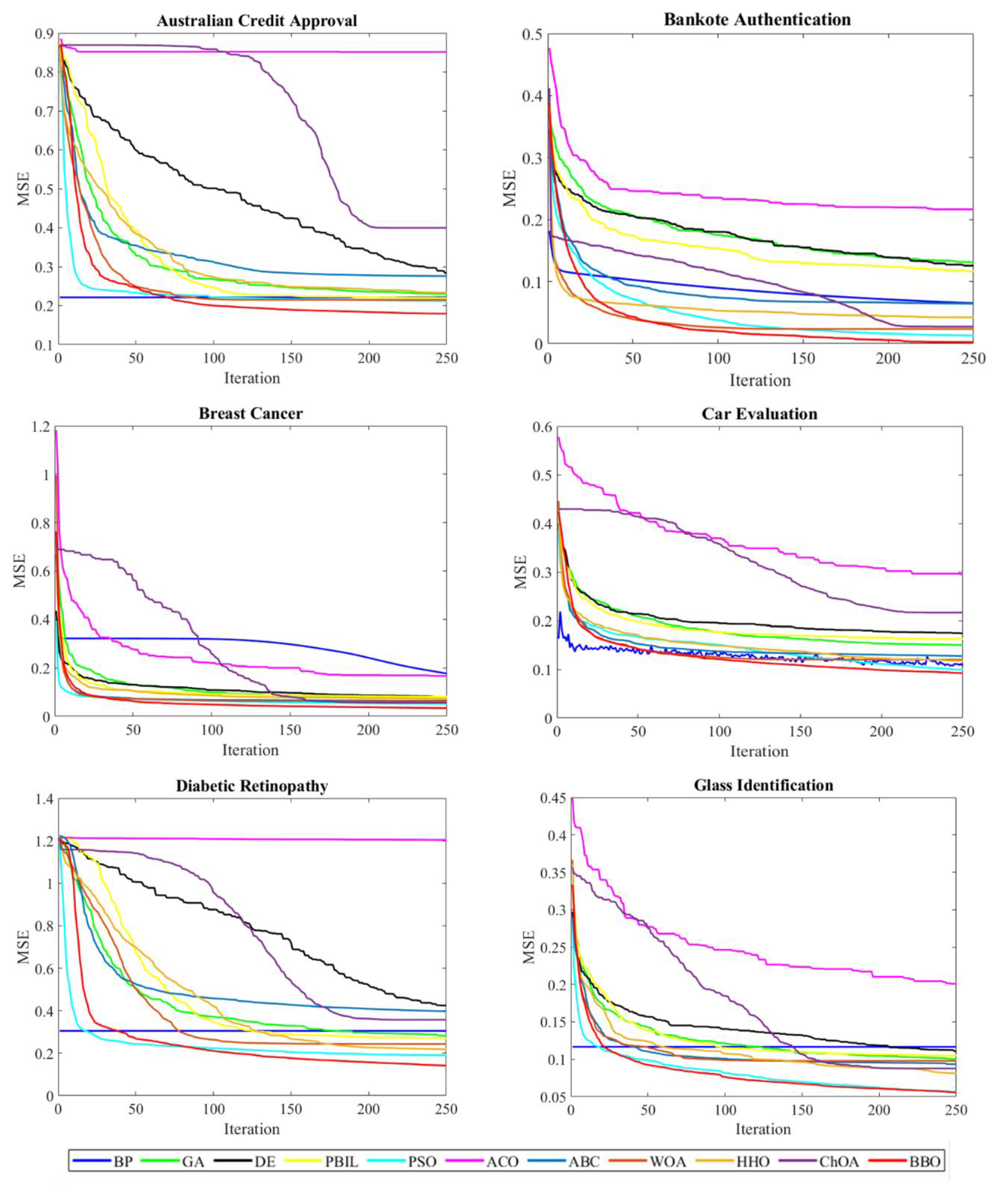
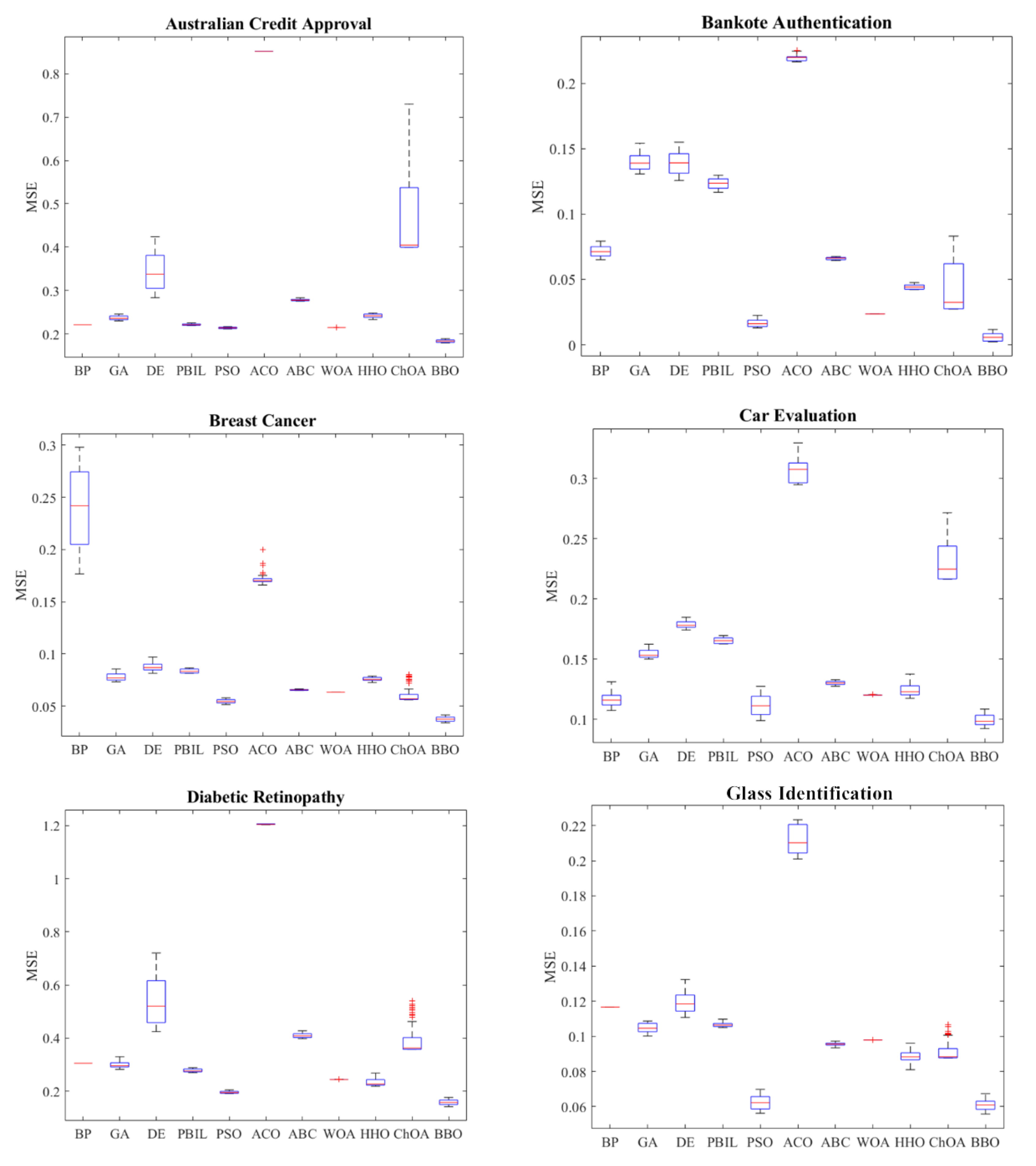
• Through the comparison of scientific experiments, the effective intelligent learning algorithm of dendritic neural model for classification problems is determined. By comparing different types of intelligent optimization algorithms, the result shows that the biogeographic optimization algorithm has excellent performance, can quickly obtain high-quality solutions and has excellent convergence speed.

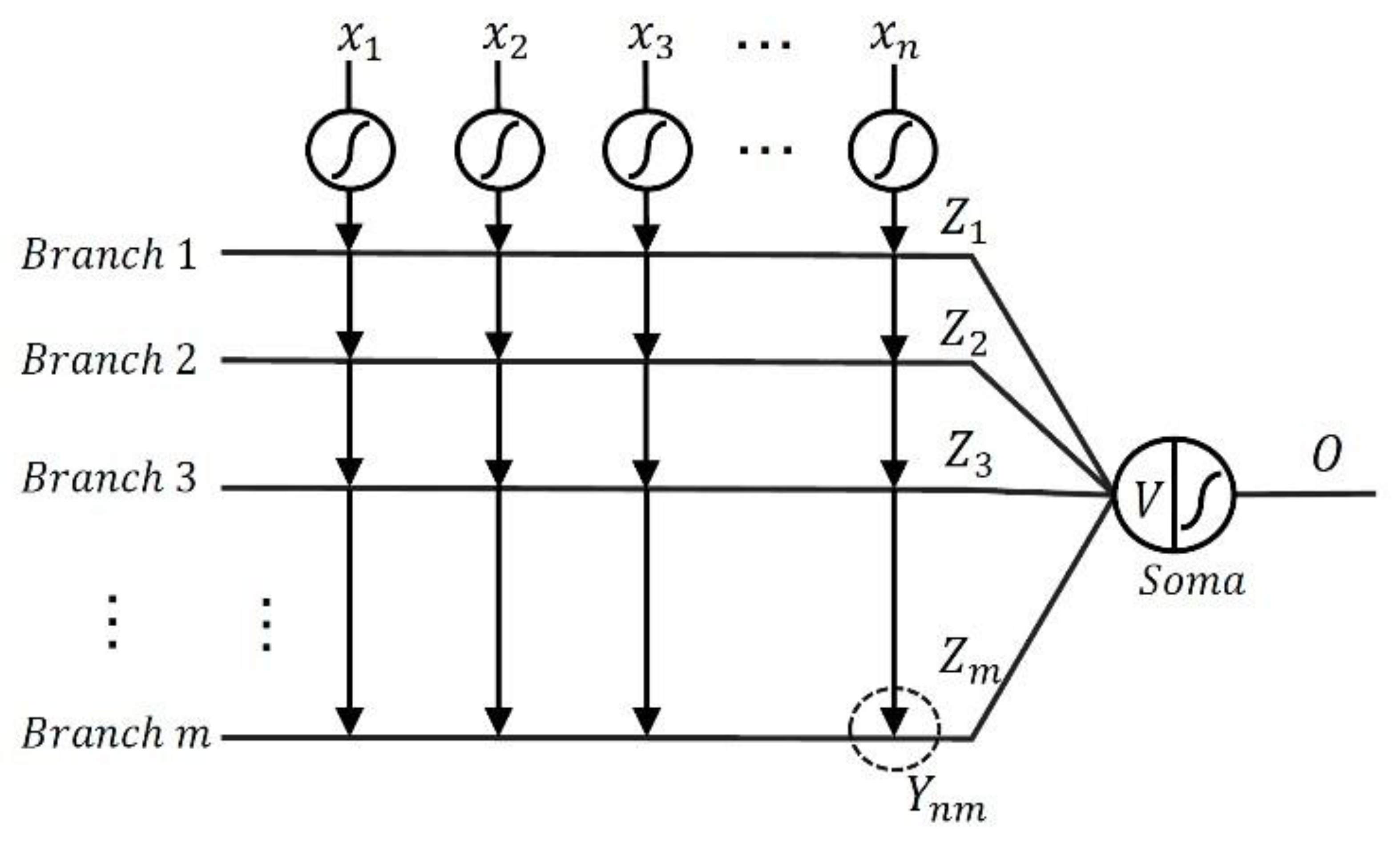
2. Dendritic Neural Model

There exists four layers in the dendritic neural model; they are the synaptic layer, dendritic layer, membrane layer and soma layer. Each layer has corresponding functions and characteristics. The detailed structure of the whole model is shown in Figure 1, where $X=\left\{x_1,x_2,x_3,\dots ,x_n\right\}$ is the input data of model, m branches represent m dendritic layers and O is actual output of model. There are weights and thresholds in each synapse. In the training process of the model, the algorithm will continuously adjust the weights and thresholds in each synapse to optimize the performance of the model. The specific functions of each layer are introduced in detail below.

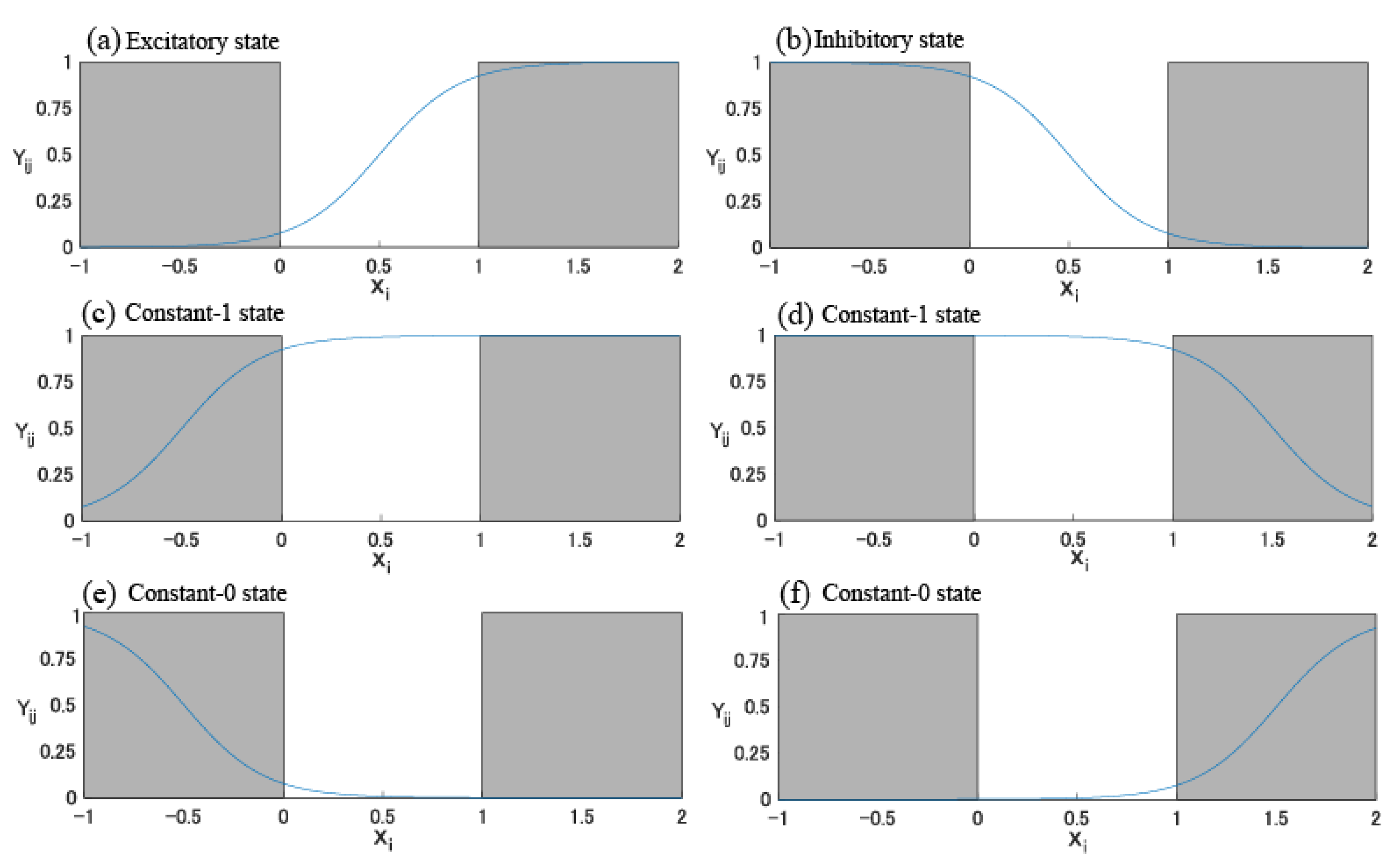
2.1. Synaptic Layer

Input vector $X=\left\{x_1,x_2, x_3,\dots ,x_n\right\}$ inputs data from synapses, and the output of synapse layer is obtained by the activation of the sigmoid function. The nodes in the synaptic layer contain the weights and thresholds of the dendritic neural network. In the training process of the model, the intelligent optimization algorithm needs to optimize all the weights and thresholds in the synaptic layer. The expression of the synaptic layer is (1).

$$Y_{ij}=\frac{1}{e^{-k\left({\omega }_{ij}{x}_i-{\theta }_{ij}\right)}}$$

(1)

where k is a user-defined constant. ${\omega }_{ij}$ and ${\theta }_{ij}$ are the corresponding weight and threshold. According to different values of ${\omega }_{ij}$ and ${\theta }_{ij}$, there are six situations: ➀ 0 < ${\theta }_{ij}$ < ${\omega }_{ij}$, ➁ 0 <${\omega }_{ij}$< ${\theta }_{ij}$, ➂ ${\omega }_{ij}$< ${\theta }_{ij}$ < 0, ➃ ${\theta }_{ij}$< ${\omega }_{ij}$< 0, ➄ ${\theta }_{ij}$ < 0 <${\omega }_{ij}$ and ➅ ${\omega }_{ij}$ < 0 <${\theta }_{ij}$_. In case ➀, the output $Y_{ij}$ is proportional to the output $x_i$, which called the Excitatory state; in case ➂, the output $Y_{ij}$ is inversely proportional to the output $x_i$, which is called the Inhibitory state; in cases ➁ and ➅, the value of the output $Y_{ij}$ is always close to 0, which called the Constant-0 state and in cases ➃ and ➄, the value of the output $Y_{ij}$ is always close to 1, which called the Constant-1 state. Figure 2 shows the details of the four states corresponding to the six situations.

2.2. Dendritic Layer

The dendrite layer multiplies results of n synaptic layers. The whole process can be expressed as (2).

$$Z_j={\displaystyle \prod }_{i=1}^n{Y}_{ij}$$

(2)

2.3. Membrane Layer

The membrane layer is connected to m dendritic branches; the function of the membrane is to perform the sum operation over the results of all branches. The whole process can be expressed as (3).

$$V={\displaystyle \sum }_{j=1}^m{Z}_j$$

(3)

2.4. Soma Layer

Finally, the final output of the soma layer is obtained by the sigmoid function, which can be expressed as (4).

$$O=\frac{1}{1+e^{k_{soma}\left(V-{\theta }_{soma}\right)}}$$

(4)

where $k_{soma}$ and ${\theta }_{soma}$ are self-defined parameters.

3. Learning Algorithms

3.1. Backpropagation Algorithm

The traditional dendritic neural model uses the backpropagation algorithm to update weights and thresholds of the model, which adjusts the weight by backpropagation of the training error layer by layer through the chain rule. Firstly, the least squared error between the actual output $O_p$ and the desired output $T_p$ of the target is obtained as follows in (5).

$$E_p=\frac{1}{2}{\left(T_p-O_p\right)}^2$$

(5)

The synaptic parameters ${\omega }_{ij}$ and ${\theta }_{ij}$ are updated along the negative gradient direction; the whole process can be described as (6) and (7).

$$\begin{gathered} \Delta {\omega }_{ij}\left(t\right)={\displaystyle \sum }_{p=1}^P\frac{\partial E_p}{\partial {\omega }_{ij}} \\ \Delta {\theta }_{ij}\left(t\right)={\displaystyle \sum }_{p=1}^P\frac{\partial E_p}{\partial {\theta }_{ij}} \end{gathered}$$

(6)

$$\begin{gathered} {\omega }_{ij}\left(t+1\right)={\omega }_{ij}\left(t\right)-\eta \Delta {\omega }_{ij}\left(t\right) \\ {\theta }_{ij}\left(t+1\right)={\theta }_{ij}\left(t\right)-\eta \Delta {\theta }_{ij}\left(t\right) \end{gathered}$$

(7)

where $\eta$ represents the learning rate; it is usually set to 0.1. According to the structure of the dendritic neural model in Section 2, the whole process of partial differential derivation can be described as (8) and (9).

$$\begin{gathered} \frac{\partial E_p}{\partial {\omega }_{ij}}=\frac{\partial E_p}{\partial O_p}\frac{\partial O_p}{\partial V}\frac{\partial V}{\partial Z_J}\frac{\partial Z_J}{\partial Y_{ij}}\frac{\partial Y_{ij}}{\partial {\omega }_{ij}} \\ \frac{\partial E_p}{\partial {\theta }_{ij}}=\frac{\partial E_p}{\partial O_p}\frac{\partial O_p}{\partial V}\frac{\partial V}{\partial Z_J}\frac{\partial Z_J}{\partial Y_{ij}}\frac{\partial Y_{ij}}{\partial {\theta }_{ij}} \end{gathered}$$

(8)

$$\begin{gathered} \frac{\partial E_p}{\partial O_p}=T_p-O_p \\ \frac{\partial O_p}{\partial V}=\frac{k_s{x}_i{e}^{-k_s\left(V-{\theta }_s\right)}}{{\left(1+e^{-k_s\left(V-{\theta }_s\right)}\right)}^2} \\ \frac{\partial V}{\partial Z_j}=1 \\ \frac{\partial Z_j}{\partial Y_{ij}}={\displaystyle \prod }_{l=1 and l\ne i}^n{Y}_{lj} \\ \frac{\partial Y_{ij}}{\partial {\omega }_{ij}}=\frac{k{x}_i{e}^{-k\left({\omega }_{ij}{x}_i-{\theta }_{ij}\right)}}{{\left(1+e^{-k\left({\omega }_{ij}{x}_i-{\theta }_{ij}\right)}\right)}^2} \\ \frac{\partial Y_{ij}}{\partial {\theta }_{ij}}=\frac{k{e}^{-k\left({\omega }_{ij}{x}_i-{\theta }_{ij}\right)}}{{\left(1+e^{-k\left({\omega }_{ij}{x}_i-{\theta }_{ij}\right)}\right)}^2} \end{gathered}$$

(9)

This paper introduces the intelligent optimization algorithm into the training of the model. Different from the idea of backpropagation algorithm, the intelligent optimization algorithm updates $\omega$ and $\theta$ by iterating to find the optimization individual. Assuming that the input number of the dendritic neural model is n and m is the number of dendritic layers, if a vector represents a viable solution, then $X_i\left(iϵ\left[1,Q\right]\right)$ can be expressed as (10).

$$\begin{gathered} X_i=\left\{x_i^1,x_i^2,\dots ,x_i^n\right\} \\ =\{{\omega }_{11},{\omega }_{12},\dots ,{\omega }_{mn},{\theta }_{11},{\theta }_{12},\dots ,{\theta }_{mn}\} \end{gathered}$$

(10)

where $X_i$ denotes the ith feasible solutions and $\omega$ and $\theta$ are weight and threshold in the dendritic layer. Generally, the intelligent optimization algorithm first initializes a certain number of feasible solutions randomly, and then iteratively optimizes all feasible solutions according to the characteristics of different optimization algorithms until meeting the termination conditions. The optimal solution $X_{best}$ is the optimal solution of the weight and threshold of the dendritic neural model. In the iterative optimization process, the minimum mean squared error (MSE) is used as a loss function to assess the quality of each feasible solution. The minimum mean squared error is calculated by (11).

$$MSE\left(X_i\right)=\frac{1}{2P}{\displaystyle \sum }_{p=1}^P{\left(T_p-O_p\right)}^2$$

(11)

where $T_p$ is desired output of the pth sample, and $O_p$ is the actual output of the pth sample.

3.2. Genetic Algorithm

Referring to the genetic evolution theory of Darwin and Mendel, the genetic algorithm was proposed by J. Holland in 1975 firstly. It was developed by simulating the biological evolution mechanism in nature. The individual of population is called the chromosome. The constant updating of chromosomes during iteration is called heredity. Inheritance consists of three parts—selection, crossover and mutation. Chromosome quality is usually evaluated by fitness function. At the beginning of the genetic algorithm is the generation of random individuals, according to a predetermined loss function to evaluate each individual, and giving a fitness value. Through the fitness function, the selected individuals produce the next generation. This operation inherits the idea of survival of the fittest in nature, and then the selected individuals combine to produce a new generation through crossover and mutation. The new generation is better than the previous generation because it inherits the excellent characteristics of the previous generation, and the whole population gradually moves towards the optimal solution. According to Algorithm 1, genetic algorithm is mainly divided into the following three parts.

(a)

Selection operator: based on the assessment of individual fitness, selection operator usually selects individuals with higher fitness and eliminates individuals with lower fitness. The common selection methods: fitness allocation method based on proportion or ranking, roulette selection method and so on.

Algorithm 1: Genetic Algorithm.

Begin:   Randomly initialized population of chromosomes $\left(\right\{X_i\}, i\in \left[1,Q\right])$   Evaluate the fitness value for each chromosome using Equation (11)   while Termination criterion     Selection the best chromosome by Roulette Wheel Selection     Generating new chromosomes through single-point crossover and mutation     Evaluate the fitness value of the new chromosome     Replace the population’s worst chromosomes with the greatest new chromosomes     t = t + 1    end while   return the best solution End

(b)

Crossover operator: in the process of biological evolution in nature, two chromosomes form new chromosomes by gene recombination. Therefore, crossover is the core link of the whole process. The design of crossover operator needs to be analyzed for each specific question. The familiar crossover operators such as single point crossover, uniform crossover, multi-point crossover and so on.

(c)

Mutation operator: mutation changes genes inherited on chromosomes by random selection. Mutation itself can be seen as a random algorithm, strictly speaking, an auxiliary algorithm used to generate new individuals.

3.3. Differential Evolution Algorithm

In 1996, Rainer and Kenneth, to solve Chebyshev polynomials, proposed the differential evolution algorithm. The basic idea of DE is to randomly generate a group of the initial population and randomly select three individuals in the initial population; the new individual is generated through summing up the vector difference of two individuals with the third individual according to certain rules. Then, it would compare the new individual with another individual randomly selected in population. If the new individual is superior to the compared individual, it would retain the new individual and eliminate the compared old individual; if the new individual is inferior to the one compared with it, the algorithm would abandon the new individual, retain the old individual compared with it and reselect other individuals from population to generate new individuals. Repeated in this way, the individuals of the initial population are continuously updated until the population reaches a certain optimal state. As shown in Algorithm 2, the process of the differential evolution algorithm includes mutation, crossover and selection operations, which is very similar to the genetic algorithm, but each process has a completely different meaning. It has a variety of mutation strategies. The strategy adopted in the experiment is DE/rand/1, and the formula is shown in (12).

$$V_i=X_{r1}+F·\left(X_{r2}-X_{r3}\right)$$

(12)

Algorithm 2: Differential Evolution Algorithm.

Begin:   F0: Initial mutation operator; CR: Crossover operator   Q: Population; D: Dimension   Initialize the population and calculate the fitness of each population   while Termination criterion     Adaptive mutation operator $\lambda =exp\left(1-\frac{G}{G+1-t}\right), F=F0\ast 2^{\lambda }$     for i = 1: Q      Crossover operator: $V_i=X_{r1}+F·\left(X_{r2}-X_{r3}\right)$      Mutation operator: $u_{ij}=\left\{\begin{array}{c}{v}_{i,j} if rand<CR or randi\left(1,D\right)=j\\ x_{i,j} if rand>CR or randi\left(1,D\right)\ne j\end{array}\right.$      Selection operator: $x_i=\left\{\begin{array}{c}{u}_i if fit\left(u_i\right) superior to fit\left(x_i\right)\\ x_i else \end{array}\right.$     end for     t = t + 1   end while   return the best solution End

3.4. Population-Based Incremental Learning Algorithm

PBIL guides the evolution of the population by maintaining a probability vector. The algorithm selects the individual with the best fitness in each generation to update the probability vector, and the next generation population is generated by the updated probability vector sampling. Repeating these steps, the final optimal solution is obtained. The probability vector is the core part of a population-based incremental learning algorithm. According to Algorithm 3, the main operations related to the probability vector in the algorithm are described below.

Algorithm 3: Population-based Incremental Learning Algorithm.

Begin:   Q: population; LR: learning factor   pm: mutation probability; MS: mutated offset value   Initialization probability vector $P^t, p_i^t=0.5, i=1,2,\dots ,L$     whileTermination criterion     Generate population according to Pt sampling     Evaluate the fitness of each individual according to Equation (11)     Find the individual Bt with the best fitness in the population     Update Pt according to Equations (13) and (14)     t = t + 1   end while   return the best solution End

Assuming that the optimal individual of the current generation is $B^t=\left(b_1^t,b_2^t,\dots ,b_L^t\right)$, the probability vector $P^t$ of the current generation is updated by the following Formula (13).

$$p_i^t=\left(1.0 - LR\right) · p_i^{t-1}+LR·b_i^t, i=1,2,\dots ,L$$

(13)

where LR indicates the learning factor, which is generally set to 0.01. For each $p_i^t$ in the probability vector $P^t$, if random(0, 1) is less than the mutation probability $p_m$, the vector value $p_i^t$ is mutated; otherwise, it is not mutated. Formula is as follows in (14).

$$p_i^{t^{\ast }}=\left(1.0-MS\right) · p_i^t+MS·random\left(0 or 1\right)$$

(14)

where $p_i^{t^{\ast }}$ represents the ith mutated vector value of $P^t$, and MS represents the mutated offset value.

3.5. Particle Swarm Optimization Algorithm

PSO is a stochastic search algorithm developed by simulating the foraging behavior of birds. The algorithm abstracts individual birds into massless, volumetric and informative particles. Since bird populations do not know the specific location of food at first, they can only get the information that food is within a certain range, so bird populations adopt a stable and simple method: search the area around the bird that is closest to the food.

Inspired by this, particle swarm optimization randomly initializes many particles in a solution space, and each particle is given random speed and position information. Then these particles begin to move or stay in place with the initialized speed. After sharing information with the surrounding particles, the approximate orientation of the optimal solution and the position information of the particles closest to the optimal solution is obtained, and the particle moves progressively towards the optimal solution position. The whole process is shown in Algorithm 4. The mathematical formula of particle velocity update mode is described as follows in (15).

$$v_i^t=\omega v_i^{t-1}+c_1{r}_1\left(pbes{t}_i-x_i^{t-1}\right)+c_2{r}_2\left(gbest-x_i^{t-1}\right)$$

(15)

where $c_1$ and $c_2$ are the learning factors of individual extreme and global extreme, $r_1$ and $r_2$ are the influence disturbance factors of individual extreme and global extreme and $pbes{t}_i$ and gbest are the individual extremum and global extreme in the tth iteration.

Algorithm 4: Particle Swarm Optimization Algorithm.

Begin:   Initialize population of particles $\left(\right\{X_i\}, i\in \left[1,Q\right])$   Evaluate fitness for each particle using Equation (11)   Set $pbes{t}_i =X_i, \mathrm{gbest}=\min \left\{\mathrm{pbest}\right\}$   whileTermination criterion     fori = 1: Q     Update the velocity and position of Xi by Equation (15)     Evaluate the fitness of Xi     if fit(Xi) < fit(pbesti)      pbesti = Xi     if fit(pbesti) < fit(gbest)      gbest = pbesti     end for     t = t + 1   end while   return the best solution End

3.6. Ant Colony Optimization Algorithm

ACO was proposed by M. Dorigo firstly, and inspired by real ant colony behavior. The study found that individual ants communicate with each other through a pheromone that allows them to collaborate on complex tasks. Ants tend to move towards the directions with high pheromone concentrations during movement. They not only leave pheromones on the path they pass but also sense the presence and concentration of pheromones during movement to guide their movement direction and search for food. The ant colony algorithm simulates such optimization mechanisms to find the optimal solution through information exchange and cooperation among individuals. The whole simulation process is shown in Algorithm 5. According to the pheromone quantity and heuristic information on each path, the transition probability of the ant at point i at time t to select the next movable point j is (16).

$$P_{ij}^k=\left\{\begin{array}{c}\frac{{\left[{\tau }_{ij}\right]}^{\alpha }·{\left[{\eta }_{ij}\right]}^{\beta }}{{{\displaystyle \sum }}_{s\in allowe{d}_k}{\left[{\tau }_{ij}\right]}^{\alpha }·{\left[{\eta }_{ij}\right]}^{\beta }]}, j\in allowe{d}_k \\ 0, otherwise\end{array}\right.$$

(16)

where $allowe{d}_k=\left\{n-tan{u}_k\right\}$ represents the set of points that ant k at point i is allowed to choose to go next. $\alpha$ represents the influence of pheromone remaining on the path on the subsequent ants’ choice of the path, $\beta$ represents the expected heuristic factor, ${\tau }_{ij}$ is the pheromone concentration and ${\eta }_{ij}$ is the heuristic function.

3.7. Artificial Bee Colony Algorithm

ABC simulates the honey-collecting behavior of honeybees. The location of a nectar source represents the solution, and the pollen quantity of the nectar source represents the value of fitness function. All bees are separated into three groups: the employed bees, the onlooker bees and the explored bees. The number of employed bees is the same as the number of nectar sources, and the number of onlooker bees is half of the number of nectar sources. Firstly, the employed bees take charge of the initial search for nectar sources and collects and shares information. Then the onlooker bees is in charge of staying in the hive and collecting nectar according to the information provided by the employed bees; last, the explored bees are responsible for randomly searching for new nectar sources to replace original ones after original ones are abandoned. According to Algorithm 6, each stage is described as follows.

Algorithm 5: Ant Colony Optimization Algorithm.

Begin:   keep: elitism parameter; ρ: local pheromone decay rate   Q: Population; D: Dimension   Initialize the population and calculate the fitness of each population   whileTermination criterion     fori = 1: Q       for j = 1: Q         Use each solution to update the pheromone for each parameter value: ${\tau }_{ij}=\left(1-\rho \right){\tau }_{ij}+{{\displaystyle \sum }}_{i=1}Q\mathsf{\Delta }{\tau }_{ij}^k$       end for     end for     for k = keep + 1: Q     Use the probability Equation (16) to generate new solutions     end for     t=t+1;   end   return the best solution End

(a)

Employed bees’ stage: employed bees use Formula (17) to find new nectar sources.

$$v_{ij}=x_{ij}+{\phi }_{ij}\left(x_{ij}-x_{kj}\right)$$

(17)

where $x_{kj}$ represents the domain nectar source, and k is not equal to i. ${\rho }_{ij}$ is a random constant between −1 and 1. After obtaining the new nectar source through the above formula, the fitness function values of new and old nectar sources are compared by using the greedy algorithm, and the superior one is selected.

(b)

Onlooker bees’ stage: at this stage, employed bees share nectar information in the dance area. Then onlooker bees analyze information and adopt a roulette strategy to select nectar source tracking mining to ensure that the probability of nectar source mining with higher fitness value is greater.

(c)

Explored bees’ stage: if a nectar source has not been renewed after several mining sessions, the nectar source should be abandoned and the explored bees stage starts. The explored bees use Formula (18) to randomly search for new nectar sources to replace abandoned ones.

$$\begin{array}{c} x_{ij}=x_{minj}+rand\left[0,1\right]\left(x_{maxj}-x_{minj}\right)\end{array}$$

(18)

where $x_{minj}$ and $x_{maxj}$ represent the minimum and maximum values of the jth dimension.

Algorithm 6: Artificial Bee Colony Algorithm.

Begin:   Q: The number of nectar sources or the employed bees;   D: Dimension; O: The number of the onlooker bees   Initialize the nectar sources and calculate the fitness of each nectar source   while Termination criterion     fori = 1: Q      for j = 1: D       Update the location of employed bees by Equation (17)       Store the best nectar sources in a greedy way, and record if not updated      end for     end for     for l = 1: O      Check whether there is nectar source stagnant update. If so, update through Equation (18)     end for     Complete generation update     t = t + 1;   end   return the best solution End

3.8. Whale Optimizaton Algorithm

Mirjalili proposed a WOA-inspired predation mode of humpback whales. Humpback whale individuals can identify and surround prey. According to Algorithm 7, the whole process can be abstracted into three stages: searching prey, surrounding prey and bubble net attack.

(a)

Surrounding prey: humpback whales can recognize prey and continuously reduce their surrounding range. The optimal solution represents target prey or location close to target prey, and other whales will keep approaching it. The entire mathematical model can be interpreted as follows in (19) and (20).

$$\begin{array}{c} D=|C·X^{\ast }\left(t\right)-X\left(t\right)\end{array}$$

(19)

$$X\left(t+1\right)=X^{\ast }\left(t\right)-A·D$$

(20)

where $X^{\ast }\left(t\right)$ is the current optimal whale position vector, t is iterations, $X\left(t\right)$ is the current humpback whale position vector, $A·D$ is bounding step length A and C represent different coefficient vectors.

(b)

Bubble net attack: when a humpback whale surrounds prey, it spits out bubbles in a spiral way to surround the prey. When $\left|A\right|\le 1$, the Formula (21) simulates the spiral hunting behavior of the humpback whale.

$$X_{t+1}=D^{\prime }·e^{bl}·\cos \left(2\pi l\right)+X^{\ast }\left(t\right)$$

(21)

where $D^{\prime }=\left|X^{\ast }\left(t\right)-X\left(t\right)\right|$, $D^{\prime }$ is the distance between current humpback whale position and prey, and b is the constant that determines shape of spiral. l is a random constant in [−1,1].

(c)

Searching prey: when $\left|A\right|>1$, whale individuals are forced to stay away from the optimal whale location of the current generation so that whale individuals randomly search for prey, which is no longer affected by the current optimal whale. Its mathematical model can be described as follows in (22) and (23).

$$D=|C·X_{rand}\left(t\right)-X\left(t\right)$$

(22)

$$X\left(t+1\right)=X_{rand}\left(t\right)-A·D$$

(23)

where $X_{rand}\left(t\right)$ represents the random whale location in the current whale population.

Algorithm 7: Whale Optimization Algorithm.

Begin:   Initialize related parameters, Q: Population   Initialize the population and calculate the fitness of each population   while Termination criterion    fori = 1: Q     if (p < 0.5)       if (|A| < 1)        Update the individual by Equation (19)       else if $(\left|A\right|\ge 1)$       Select a random individual to update by Equation (23)     else if (p ≥ 0.5)       Update the individual by Equation (21)    end for   Calculate individual fitness and update the optimal solution   t = t + 1;   end while   return the best solution End

3.9. Harris Hawks Optimization Algorithm

Inspired by the process of Harris eagle predation, Heidari proposes HHO. The Harris eagle is a group predator, and all are members of the division of labor and coordinated action. The exploration phase is a global search process in which eagles track and detect prey from the air. When the target prey is determined, all members of the group gradually approach the location of the prey, find a suitable position around the prey and complete the encircling for the final attack preparation. The whole simulation process is shown in Algorithm 8. According to the escape behavior of prey and the chase strategy of Harris eagle, Harris Hawks Optimization uses four different strategies to simulate the attack.

(a)

When $\left|E\right|\ge 0.5 \& r\ge 0.5$, in this solution, prey has enough physical strength to try to escape by jumping but is eventually captured; the formula is as follows (24) and (25).

$$X\left(t+1\right)=DX\left(t\right)-E·\left|J·X_{Prey}\left(t\right)-X\left(t\right)\right|$$

(24)

$$DX\left(t\right)=X_{Prey}\left(t\right)-X\left(t\right)$$

(25)

where $DX\left(t\right)$ represents position deviation between eagle group and prey after the tth iteration, and j is the jumping distance during the escape of the prey. $X_{Prey}$ is the position of the prey.

(b)

When $\left|E\right|<0.5 \& r\ge 0.5$, in this solution, prey does not have sufficient energy and is directly captured by the eagle, the formula can be described as follows (26).

$$X\left(t+1\right)=X_{Prey}\left(t\right)-E·\left|DX\left(t\right)\right|$$

(26)

(c)

When $\left|E\right|\ge 0.5 \& r<0.5$, in this solution, the prey has plenty of energy to escape and has the opportunity to escape. Therefore, the eagles form a more intelligent encirclement. The implementation strategies are as follows (27) and (28).

$$Y=X_{Prey}\left(t\right)-E·|J·X_{Prey}\left(t\right)-X\left(t\right)$$

(27)

$$X\left(t+1\right)=\left\{\begin{array}{c}Y, F\left(Y\right)<F\left(X\left(t\right)\right)\\ Z, F\left(Z\right)<F\left(X\left(t\right)\right)\end{array}\right.$$

(28)

Algorithm 8: Harris Hawks Optimization Algorithm.

Begin:   Initialize related parameters, Q: Population   Initialize the population   while Termination criterion    Calculate the fitness of each population    Set Xprey as the best individual    for i = 1: Q     Update the energy E and jump strength J     if$(\left|E\right|\ge 1)$     Update by $X\left(t+1\right)=\left\{\begin{array}{c}{X}_{rand}\left(t\right)-r_1\left|X_{rand}\left(t\right)-2r_{2}X\left(t\right)\right| q\ge 0.5\\ X_{Prey}\left(t\right)-X_m\left(t\right)-r3\left(LB+r_4\left(UB-LB\right)\right) q<0.5\end{array}\right.$     if (|E| < 1)      if (|E| ≥ 0.5 & r ≥ 0.5)       Update by formulae (24) and (25)      else if (|E| < 0.5 & r ≥ 0.5)       Update by Formula (26)      else if (|E| ≥ 0.5 & r < 0.5)       Update by formulae (27) and (28)      else if (|E| < 0.5 & r < 0.5)       Update by formulae (29) and (30)    end for   t = t + 1   end while   return the best solution End

When $\left|E\right|<0.5 \& r<0.5$, in this solution, there is a prey energy shortage but still a chance to escape. Therefore, when the eagles form a hard encirclement to narrow average distance from their prey, the formula can be interpreted as follows in (29) and (30).

$$Y=X_{Prey}\left(t\right)-E·|J·X_{Prey}\left(t\right)-X\left(t\right)$$

(29)

$$X\left(t+1\right)=\left\{\begin{array}{c}Y, F\left(Y\right)<F\left(X\left(t\right)\right)\\ Z, F\left(Z\right)<F\left(X\left(t\right)\right)\end{array}\right.$$

(30)

3.10. Chimp Optimization Algorithm

During chimpanzee hunting, any chimpanzee can randomly change its position in the space around its prey. The mathematical description is as follows in (31) and (32).

$$d=|c{X}_{prey\left(t\right)}-m{X}_{chimp}\left(t\right)$$

(31)

$$X_{chimp}\left(t+1\right)=X_{prey}\left(t\right)-ad$$

(32)

where d is the distance between chimpanzees and prey; t is the current number of iterations; $X_{prey}\left(t\right)$ is the prey position vector; $X_{chimp}\left(t\right)$ is the chimpanzee position vector and a, m, and c are coefficient vectors.

In the chimpanzee community, according to the diversity of intelligence and ability shown by individuals in the process of hunting, chimpanzee groups are classified as “driver”, “barrier”, “chaser” and “attacker”. Each type of chimpanzee has its own ability to think independently and use its own search strategy to explore and predict the location of prey. While they have their own tasks, they also exhibit chaotic individual hunting behavior at the end of the hunt due to social incentives to obtain sexual behavior and benefits. The Chimp Optimization Algorithm solves the problem by simulating the co-hunting behavior of the four chimpanzee species. According to Algorithm 9, the formula for updating the positions of the four chimpanzee groups is described as follows (33)–(35).

$$\left\{\begin{array}{c}{D}_{Attacker}=\left|C_1\ast X_{Attacker}-m\ast X\right|\\ D_{Barrier}=\left|C_2\ast X_{Barrier}-m\ast X\right| \\ D_{Chaser}=\left|C_3\ast X_{Chaser}-m\ast X\right| \\ D_{Driver}=\left|C_4\ast X_{Driver}-m\ast X\right| \end{array}\right.$$

(33)

$$\left\{\begin{array}{c} X_1=X_{Attacker}-A_1\ast D_{Attacker}\\ X_2=X_{Barrier}-A_2\ast D_{Barrier} \\ X_3=X_{Chaser}-A_3\ast D_{Chaser} \\ X_4=X_{Driver}-A_4\ast D_{Driver} \end{array} \right.$$

(34)

$$X\left(t+1\right)=\frac{X_1+X_2+X_3+X_4}{4}$$

(35)

Algorithm 9: Chimp Optimization Algorithm.

Begin:   Initialize f, m, a, and c; Q: Population   Initialize the population and calculate the fitness of each chimp   XAttacker represents the best search agent   XBarrier represents the second best search agent   XChaser represents the third best search agent   XDriver represents the fourth best search agent     while Termination criterion      for i = 1: Q       Update f, m, a and c according to different group strategies       if (μ < 0.5)        if (|a| < 1)         Update the position by (32)        else if (|a| ≥ 1)         Select a search agent randomly       else if (μ ≥ 0.5)         Update the position by $X_{chimp}\left(t+1\right)=\left\{\begin{array}{c}{X}_{prey}\left(t\right)-a.d if \mu <0.5\\ Chaotic\_value if \mu \ge 0.5\end{array}\right.$       end for     Update XAttacker,XBarrier,XChaser,XDriver     t = t + 1     end while   return the best solution End

3.11. Biogeography-Based Optimization Algorithm

BBO is an intelligence algorithm that uses biogeographic theory to solve optimization problems. In a biogeographic optimization algorithm, habitat is used to represent individuals in intelligent optimization algorithm, the suitable index variable (SIV) represents variables in individuals and the habitat suitability index (HSI) represents individual fitness. In nature, the habitat suitability index of each habitat for biological population is different. Habitats with high HSI can accommodate more species and have high species migration rates and low species migration rates. Individual migration can share excellent SIV between habitats. The migration models in biogeography-based optimization mainly include the linear migration model, trapezoidal migration model, secondary migration model and cosine migration model. The linear migration model is used in this paper. Formula (36) is the calculation of immigration rate $\lambda \left(S\right)$; Formula (37) is emigration rate $\mu \left(S\right)$. The entire migration operation is shown in Algorithm 10.

$$\mu \left(S\right)=E\times \frac{S}{S_{max}}$$

(36)

$$\lambda \left(S\right)=I\times \left(1-\frac{S}{S_{max}}\right)$$

(37)

where E represents the probability of maximum emigration, I represents the maximum immigration probability.

Mutation operation simulates the phenomenon that diseases, natural disasters and other factors change the living environment of habitat and lead to the deviation of habitat population from the equilibrium point. According to Algorithm 11, the mutation probability $M_s$ of the species is calculated as follows (38).

$$M_s=M_{max}\times \left(1-\frac{P_s}{P_{Smax}}\right)$$

(38)

where $P_s$ is probability of S species in the habitat; $P_{Smax}$ is the maximum value of $P_s$, and $M_{max}$ represent the maximum mutation rate.

The above introduces how the intelligent optimization algorithm optimizes the weight and threshold of the dendritic neural network. At the same time, the principle, characteristics, important formulas and pseudocode of each algorithm are introduced in detail. Each algorithm has its own characteristics, which also determines the adaptability of the algorithm.

Algorithm 10: Migration Operation(BBO).

Ford = 1: D   if rand() < λi     select another habitat h from the population with the migration probability μj     $H_i\left(d\right)\leftarrow H_j\left(d\right)$   end if End for

Algorithm 11: Mutation Operation(BBO).

Ford = 1: D   if rand() < πi      $H_i\left(d\right)\leftarrow l_d+rand()·\left({\mu }_d-l_d\right)\hspace{1em}\mathrm{end} \mathrm{if}$   end if End for

4. Experiment

For the classification problem of DNM, the experiment compared the results of ten intelligent optimization algorithms and traditional backpropagation algorithms on six classical classification datasets. The software environment of the experiment is MATLAB2018a, and the hardware environment is Intel(R) Core(TM) I5-9500 CPU @ 3.00 GHz, 8.00GB.

All datasets are from the UCI database [54].

Table 1. Details of the dataset.

Classification Datasets	Attributes	Samples	Classes
Australian Credit Approval	15	690	2
Banknote authentication	5	1372	2
Breast cancer	10	699	2
Car Evaluation	7	1728	2
Diabetic Retinopathy	17	520	2
Glass Identification	10	214	2

shows the attributes, number and classes of data in detail. All six data sets are binary classification problems. All datasets are randomly divided into two groups: 70% training and 30% testing. These six datasets contain common classification problems in the real world. For example, the Australian Credit Approval dataset and Banknote Authentication dataset are related to finance, and the Bank Credit Approval dataset concerns credit card applications and is used to evaluate the credit of the new applicant, which can effectively identify the good or bad of the customer, provide the basis for issuing the card and help the bank to establish the first line of defense against credit card risk. The Banknote Authentication dataset is to classify the data extracted from the images of real and counterfeit similar banknote samples. The Breast Cancer dataset and Diabetic Retinopathy dataset are classified datasets about common breast cancer and diabetes. By classifying and predicting different influence attributes of diseases, it has a positive effect on medical treatment activities. The last two dataare on actual production life; the Car Evaluation dataset is a classified data set to assess car safety, and the Glass Identification dataset is a classified data set to classify the type of glass.

To eliminate interference, all experimental results are the average results of 30 independent experiments. The experiment compares the performance of eleven algorithms, including ten intelligent algorithms (GA, DE, PBIL, PSO, ACO, ABC, WOA, HHO, ChOA and BBO) and a traditional back propagation algorithm. The population size of ten intelligent optimization algorithms is 50, and the number of iterations is 250. Other parameters intelligent optimization algorithms of are set according to the experience and characteristics of the algorithm. The initialization parameters of intelligent optimization algorithm are shown in

Table 2. Initialize parameter Settings of intelligent algorithms.

Algorithm	Parameter	Value
GA	Selection mechanism	Roulette wheel
	Crossover probability	0.9
	Mutation probability	0.1
DE	Crossover probability	0.9
	Differential weight	0.5
PBIL	Learning rate	0.05
	Good population member	1
	Bad population member	0
	Elitism parameter	1
	Mutational probability	0.1
PSO	Acceleration constants	[2,2]
	Inertia weights	[0.9,0.5]
ACO	Initial pheromone	1e-6
	Pheromone update constant	20
	Exploration constant	1
	Global pheromone decay rate	0.9
	Local pheromone decay rate	0.5
ABC	Number of employed bee	50
	Number of onlooker bee	25
WOA	Convergence factor a	$a=2-\frac{2·t}{t_{\max }}$
	Coefficient vectors A	$A=2a·rand\left(0,1\right)-a$
HHO	Initial escape energy	inf
ChOA	Initial attacker_score	inf
	Initial barrier_score	inf
	Initial chaser_score	inf
	Initial driver_score	inf
BBO	Habitat modification probability	1
	Mutation probability	0.005
	bound for immigration probability per gene	[0,1]

. The learning rate of the backpropagation algorithm is 0.01, and the number of iterations is 250.

There are four user-defined parameters in DNM, which are the number of synaptic layers M, k of synaptic layer, $k_{soma}$ and ${\theta }_{soma}$ in the activation function of the output layer. The experiment uses Taguchi’s method [55] to obtain a reasonable combination of four parameters of DNM. Taguchi’s method adopts the orthogonal experimental design method, which is a scientific experimental design method to select appropriate and representative points from a large number of experimental points. The four factors of the number of levels are set as follows:$M\in \left\{1,5,10,15,20\right\}$, $k\in \left\{1,5,10,15,25\right\}$, $k_{soma}\in \left\{1,5,10,15,25\right\}$, ${\theta }_{soma}\in \left\{0.1,0.3,0.5,0.7,0.9\right\}$. Full-factor analysis contains $5^4=625$ experiments, orthogonal array ${\mathrm{L}}_{25}\left(5^4\right)$ only contains 25 experiments, it greatly reduces the number of test runs, cost time, manpower, and materials.

Table 3. Optimal parameters of the six datasets in the dendrite neural model.

Classification Datasets	M	k	${\mathit{k}}_{\mathit{s}\mathit{o}\mathit{m}\mathit{a}}$	${\mathit{\theta }}_{\mathit{s}\mathit{o}\mathit{m}\mathit{a}}$
Australian Credit Approval	10	1	10	0.5
Banknote Authentication	10	1	10	0.5
Breast Cancer	10	1	10	0.5
Car Evaluation	20	1	25	0.9
Diabetic Retinopathy	10	1	10	0.5
Glass Identification	10	1	10	0.5

shows the optimal parameters of six datasets obtained through the test of orthogonal array ${\mathrm{L}}_{25}\left(5^4\right)$. The orthogonal matrix experimental results of eleven algorithms in six datasets are recorded in detail in the Appendix A.

In the process of model training optimization, MSE is the loss function of the model, which is the evaluated fitness value of each solution. The accuracy of the classification is to evaluate the performance of the model during the test. Formula (11) is the calculation of MSE, and the calculation method of accuracy is as follows (39).

$$Accuracy=\frac{TP+TN}{TP+FP+TN+FN}\times 100\%$$

(39)

where TP, TN, FP, and FN repent true positives, true negatives, false positives, and false negatives respectively.

5. Result

Figure 3 shows the convergence diagram of the algorithm in the iterative process of optimizing the weights and thresholds of the model, and Figure 4 shows the boxplot of the algorithm after iterative optimization, which can intuitively see the distribution of the optimal solution obtained by the algorithm. At this time, the user-defined parameters of the model adopt the optimal parameters in Table 3.

Table 4. Optimal parameters of the six datasets in the dendrite neural model.

Learning Algorithm	Datasets	M	k	${\mathit{k}}_{\mathit{s}\mathit{o}\mathit{m}\mathit{a}}$	${\mathit{\theta }}_{\mathit{s}\mathit{o}\mathit{m}\mathit{a}}$	Average Accuracy (%) ± Standard Deviation	MSE
BP	Australian Credit Approval	10	1	10	0.5	56.34 ± 2.97	2.21 × 10−1
	Banknote Authentication	10	1	10	0.5	86.50 ± 2.78	6.51 × 10−2
	Breast Cancer	10	1	10	0.5	58.13 ± 25.88	1.77 × 10−1
	Car Evaluation	20	1	25	0.9	75.08 ± 8.89	1.07 × 10−1
	Diabetic Retinopathy	10	1	10	0.5	39.08 ± 2.91	3.05 × 10−1
	Glass Identification	10	1	10	0.5	75.88 ± 4.92	1.17 × 10−1
GA	Australian Credit Approval	10	1	10	0.5	84.21 ± 3.30	2.30 × 10−1
	Banknote Authentication	10	1	10	0.5	91.62 ± 2.45	1.31 × 10−1
	Breast Cancer	10	1	10	0.5	94.98 ± 1.62	7.34 × 10−2
	Car Evaluation	20	1	25	0.9	89.34 ± 1.64	1.50 × 10−1
	Diabetic Retinopathy	10	1	10	0.5	80.66 ± 4.59	2.82 × 10−1
	Glass Identification	10	1	10	0.5	91.98 ± 2.92	1.00 × 10−1
DE	Australian Credit Approval	10	1	10	0.5	82.64 ± 4.09	2.84 × 10−1
	Banknote Authentication	10	1	10	0.5	91.50 ± 2.25	1.26 × 10−1
	Breast Cancer	10	1	10	0.5	94.00 ± 1.33	8.15 × 10−2
	Car Evaluation	20	1	25	0.9	86.63 ± 2.10	1.74 × 10−1
	Diabetic Retinopathy	10	1	10	0.5	69.06 ± 9.17	4.24 × 10−1
	Glass Identification	10	1	10	0.5	92.34 ± 3.61	1.11 × 10−1
PBIL	Australian Credit Approval	10	1	10	0.5	83.11 ± 2.00	2.20 × 10−1
	Banknote Authentication	10	1	10	0.5	92.67 ± 2.00	1.17 × 10−1
	Breast Cancer	10	1	10	0.5	94.35 ± 1.50	8.15 × 10−2
	Car Evaluation	20	1	25	0.9	87.71 ± 1.72	1.63 × 10−1
	Diabetic Retinopathy	10	1	10	0.5	81.54 ± 3.27	2.69 × 10−1
	Glass Identification	10	1	10	0.5	90.26 ± 2.98	1.05 × 10−1
PSO	Australian Credit Approval	10	1	10	0.5	84.34 ± 3.51	2.12 × 10−1
	Banknote Authentication	10	1	10	0.5	98.45 ± 0.89	1.28 × 10−2
	Breast Cancer	10	1	10	0.5	95.06 ± 1.25	5.16 × 10−2
	Car Evaluation	20	1	25	0.9	92.94 ± 2.44	9.89 × 10−2
	Diabetic Retinopathy	10	1	10	0.5	87.16 ± 2.67	1.90 × 10−1
	Glass Identification	10	1	10	0.5	93.00 ± 2.94	5.62 × 10−2
ACO	Australian Credit Approval	10	1	10	0.5	56.10 ± 3.80	8.51 × 10−1
	Banknote Authentication	10	1	10	0.5	88.10 ± 1.31	2.17 × 10−1
	Breast cancer	10	1	10	0.5	90.05 ± 2.75	1.66 × 10−1
	Car evaluation	20	1	25	0.9	82.28 ± 4.68	2.95 × 10−1
	Diabetic retinopathy	10	1	10	0.5	38.70 ± 2.93	1.20 × 100
	Glass Identification	10	1	10	0.5	88.07 ± 3.88	2.01 × 10−1
ABC	Australian Credit Approval	10	1	10	0.5	80.34 ± 6.40	2.76 × 10−1
	Banknote Authentication	10	1	10	0.5	93.23 ± 6.25	6.44 × 10−2
	Breast Cancer	10	1	10	0.5	89.97 ± 15.17	6.50 × 10−2
	Car Evaluation	20	1	25	0.9	87.57 ± 6.31	1.27 × 10−1
	Diabetic Retinopathy	10	1	10	0.5	74.29 ± 10.42	3.97 × 10−1
	Glass Identification	10	1	10	0.5	91.72 ± 3.48	9.34 × 10−2
WOA	Australian Credit Approval	10	1	10	0.5	83.96 ± 3.34	2.15 × 10−1
	Banknote Authentication	10	1	10	0.5	98.67 ± 0.80	2.35 × 10−2
	Breast Cancer	10	1	10	0.5	95.08 ± 1.35	6.33 × 10−2
	Car Evaluation	20	1	25	0.9	91.22 ± 2.57	1.20 × 10−1
	Diabetic Retinopathy	10	1	10	0.5	82.82 ± 6.25	2.43 × 10−1
	Glass Identification	10	1	10	0.5	92.50 ± 2.61	9.79 × 10−2
HHO	Australian Credit Approval	10	1	10	0.5	83.17 ± 5.35	2.34 × 10−1
	Banknote Authentication	10	1	10	0.5	97.53 ± 1.13	4.23 × 10−2
	Breast Cancer	10	1	10	0.5	94.43 ± 2.78	7.27 × 10−2
	Car Evaluation	20	1	25	0.9	91.47 ± 2.14	1.18 × 10−1
	Diabetic Retinopathy	10	1	10	0.5	85.15 ± 5.34	2.18 × 10−1
	Glass Identification	10	1	10	0.5	91.67 ± 3.39	8.10 × 10−2
ChOA	Australian Credit Approval	10	1	10	0.5	71.40 ± 10.97	4.00 × 10−1
	Banknote Authentication	10	1	10	0.5	98.73 ± 0.71	2.73 × 10−2
	Breast Cancer	10	1	10	0.5	95.71 ± 1.39	5.62 × 10−2
	Car Evaluation	20	1	25	0.9	84.43 ± 7.46	2.16 × 10−1
	Diabetic Retinopathy	10	1	10	0.5	69.64 ± 9.35	3.57 × 10−1
	Glass Identification	10	1	10	0.5	93.05 ± 3.53	8.77 × 10−2
BBO	Australian Credit Approval	10	1	10	0.5	84.38 ± 1.91	1.79 × 10−1
	Banknote Authentication	10	1	10	0.5	99.50 ± 0.37	2.28 × 10−3
	Breast Cancer	10	1	10	0.5	95.94 ± 1.15	3.42 × 10−2
	Car Evaluation	20	1	25	0.9	93.32 ± 1.98	9.23 × 10−2
	Diabetic Retinopathy	10	1	10	0.5	89.91 ± 3.19	1.41 × 10−1
	Glass Identification	10	1	10	0.5	93.07 ± 3.30	5.57 × 10−2

summarizes the classification accuracy and minimum mean squared error of each algorithm under the optimized parameters.

As we can see, the BP algorithm converges very slowly in the iterative process. In Australian Credit Approval dataset, Diabetic Retinopathy dataset, and Glass Identification dataset, the algorithm falls into local optimization and loses its function. Its robustness is very poor. ACO and ChOA also have slow convergence speed. In the Australian Credit Approval dataset and Diabetic Retinopathy dataset, it is the same as the BP algorithm, which falls into local traps and has poor overall performance. In the six datasets, BBO has the best convergence effect, followed by PSO. In the first 50 iterations of Australian Credit Approval dataset and Diabetic Retinopathy dataset, the convergence speed of PSO is better than that of BBO, but after 50 iterations, BBO’s convergence value is lower than that of PSO, indicating that BBO has better global search ability than PSO. Unlike the DE algorithm, which has a good effect on some datasets (Breast Cancer, Car Evaluation) and poor effect on some datasets (Australian Credit Approval, Diabetic Retinopathy), BBO has good robustness.

From the distribution of optimal solutions, DNM + BBO still has obvious advantages, with smaller error and stable performance, followed by is DNM + PSO. DNM + ACO and DNM + ChOA have many outliers, which means that the algorithm has poor performance and cannot find a good feasible solution.

As can be seen from Table 4, the classification accuracy of BP in the six datasets is very low, where in the Diabetic Retinopathy dataset it is as low as 39% and the highest at 86.5%. BBO has the highest classification accuracy in all six datasets, reaching 99.5% in the Banknote Authentication dataset. PSO is inferior to BBO. The performance of ACO and ChOA is unstable. For example, in the Diabetic Retinopathy dataset, ACO is as low as 38.7%, and ChOA is as low as 69.6%. Other data sets such as WOA, GA, PBIL and so on have good performance, but the overall performance is worse than BBO. In addition, MSE is the loss function value of the model, and BBO is the smallest in six data sets, which shows that BBO has good performance.

Among the ten intelligent optimization algorithms, DNM + BBO has the fastest convergence speed and the highest accuracy, followed by DNM + PSO. Otherwise DNM + WOA, DNM + GA and so on have good convergence speeds and higher classification, but they are still lower than BBO as a whole. Meanwhile, just like the ideal of “no free lunch”, not all intelligent optimization algorithms are suitable for the classification of dendritic neural models. For example, DNM + ACO and DNM + ChOA have poor performance.

In contrast, intelligent optimization algorithms have obvious advantages, the performance of the intelligent dendrite neural model is far better than that of the traditional dendrite neural model.

6. Conclusions

In this paper, an intelligent dendritic neural model is proposed for the first time, which uses intelligent optimization algorithm instead of the traditional BP algorithm to train the model. In the experiment, ten intelligent optimization algorithms including GA, DE, PBIL, PSO, ACO, ABC, WOA, HHO, ChOA, BBO, and traditional BP algorithm were selected to train and test the model on six datasets (Australian Credit Approval, Banknote Authentication, Breast Cancer, Car Evaluation, Diabetic Retinopathy, Glass Identification). These ten algorithms are representative intelligent algorithms, such as GA, DE and BBO based on evolutionary ideas, PBIL based on mathematical statistics, ABC, ACO, PSO, and WOA based on swarm intelligence, and new algorithms HHO, ChOA. The experiment uses Taguchi’s method to obtain a reasonable combination of four parameters of DNM. The experiments compare and analyze effectiveness, convergence speed, and classification accuracy of the algorithm. The experimental results show that the intelligent dendritic neural model (DNM-BBO) is obviously superior to the traditional dendritic neural model. At the same time, through the comparison of intelligent optimization algorithms, the result shows that BBO algorithm has excellent performance, and its robustness, accuracy and convergence speed are the best. The intelligent dendritic neural model established in this study is a powerful tool for solving classification problems and provides more choices in practical engineering applications.

References

- Novaković, J.D.; Veljović, A. Evaluation of classification models in machine learning. Theory Appl. Math. Comput. Sci. 2017, 7, 39–46. [Google Scholar]
- Awad, W.A.; ELseiofi, S.M. Machine learning methods for spam e-mail classification. IJCSIT 2011, 3, 173–184. [Google Scholar] [CrossRef]
- Ossama, A.H.; Mohamed, A.R. Convolutional Neural Networks for Speech Recognition. IEEE/ACM Trans. 2014, 22, 1533–1545. [Google Scholar]
- Argentiero, P.; Chin, R. An automated approach to the design of decision tree classifiers. IEEE Trans. 1982, PAMI-4, 51–57. [Google Scholar] [CrossRef]
- Rish, I. An empirical study of the naïve Bayes classifier. IJCAI 2001, 3, 41–46. [Google Scholar]
- Cortes, C.; Vapnik, V. Support-vector networks. Mach. Learn. 1995, 20, 273–297. [Google Scholar] [CrossRef]
- Schalkoff, R.J. Artificial Neural Networks; McGraw-Hill: New York, USA, USA, 1997. [Google Scholar]
- Zouhal, L.M.; Denœux, T. An evidence-theoretic k-NN rule with parameter optimization. IEEE Trans. 1998, 28, 263–271. [Google Scholar] [CrossRef]
- Dietterich, T.G. The Handbook of Brain Theory and Neural Networks; The MIT Press: Cambridge, MA, USA, 2002. [Google Scholar]
- McCulloch, W.S.; Pitts, W. A logical calculus of the ideas immanent in nervous activity. Bull. Math. Biol. 1990, 52, 99–115. [Google Scholar] [CrossRef]
- Rosenblatt, F. The Perceptron: A probabilistic model for information storage and organization in the brain. Psychological Rev. 1958, 65, 386. [Google Scholar] [CrossRef] [Green Version]
- Rumelhart, D.E.; Geoffrey, E.H. Learning representations by back-propagating errors. Nature 1986, 323, 533–536. [Google Scholar] [CrossRef]
- Riess, J. Adaptive neural network control of cyclic movements using functional neuromuscular stimulation. IEEE Trans. 2000, 8, 42–52. [Google Scholar] [CrossRef] [PubMed]
- Albawi, S.; Mohammed, T.A.; Al-zawi, S. Understanding of a Convolutional Neural Network; ICET2017: Antalya, Turkey, 2017. [Google Scholar]
- Terrence, L.F. Feedforward Neural Network Methodology; Springer Science & Business Media: Berlin, Germany, 2006. [Google Scholar]
- Gao, S.C.; Zhou, M.C. Dendritic neuron with effective learning algorithms for classification, approximation, and prediction. IEEE Trans. 2019, 30, 601–614. [Google Scholar] [CrossRef]
- Todo, Y.; Tamura, H.; Yamashita, K.; Tang, Z. Unsupervised learnable neuron model with nonlinear interaction on dendrites. Neural Netw. 2014, 60, 96–103. [Google Scholar] [CrossRef] [PubMed]
- Ji, J.K.; Gao, S.C.; Cheng, J. An approximate logic neuron model with a dendritic structure. Neurocomputing 2016, 173, 1775–1783. [Google Scholar] [CrossRef]
- Gardner, M.W.; Dorling, S.R. Artificial neural networks (the multilayer perceptron)—A review of applications in the atmospheric sciences. Atmos. Environ. 1998, 32, 2627–2636. [Google Scholar] [CrossRef]
- Losonczy, A.; Makara, J. Compartmentalized dendritic plasticity and input feature storage in neurons. Nature 2008, 452, 436–441. [Google Scholar] [CrossRef] [PubMed]
- Losonczy, A.; Magee, J. Integrative properties of radial oblique dendrites in hippocampal CA1 pyramidal neurons. Neuron 2006, 50, 291–307. [Google Scholar] [CrossRef] [Green Version]
- Branco, T.; Häusser, M. The single dendritic branch as a fundamental functional unit in the nervous system. Curr. Opin. Neurobiol. 2010, 20, 494–502. [Google Scholar] [CrossRef]
- Yu, Y.; Wang, Y.R.; Gao, S.C.; Tang, Z. Statistical modeling and prediction for tourism economy using dendritic neural network. Comput. Intell. Neurosci. 2017, 2017, 9. [Google Scholar] [CrossRef] [PubMed]
- Tang, Y.J.; Ji, J.K.; Zhu, Y.L.; Gao, S.C.; Tang, Z.; Todo, Y. A differential evolution-oriented pruning neural network model for bankruptcy prediction. Complexity 2019, 2019, 21. [Google Scholar] [CrossRef] [Green Version]
- Sha, Z.J.; Hu, L.; Todo, Y.; Ji, J.K.; Gao, S.C.; Tang, Z. A breast cancer classifier using a neuron model with dendritic nonlinearity. IEICE Trans. Inf. Syst. 2015, 98, 1365–1376. [Google Scholar] [CrossRef] [Green Version]
- Jiang, T.; Gao, S.C.; Wang, D.Z.; Ji, J.K.; Todo, Y.; Tang, Z. A neuron model with synaptic nonlinearities in a dendritic tree for liver disorders. IEEJ Trans. Electr. Electron. Eng. 2017, 12, 105–115. [Google Scholar] [CrossRef]
- Jia, D.B.; Yuka, F. Validation of large-scale classification problem in dendritic neuron model using particle antagonism mechanism. Electronics 2020, 9, 792. [Google Scholar] [CrossRef]
- Gao, S.C.; Zhou, M.C.; Wang, Z. Fully Complex-valued Dendritic Neuron Model. IEEE Trans. Neural Netw. Learn. Syst. 2021. [Google Scholar] [CrossRef] [PubMed]
- Jia, D.B.; Li, C.H. Application and evolution for neural network and signal processing in large-scale systems. Complexity 2021, 2021, 7. [Google Scholar] [CrossRef]
- Luo, X.D.; Wen, X.H.; Zhou, M.C.; Abusorrah, A. Decision-Tree-Initialized Dendritic Neuron Model for Fast and Accurate Data Classification. IEEE Trans. Neural Netw. Learn. Syst. 2021. [Google Scholar] [CrossRef]
- Jia, D.B.; Dai, H.W. EEG processing in Internet of medical things using non-harmonic analysis: Application and evolution for SSVEP responses. IEEE Access 2019, 7, 11318–11327. [Google Scholar] [CrossRef]
- Jia, D.B.; Zheng, S.X. A Dendritic Neuron Model with Nonlinearity Validation on Istanbul Stock and Taiwan Futures Exchange Indexes Prediction; IEEE CCIS: Nanjing, China, 2018. [Google Scholar]
- Xu, W.X.; Li, C.H. Optimizing the Weights and Thresholds in Dendritic Neuron Model Using the Whale Optimization Algorithm; Journal of Physics: Conference Series; IOP Publishing: Beijing, China, 2021. [Google Scholar]
- Hecht-Nielsen, R. Theory of the backpropagation neural network. Neural Netw. Percept. 1992, 65–93. [Google Scholar] [CrossRef]
- Ji, J.K.; Song, S.B.; Tang, Y.J.; Gao, S.C.; Tang, Z.; Todo, Y. Approximate logic neuron model trained by states of matter search algorithm. Knowl.-Based Syst. 2019, 163, 120–130. [Google Scholar] [CrossRef]
- Mirjalili, S. Genetic algorithm. In Evolutionary Algorithms and Neural Networks; Springer: Cham, Switzerland; New York, NY, USA, 2019; pp. 43–55. [Google Scholar]
- Whitley, D. A genetic algorithm tutorial. Stat. Comput. 1994, 4, 65–85. [Google Scholar] [CrossRef]
- Ali, K.; Neda, F. A new optimization method: Dolphin echolocation. Adv. Eng. Softw. 2013, 59, 53–70. [Google Scholar]
- Soto, R.; Crawford, B.; Olivares, R. A reactive population approach on the dolphin echolocation algorithm for solving cell manufacturing systems. Mathematics 2020, 8, 1389. [Google Scholar] [CrossRef]
- Dan, S. Biogeography-based optimization. IEEE Trans. 2008, 12, 702–713. [Google Scholar]
- Zhang, Y.; Gu, X. Biogeography-based optimization algorithm for large-scale multistage batch plant scheduling. Expert Syst. Appl. 2020, 162, 113776. [Google Scholar] [CrossRef]
- Höhfeld, M.; Rudolph, G. Towards a theory of population-based incremental learning. In Proceedings of the IEEE Conference on Evolutionary Computation, Indianapolis, IN, USA, 13–16 April 1997; pp. 1–5. [Google Scholar]
- Li, Y.; Feng, X.; Wang, G. Application of Population Based Incremental Learning Algorithm in Satellite Mission Planning. In Proceedings of the International Conference on Wireless and Satellite Systems, Nanjing, China, 17–18 September 2020; Springer: Cham, Switzerland, 2020. [Google Scholar]
- Eberhart, R.; Kennedy, J. A new optimizer using particle swarm theory. In Proceedings of the MHS’95. Proceedings of the Sixth International Symposium on Micro Machine and Human Science, Nagoya, Japan, 4–6 October 1995; IEEE: Nagoya, Japan, 2002. [Google Scholar]
- Wang, F.; Zhang, H.; Zhou, A. A particle swarm optimization algorithm for mixed-variable optimization problems. Swarm Evol. Comput. 2021, 60, 100808. [Google Scholar] [CrossRef]
- Dorigo, M.; Birattari, M. Ant colony optimization. IEEE Commun. Intell. Mag. 2006, 1, 28–39. [Google Scholar] [CrossRef]
- Paniri, M.; Dowlatshahi, M.B.; Nezamabadi-pour, H. MLACO: A multi-label feature selection algorithm based on ant colony optimization. Knowl.-Based Syst. 2020, 192, 105285. [Google Scholar] [CrossRef]
- Karaboga, D. Artificial bee colony algorithm. Scholarpedia 2010, 5, 6915. [Google Scholar] [CrossRef]
- Wang, H.; Wang, W.; Xiao, S.; Cui, Z.; Xu, M. Improving artificial bee colony algorithm using a new neighborhood selection mechanism. Inf. Sci. 2020, 527, 227–240. [Google Scholar] [CrossRef]
- Mirjalili, S.; Lewis, A. The whale optimization algorithm. Adv. Eng. Softw. 2016, 95, 51–67. [Google Scholar] [CrossRef]
- Jafari-Asl, J.; Seghier, M.E.; Ohadi, S. Efficient method using Whale Optimization Algorithm for reliability-based design optimization of labyrinth spillway. Appl. Soft Comput. 2021, 101, 107036. [Google Scholar] [CrossRef]
- Heidari, A.A.; Mirjalili, S. Harris hawks optimization: Algorithm and applications. Future Gener. Comput. Syst. 2019, 97, 849–872. [Google Scholar] [CrossRef]
- Khishe, M.; Mosavi, M.R. Chimp optimization algorithm. Expert Syst. Appl. 2020, 149, 113338. [Google Scholar] [CrossRef]
- UCI Machine Learning Repository. Available online: https://archive.ics.uci.edu/ml/index.php (accessed on 23 October 2021).
- Jugulum, R.; Taguchi, S. Computer-Based Robust Engineering: Essentials for DFSS; ASQ Quality Press: Milwaukee, WI, USA, 2004. [Google Scholar]