1/3 Order Subharmonic Resonance Control of a Mass-Damper-Spring Model via Cubic-Position Negative-Velocity Feedback

Abstract

A cubic-position negative-velocity (CPNV) feedback controller is proposed in this research in order to suppress the nontrivial oscillations of the $1/3$ order subharmonic resonance of a mass-damper-spring model. Based on the Krylov–Bogoliubov (KB) averaging method, the model’s equation of motion is approximately solved and tested for stability. The nontrivial solutions region is plotted to determine where these solutions occur and try to quench them. The controller parameters can play crucial roles in eliminating such regions, keeping only the trivial solutions, and improving the transient response of the car’s oscillations. Different response curves and relations are included in this study to provide the reader a wide overview of the control process.

1. Introduction

Resonance in a mechanical system is a phenomenon where a harmonic-exciting force is applied to such a system at its natural frequency or near it. This case is called the primary resonance at which the system oscillates with a higher amplitude than applying the force at other frequencies. Other secondary resonance cases can happen when the excitation force oscillates at multiples or fractions of the system’s natural frequency. Particularly, the $1/3$ order subharmonic resonance is our case study where the excitation frequency oscillates nearly at three times the natural frequency of the studied model. Nayfeh [1] studied a single degree of freedom (SDOF) system response including quadratic and cubic nonlinearities where the system was subjected to a subharmonic excitation. He concluded two critical values at which the nontrivial amplitudes could exist depending on the initial conditions considered. Nayfeh [2] combined the effects of primary and superharmonic excitations on a SDOF model. The extracted frequency response equation was the same as in the case of primary resonance only, except a shift appeared in the system’s natural frequency. Mook et al. [3] built their analysis on the initial curvature and mid-surface stretching of some transversally excited structural elements. They focused on the subharmonic and internal resonances where the energy could be channeled from one mode to another one of the studied model. Nayfeh and Asfar [4] studied a bar constrained by a nonlinear spring and analyzed its longitudinal response under a harmonic excitation with primary and secondary resonance cases. Rahman and Burton [5] discussed the third order superharmonic resonance in a hardening nonlinearity Duffing oscillator, and the primary resonance in a softening nonlinearity Duffing oscillator. Rega and Benedettini [6] focused on the $1/2$ and $1/3$ order subharmonic resonance cases in order to study the planar oscillations of an elastic cable. Nayfeh and Bouguerra [7] adopted the multiple scales technique to investigate the nonlinear response of a relief valve loaded statically and dynamically at different primary and secondary resonance cases. Feng and Beard [8] relied on the perturbation analysis in order to study the resonance phenomena in conducting a drop under an alternating electric field force. Vakakis [9] discussed the primary and secondary resonance cases in a 2DOF model including a cubic nonlinearity with the help of multiple scales averaging analysis. Tamura et al. [10] introduced an algorithm for extracting the exact solutions of an asymmetrical Duffing equation in its free vibratory state. Wu and Chien [11] combined applying harmonic balance and multiple scales methods in order to present primary and secondary resonances where the transient and steady-state formulas were given together. Nayfeh and Arafat [12] took into account the inertial and cubic-geometric nonlinearities for analyzing the nonlinear behavior of a cantilever metallic beam subjected to combinational resonance. Sorokin et al. [13] modeled a 2DOF mechanism consisting of three rigid bars to form an inverted T with supporting the ends of the horizontal bars on a spring foundation subjected to primary and subharmonic excitations. Allen and Roy [14] studied the nonlinear interactions in linear viscoelastic fluids amongst spherical gas bubbles governed by a system of differential equations based on the linear Maxwell and Jeffreys models. Hamdan et al. [15] focused on extracting the second order approximate solution to a cantilever beam that was vertically mounted and excited harmonically with a principal parametric resonance. El-Bassiouny [16] applied a multi-frequency parametric excitation on a 2DOF model including cubic nonlinearities in order to investigate both subharmonic and internal resonances. Nayfeh [17] made a comparison between the reconstitution multiple scales and the generalized averaging methods in order to determine higher order approximate solutions of different models at different resonance cases. Dunne [18] obtained the subharmonic response of an SDOF oscillator subjected to a hard periodic excitation with the aid of harmonic balance method with a split-frequency. Perret-Liaudet and Rigaud [19] introduced a superharmonic excitation of order $2$ with an experimental study on a pre-loaded vibro-impact Hertzian contact using a test rig that simulated a double sphere-plane contact. Wang et al. [20] concluded the occurrence of subharmonic resonant response in a maglev system by the flexible guideway deflection when controlled by a delayed acceleration feedback. Tatchim Bemmo et al. [21] concluded that the oscillations amplitude of a continuous FitzHugh–Nagumo model could be increased or decreased when transformed to asymmetrical Van der Pol oscillator and subjected to external and parametric force excitations. Ji [22,23] studied the secondary resonances in a mass-damper-spring model controlled by a unit considering time delay where he took into account the bifurcation behavior caused by the absence and presence of time delay phenomenon. Zhang et al. [24] modified the multiple scales analysis as an alternative to the traditional one in order to setup higher order approximations of a subharmonic-excited Duffing equation including quadratic and cubic nonlinearities. Dolev and Bucher [25] utilized a digital signal processor in order to modulate an oscillator stiffness subjected to a higher resonance frequency. Ilyas et al. [26] studied the dynamics of a clamped-clamped micro-beam that was electrostatically actuated and excited by primary and subharmonic excitation forces. Zhao et al. [27] discussed the thermal effects and secondary resonances of suspended cables governed by geometrically nonlinear models. Kandil [28] presented cubic and quintic nonlinearities in a hinged-hinged Euler–Bernoulli beam in order to show the mathematical couplings among the first three discretized modes of the studied model with the help of Galerkin discretization technique. Cong et al. [29] analyzed theoretically the nonlinear dynamics of a cantilever beam (cable-stayed) subjected to simultaneous resonance cases that would be very useful in many civil structures. Kandil et al. [30] proposed a wide study on the primary resonance of a mass-damper-spring model controlled by an active controller where 2D and 3D plots were given to confirm the control process. Kwarta and Allen [31] built a new technique that used near-resonant vibrations in order to estimate the backbones of the normal modes of the studied dynamical system. This research proposes a cubic-position negative-velocity (CPNV) feedback controller in order to mitigate the nontrivial oscillations of the $1/3$ order subharmonic resonance of a mass-damper-spring model. The equation of motion is derived and solved approximately by the Krylov–Bogoliubov (KB) averaging method. Stability analysis is fulfilled in order to check the stable and unstable behaviors of such model before and after applying the control unit.

2. 1/3 Order Subharmonic Resonance Analysis

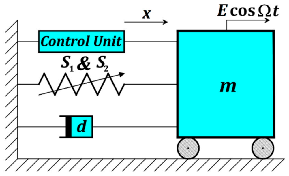
The horizontal displacement $x\left(t\right)$ of the shown car (Figure 1), of mass $m$, is governed by the following ordinary differential equation based on Newton’s law of motion:

$$m\ddot{x}+d\dot{x}+S_{1}x+S_2{x}^3=E\cos \left(\mathsf{\Omega }t\right)+F_c\left(t\right)$$

(1)

where it is attached to a linear dashpot of viscosity factor $d$, a nonlinear spring of linear and cubic stiffness factors $S_1 \& S_2$, and a control unit $F_c\left(t\right)$ which will be discussed next. A harmonic excitation force $E\cos \mathsf{\Omega }t$ affects the car directly leading to severe oscillations that have to be mitigated.

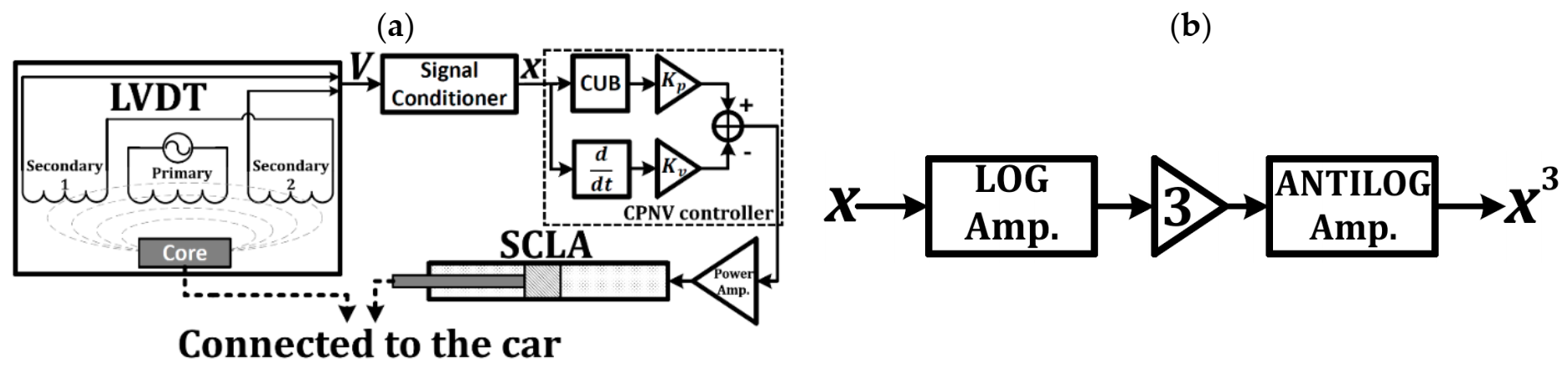
The control unit, shown above, is responsible for acquiring the feedback signal from the car, then creating the suitable actuation force in order to control the car’s oscillation. Figure 2 displays how to achieve such a job starting with getting the feedback signal until applying the control signal. The car’s position is synchronized with the core of the LVDT (linear variable differential transformer) where it produces a voltage signal $V$ proportional with the car’s displacement $x\left(t\right)$. Then, the signal conditioner role becomes relevant and conditions the voltage signal to be like the expected displacement in shape. Next, the $x$ signal is inserted into the CPNV controller in order to generate a control signal in the form $F_c\left(t\right)=K_p{x}^3-K_v\dot{x}$. The control gains $K_p$ and $K_v$ are free adjustable control parameters as shown in Figure 2a. They can be adjusted independently during the online operation for achieving the best results. The cubic signal $x^3$ can be created via a cuber block, as depicted in Figure 2b, which depends on LOG and ANTILOG amplifiers that are explained in any power electronics textbook. The velocity signal $\dot{x}$ can be created via a differentiator block. The generated control signal $F_c\left(t\right)$ can then pass through a power amplifier which provides it with the required power in order to drive the actuator unit in this paper, i.e., the SCLA (servo-controlled linear actuator). This actuator is attached to the car and, in turn, pushes or pulls it to the desired position.

Substituting $F_c\left(t\right)=K_p{x}^3-K_v\dot{x}$ in Equation (1) and simplifying it yields:

$$\ddot{x}+\mu \dot{x}+{\omega }^{2}x+\alpha x^3=f\cos \left(\mathsf{\Omega }t\right)+k_p{x}^3-k_v\dot{x}$$

(2)

where $\mu =d{m}^{-1}$, ${\omega }^2=S_1{m}^{-1}$, $\alpha =S_2{m}^{-1}$, $f=E{m}^{-1}$, $k_p=K_p{m}^{-1}$, and $k_v=K_v{m}^{-1}$. Resorting to the KB averaging method [32], the approximate solution to the nonlinear ordinary differential equation in Equation (2) can be extracted. In this work, the subharmonic secondary resonance is studied and it will not be present unless the forcing amplitude is hard. Hence, we can consider a book-keeping parameter $ϵ$ in order to separate the forced conservative linear problem from the given one. Supposing that $\alpha =ϵ\widehat{\alpha }$, $k_p=ϵ{\widehat{k}}_p$, $k_v=ϵ{\widehat{k}}_v$, and $\mu =ϵ\widehat{\mu }$ in Equation (2) gives us:

$$\ddot{x}+ϵ\widehat{\mu }\dot{x}+{\omega }^{2}x+ϵ\widehat{\alpha }{x}^3=f\cos \left(\mathsf{\Omega }t\right)+ϵ{\widehat{k}}_p{x}^3-ϵ{\widehat{k}}_v\dot{x}$$

(3)

Concerning the forced conservative linear problem ($ϵ=0$), the solution of Equation (3) is:

$$x=a\cos \left(\omega t+\varphi \right)+2\mathsf{\Gamma }\cos \left(\mathsf{\Omega }t\right)$$

(4)

where $a$ and $\varphi$ can be considered time-invariant, while $2\mathsf{\Gamma }=f{\left({\omega }^2-{\mathsf{\Omega }}^2\right)}^{-1}$. Thus:

$$\dot{x}=-\omega a\sin \left(\omega t+\varphi \right)-2\mathsf{\Gamma }\mathsf{\Omega }\sin \left(\mathsf{\Omega }t\right)$$

(5)

Concerning the whole problem ($ϵ\ne 0)$, the solution is still similar to that of Equation (4), but $a$ and $\varphi$ can be considered time-varying. Taking the time-derivative of Equation (4) gives:

$$\dot{x}=\dot{a}\cos \left(\omega t+\varphi \right)-\omega a\sin \left(\omega t+\varphi \right)-a\dot{\varphi }\sin \left(\omega t+\varphi \right)-2\mathsf{\Gamma }\mathsf{\Omega }\sin \left(\mathsf{\Omega }t\right)$$

(6)

Comparing Equations (5) and (6) leads to:

$$\dot{a}\cos \left(\omega t+\varphi \right)-a\dot{\varphi }\sin \left(\omega t+\varphi \right)=0$$

(7)

Taking the time-derivative of Equation (6) gives:

$$\ddot{x}=-\omega \dot{a}\sin \left(\omega t+\varphi \right)-{\omega }^{2}a\cos \left(\omega t+\varphi \right)-\omega a\dot{\varphi }\cos \left(\omega t+\varphi \right)-2{\mathsf{\Gamma }\mathsf{\Omega }}^2\cos \left(\mathsf{\Omega }t\right)$$

(8)

Substituting Equations (4), (5) and (8) into Equation (3) gives us:

$$\dot{a}\sin \left(\omega t+\varphi \right)+a\dot{\varphi }\cos \left(\omega t+\varphi \right)=-ϵ\left(\widehat{\mu }+{\widehat{k}}_v\right)\left(a\sin \left(\omega t+\varphi \right)+\frac{2\mathsf{\Gamma }\mathsf{\Omega }}{\omega }\sin \left(\mathsf{\Omega }t\right)\right)+\frac{ϵ\left(\widehat{\alpha }-{\widehat{k}}_p\right)}{\omega }{\left(a\cos \left(\omega t+\varphi \right)+2\mathsf{\Gamma }\cos \left(\mathsf{\Omega }t\right)\right)}^3$$

(9)

Simultaneous solving of Equations (7) and (9) for $\dot{a}$ and $a\dot{\varphi }$ with reminding that $\alpha =ϵ\widehat{\alpha }$, $k_p=ϵ{\widehat{k}}_p$, $k_v=ϵ{\widehat{k}}_v$, and $\mu =ϵ\widehat{\mu }$ should give us the following:

$$\begin{array}{cc}\hfill \dot{a}& =-\frac{\mu +k_v}{2}a+\frac{\mu +k_v}{2}acos\left(2\omega t+2\varphi \right)-\frac{\mathrm{\Gamma }\mathrm{\Omega }\left(\mu +k_v\right)}{\omega }\left[cos\left(\left(\mathrm{\Omega }-\omega \right)t-\varphi \right)-cos\left(\left(\mathrm{\Omega }+\omega \right)t+\varphi \right)\right]\hfill \\ & +\frac{\alpha -k_p}{\omega }\left[\begin{array}{c}\frac{a^3}{4}sin\left(2\omega t+2\varphi \right)+\frac{a^3}{8}sin\left(4\omega t+4\varphi \right)+{\mathrm{\Gamma }}^{3}sin\left(\left(3\mathrm{\Omega }+\omega \right)t+\varphi \right)-{\mathrm{\Gamma }}^{3}sin\left(\left(3\mathrm{\Omega }-\omega \right)t-\varphi \right)+3{\mathrm{\Gamma }}^{3}sin\left(\left(\mathrm{\Omega }+\omega \right)t+\varphi \right)\hfill \\ -3{\mathrm{\Gamma }}^{3}sin\left(\left(\mathrm{\Omega }-\omega \right)t-\varphi \right)+\frac{3{\mathrm{\Gamma }}^2}{2}asin\left(2\left(\mathrm{\Omega }+\omega \right)t+2\varphi \right)-\frac{3{\mathrm{\Gamma }}^2}{2}asin\left(2\left(\mathrm{\Omega }-\omega \right)t-2\varphi \right)+3{\mathrm{\Gamma }}^{2}asin\left(2\omega t+2\varphi \right)\hfill \\ -\frac{3\mathrm{\Gamma }}{4}{a}^{2}sin\left(\left(\mathrm{\Omega }-\omega \right)t-\varphi \right)+\frac{3\mathrm{\Gamma }}{4}{a}^{2}sin\left(\left(\mathrm{\Omega }+\omega \right)t+\varphi \right)+\frac{3\mathrm{\Gamma }}{4}{a}^{2}sin\left(\left(\mathrm{\Omega }+3\omega \right)t+3\varphi \right)-\frac{3\mathrm{\Gamma }}{4}{a}^{2}sin\left(\left(\mathrm{\Omega }-3\omega \right)t-3\varphi \right)\hfill \end{array}\right]\hfill \end{array}$$

(10a)

$$\begin{array}{cc}\hfill a\dot{\beta }& =-\frac{\mu +k_v}{2}asin\left(2\omega t+2\varphi \right)-\frac{\mathrm{\Gamma }\mathrm{\Omega }\left(\mu +k_v\right)}{\omega }\left[sin\left(\left(\mathrm{\Omega }-\omega \right)t-\varphi \right)+sin\left(\left(\mathrm{\Omega }+\omega \right)t+\varphi \right)\right]\hfill \\ & +\frac{\alpha -k_p}{\omega }\left[\begin{array}{c}\frac{3}{8}{a}^3+\frac{a^3}{2}cos\left(2\omega t+2\varphi \right)+\frac{a^3}{8}cos\left(4\omega t+4\varphi \right)+3{\mathrm{\Gamma }}^{2}a+{\mathrm{\Gamma }}^{3}cos\left(\left(3\mathrm{\Omega }+\omega \right)t+\varphi \right)+{\mathrm{\Gamma }}^{3}cos\left(\left(3\mathrm{\Omega }-\omega \right)t-\varphi \right)\hfill \\ +3{\mathrm{\Gamma }}^{3}cos\left(\left(\mathrm{\Omega }+\omega \right)t+\varphi \right)+3{\mathrm{\Gamma }}^{3}cos\left(\left(\mathrm{\Omega }-\omega \right)t-\varphi \right)+\frac{3{\mathrm{\Gamma }}^2}{2}acos\left(2\left(\mathrm{\Omega }+\omega \right)t+2\varphi \right)+\frac{3{\mathrm{\Gamma }}^2}{2}acos\left(2\left(\mathrm{\Omega }-\omega \right)t-2\varphi \right)\hfill \\ +3{\mathrm{\Gamma }}^{2}acos\left(2\omega t+2\varphi \right)+3{\mathrm{\Gamma }}^{2}acos\left(2\mathrm{\Omega }t\right)+\frac{9\mathrm{\Gamma }}{4}{a}^{2}cos\left(\left(\mathrm{\Omega }-\omega \right)t-\varphi \right)+\frac{9\mathrm{\Gamma }}{4}{a}^{2}cos\left(\left(\mathrm{\Omega }+\omega \right)t+\varphi \right)\hfill \\ +\frac{3\mathrm{\Gamma }}{4}{a}^{2}cos\left(\left(\mathrm{\Omega }+3\omega \right)t+3\varphi \right)+\frac{3\mathrm{\Gamma }}{4}{a}^{2}cos\left(\left(\mathrm{\Omega }-3\omega \right)t-3\varphi \right)\hfill \end{array}\right]\hfill \end{array}$$

(10b)

In Equation (10a,b), there are some slow terms in variation within the interval $\left[0, \pi {\omega }^{-1}\right]$. These terms can be considered almost constant in order to extract the first order approximate solution. For a $1/3$ order subharmonic resonance case ($\mathsf{\Omega }\approx 3\omega$), Equation (10a,b) will be:

$$\dot{a}=-\frac{\mu +k_v}{2}a-\frac{3\mathsf{\Gamma }\left(\alpha -k_p\right)}{4\omega }{a}^2\sin \left(\left(\mathsf{\Omega }-3\omega \right)t-3\varphi \right)$$

(11a)

$$a\dot{\varphi }=\frac{3{\mathsf{\Gamma }}^2\left(\alpha -k_p\right)}{\omega }a+\frac{3\left(\alpha -k_p\right)}{8\omega }{a}^3+\frac{3\mathsf{\Gamma }\left(\alpha -k_p\right)}{4\omega }{a}^2\cos \left(\left(\mathsf{\Omega }-3\omega \right)t-3\varphi \right)$$

(11b)

In the studied subharmonic resonance, the detuning parameter $\sigma$ between the frequencies can be governed by $\sigma =\mathsf{\Omega }-3\omega$ and be inserted into Equation (11a,b) to have an autonomous system as follows:

$$\dot{a}=-\frac{\mu +k_v}{2}a-\frac{3\mathsf{\Gamma }\left(\alpha -k_p\right)}{4\omega }{a}^2\sin \gamma$$

(12a)

$$a\dot{\gamma }=\sigma a-\frac{9{\mathsf{\Gamma }}^2\left(\alpha -k_p\right)}{\omega }a-\frac{9\left(\alpha -k_p\right)}{8\omega }{a}^3-\frac{9\mathsf{\Gamma }\left(\alpha -k_p\right)}{4\omega }{a}^2\cos \gamma$$

(12b)

where $\gamma =\sigma t-3\varphi$. We need to study the steady-state behavior of the system, or in other words, we need to obtain the fixed points of Equation (12a,b). This can be done by supposing that the fluctuations in both $a$ and $\gamma$ are zero, i.e., $\dot{a}=\dot{\gamma }=0$. This leads to an algebraic system of equations in terms of equilibrium amplitude $a_e$ and phase ${\gamma }_e$:

$$\frac{3\left(\mu +k_v\right)}{2}{a}_e=-\frac{9\mathsf{\Gamma }\left(\alpha -k_p\right)}{4\omega }{a}_e^2\sin {\gamma }_e$$

(13a)

$$-\sigma a_e+\frac{9{\mathsf{\Gamma }}^2\left(\alpha -k_p\right)}{\omega }{a}_e+\frac{9\left(\alpha -k_p\right)}{8\omega }{a}_e^3=-\frac{9\mathsf{\Gamma }\left(\alpha -k_p\right)}{4\omega }{a}_e^2\cos {\gamma }_e$$

(13b)

Eliminating ${\gamma }_e$ from Equation (13a,b) yields that either $a_e=0$ (trivial amplitude) or $a_e\ne 0$ (nontrivial amplitude) which can be found from the relation:

$$\frac{9{\left(\mu +k_v\right)}^2}{4}+{\left(\sigma -\frac{9{\mathsf{\Gamma }}^2\left(\alpha -k_p\right)}{\omega }-\frac{9\left(\alpha -k_p\right)}{8\omega }{a}_e^2\right)}^2=\frac{81{\mathsf{\Gamma }}^2{\left(\alpha -k_p\right)}^2}{16{\omega }^2}{a}_e^2$$

(14)

which is quadratic in $a_e^2$ and can be simplified to:

$$\frac{81{\left(\alpha -k_p\right)}^2}{64{\omega }^2}{a}_e^4+\left[-\frac{9\left(\alpha -k_p\right)}{4\omega }\sigma +\frac{243{\mathsf{\Gamma }}^2{\left(\alpha -k_p\right)}^2}{16{\omega }^2}\right]a_e^2+\frac{9{\left(\mu +k_v\right)}^2}{4}+{\left(\sigma -\frac{9{\mathsf{\Gamma }}^2\left(\alpha -k_p\right)}{\omega }\right)}^2=0$$

(15)

It can have a solution in the form:

$$a_e^2=\chi \pm \sqrt{{\chi }^2-\psi }$$

(16)

where:

$$\chi =\frac{8\omega }{9\left(\alpha -k_p\right)}\sigma -6{\mathsf{\Gamma }}^2\mathrm{and} \psi =\frac{64{\omega }^2}{81{\left(\alpha -k_p\right)}^2}\left[\frac{9{\left(\mu +k_v\right)}^2}{4}+{\left(\sigma -\frac{9{\mathsf{\Gamma }}^2\left(\alpha -k_p\right)}{\omega }\right)}^2\right]$$

We note that $\psi$ is always positive, thus nontrivial amplitudes ($a_e\ne 0$) occur only when:

$$\chi >0\Rightarrow {\mathsf{\Gamma }}^2<\frac{4\omega \sigma }{27\left(\alpha -k_p\right)}$$

(17a)

$${\chi }^2-\psi \ge 0\Rightarrow \frac{{\mathsf{\Gamma }}^2\left(\alpha -k_p\right)}{\omega }\left(\sigma -\frac{63{\mathsf{\Gamma }}^2\left(\alpha -k_p\right)}{8\omega }\right)-\frac{1}{2}{\left(\mu +k_v\right)}^2\ge 0$$

(17b)

In case that $\sigma$ is positive (or negative) in Equation (17a), then $\alpha >k_p$ (or $\alpha <k_p$). It is also clear from Equation (17b) that, for a given $\sigma$, nontrivial solutions exist inside a region whose boundary is given in the $\mathsf{\Gamma }\sigma$-plane by:

$$\frac{63{\mathsf{\Gamma }}^2\left(\alpha -k_p\right)}{4\omega }=\sigma \pm \sqrt{{\sigma }^2-\frac{63{\left(\mu +k_v\right)}^2}{4}}$$

(18)

Once the nontrivial solution exists, it should be tested for stability in order to give the reader an indication of the car’s vibration behavior. The car’s amplitude $a$ and phase $\gamma$ can be divided into two terms each such that:

$$a=a_e+a_f$$

(19a)

$$\gamma =+{\gamma }_f$$

(19b)

where {$a_e$, ${\gamma }_e$} are the equilibrium amplitude and phase satisfying Equation (13a,b), and {$a_f$, ${\gamma }_f$} are small fluctuations imposed on the equilibrium ones. Inserting Equation (19a,b) into Equation (12a,b), whilst preserving only the linear terms in {$a_f$, ${\gamma }_f$}, guides us to the following:

$$\left[\begin{array}{c}{\dot{a}}_f\\ {\dot{\gamma }}_f\end{array}\right]=\left[\begin{array}{cc}-\frac{\mu +k_v}{2}-\frac{3\mathsf{\Gamma }\left(\alpha -k_p\right)}{2\omega }{a}_e\sin {\gamma }_e& -\frac{3\mathsf{\Gamma }\left(\alpha -k_p\right)}{4\omega }{a}_e^2\cos {\gamma }_e\\ -\frac{9\left(\alpha -k_p\right)}{4\omega }{a}_e-\frac{9\mathsf{\Gamma }\left(\alpha -k_p\right)}{4\omega }\cos {\gamma }_e& \frac{9\mathsf{\Gamma }\left(\alpha -k_p\right)}{4\omega }{a}_e\sin {\gamma }_e\end{array}\right]\left[\begin{array}{c}{a}_f\\ {\gamma }_f\end{array}\right]$$

(20)

Depending on Equations (13a,b) and (16), one can compute {$a_e$, ${\gamma }_e$} and substitute them in the coefficient matrix of Equation (20). The real parts of the eigenvalues of such matrix will determine whether the equilibrium {$a_e$, ${\gamma }_e$} is asymptotically stable (in case of negative real parts), or otherwise (in case of non-negative real parts).

3. Discussion on the Subharmonic Resonance Curves

As it has been concluded in Equation (18), there is a boundary surrounding the nontrivial amplitudes ($a_e\ne 0$) of the car’s vibrations. Outside this boundary, the car will exhibit only trivial vibrations amplitudes ($a_e=0$). Hence, we are going to plot the relation in Equation (18) to determine the conditions of producing nontrivial amplitudes. The adopted parameters for this process are $\mu =0.01$ as the damping parameter, $\omega =\sqrt{10}$ as the linear natural frequency, $\alpha =0.8$ as the cubic-nonlinearity parameter, $f=25$ as the forcing amplitude, $\mathsf{\Omega }=3\omega +\sigma$ as the forcing frequency, $k_p=0.8$ as the cubic-position control signal gain, and $k_v=0.01$ as the negative-velocity control signal gain. One or more of the aforementioned parameters might be variated for the analysis purpose. 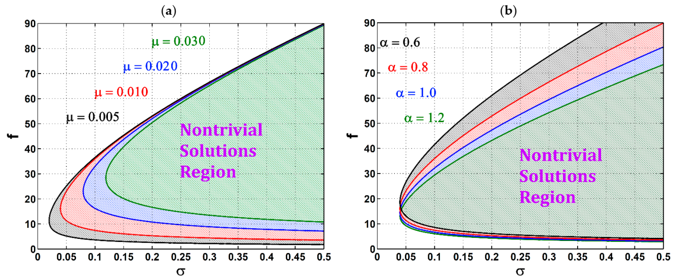Figure 3 depicts the forcing amplitude $f$ versus the forcing frequency detuning $\sigma$ and shows the regions where nontrivial subharmonic solutions exist before control, i.e., $k_p=k_v=0$. In Figure 3a, it is clear that the damping factor $\mu$ is variated to clarify that the bigger $\mu$ is, the smaller the regions become. This gives a clue about the values of $f$ and $\sigma$ that can produce nontrivial amplitudes, while trivial amplitudes can be generated at values other than nontrivial ones. The same is shown in Figure 3b but with various nonlinearity parameter $\alpha$ where $\alpha$ controls the upper and lowers bounds of the region accompanied by a slight shrinking in its size.

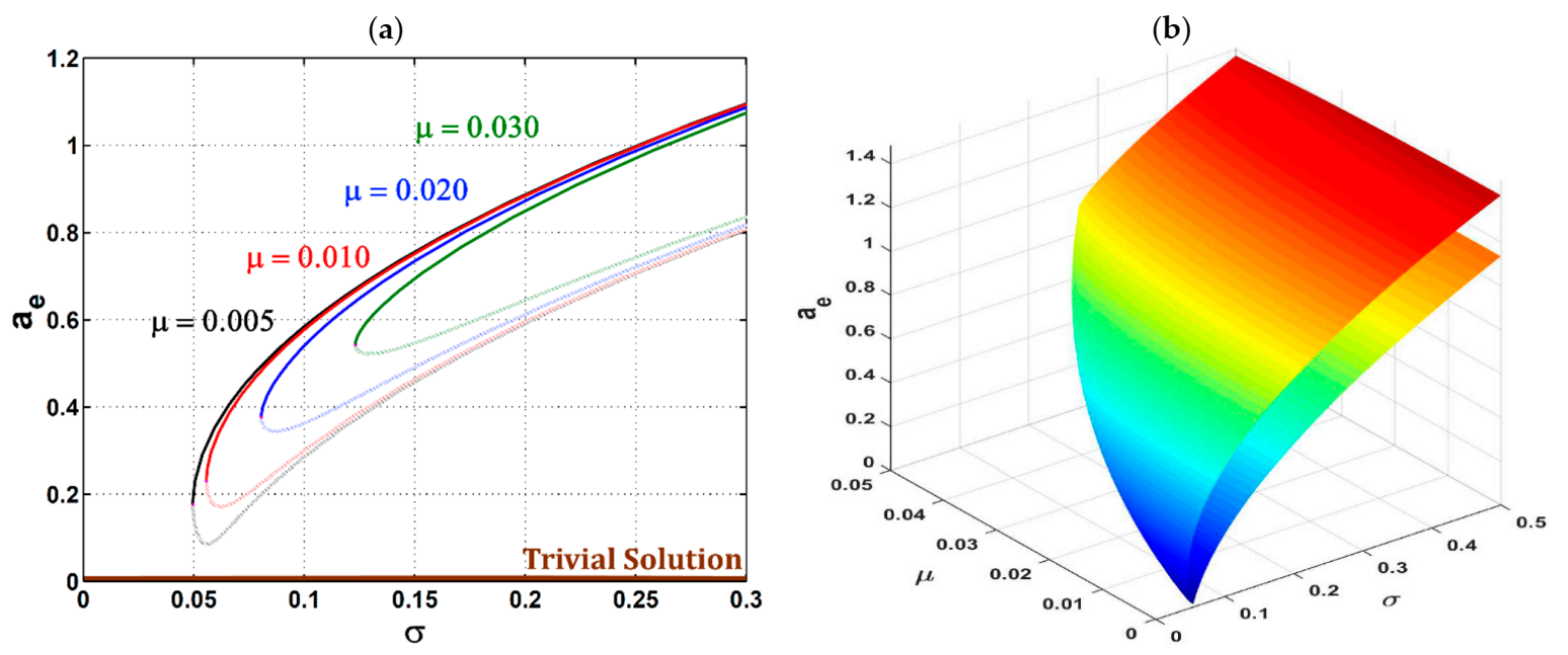
In Figure 4, the equilibrium behavior of the car’s amplitude $a_e$ in terms of the frequency detuning $\sigma$ is plotted for different forcing amplitude $f$ before control ($k_p=k_v=0$). For a better understanding of the behavior, 2D and 3D figures are included. Figure 4a contains solid branches referring to stable amplitude paths, and hatched branches for unstable amplitude paths. These stable and unstable paths meet at Saddle-Node bifurcation points where a real eigenvalue of Equation (20)’s matrix is zero. In this figure, the car exhibits only a trivial amplitude ($a_e=0$) at $\sigma =0$ and greater regardless of the car’s initial displacement. Once $\sigma \in \left[0.040, 0.055\right]$, the car may continue in its trivial behavior or jump to the nontrivial one ($a_e\ne 0$) depending on the car’s initial displacement. The exact value of $\sigma$ where the car can jump to a newer behavior depends on the value of $f$ as shown in the figure. The greater values of $f$ guarantee a bigger vertical distance between the stable and unstable paths as depicted in the figure. Figure 4b showing the 3D plot of the behavior discussed in Figure 4a. It should be noted that the color gradation from red to blue in Figure 4a refers to sweeping from higher amplitude values to lower ones. Figure 5 demonstrates the equilibrium behavior of the car’s amplitude $a_e$ in terms of the frequency detuning $\sigma$ at different damping factor $\mu$ before control ($k_p=k_v=0$). The clear thing in this figure is that increasing the parameter $\mu$ can defer the car’s jump from trivial amplitude to nontrivial one based on the value of $\mu$ and the corresponding value of $\sigma$ where the jump occurs.

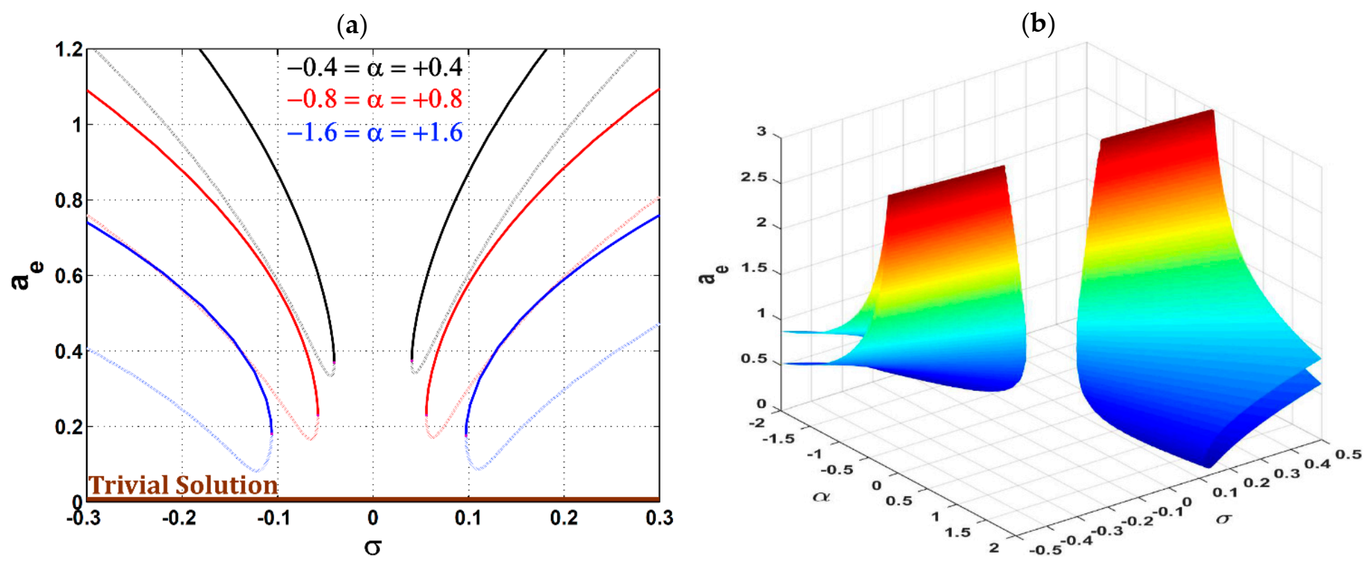
Figure 6 shows the equilibrium behavior of the car’s amplitude $a_e$ in terms of the frequency detuning $\sigma$ at different nonlinearity factor $\alpha$ before control such that $k_p=k_v=0$. According to Equation (17a), $\sigma$ and $\alpha$ (in fact, it is $\left(\alpha -k_p\right)$ but $k_p=0$ in this figure) must have the same sign. Hence, a nonlinear hard spring ($\alpha >0$) will share in producing nontrivial amplitudes for a positive $\sigma$, while a nonlinear soft spring ($\alpha <0$) will share in producing nontrivial amplitudes for a negative $\sigma$ as depicted in the figure. It should also be noted that for $\alpha =0$, there will be no nontrivial amplitudes and the trivial one is the only one which remains as based on Equation (18). Later, this will be a useful feature. Moreover, the nonlinearity value dominates the curve-bending form as seen in both cases of hardening and softening.

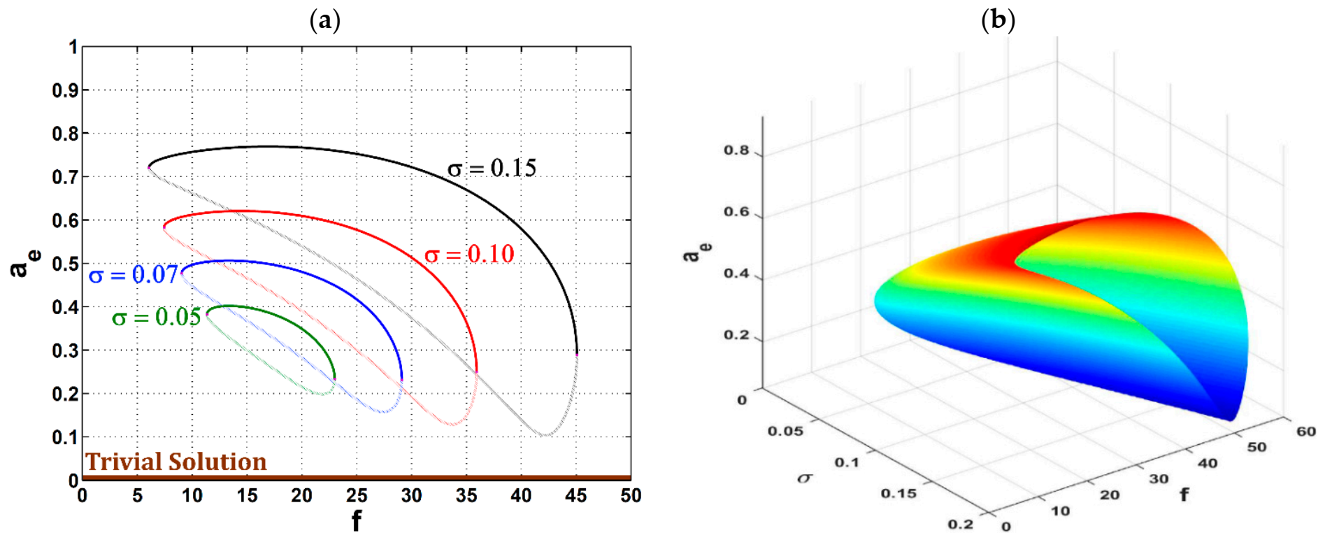
The equilibrium behavior of the car’s amplitude $a_e$ in terms of the forcing amplitude $f$ is shown in Figure 7 at different frequency detuning $\sigma$ before control ($k_p=k_v=0$). It can be noticed that the stable nontrivial amplitudes decrease with increasing force amplitude $f$. Also, the detuning parameter $\sigma$ can raise the level of the nontrivial amplitudes as shown. For smaller $\sigma$, the $f$-range for having trivial amplitudes gets bigger than itself for having both trivial and nontrivial amplitudes. It should be noted that the car can follow either trivial or nontrivial path by changing its initial displacement. 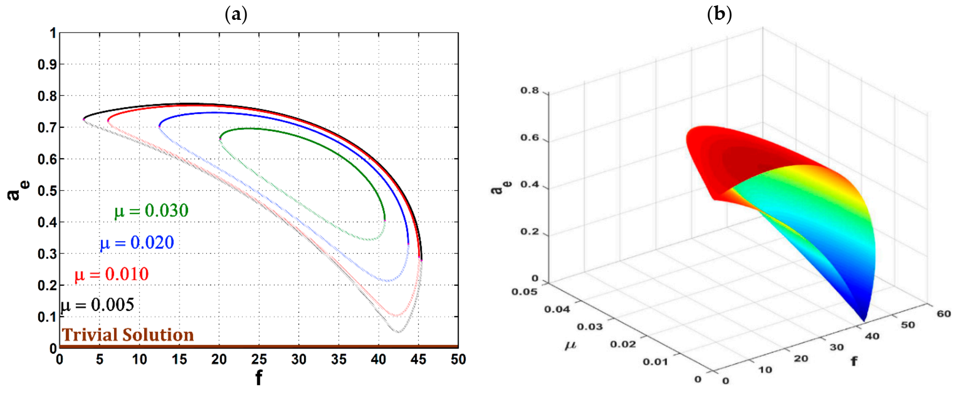In Figure 8, the equilibrium behavior of the car’s amplitude $a_e$ is plotted in terms of the forcing amplitude $f$ at different damping factor $\mu$ before control. 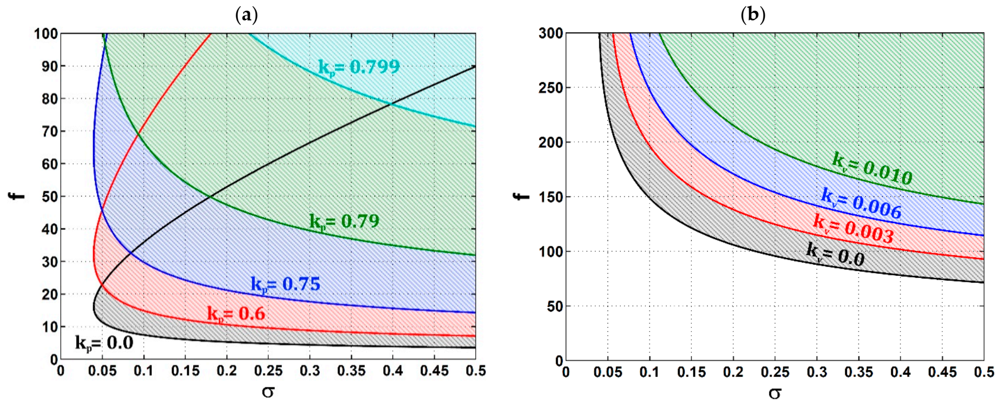This is a reverse approach to Figure 7 where the bigger $\mu$ is, the wider the $f$-range is for having only trivial amplitudes rather than both trivial and nontrivial amplitudes. After control, the relation of the forcing amplitude $f$ versus the forcing frequency detuning $\sigma$ is plotted in Figure 9 to show the retraction of nontrivial solutions region with varying $k_p \& k_v$ and fixing $\alpha \& \mu$. In Figure 9a, the cubic position control gain $k_p$ is variated and the negative-velocity control gain $k_v$ is kept at zero. We can see that the nontrivial solution region shrinks during increasing the parameter $k_p$ until it disappears. As seen from Figure 6 and Equation (18), the existence of nontrivial solution is related to the nonzero value of $\alpha$ before control. After control, this parameter has been modified to $\alpha -k_p$ which provides the foundation of $k_p\to \alpha$ in order to quench the nonlinearity effect and so the nontrivial solutions are as seen in the figure. On the other hand, in Figure 9b, $k_v$ is variated while $k_p$ is kept at $0.799$. It is seen that increasing $k_v$ can help more in quenching the nontrivial solutions region. Moreover, if $k_p$ is kept equal to $\alpha$ (say $0.8$), then there is no need to change $k_v$ as the region has disappeared completely and the trivial solution is the only one existing. 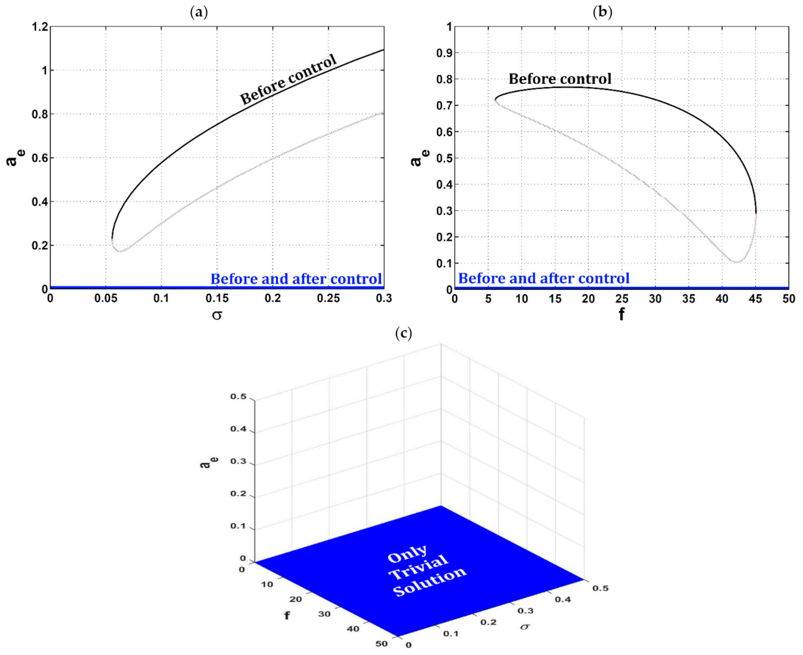The overall target is to eliminate the nontrivial solution ($a_e\ne 0$) and make the system obey the trivial solution only ($a_e=0$) in order to exhibit small oscillations instead of large oscillations. This is clear in Figure 10 showing the controlled equilibrium behavior of the car’s amplitude $a_e$ (at $k_p=0.8$ and $k_v=0.01$) in terms of $\sigma$ (at $f=25$ in Figure 10a), $f$ (at $\sigma =0.15$ in Figure 10b), and both (as a 3D visualization in Figure 10c).

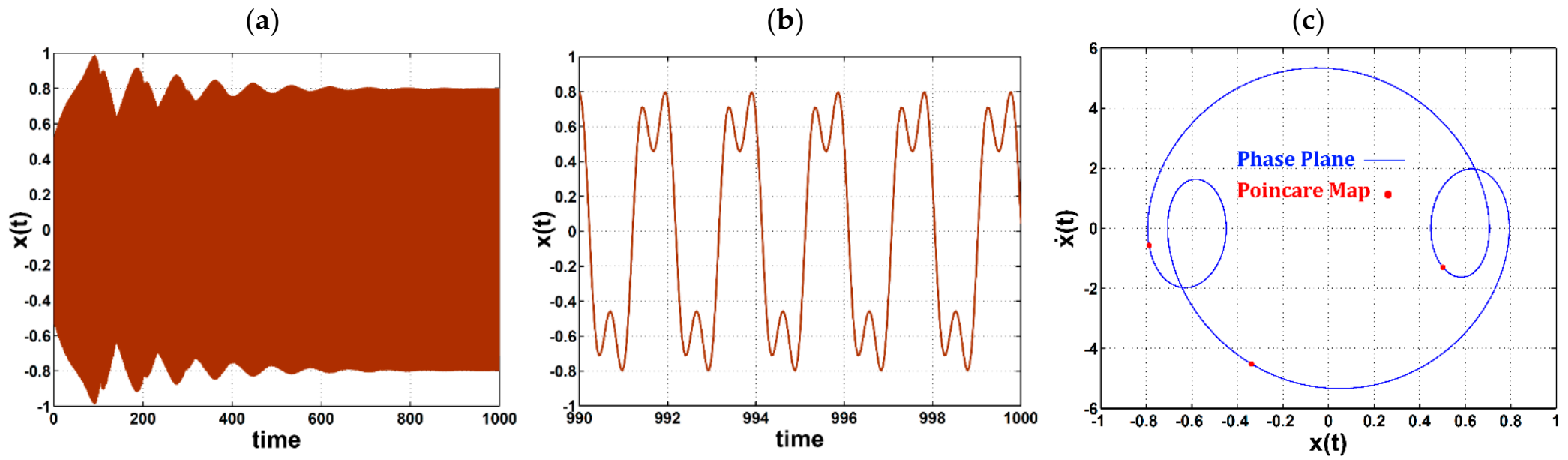
Figure 11, Figure 12, Figure 13 and Figure 14 deal with the simulation of the car’s vibrations before and after control using the fourth order Rung–Kutta numerical technique. Figure 11 presents the car’s nontrivial vibrations in terms of time along with its corresponding phase plane and Poincare map before control at $\sigma =0.15$, $f=25$, $\alpha =0.8$, $\mu =0.01$, and an initial car’s displacement $x\left(0\right)=0.1$. As we have discussed previously, the obedience to either trivial or nontrivial solution depends on the initial condition value. Figure 11a indicates the car’s oscillations amplitude which reaches approximately $80$ cm, while Figure 11b indicates a $10$ s steady-state car’s oscillations to demonstrate the details of the subharmonic solution waveform. Figure 11c portrays the phase plane and Poincare map of the steady-state car’s oscillations where a period-three response can be seen. 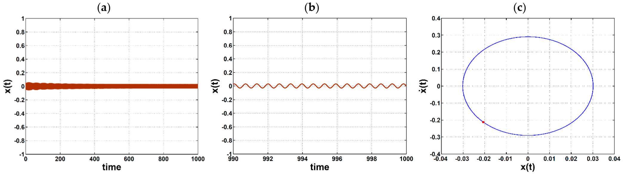Furthermore, Figure 12 shows the car’s trivial vibrations before control at $\sigma =0.15$, $f=25$, $\alpha =0.8$, $\mu =0.01$, and a zero initial car’s displacement $x\left(0\right)=0$. The trivial oscillations amplitude of the car can reach approximately $2$ cm practically (theoretically zero) where a period-one response can be seen. 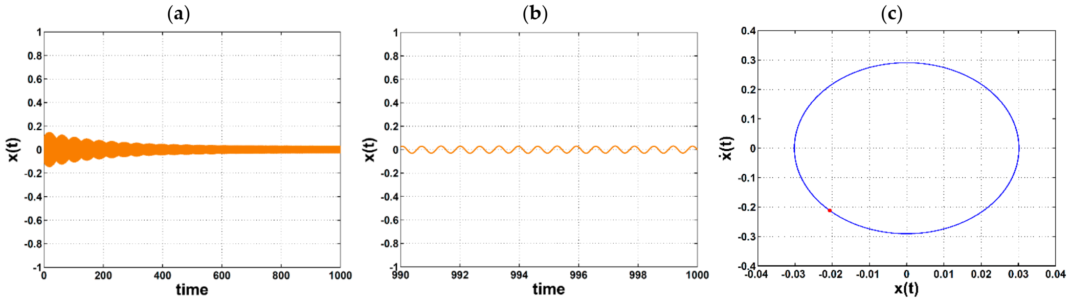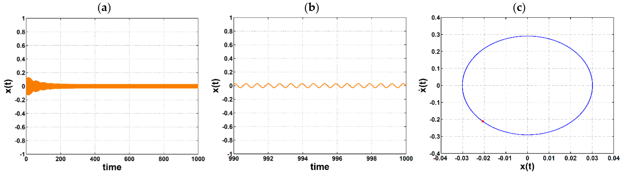Figure 13 shows the car’s vibrations after control at $x\left(0\right)=0.1$, $k_p=0.8$, and $k_v=0$. The nontrivial period-three oscillations have turned into trivial period-one oscillations thanks to the controller, even when the car’s initial displacement is not zero. An important role of the parameter $k_v$ can be seen in Figure 14 where its value changing from $0$ to $0.01$ can enhance the damping behavior of the whole system. Although this does not change the steady-state oscillation amplitude, this shortens the transient-state period and rushes the start of the steady-state period. It is evident in the figure where the steady-state behavior commences at approximately $150$ s, while it commenced at approximately $400$ s in Figure 13 where $k_v=0$.

4. Concluding Remarks

This research proposed a CPNV controller to mitigate the nontrivial oscillations of the $1/3$ order subharmonic resonance of a mass-damper-spring model. The equation of motion has been derived and solved approximately by the KB averaging method. Stability analysis has been fulfilled in order to check the stable and unstable behaviors of such a model before and after applying the control unit. The results of this work can be summarized as follows:

• There was a boundary surrounding the nontrivial amplitudes of the car’s vibrations.
• Outside this boundary, the car would exhibit only trivial vibrations amplitudes.
• The bigger the damping factor $\mu$ was, the smaller the nontrivial solutions regions became.
• The nonlinearity parameter $\alpha$ controlled the upper and lowers bounds of the nontrivial solutions region accompanied by a slight shrinking in its size.
• The car might continue in its trivial behavior or jump to the nontrivial one depending on the car’s initial displacement.
• Increasing the damping factor $\mu$ could defer the car’s jump from trivial amplitude to nontrivial one based on its value and the corresponding value of frequency detuning $\sigma$ where the jump occurred.
• A nonlinear hard spring would share in producing nontrivial amplitudes for a positive detuning $\sigma$, while a nonlinear soft spring would share in producing nontrivial amplitudes for a negative detuning $\sigma$.
• For a linear spring ($\alpha =0$), there would be only trivial amplitudes remaining.
• The stable nontrivial amplitudes decreased with increasing the forcing amplitude $f$.
• The bigger the damping factor $\mu$ was, the wider the forcing amplitude $f$-range was for having only trivial amplitudes rather than both trivial and nontrivial.
• After control, the nontrivial solutions region shrank during increasing the cubic-position control gain $k_p$ till it disappeared.
• Making $k_p$ approach $\alpha$ quenched the nonlinearity effect and so the nontrivial solutions.
• The nontrivial period-three oscillations have turned into trivial period-one oscillations due to the controller, even when the car’s initial displacement is not zero.
• The negative-velocity control gain $k_v$ could enhance the damping behavior of the whole system as it shortened the transient-state period and rushed the start of the steady-state period.

References

1. Nayfeh, A.H. The response of single degree of freedom systems with quadratic and cubic non-linearities to a subharmonic excitation. J. Sound Vib. 1983, 89, 457–470. [Google Scholar] [CrossRef]
2. Nayfeh, A.H. Quenching of primary resonance by a superharmonic resonance. J. Sound Vib. 1984, 92, 363–377. [Google Scholar] [CrossRef]
3. Mook, D.T.; Plaut, R.H.; HaQuang, N. The influence of an internal resonance on non-linear structural vibrations under subharmonic resonance conditions. J. Sound Vib. 1985, 102, 473–492. [Google Scholar] [CrossRef]
4. Nayfeh, A.H.; Asfar, K.R. Response of a bar constrained by a non-linear spring to a harmonic excitation. J. Sound Vib. 1986, 105, 1–15. [Google Scholar] [CrossRef]
5. Rahman, Z.; Burton, T.D. Large amplitude primary and superharmonic resonances in the Duffing oscillator. J. Sound Vib. 1986, 110, 363–380. [Google Scholar] [CrossRef]
6. Rega, G.; Benedettini, F. Planar non-linear oscillations of elastic cables under subharmonic resonance conditions. J. Sound Vib. 1989, 132, 367–381. [Google Scholar] [CrossRef]
7. Nayfeh, A.H.; Bouguerra, H. Non-linear response of a fluid valve. Int. J. Non.-Linear. Mech. 1990, 25, 433–449. [Google Scholar] [CrossRef]
8. Feng, J.Q.; Beard, K.V. Resonances of a conducting drop in an alternating electric field. J. Fluid Mech. 1991, 222, 417–435. [Google Scholar] [CrossRef]
9. Vakakis, A.F. Fundamental and subharmonic resonances in a system with a “1-1” internal resonance. Nonlinear Dyn. 1992, 3, 123–143. [Google Scholar] [CrossRef]
10. Tamura, H.; Okabe, T.; Sueoka, A. Exact Solutions for Free Vibration in an Asymmetrical Duffing Equation. JSME Int. J. Ser. C Dyn. Control Robot. Des. Manuf. 1994, 37, 260–268. [Google Scholar] [CrossRef] [Green Version]
11. Wu, J.J.; Chien, L.C. Solutions to a general forced non-linear oscillations problem. J. Sound Vib. 1995, 185, 247–264. [Google Scholar] [CrossRef]
12. Nayfeh, A.H.; Arafat, H.N. Nonlinear response of cantilever beams to combination and subcombination resonances. Shock Vib. 1998, 5, 277–288. [Google Scholar] [CrossRef] [Green Version]
13. Sorokin, S.V.; Terentiev, A.V.; Karihaloo, B.L. Nonlinear dynamics and stability of a two D.O.F. elastic/elasto-plastic model system. Meccanica 1999, 34, 311–336. [Google Scholar] [CrossRef]
14. Allen, J.S.; Roy, R.A. Dynamics of gas bubbles in viscoelastic fluids. I. Linear viscoelasticity. J. Acoust. Soc. Am. 2000, 107, 3167–3178. [Google Scholar] [CrossRef]
15. Hamdan, M.N.; Al-Qaisia, A.A.; Al-Bedoor, B.O. Comparison of analytical techniques for nonlinear vibrations of a parametrically excited cantilever. Int. J. Mech. Sci. 2001, 43, 1521–1542. [Google Scholar] [CrossRef]
16. El-Bassiouny, A.F. Parametrically excited non-linear systems: A comparison of two methods. Appl. Math. Comput. 2002, 132, 385–410. [Google Scholar] [CrossRef]
17. Nayfeh, A.H. Resolving controversies in the application of the method of multiple scales and the generalized method of averaging. Nonlinear Dyn. 2005, 40, 61–102. [Google Scholar] [CrossRef]
18. Dunne, J.F. Subharmonic-response computation and stability analysis for a nonlinear oscillator using a split-frequency harmonic balance method. J. Comput. Nonlinear Dyn. 2006, 1, 221–229. [Google Scholar] [CrossRef]
19. Perret-Liaudet, J.; Rigaud, E. Superharmonic resonance of order 2 for an impacting Hertzian contact oscillator: Theory and experiments. J. Comput. Nonlinear Dyn. 2007, 2, 190–196. [Google Scholar] [CrossRef]
20. Wang, H.; Li, J.; Zhang, K. Sup-resonant response of a nonautonomous maglev system with delayed acceleration feedback control. IEEE Trans. Magn. 2008, 44, 2338–2350. [Google Scholar] [CrossRef]
21. Tatchim Bemmo, D.; Siewe Siewe, M.; Tchawoua, C. Nonlinear oscillations of the FitzHugh-Nagumo equations under combined external and two-frequency parametric excitations. Phys. Lett. Sect. A Gen. At. Solid State Phys. 2011, 375, 1944–1953. [Google Scholar] [CrossRef]
22. Ji, J.C. Secondary resonances of a quadratic nonlinear oscillator following two-to-one resonant Hopf bifurcations. Nonlinear Dyn. 2014, 78, 2161–2184. [Google Scholar] [CrossRef]
23. Ji, J.C. Two families of super-harmonic resonances in a time-delayed nonlinear oscillator. J. Sound Vib. 2015, 349, 299–314. [Google Scholar] [CrossRef]
24. Zhang, W.; Hu, H.L.; Qian, Y.H.; Gao, F.B. A refined asymptotic perturbation method for nonlinear dynamical systems. Arch. Appl. Mech. 2014, 84, 591–606. [Google Scholar] [CrossRef]
25. Dolev, A.; Bucher, I. Optimizing the dynamical behavior of a dual-frequency parametric amplifier with quadratic and cubic nonlinearities. Nonlinear Dyn. 2018, 92, 1955–1974. [Google Scholar] [CrossRef] [Green Version]
26. Ilyas, S.; Alfosail, F.K.; Bellaredj, M.L.F.; Younis, M.I. On the response of MEMS resonators under generic electrostatic loadings: Experiments and applications. Nonlinear Dyn. 2019, 95, 2263–2274. [Google Scholar] [CrossRef]
27. Zhao, Y.; Huang, C.; Chen, L. Nonlinear planar secondary resonance analyses of suspended cables with thermal effects. J. Therm. Stress. 2019, 42, 1515–1534. [Google Scholar] [CrossRef]
28. Kandil, A. Internal resonances among the first three modes of a hinged–hinged beam with cubic and quintic nonlinearities. Int. J. Non.-Linear. Mech. 2020, 127, 103592. [Google Scholar] [CrossRef]
29. Cong, Y.; Kang, H.; Yan, G. Investigation of dynamic behavior of a cable-stayed cantilever beam under two-frequency excitations. Int. J. Non.-Linear. Mech. 2021, 129, 103670. [Google Scholar] [CrossRef]
30. Kandil, A.; Hamed, Y.S.; Alsharif, A.M.; Awrejcewicz, J. 2D and 3D Visualizations of the Mass-Damper-Spring Model Dynamics Controlled By a Servo-Controlled Linear Actuator. IEEE Access 2021, 9, 153012–153026. [Google Scholar] [CrossRef]
31. Kwarta, M.; Allen, M.S. Nonlinear Normal Mode backbone estimation with near-resonant steady state inputs. Mech. Syst. Signal Process. 2022, 162, 108046. [Google Scholar] [CrossRef]
32. Nayfeh, A.; Mook, D. Nonlinear Oscillations; Wiley: New York, NY, USA, 1995. [Google Scholar]
Figure 1. A controlled car by a control unit with the effect of harmonic force excitation.
Symmetry 14 00685 g001
Figure 2. (a) Control unit design, and (b) implementation of the CUB (cuber) block.
Symmetry 14 00685 g002
Figure 3. f σ -regions where nontrivial subharmonic solutions exist before control ( k p = k v = 0 ): (a) at α = 0.8 and different μ , and (b) at μ = 0.01 and different α .
Symmetry 14 00685 g003
Figure 4. Equilibrium behavior of the car’s amplitude a e in terms of the frequency detuning σ at μ = 0.01 , α = 0.8 , and different forcing amplitude f before control ( k p = k v = 0 ): (a) 2D visualization, and (b) 3D visualization.
Symmetry 14 00685 g004
Figure 5. Equilibrium behavior of the car’s amplitude a e in terms of the frequency detuning σ at f = 25 , α = 0.8 , and different damping factor μ before control ( k p = k v = 0 ): (a) 2D visualization, and (b) 3D visualization.
Symmetry 14 00685 g005
Figure 6. Equilibrium behavior of the car’s amplitude a e in terms of the frequency detuning σ at μ = 0.01 , f = 25 , and different nonlinearity factor α before control ( k p = k v = 0 ): (a) 2D visualization, and (b) 3D visualization.
Symmetry 14 00685 g006
Figure 7. Equilibrium behavior of the car’s amplitude a e in terms of the forcing amplitude f at μ = 0.01 , α = 0.8 , and different frequency detuning σ before control ( k p = k v = 0 ): (a) 2D visualization, and (b) 3D visualization.
Symmetry 14 00685 g007
Figure 8. Equilibrium behavior of the car’s amplitude a e in terms of the forcing amplitude f at σ = 0.15 , α = 0.8 , and different damping factor μ before control ( k p = k v = 0 ): (a) 2D visualization, and (b) 3D visualization.
Symmetry 14 00685 g008
Figure 9. f σ -regions where nontrivial subharmonic solutions exist after control at α = 0.8 , μ = 0.01 and: (a) at k v = 0 and different k p , and (b) at k p = 0.799 and different k v .
Symmetry 14 00685 g009
Figure 10. Controlled equilibrium behavior of the car’s amplitude a e (at k p = 0.8 and k v = 0.01 ) in terms of: (a) σ at f = 25 , (b) f at σ = 0.15 , and (c) σ and f .
Symmetry 14 00685 g010
Figure 11. The car’s nontrivial vibrations in terms of time before control at σ = 0.15 , f = 25 , α = 0.8 , μ = 0.01 , x 0 = 0.1 : (a) overall response, (b) last 10 s of the overall response, and (c) phase plane and Poincare map.
Symmetry 14 00685 g011
Figure 12. The car’s trivial vibrations in terms of time before control at σ = 0.15 , f = 25 , α = 0.8 , μ = 0.01 , x 0 = 0 : (a) overall response, (b) last 10 s of the overall response, and (c) phase plane and Poincare map.
Symmetry 14 00685 g012
Figure 13. The car’s vibrations in terms of time after control ( k p = 0.8 and k v = 0 ) at σ = 0.15 , f = 25 , α = 0.8 , μ = 0.01 , x 0 = 0.1 : (a) overall response, (b) last 10 s of the overall response, and (c) phase plane and Poincare map.
Symmetry 14 00685 g013
Figure 14. The car’s vibrations in terms of time after control ( k p = 0.8 and k v = 0.01 ) at σ = 0.15 , f = 25 , α = 0.8 , μ = 0.01 : (a) overall response, (b) last 10 s of the overall response, and (c) phase plane and Poincare map.
Symmetry 14 00685 g014
Publisher’s Note: MDPI stays neutral with regard to jurisdictional claims in published maps and institutional affiliations.