Article

Transient Controller Design Based on Reinforcement Learning for a Turbofan Engine with Actuator Dynamics

1
School of Energy and Power Engineering, Beihang University, Beijing 100191, China
2
Beihang Hangzhou Innovation Institute Yuhang, Hangzhou 310023, China
3
Research Institute of Aero-Engine, Beihang University, Beijing 100191, China
*
Author to whom correspondence should be addressed.
Symmetry 2022, 14(4), 684; https://doi.org/10.3390/sym14040684
Submission received: 9 March 2022 / Revised: 22 March 2022 / Accepted: 22 March 2022 / Published: 25 March 2022

Abstract

:
To solve the problem of transient control design with uncertainties and degradation in the life cycle, a design method for a turbofan engine’s transient controller based on reinforcement learning is proposed. The method adopts an actor–critic framework and deep deterministic policy gradient (DDPG) algorithm with the ability to train an agent with continuous action policy for the continuous and violent turbofan engine state change. Combined with a symmetrical acceleration and deceleration transient control plan, a reward function with the aim of servo tracking is proposed. Simulations under different conditions were carried out with a controller designed via the proposed method. The simulation results show that during the acceleration process of the engine from idle to an intermediate state, the controlled variables have no overshoot, and the settling time does not exceed 3.8 s. During the deceleration process of the engine from an intermediate state to idle, the corrected speed of high-pressure rotor has no overshoot, the corrected-speed overshoot of the low-pressure rotor does not exceed 1.5%, and the settling time does not exceed 3.3 s. A system with the designed transient controller can maintain the performance when uncertainties and degradation are considered.

1. Introduction

A turbo engine, which is a classical type of aero engine, is a sophisticated piece of thermal equipment with symmetrical geometry. In recent years, with the rapid development of the aerospace industry, the capacity for supersonic and hypersonic flight over a wider flight envelope has been demanded for aero engines [1]. To achieve these goals, more and more complex structures—such as variable cycle, adaptive cycle and turbine-based combined cycle (TBCC) systems—are applied to aero engines, making their modeling and control design more difficult [2]. The control design plays an essential role in the integral aero engine system for a controller, which is responsible for keeping the system asymptotically stable, minimizing the transient process time, and maintaining enough margin to keep the engine working in the event of a surge, extreme temperatures, or excess revolutions.
However, control design is becoming more challenging with modern control theory, making engines so sophisticated that they cannot be modeled accurately. One of the challenges is the existence of disturbances and uncertainties in the aero engine system, which can affect the performance and stability of the system. Therefore, rejection of disturbances and uncertainties has been a critical design objective, which is traditionally achieved by observer and robust control design methods. Observer control is widely used to reject the disturbance [3,4], while robust control can be applied with model uncertainties [5,6,7]. Both observer and robust control design depend on an accurate linear model, where the uncertainties are introduced into the system via linearization. When an accurate linear model is unable to be obtained, these methods design controllers with the idea of sacrificing some performance for robustness. Another challenge is that control parameters should be changed when the components degrade after operating under tough working conditions for a long period of time throughout the whole asymmetrical life cycle [8,9]. When performance degrades, a system with traditional controllers will be vulnerable [10].
Therefore, reinforcement learning is taken into consideration, because it combines the advantages of optimal control and adaptive control [11], meaning that the desired performance can be achieved and the parameters can be adjusted to obtain the required robustness. This is critical because the optimal controller can be obtained without knowing the full system dynamics. As a branch of artificial intelligence, the key to reinforcement learning in feedback control is training the agent with a policy deciding the action of the system. Many algorithms—such as policy iteration, value iteration, Q-learning, deep Q-networks (DQNs), and deep deterministic policy gradient (DDPG)—have been proposed to learn the parameters under different conditions. Policy iteration and value iteration are basic methods of finding optimal values and optimal policy by solving the Bellman equation where policy iteration converges to the optimal value in fewer steps, making value iteration easier to implement [12]. Q-learning methods are based on the Q-function, which is also called the action-value function [13]. The Q-function designs an adaptive control algorithm that converges online to the optimal control solution for complete unknown systems. The DQN is capable of solving problems of high-dimensional observation space, but it cannot be straightforwardly applied to continuous domains, since it relies on finding the action that maximizes the action-value function [14]. The development of DDPG, which is a method of learning continuous action policy, originates from the policy gradient (PG) method developed in 2000 [15]. In 2014, Silver presented deterministic policy gradient (DPG) [16]. More details about the development of DDPG from DPG were given by Lillicrap [13]. Studies using the reinforcement learning method described above have been carried out in the aeronautics and aerospace control industry for learning policies for autonomous planetary landing [17] and unmanned aerial vehicle control [18]. In [19], a deep reinforcement learning technique is applied to a conventional controller for spacecraft. The author of [20] demonstrated that deep reinforcement learning has a possibility to exceed the conventional model-based feedback control in the field of flow control. The DPG algorithm has been adopted to design coupled multivariable controllers for variable cycle engines at set points [21]. The DDPG algorithm has been used to adjust the engine pressure ratio control law online in order to decrease fuel consumption for an adaptive cycle engine [22]. Reinforcement learning is also applied to prediction of aero engines’ gas path health state [23] and life-cycle maintenance [24]. However, few applications of reinforcement learning have been directly used for aero engine control design—especially the transient control design. Turbofan engines take action continuously, with states changing quickly in a wide range of working conditions with uncertainties and degradation. Reinforcement learning is likely to be an ideal way to design the controller for a turbofan engine, since its optimal design procedure is independent of the knowledge of full system dynamics. Therefore, a reinforcement-learning-based controller design method with the agent trained with the DDPG algorithm is proposed in this paper. This is achieved with the turbofan engine nonlinear model, which reduces the uncertainties introduced into the system via linearization. Moreover, this approach has the advantage of designing the set point controller and transient controller together with the same policy, which will restrain the jump from one to the other. A series of improvements are proposed to improve the stability of the closed-loop system, making the training process achievable with a nonlinear model by solving the problem of divergence. Symmetrical performance is achieved in the acceleration and deceleration process of the engine with the designed controller.
The rest of this paper is organized as follows: In Section 2, a nonlinear model of a dual-spool turbofan engine is built and linearized. In Section 3, a brief background of reinforcement learning and DDPG is given. In Section 4, the method of designing the controller for a turbofan engine with reinforcement learning is presented. In Section 5, a series of simulations are applied in different conditions. The simulation results are compared with a traditional gain-scheduled controller, which is designed with linear matrix inequality (LMI) based on an LPV model. Finally, conclusions are given in Section 6.

2. System Uncertainties Analysis

Consider the follow nonlinear system:
{ x ˙ ( t ) = f ( x ( t ) , u ( t ) , d ( t ) ) y ( t ) = g ( x ( t ) , u ( t ) , d ( t ) )
where x ( t ) R x is the state vector of the system, u ( t ) R u is the input vector of the system, y ( t ) R y is the output vector of the system, and d ( t ) R d is the disturbance vector.
Moreover, a linear system is proposed to approximate the dynamic of the nonlinear system for decreasing the nonlinear complexity and making it easier to design the controller k(t), which regulates the y(t) to the desired outputs r(t), based on classic control theory or modern control theory. This can be described as follows:
{ δ x ˙ = A ( x x e ) + B ( u u e ) + G ( d d e ) δ y = C ( x x e ) + D ( u u e ) + H ( d d e )
where xe is the steady-state vector of the system, ue is the input vector that keeps the system working at xe, ye is the steady output vector of the system at state xe with input ue, and de is the disturbance vector at xe. For a stable system, (xe, ue, de), which keeps the system working at steady state, always exists. The nonlinear system at steady state can be described as follows:
{ 0     = f ( x e , u e , d e ) y e = g ( x e , u e , d e )
Matrices of the linear system are usually obtained by linearizing at steady points. A is the state matrix, B is the input matrix, C is the output matrix, D is the feedforward matrix, G is a disturbance matrix, and H is a disturbance matrix. They are obtained as follows:
A = f x | ( x e , u e , d e ) , B = f u | ( x e , u e , d e ) , G = f d | ( x e , u e , d e ) , C = g x | ( x e , u e , d e ) , D = g u | ( x e , u e , d e ) , H = g d | ( x e , u e , d e ) .
As a result, uncertainties are introduced into the system. This is described as follows:
{ ω ( x ˙ ) = f ( x , u , d ) f ( x e , u e , d e ) A ( x x e ) B ( u u e ) G ( d d e ) ω ( y ) = g ( x , u , d ) g ( x e , u e , d e ) C ( x x e ) D ( u u e ) H ( d d e )
The uncertainties depend on the difference between the current state x and the linearized steady state xe. In order to reduce the uncertainties of the linear system when it is used to approximate the nonlinear system over the whole working condition, the linear parameter-varying (LPV) model, which is widely used in modern control theory, is introduced.
For the nonlinear system shown in Equation (1), the LPV model can be obtained by linearizing at n different equilibrium points shown in Equation (3) and scheduling with a parameter. Then, the nonlinear system can be approximated with the LPV model as follows:
{ x ˙ = A ( p ) x + B ( p ) u y = C ( p ) x + D ( p ) u
where p = [ p 1 p 2 p 3 p n ] are the scheduled parameters and j = 1 n p j = 1 , p j 0 . System matrices are defined as follows:
{ A ( p ) = j = 1 n p j A ( j ) B ( p ) = j = 1 n p j B ( j ) C ( p ) = j = 1 n p j C ( j ) D ( p ) = j = 1 n p j D ( j )
where A(j), B(j), C(j), and D(j) are the jth matrices obtained by linearizing the nonlinear system at equilibrium points ( x e ( j ) , u e ( j ) , d e ( j ) ) .
Although the LPV model is proposed with the idea of reducing the uncertainties by reducing the difference between x and xe, the uncertainties introduced into the system in the linearization still exist, and are very hard to calculate.
Moreover, the dynamics and uncertainty of the actuators cannot be ignored in the transient process of an aero engine, and this is usually simplified as a first-order function, which is defined as follows:
u = τ a v τ ˜ a v = [ k 1 τ ˜ a 1 s + 1 0 0 0 k 2 τ ˜ a 2 s + 1 0 0 0 k u τ ˜ a u s + 1 ] v
where u represents the inputs of the engine and v represents the control signals given by the controller. As a result, uncertainties will be introduced into the system again.
The augmented nonlinear system can be described as follows:
{ x ˙ ( t ) = f ( x , v , τ a , d ) y ( t ) = g ( x , v , τ a , d )
The augmented LPV linear model is described as follows:
{ A ( p ) = j = 1 n p j A ( j ) B ( p ) = ( j = 1 n p j B ( j ) ) τ ˜ a C ( p ) = j = 1 n p j C ( j ) D ( p ) = ( j = 1 n p j D ( j ) ) τ ˜ a
Controller design with reinforcement learning is based on the augmented nonlinear model denoted in Equation (8), while controller design with modern control theory relies on the augmented LPV model with uncertainties denoted in Equation (9).

3. Reinforcement Learning Algorithm

3.1. Preliminaries

Definition 1.
The Markov decision process (MDP), which is one of the bases of reinforcement learning, is a memoryless stochastic process denoted with a tuple <S, A, P, R, γ>, where S is a finite set of state, A is the set of action, P is the state transition probability matrix, R is the reward function, and γ is the discounted factor.
Definition 2.
Cumulative reward represents the sum of discounted future reward:
r t γ = i = t γ ( i t ) r ( s i , a i )
where discounted factor γ [ 0 , 1 ] , state s i S , action a i A , and reward function r : S × A .
Theorem 1.
Supposing that the gradient of deterministic policy θ μ θ ( s ) and the gradient of action-value function a Q μ ( s , a ) exist, the parameter θ of the policy is adjusted in the direction of the performance gradient defined as follows:
θ J ( μ θ ) = S ρ μ ( s ) θ μ θ ( s ) a Q μ ( s , a ) | a = μ θ ( s ) d s = E s ~ ρ μ [ θ μ θ ( s ) a Q μ ( s , a ) | a = μ θ ( s ) ]
where μ θ is a deterministic policy with parameter θ , ρ μ is the discounted state distribution with policy μ , Q μ is the action-value function with policy μ , and J is the performance objective s S , a A [15].

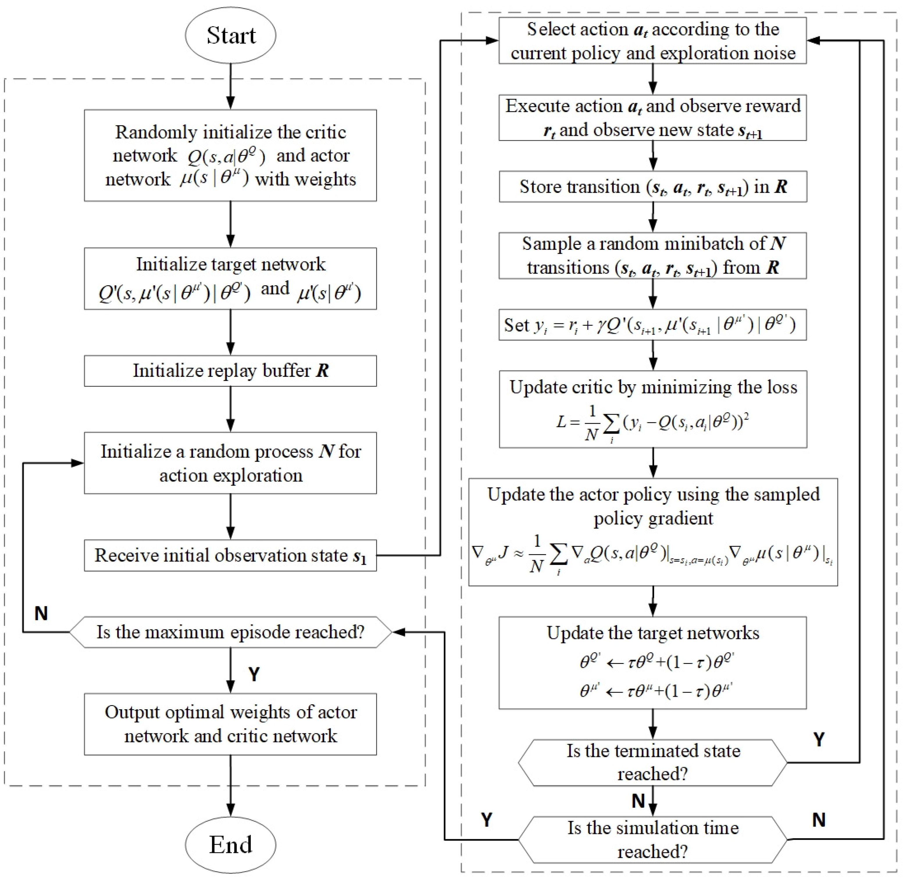
3.2. Framework of Reinforcement Learning

The structure of reinforcement learning consists of an agent and an environment. At time t, the agent observes the state st and reward rt of the environment, and executes action at following the internal policy πθ. Then, the environment outputs the next state st+1 and reward rt+1. This is shown in Figure 1.
The purpose of reinforcement learning is to obtain the agent that contains a policy πθ maximizing the cumulative reward defined in Equation (10) by interacting with the environment. The procedure of training the agent with DDPG is shown in Figure 2.
In this procedure, the DDPG algorithm trains the agent with the actor–critic framework shown in Figure 3. Both critic and actor combine two neural networks: the estimation network, and the target network. The four neural networks are denoted as μ ( s | θ μ ) , Q ( s , a | θ Q ) , μ ( s | θ μ ) , and Q ( s , μ ( s | θ μ ) | θ Q ) , with weights θ μ , θ Q , θ μ , and θ Q , respectively.
(1)
The actor network μ ( s | θ μ ) represents the optimal action policy. It is responsible for iteratively updating the network weights θ μ , choosing the current action ai based on the current state si, and obtaining the next state si+1 and the reward ri;
(2)
The critic network Q ( s , a | θ Q ) represents the Q-value obtained after taking action following the policy defined with the actor network at every state s. It is used to update the network weights θ Q and calculate the current Q ( s i , a i | θ Q ) ;
(3)
The target actor network μ ( s | θ μ ) is a copy of actor network μ ( s | θ μ ) . The weights of the target actor network are updated with the following soft update algorithm:
θ μ τ θ μ + ( 1 τ ) θ μ
where τ is the updating factor;
(4)
The target critic network Q ( s , μ ( s | θ μ ) | θ Q ) is a copy of the critic network, and is used to calculate yi. Similarly, the weights are updated with the following soft update algorithm:
θ Q τ θ Q + ( 1 τ ) θ Q
where τ is the updating factor.
With a relatively small τ , the weight of the target network will change slowly, increasing the stability of the system and making the training process easier to converge. The relationships of the four networks are shown in Figure 4. The purpose of the training process is to find the optimal weights of the networks.
Finally, the optimal weights of the actor network and critic network are obtained. Therefore, the actor and critic networks will work together to achieve the user-prescribed goal.

4. Reinforcement Learning Controller Design Procedure for Turbofan Engines

In this section, the procedure of how to apply reinforcement learning to turbofan engines’ transient control design is provided.

4.1. Framework Definition

As an example of the nonlinear system described in Equation (1), the dynamic of a two-spool turbofan engine can be modeled as follows [24]:
{ n ˙ 1 = f 1 ( n 1 , n 2 , v , d ) n ˙ 2 = f 2 ( n 1 , n 2 , v , d )
where n1 is the low-pressure rotor speed, n2 is the high-pressure rotor speed, v is the control variable vector, and d is the disturbance vector.
Because the corrected rotor represents the characteristic of the turbofan better, the outputs of the nonlinear system can be denoted as y = [ n 1 c o r n 2 c o r ] T , and the states of the nonlinear system can be denoted as x = [ n 1 c o r n 2 c o r ] T .
{ n 1 c o r = n 1 288.15 T 1 n 2 c o r = n 2 288.15 T 2
where T1 is the temperature before the fan, and T2 is the temperature before the compressor.
Moreover, the control value could be defined as v ( t ) = [ A 8 ( t ) W f ( t ) ] T in general, where A8 is the throat area of the nozzle, and Wf is the fuel flow in the burner.
Ways to implement the desired objectives during the transient process could include open-loop fuel–air ratio control or closed-loop n ˙ control. For the fuel–air ratio command to be transformed into rotor speed, the trajectory of n1 and n2 was selected as the command in this paper. This is defined as r ( t ) = [ n 1 c o r ( t ) n 2 c o r ( t ) ] T .
The simplest structure of a closed-loop output feedback control system is shown in Figure 5. In order to implement transient control with a reinforcement learning method with the set command and control values above, the controller module is replaced with observations, reward, and agent modules.
The inputs of observation are system output y and the error between reference command r and system outputs e = ry. The output of observation is the observed signal o = [ e dt e y ] T . The inputs of reward are e and u, which are related to the accuracy and energy of the control. The output of reward is the cumulative reward rt. The input of the agent is o and the output of the agent is v.

4.2. DDPG Agent Creation

The agent is trained with the aforementioned DDPG algorithm and actor–critic structure. Value functions are approximated with neural networks. This process is called representation. The number of layers, the number of neurons, and the connection of each layer should be defined based on the complexity of the problem. Moreover, both critic and actor representation options consist of learning rate and gradient threshold. The DDPG agent options include sample time, target smooth factor, discount factor, mini-batch size, experience buffer length, noise options variance, and noise options’ variance decay rate. Then, the DDPG agent can be created with the specified critic representation, actor representation, and agent options.

4.3. Reward Function

In order to track the trajectory that contains the prescribed performance of the transient process of the engine, the reward function should reflect the error between the command and the output of the engine. Moreover, the error in the past should be taken into consideration, because the transient process is a continuous process where the state changes rapidly. Finally, a positive constant value should be given to keep the training process working from start to finish, because the agent will have the tendency to stop early with the purpose of not counting the cumulative error. Therefore, the reward function is set as follows:
r t = 1 | e t | 0.1 | e t 1 |

4.4. Problems and Solutions

After applying the aforementioned settings, the reinforcement learning method can be preliminarily introduced into the controller design process for a turbofan engine. However, some problems still need to be solved. One of the most important problems is how to keep the environment convergent when the agent is trained. The turbofan engine model used in this paper in the training process was solved with the Newton–Raphson method, which means that the initial conditions cannot be far away from reasonable values. Otherwise, the engine model will be divergent and the reward will be uncontrolled and unbelievable. Moreover, the training results will be invalid, and a lot of time will be wasted calculating the meaningless results. Therefore, some improvements must be added to the design process.
First of all, the initial parameters of the engine must be scheduled with the state n2cor. When the reinforcement learning explores the performance of the environment, n2cor represents the state of the engine. n1cor should match n2cor, as well as other coupled parameters, such as temperature and internal pressure. The initial condition of the nonlinear model is defined with the following parameters: mass flow of air, bypass ratio, pressure ratio of the compressor, pressure of the fan, and pressure ratio of the turbine.
Secondly, the control structure should be added into the closed-loop system between the agent and the engine. If the controller is designed with the traditional reinforcement learning method, meaning that the outputs of the agent are control actions, it will be very hard for the turbofan engine to be convergent. Therefore, a more efficient control structure should be introduced. With the new structure shown in Figure 6, the outputs become the parameters of the controller rather than the control value. For example, if the controller adopts the PI control law, the outputs of the agent are parameters Kp and Ki, which are scheduled with neural networks within the agent.
Thirdly, the stop simulation module should be adopted. The convergent condition is defined as | ε | < 10 6 in the engine model. The termination signal is configured as follows:
i s d o n e = { 0 max ( | ε | ) 1 1 e l s e
where ε is the iteration error vector of the engine model, which implies the astringency of the model.
With the termination signal, the training during an episode will stop in a timely manner when the model becomes divergent and the outputs become invalid.

4.5. Training Options

Training options specify the parameters in the process of agent training. These include the maximum number of episodes, the maximum steps per episode, the score-averaging window length, and the stop training value.
In conclusion, the process of designing a controller for a turbofan engine can be listed as follows:
Step 1: Set up the training framework by setting the inputs and outputs of the observation, reward, and agent;
Step 2: Create the DDPG agent by specifying critic representation, actor representation, and agent options;
Step 3: Set the reference signal that represents the desired performance for the turbofan engine, and define the reward function according to the purpose of the training process;
Step 4: Modify the structure with the aim of improving the convergence of the system;
Step 5: Train the agent with the DDPG algorithm.

5. Simulation and Verification

In this section, an example of designing a controller for a dual-spool turbofan engine using reinforcement learning is given, and it is compared with the gain-scheduled proportion integral (GSPI) controller designed with LMI in reference [25]. In order to validate the effectiveness of the reinforcement learning design method, the chosen control structure is also PI, which is widely used in turbofan engine control. The structure of the reinforcement learning proportion integral (RLPI) controller is shown in Figure 6, where a = [Kp Ki].

5.1. Options Specification

Training options are set with the parameters in Table 1. Training scope includes conditions from the idle to intermediate states, where n1cor ranges from 7733 r/min to 10,065 r/min, and n2cor ranges from 9904 r/min to 10,588 r/min.

5.2. Simulation Results in Ideal Conditions and with Uncertainties

The performance of the system with the RLPI controller is validated with the step response of acceleration from idle to intermediate and deceleration from intermediate to idle. Meanwhile, the reinforcement learning design method is only applied to the fuel flow control loop, with the purpose of minimizing the disturbance. Parameters of the nozzle area are shown in Figure 7. As mentioned in Section 2, the uncertainties of the actuators result from the order uncertainty or the dynamic uncertainty. In this section, the time constant of the actuator is changed from 0.1 to 0.2. Simulation results are shown in Figure 8 and Table 2. It is illustrated in Figure 8 that the controllers have the ability to track the command with a settling time of no more than 3.8 s and overshooting by no more than 1.5% when τ a = 0.1 , which are defined as ideal conditions. The performances are very close to one another when the time constant of the actuator changes. This means that when the uncertainties of the actuator exist, the RLPI controller still maintains the performance of the closed-loop system. It is illustrated in Table 3 that the settling time changes by no more than 0.7 s and the overshooting increases by 0.73% when the time constant of the actuator increases.

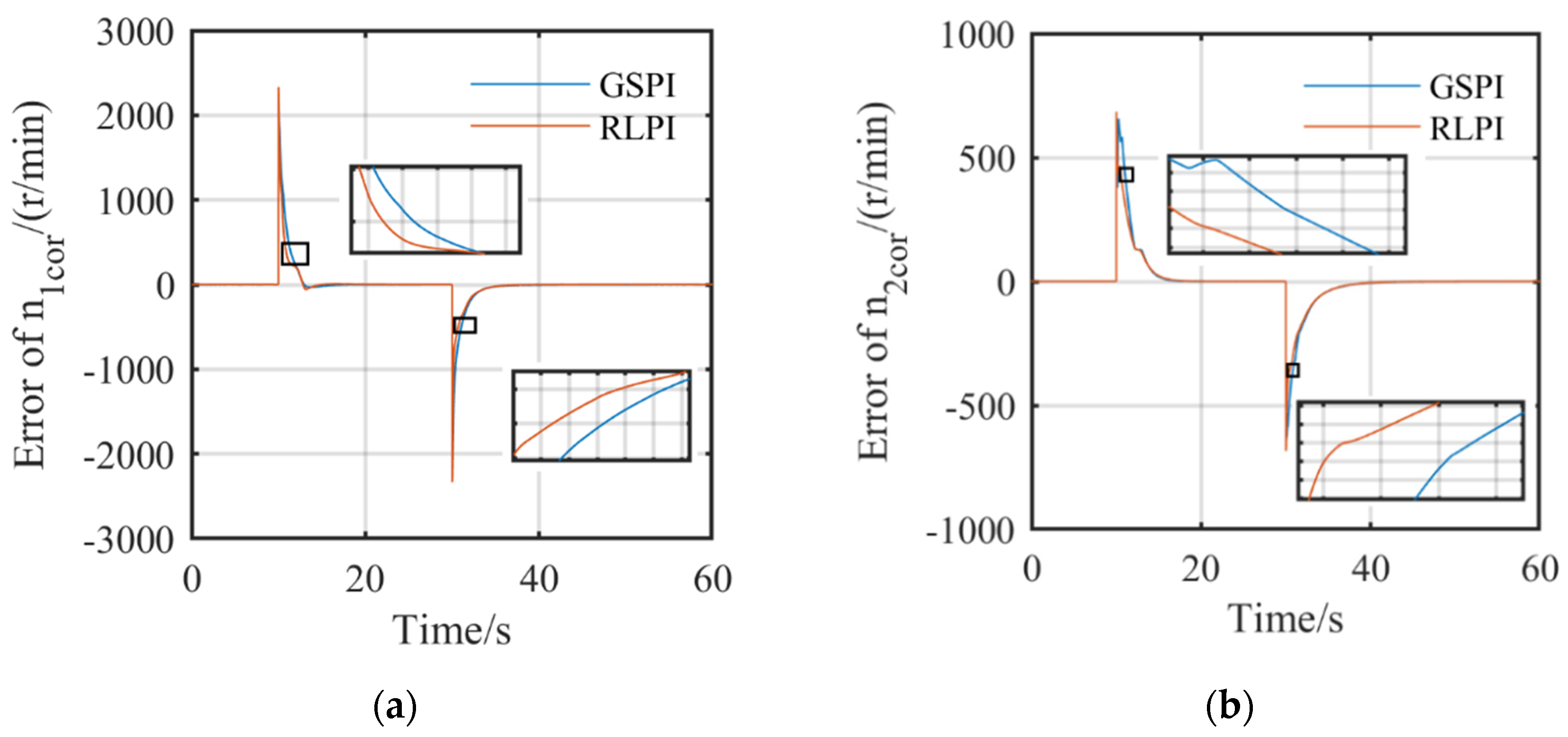
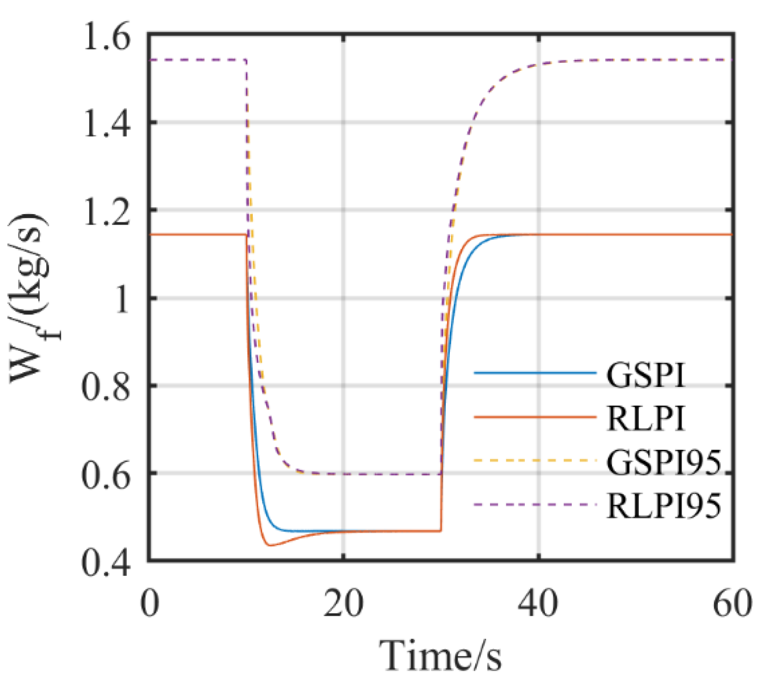
5.3. Simulation Results with Degradation

Degradation occurs inevitably with the life cycle of the turbofan engine, meaning the system cannot work as effectively as before. Traditionally, more fuel will be consumed to obtain the desired performance.
In this section, the degradation is simulated by reducing the compressor efficiency by 5%. Simulation results are shown in Figure 9, Figure 10 and Figure 11 and Table 3. It can be concluded that the transient performance of the system decreases when the efficiency of the compressor decreases for both deceleration and acceleration processes compared with ideal conditions. It is shown in Figure 10 that the maximum difference in n1cor is about 300 r/min and the maximum difference in n2cor is about 100 r/min. The n1cor change with GSPI is smaller than that with RLPI, and the n2or change with RLPI is smaller than that with GSPI. Moreover, it is shown in Figure 9 that the response of the corrected rotor speed is smoother with RLPI, due to the nonlinearity of RLPI. The transient process with RLPI also has faster transient response and smaller transient error.
Cumulative error is used as a criterion of servo tracking, which represents the performance of transient control. The result is shown in Figure 12, where cumulative error (CE) is defined as follows:
C E = ( n n c m d ) / n
where ncmd is the command. The results show that the cumulative error of both GSPI and RLPI increases, but the cumulative error of RLPI is much better. For n1cor, the performance of the turbofan controlled with the RLPI controller after degradation is almost equal to the performance of the turbofan controlled with the GSPI controller before degradation.
The results in Figure 13 show that when the components’ efficiency decreases, more fuel is needed to keep the engine working at the desired speed. It is also illustrated in Figure 13 that the system with RLPI reduces fuel flow faster during deceleration, and adds fuel faster during acceleration. This explains the results, where RLPI tracked the command better in all conditions. It should also be noted that the surge margin (SM) [26] reduces from 17.17 to 12.19 when the degradation takes place.
The comparison of settling time under different conditions is shown in Figure 14, where the solid lines represent the performance with GSPI and the dotted lines represent the performance with RLPI. In the case of settling time, the RLPI has similar performance to GSPI. However, as noted above, the GSPI has better ability in terms of command tracking.

6. Conclusions

This paper presents a method of designing a reinforcement learning controller for turbofan engines. A nonlinear model of the engine was developed as the environment for the reinforcement training process. A DDPG algorithm with actor–critic architecture and a traditional control structure—which was PI in this paper—is presented. The performance of the designed RLPI controller was verified under the chosen conditions and compared with GSPI controllers. The simulation results show that the closed-loop system with the RLPI controller has the desired performance in the transient process. Additionally, the RLPI controller’s ability to deal with large uncertainties and degradation is proven by comparing the simulation results of actuators’ uncertainties, and by compressor efficiency decreasing with the ideal condition.
Studies that should be carried out in the future are as follows: Firstly, the fuel flow and nozzle area need to be trained together in order to achieve better performance, but the training process will be harder to converge. Secondly, different working conditions in the flight envelope should be considered with all-round simulation. Thirdly, control structures other than PI should also be validated in the future. Finally, it is expected that experiments could be carried out with real engines in the future.

Author Contributions

Conceptualization, K.M. and X.W.; methodology, K.M. and X.W.; software, K.M., M.Z. and S.Y.; validation, K.M., M.Z., S.Y. and Z.J.; writing—original draft preparation, K.M.; writing—review and editing, K.M., M.Z. and X.P.; visualization, K.M.; supervision, M.Z.; project administration, X.W. All authors have read and agreed to the published version of the manuscript.

Funding

This research was funded by AECC Sichuan Gas Turbine Establishment Stable Support Project, grant number GJCZ-0011-19, and by the National Science and Technology Major Project, grant number 2017-V-0015-0067.

Institutional Review Board Statement

Not applicable.

Informed Consent Statement

Not applicable.

Data Availability Statement

Not applicable.

Conflicts of Interest

The authors declare no conflict of interest.

References

  1. Zhu, M.; Wang, X.; Dan, Z.; Zhang, S.; Pei, X. Two freedom linear parameter varying μ synthesis control for flight environment testbed. Chin. J. Aeronaut. 2019, 32, 1204–1214. [Google Scholar] [CrossRef]
  2. Zhu, M.; Wang, X.; Miao, K.; Pei, X.; Liu, J. Two Degree-of-freedom μ Synthesis Control for Turbofan Engine with Slow Actuator Dynamics and Uncertainties. J. Phys. Conf. Ser. 2021, 1828, 012144. [Google Scholar] [CrossRef]
  3. Gu, N.N.; Wang, X.; Lin, F.Q. Design of Disturbance Extended State Observer (D-ESO)-Based Constrained Full-State Model Predictive Controller for the Integrated Turbo-Shaft Engine/Rotor System. Energies 2019, 12, 4496. [Google Scholar] [CrossRef] [Green Version]
  4. Dan, Z.H.; Zhang, S.; Bai, K.Q.; Qian, Q.M.; Pei, X.T.; Wang, X. Air Intake Environment Simulation of Altitude Test Facility Control Based on Extended State Observer. J. Propuls. Technol. 2020; in press. [Google Scholar]
  5. Zhu, M.; Wang, X.; Pei, X.; Zhang, S.; Liu, J. Modified robust optimal adaptive control for flight environment simulation system with heat transfer uncertainty. Chin. J. Aeronaut. 2021, 34, 420. [Google Scholar] [CrossRef]
  6. Miao, K.Q.; Wang, X.; Zhu, M.Y. Full Flight Envelope Transient Main Control Loop Design Based on LMI Optimization. In Proceedings of the ASME Turbo Expo 2020, Virtual Online, 21–25 September 2020. [Google Scholar]
  7. Gu, B.B. Robust Fuzzy Control for Aeroengines; Nanjing University of Aeronautics and Astronautics: Nanjing, China, 2018. [Google Scholar]
  8. Amgad, M.; Shakirah, M.T.; Suliman, M.F.; Hitham, A. Deep-Learning Based Prognosis Approach for Remaining Useful Life Prediction of Turbofan Engine. Symmetry 2021, 13, 1861. [Google Scholar] [CrossRef]
  9. Zhang, X.H.; Liu, J.X.; Li, M.; Gen, J.; Song, Z.P. Fusion Control of Two Kinds of Control Schedules in Aeroengine Acceleration Process. J. Propuls. Technol. 2021; in press. [Google Scholar]
  10. Yin, X.; Shi, G.; Peng, S.; Zhang, Y.; Zhang, B.; Su, W. Health State Prediction of Aero-Engine Gas Path System Considering Multiple Working Conditions Based on Time Domain Analysis and Belief Rule Base. Symmetry 2022, 14, 26. [Google Scholar] [CrossRef]
  11. Frank, L.L.; Draguna, V.; Kyriakos, G.V. Reinforcement learning and feedback control. IEEE Control Syst. Mag. 2012, 32, 76–105. [Google Scholar]
  12. Sutton, R.S.; Barto, A.G. Reinforcement Learning: An Introduction; MIT Press: Cambridge, MA, USA, 1998. [Google Scholar]
  13. Lillicrap, T.P.; Hunt, J.J.; Pritzel, A.; Heess, N.; Erez, T.; Tassa, Y.; Silver, D.; Wierstra, D. Continuous control with deep reinforcement learning. arXiv 2016, arXiv:1509.02971. [Google Scholar]
  14. Richard, S.S.; David, M.; Satinder, S.; Yishay, M. Policy Gradient Methods for Reinforcement Learning with Function Approximation. Adv. Neural Inf. Process. Syst. 2000, 12, 1057–1063. [Google Scholar]
  15. Silver, D.; Lever, G.; Heess, N.; Degris, T.; Wierstra, D.; Riedmiller, M. Deterministic Policy Gradient Algorithms. In Proceedings of the International Conference on Machine Learning, Bejing, China, 22–24 June 2014; pp. 387–395. [Google Scholar]
  16. Giulia, C.; Shreyansh, D.; Roverto, C. Learning Transferable Policies for Autonomous Planetary Landing via Deep Reinforcement Learning. In Proceedings of the ASCEND, Las Vegas, NV, USA, 15–17 November 2021. [Google Scholar]
  17. Sun, D.; Gao, D.; Zheng, J.H.; Han, P. Reinforcement learning with demonstrations for UAV control. J. Beijing Univ. Aeronaut. Astronaut. 2021; in press. [Google Scholar]
  18. Kirk, H.; Steve, U. On Deep Reinforcement Learning for Spacecraft Guidance. In Proceedings of the AIAA SciTech Forum, Orlando, FL, USA, 6–10 January 2020. [Google Scholar]
  19. Hiroshi, K.; Seiji, T.; Eiji, S. Feedback Control of Karman Vortex Shedding from a Cylinder using Deep Reinforcement Learning. In Proceedings of the AIAA AVIATION Forum, Atlanta, GA, USA, 25–29 June 2018. [Google Scholar]
  20. Hu, X. Design of Intelligent Controller for Variable Cycle Engine; Dalian University of Technology: Dalian, China, 2020. [Google Scholar]
  21. Li, Y.; Nie, L.C.; Mu, C.H.; Song, Z.P. Online Intelligent Optimization Algorithm for Adaptive Cycle Engine Performance. J. Propuls. Technol. 2021, 42, 1716–1724. [Google Scholar]
  22. Wang, F. Research on Prediction of Civil Aero-Engine Gas Path Health State And Modeling Method of Spare Engine Allocation; Harbin Institute of Technology: Harbin, China, 2020. [Google Scholar]
  23. Li, Z. Research on Life-Cycle Maintenance Strategy Optimization of Civil Aeroengine Fleet; Harbin Institute of Technology: Harbin, China, 2019. [Google Scholar]
  24. Richter, H. Advanced Control of Turbofan Engines; National Defense Industry Press: Beijing, China, 2013; p. 16. [Google Scholar]
  25. Miao, K.Q.; Wang, X.; Zhu, M.Y. Dynamic Main Close-loop Control Optimal Design Based on LMI Method. J. Beijing Univ. Aeronaut. Astronaut. 2021; in press. [Google Scholar]
  26. Zeyan, P.; Gang, L.; Xingmin, G.; Yong, H. Principle of Aviation Gas Turbine; National Defense Industry Press: Beijing, China, 2008; p. 111. [Google Scholar]
Figure 1. The structure of reinforcement learning.
Symmetry 14 00684 g001
Figure 2. The training process with DDPG.
Symmetry 14 00684 g002
Figure 3. Actor–critic reinforcement learning framework.
Symmetry 14 00684 g003
Figure 4. Relationships of the neural networks in the actor–critic framework.
Symmetry 14 00684 g004
Figure 5. Framework of a traditional feedback control system and a feedback control system based on reinforcement learning.
Symmetry 14 00684 g005
Figure 6. Improved framework of a feedback control system based on reinforcement learning with a DDPG algorithm.
Symmetry 14 00684 g006
Figure 7. Nozzle area command.
Symmetry 14 00684 g007
Figure 8. Response of corrected rotor speed with RLPI controllers with different time constants: (a) Comparison of n1cor response. (b) Comparison of n2cor response.
Symmetry 14 00684 g008
Figure 9. Response of corrected rotor speed with GSPI and RLPI controllers before and after degradation: (a) Comparison of n1cor response. (b) Comparison of n2cor response.
Symmetry 14 00684 g009
Figure 10. Difference in corrected rotor speed control performance with GSPI and RLPI controllers before and after degradation: (a) Difference in n1cor control performance before and after degradation. (b) Difference in n2cor control performance before and after degradation.
Symmetry 14 00684 g010
Figure 11. Corrected rotor speed error with GSPI and RLPI controllers when degradation takes place: (a) Comparison of n1cor response error. (b) Comparison of n2cor response error.
Symmetry 14 00684 g011
Figure 12. Cumulative error in the transient process under different conditions.
Symmetry 14 00684 g012
Figure 13. Comparison of Wf with the GSPI and RLPI controllers under different conditions.
Symmetry 14 00684 g013
Figure 14. Comparison of settling time under different conditions.
Symmetry 14 00684 g014
Table 1. Training options.
FunctionDescriptionValue
Critic Representation OptionsLearn Rate0.001
Gradient Threshold1
Actor Representation OptionLearn Rate0.0001
Gradient Threshold1
DDPG Agent OptionsSample time0.01
Target Smooth Factor0.003
Discount Factor1
Mini-Batch Size64
Experience Buffer Length1,000,000
Noise Options Variance0.3
Noise Options’ Variance Decay Rate0.00001
Training OptionsSample time0.01
Maximum Episodes20,000
Maximum Steps per Episode1000
Score-Averaging Window Length2
Stop Training Value996
Table 2. Performance of the system with an RLPI controller in different conditions.
τaSpeedTs/sσ%State
0.1n1cor1.430Acceleration
2.231.50Deceleration
n2cor3.840Acceleration
3.330Deceleration
0.2n1cor1.180Acceleration
2.902.23Deceleration
n2cor3.710Acceleration
3.150Deceleration
Table 3. Performance of the systems with GSPI and RLPI controllers when degradation takes place.
ControllerSpeedTs/sσ%State
GSPIn1cor2.670Acceleration
3.780.39Deceleration
n2cor5.310Acceleration
3.170Deceleration
RLPIn1cor2.530Acceleration
4.400.75Deceleration
n2cor5.270Acceleration
4.500Deceleration
Publisher’s Note: MDPI stays neutral with regard to jurisdictional claims in published maps and institutional affiliations.

