Article

A Stochastic Discrete Empirical Interpolation Approach for Parameterized Systems

1
School of Information Science and Technology, ShanghaiTech University, Shanghai 201210, China
2
College of Natural Resources and Environment, Northwest A&F University, Xianyang 712100, China
*
Author to whom correspondence should be addressed.
Symmetry 2022, 14(3), 556; https://doi.org/10.3390/sym14030556
Submission received: 15 February 2022 / Revised: 4 March 2022 / Accepted: 5 March 2022 / Published: 10 March 2022
(This article belongs to the Special Issue Symmetry in Functional Equations and Analytic Inequalities III)

Abstract

:
As efficient separation of variables plays a central role in model reduction for nonlinear and nonaffine parameterized systems, we propose a stochastic discrete empirical interpolation method (SDEIM) for this purpose. In our SDEIM, candidate basis functions are generated through a random sampling procedure, and the dimension of the approximation space is systematically determined by a probability threshold. This random sampling procedure avoids large candidate sample sets for high-dimensional parameters, and the probability based stopping criterion can efficiently control the dimension of the approximation space. Numerical experiments are conducted to demonstrate the computational efficiency of SDEIM, which include separation of variables for general nonlinear functions, e.g., exponential functions of the Karhu nen–Loève (KL) expansion, and constructing reduced order models for FitzHugh–Nagumo equations, where symmetry among limit cycles is well captured by SDEIM.

1. Introduction

When conducting model reduction for nonlinear and nonaffine parameterized systems [1], separation of variables is an important step. During the last few decades, many strategies have been developed to achieve this goal, e.g., empirical interpolation methods (EIM) [2,3,4,5], discrete empirical interpolation methods (DEIM) [6,7], and variable-separation (VS) methods [8]. To result in an accurate linear representation, these methods typically need a fine reduced basis approximation space. To construct the corresponding basis functions, repeated evaluations of expensive parameterized systems are required. The accuracy of the EIM/DEIM approximations depends on candidate parameter samples. Properly choosing the samples is crucial and is especially challenging when the parameter space is high dimensional.
For reduced basis approximations [9,10,11,12,13,14], the work in [15] shows that candidate sample sets for reduced bases can be chosen as a random set of a specified order and the resulting approximation satisfies given accuracies with a probability threshold. Rather than reduced basis approximations, we in this paper focus on separation of variables for nonlinear and nonaffine systems, and propose a stochastic discrete empirical interpolation method (SDEIM). In our SDEIM, the interpolation is processed through two steps: the first is to randomly select sample points to construct an approximation space for empirical interpolation, and the second is to evaluate if the approximation accuracy meets the probability threshold on additional samples. These two steps are repeated until the approximation space satisfies the given accuracy and probability requirements. The probability correctness of the approximation space is reassessed by SDEIM each time the approximation space is updated. We note that SDEIM does not loop over a fine candidate sample set, which significantly reduces the computational cost for empirical interpolation for high-dimensional systems. To demonstrate the efficiency of SDEIM, we utilize it to approximate test functions including the exponential functions of the Karhu nen–Loève (KL) expansion, which is widely used to parameterize random fields. Finally, we use SDEIM to solve ordinary differential equations (ODEs) arising from the FitzHugh–Nagumo (F–N) system [6,16], and all these results show that SDEIM is efficient. It is worth noting that many natural phenomena can have symmetric properties, and symmetry of limit cycles of the F-N system is well captured by SDEIM.
An outline of the paper is as follows. We first present our problem setting, and then review the fine collateral reduced-basis approximation space and EIM in Section 2. After a short introduction of the discrete form, we present SDEIM and analyze its performance in Section 3. Numerical results are discussed in Section 4. Finally, we conclude the paper in Section 5.

2. Problem Formulation

Nonlinear terms and functions in complex systems cause significant difficulties for efficient model reduction, and separation of variables is typically required. In this section, we refer to nonlinear functions under consideration as the target functions. Let Ω R d (for d = 1 , 2 or 3) be a bounded, connected physical domain and Γ be a high dimensional parameter space. The target function with a general form is written as
ξ f ( x , ξ ) , x Ω , ξ Γ .
The target function f ( x , ξ ) is assumed to be nonlinear. In the following, we review EIM [2], which is to approximate f ( x , ξ ) with a separate representation for x and ξ .

2.1. The Linear Approximation Space

Before introducing EIM, we first introduce its fine collateral reduced-basis approximation space following [2,6,17,18]. Without loss of generality, we assume that the target function f ( x , ξ ) is uniquely defined in some Hilbert space H for every ξ Γ . An inner product and a L 2 norm of H are denoted as < f , g > : = Ω f ( x , ξ ) g ( x , ξ ) d x and · : = < · , · > . We define the target manifold M as
M : = f ( x , ξ ) | ξ Γ .
when the target manifold M has a low dimension, a low dimensional linear space can approximate it well. The infimum of the supremum distance between the n-dimensional linear approximation space and the target manifold M is called the Kolmogorov n-width [3,19], which is defined as
κ n = κ n ( M ) : = inf dim ( V ) = n sup ξ Γ f ( x , ξ ) P V f ( x , ξ ) .
Here, P V denotes the orthogonal projection onto V , where V is an arbitrary linear space, i.e.,
< P V f ( x , ξ ) , f ( x , ξ ) P V f ( x , ξ ) > = 0 .
Moreover, from (2) we can get the property
P V f ( x , ξ ) 2 = < P V f ( x , ξ ) , P V f ( x , ξ ) > = f ( x , ξ ) , f ( x , ξ ) f ( x , ξ ) P V f ( x , ξ ) , f ( x , ξ ) P V f ( x , ξ ) = f ( x , ξ ) 2 f ( x , ξ ) P V f ( x , ξ ) 2 f ( x , ξ ) 2 .
Since the orthogonal projection is linear, (3) means that the error is reduced after the orthogonal projection. However, the space satisfying (1) is nontrivial to reach. The work in [20] has proposed a specific greedy procedure for constructing this n dimensional linear approximation space which optimizes
κ ˜ n : = inf dim ( V ) = n sup ξ Γ train f ( x , ξ ) P V f ( x , ξ )
instead of κ n in a sufficiently fine candidate sample set Γ train Γ . Since the candidate set Γ train contains a finite number of samples, optimizing κ ˜ n is equivalent to search ξ ( k ) such that
ξ ( k ) = argmax ξ Γ train f ( x , ξ ) P V f ( x , ξ ) .
Then, we update the linear approximation space V for this target function f x , ξ ( k ) . A greedy procedure which constructs a linear approximation space V satisfying κ ˜ n t o l 3 , where t o l is a given tolerance, can be stated as follows. First this procedure initializes the linear approximation space V 0 : = span { 0 } . Then, it selects a new parameter value by
ξ ( k + 1 ) : = argmax ξ Γ train f ( x , ξ ) P V k f ( x , ξ ) .
If the error
η ˜ ξ ( k + 1 ) = f x , ξ ( k + 1 ) P V k f x , ξ ( k + 1 )
is greater than t o l 3 , we update the linear approximation space V k + 1 = span V k f x , ξ ( k + 1 ) . At the end of this procedure, the linear approximation space V is set to V = V n and V satisfies η ˜ ( ξ ) t o l 3 for all ξ Γ train . Moreover, that the candidate sample set Γ train is sufficiently fine means that the discrete target manifold
M ˜ = f ( x , ξ ) | ξ Γ train
is a t o l 3 -approximation net for target manifold M , i.e.,
d ( M , M ˜ ) : = sup ξ Γ inf ξ ˜ Γ train f ( x , ξ ) f ( x , ξ ˜ ) t o l 3 .
Then for any ξ Γ , (3) and (5) give
f ( x , ξ ) P V f ( x , ξ ) inf ξ ˜ Γ train ( f ( x , ξ ) f ( x , ξ ˜ ) + f ( x , ξ ˜ ) P V f ( x , ξ ˜ ) + P V f ( x , ξ ˜ ) P V f ( x , ξ ) ) 2 inf ξ ˜ Γ train f ( x , ξ ) f ( x , ξ ˜ ) + t o l 3 2 t o l 3 + t o l 3 = t o l .
The inequality (6) means that the standard greedy procedure with a fine candidate sample set Γ train can generate a linear approximation space which approximates the target manifold M with any tolerance t o l .

2.2. Empirical Interpolation Method (EIM)

Section 2.1 explains that, when the candidate sample set Γ train is fine enough, the greedy procedure can produce a linear approximation space V which is a t o l -approximation space for the original target manifold M , i.e.,
sup f ( x , ξ ) M f ( x , ξ ) P V f ( x , ξ ) t o l .
For this linear approximation space V , if we denote a set of orthonormal basis functions of V as ϕ 1 ( x ) , , ϕ n ( x ) , the orthogonal projection P V can be expressed as
P V f ( x , ξ ) = i = 1 n β i ( ξ ) ϕ i ( x ) .
Here, β i ( ξ ) R , i = 1 , , n , are the coefficients corresponding to the basis function ϕ i ( x ) . Since the basis functions ϕ i ( x ) , i = 1 , , n are orthonormal, the coefficient β i can be calculated by
β i ( ξ ) = < f ( x , ξ ) , ϕ i ( x ) > = Ω f ( x , ξ ) ϕ i ( x ) d x , i , 1 i n .
However, in order to get the coefficient β i ( ξ ) in (9), we need to evaluate an integration with target function f ( x , ξ ) , which is inconvenient.
The interpolation method [2,18,21] is widely used in function approximation. It approximates the target function f ( x , ξ ) by restricting the values of this function on n interpolation points x ( 1 ) , , x ( n ) Ω . If we denote the approximation function as I Ω f ( x , ξ ) f ( x , ξ ) , the restrictions are
I Ω f x ( i ) , ξ = f x ( i ) , ξ , ξ Γ , i , 1 i n .
In addition, if we approximate the target function f ( x , ξ ) using interpolation methods in a linear approximation space V , and denote it as I V f ( x , ξ ) , then (8) and (10) can be written as
I V f x ( i ) , ξ = i = 1 n β i ( ξ ) ϕ i x ( i ) = f x ( i ) , ξ , ξ Γ , i , 1 i n .
Here, β i ( ξ ) , i = 1 , , n , are the unknown coefficients. Moreover, we denote the matrix Φ R n × n as
Φ = ϕ 1 x ( 1 ) ϕ n x ( 1 ) ϕ 1 x ( n ) ϕ n x ( n ) .
Then, the coefficient β ̲ ( ξ ) : = β 1 ( ξ ) , , β n ( ξ ) T satisfying (11) is the solution of the linear system
Φ β ̲ ( ξ ) = ϕ 1 x ( 1 ) ϕ n x ( 1 ) ϕ 1 x ( n ) ϕ n x ( n ) β 1 ( ξ ) β n ( ξ ) = i = 1 n β i ( ξ ) ϕ i x ( 1 ) i = 1 n β i ( ξ ) ϕ i x ( n ) = f x ( 1 ) , ξ f x ( n ) , ξ .
Compared with (9), β ̲ which is evaluated by the interpolation method (12) avoids the integration and only needs to know the value of target function f ( x , ξ ) on n interpolation points x ( 1 ) , , x ( n ) . The target function f ( x , ξ ) can then be approximated by
f ( x , ξ ) I V f ( x , ξ ) = i = 1 n β i ( ξ ) ϕ i ( x ) ,
where the coefficients β i ( ξ ) , i = 1 , , n are the solution of (12). Then, (13) naturally satisfies the restriction (11) by the definition of the coefficients β i ( ξ ) , i = 1 , , n .
In EIM [2,3,17,21], systematical approaches to choose suitable interpolation points are given. Here, approximation basis functions and interpolation points are typically obtained alternately by minimizing the error between the target function f ( x , ξ ) and its approximation function I V f ( x , ξ ) , of which the produce can be summarized as follows. First, we initialize V 0 = span 0 , and select a new parameter value as
ξ ( k + 1 ) : = argmax ξ Γ train f ( x , ξ ) I V k f ( x , ξ ) .
For the parameter value ξ ( k + 1 ) , if the error
η ξ ( k + 1 ) = f x , ξ ( k + 1 ) I V k f x , ξ ( k + 1 )
is greater than t o l , the linear approximation space is updated as V k + 1 = span V k f x , ξ ( k + 1 ) . Then, we orthonormalize the target function f x , ξ ( k + 1 ) with the basis functions ϕ 1 ( x ) , , ϕ k ( x ) by Schmidt orthogonalization for numerical stability and denote it as ϕ k + 1 ( x ) , i.e.,
e ( x ) = f x , ξ ( k + 1 ) i = 1 k f x , ξ ( k + 1 ) , ϕ i ( x ) ϕ i ( x ) , ϕ k + 1 ( x ) = e ( x ) e ( x ) ,
where f x , ξ ( k + 1 ) , ϕ i ( x ) , i = 1 , 2 , , k , are the coefficients of the projection of f x , ξ ( k + 1 ) over V k = span ϕ 1 ( x ) , ϕ 2 ( x ) , , ϕ k ( x ) . The next interpolation point is selected by maximizing the absolute value of the error r k ( x ) = ϕ k + 1 ( x ) I V k ϕ k + 1 ( x ) , i.e.,
x ( k + 1 ) = argmax x Ω | r k ( x ) | .
The above procedure is repeated until the error η ( ξ ) t o l (see (14)) for all ξ Γ train , and we denote V = V n for the final step. The relationship between the error f x , ξ I V f x , ξ and f x , ξ P V f x , ξ are discussed in [2] (see [6] for its discrete version).

3. Discrete Empirical Interpolation Method and Its Stochastic Version

We evaluate the values of f x , ξ ( k ) on a discrete physical domain, that is, computing a vector function
ξ f h ( ξ ) ,
where f h ( ξ ) = f x ( 1 ) , ξ , , f x ( N h ) , ξ T with N h components is the discrete version of f x , ξ on N h physical points x ( 1 ) , , x ( N h ) . The number of discrete points N h is usually large to meet certain appropriation accuracy. On the other hand, since the physical domain has been discretized, selecting interpolation points is to find proper indices from 1 , 2 , , N h . If i 1 , , i n denote the indices of the interpolation points and P R N h × n denote the matrix of interpolation points defined as
P = [ e i 1 , , e i n ]
with e i R N h × 1 the i-th canonical unit vector, the values of target function f h ( ξ ) on the interpolation points can be written as P T f h ( ξ ) . As a result, the corresponding interpolation only needs the values of f h ( ξ ) on i 1 , , i n components with n N h .

3.1. Discrete Empirical Interpolation Method (DEIM)

Before presenting our stochastic discrete empirical interpolation method, we here review the original DEIM [6]. In the discrete formulation, a linear approximation space V can be expressed as
V = span f h ξ ( 1 ) , , f h ξ ( n ) ,
which is an approximation of the discrete target manifold
M h = f h ( ξ ) | ξ Γ .
Denoting a set of orthonormal basis functions of this linear approximation space V by q i R N h × 1 , i = 1 , 2 , , n , and denoting the matrix of basis functions by Q = [ q 1 , , q n ] R N h × n , the approximation of the target function f h ( ξ ) corresponding to (8) can be written as
f h ( ξ ) f ^ h : = Q β ̲ ( ξ ) = i = 1 n β i ( ξ ) q i ,
where β ̲ ( ξ ) = ( β 1 , , β n ) T is the coefficient. The restriction of interpolation points corresponding to (13) is
P T f h ( ξ ) = P T Q β ̲ ( ξ ) ,
which gives β ̲ ( ξ ) = P T Q 1 P T f h ( ξ ) . Then, it can naturally derive
f ^ h ( ξ ) = Q β ̲ ( ξ ) = Q P T Q 1 Q ˜ P T f h ( ξ ) β ̲ ˜ ( ξ ) .
By the way β ̲ is obtained, the values of the approximation function f ^ h ( ξ ) are equal to the target function f h ( ξ ) on the components i 1 , , i n for any ξ Γ , i.e., P T f ^ h ( ξ ) = P T f h ( ξ ) . Moreover, the calculation of the new matrix of basis functions Q ˜ = Q P T Q 1 R N h × n is required once only. For a new realization ξ , DEIM only computes the values of the target function f h ( ξ ) on the components i 1 , , i n as the new coefficient β ̲ ˜ ( ξ ) = P T f h ( ξ ) R n × 1 .
The procedure of DEIM to construct a linear approximation space and select interpolation points can be stated as follows. For a fine candidate sample set Γ train , it first chooses
ξ ( 1 ) = argmax ξ Γ train f h ( ξ ) 2 ,
where · 2 is the vector L 2 norm for a discrete function. Then, we orthonormalize f h ξ ( 1 ) as q 1 and denote Q 1 = [ q 1 ] with
q 1 : = f h ξ ( 1 ) f h ξ ( 1 ) 2 .
The index of the first interpolation point i 1 is initialized as
i 1 = argmax i = 1 , , N h | e i T q 1 | ,
and we let P 1 = [ e i 1 ] . For the ( k + 1 ) -th basis function and interpolation point, a parameter value ξ ( k + 1 ) is chosen from the candidate sample set Γ train by finding the maximum error between the target function f h ( ξ ) and its approximation f ^ h ( ξ ) in the linear approximation space V k = span { q 1 , , q k } , i.e.,
ξ ( k + 1 ) = argmax ξ Γ train f h ( ξ ) f ^ h ( ξ ) 2 .
If the error η ξ ( k + 1 ) = f h ξ ( k + 1 ) f ^ h ξ ( k + 1 ) 2 is greater than a given tolerance t o l , we orthonormalize f h ξ ( k + 1 ) with q 1 , , q k by Schmidt orthogonalization and denote it as q k + 1 , that is,
e ( k + 1 ) : = f h ξ ( k + 1 ) Q k Q k T f h ξ ( k + 1 ) , q ( k + 1 ) : = e ( k + 1 ) e ( k + 1 ) 2 .
Then, the matrix of basis functions is updated as Q k + 1 = [ Q k , q k + 1 ] . The residual of interpolation projecting q k + 1 to the linear approximation space V k can be written as
r k : = q k + 1 q ^ k + 1 = q k + 1 Q k P k T Q k 1 P k T q k + 1 .
An index of ( k + 1 ) -th interpolation point i k + 1 is selected by finding the maximum component of residual r k , i.e.,
i k + 1 = argmax i = 1 , , N h | e i T r k | ,
and we update P k + 1 = [ P k , e i k + 1 ] . Finally, we denote V = V n , Q = Q n and P = P n . This linear approximation space V then satisfies
sup ξ Γ train f h ( ξ ) f ^ h ( ξ ) 2 t o l .
The whole procedure is stated in Algorithm 1, where η means the error in (14) or its discrete form (17).
Algorithm 1 Discrete empirical interpolation method (DEIM) [6]
Input: A candidate sample set Γ train and a target function f h ( ξ ) .
1: Initialize ξ ( 1 ) = argmax ξ Γ train f h ( ξ ) 2 and orthonormalize f h ξ ( 1 ) as q 1 = f h ξ ( 1 ) / f h ξ ( 1 ) 2 .
2: Initialize i 1 = argmax i = 1 , , N h | e i T q 1 | .
3: Initialize Q = [ q 1 ] and P = [ e i 1 ] .
4: while sup ξ Γ train η ( ξ ) = f h ( ξ ) f ^ h ( ξ ) 2 > t o l do
5:   Compute the error η ξ ( i ) for ξ ( i ) Γ train , i = 1 , 2 , , | Γ train | .
6:   Let ξ ( k + 1 ) = argmax ξ Γ train η ξ .
7:   Compute q k + 1 through orthonormalizing f h ξ ( k + 1 ) with q 1 , , q k by (18).
8:   Solve the equation P T q k + 1 = P T Q β ̲ for β ̲ .
9:   Compute the residual r k = q k + 1 q ^ k + 1 = q k + 1 Q β ̲ .
10:    Select the interpolation index i k + 1 as i k + 1 = argmax i = 1 , , N h | e i T r k | .
11:    Update Q = [ Q , q k + 1 ] and P = [ P , e i k + 1 ] .
12: end while
Output: The matrix of basis functions Q and the matrix of interpolation points P .

3.2. Stochastic Discrete Empirical Interpolation Method (SDEIM)

For standard EIM (or DEIM), to satisfy the t o l -approximation (see (7)), the candidate sample set Γ train typically needs to be fine enough (i.e., the condition (5) holds). However, if the size of Γ train is large, it can be expensive to construct the DEIM approximation (15). In this section, we propose a stochastic discrete empirical interpolation method (SDEIM). In SDEIM, we accept the approximation with probability instead of giving a threshold with certainty, and we then avoid fine candidate sample sets. We note that a weight EIM strategy is developed in [4], while the purpose of our work is to give a stochastic criterion for updating training sets.
Our problem formulation is still to approximate the target manifold M h with a linear approximation space V , such that it satisfies
η ( ξ ) = f h ( ξ ) I V f h ( ξ ) 2 t o l .
However, assuming that a probability measure P exists in the parameter space Γ , we herein do not ensure η ( ξ ) t o l for all ξ Γ , but concern about the failure probability
p : = P ξ Γ | η ( ξ ) > t o l ,
which measures the size of the parameter set where the approximation is not accurate enough. While the probability p can hardly be exactly evaluated, we evaluate its empirical probability among N samples
p ¯ : = 1 N i = 1 N I η ξ ( i ) t o l ,
where I ( x ) is the indicator function defined as
I ( x ) = 1 , if x > 0 , 0 , if x 0 .
The probability (22) is to calculate the average number of occurrences of η ( ξ ) > t o l on N samples. By the law of large numbers [22], the empirical probability p ¯ converges to the probability p with probability one as N goes to infinite, i.e.,
P lim N 1 N i = 1 N I η ξ ( i ) t o l = p = 1 .
Since the implicit constant p reflects the probability that ξ does not satisfy the tolerance t o l , we hope that p is small enough. On the other hand, p can not be evaluated explicitly, and the empirical probability p ¯ is an approximation of p. In SDEIM, therefore, p ¯ is set to be small enough. For convenience, we take p ¯ = 0 in the verifying stage and use the sample size N to control the accuracy of p ¯ to approximate p.
The procedure of SDEIM has two steps: constructing a linear approximation space V , and verifying whether the empirical probability p ¯ = 0 for this linear approximation space V in N consecutive samples. Our SDEIM algorithm can be described as follows. First, a sample ξ ( 1 ) Γ is randomly selected, and the target function f h ξ ( 1 ) is normalized as q 1 . The linear approximation space is initialized as V 1 = span { q 1 } and the matrix of basis function is denoted as Q 1 = [ q 1 ] . The index of the first interpolation point i 1 is initialized in the same way as (16) and the matrix of interpolation point is denoted as P 1 = [ e i 1 ] . Then, the empirical probability p ¯ is verified for this linear approximation space V 1 . We sample N consecutive samples. If one of these N samples makes η ( ξ ) > t o l , we orthonormalize q k + 1 for this sample ξ , find the index of the ( k + 1 ) -th interpolation point i k + 1 as DEIM in (19) and (20) and update P k + 1 = [ P k , e i k + 1 ] . The linear approximation space is updated as V k + 1 = span V k q k + 1 and the matrix of the basis function is updated as Q k + 1 = [ Q k , q k + 1 ] . Then, the empirical probability p ¯ is verified again for this linear approximation space V k + 1 . The above steps are repeated alternately until there is a linear approximation space V n such that η ( ξ ( i ) ) t o l for N consecutive samples. Finally, a linear approximation space V = V n is obtained, such that the empirical probability p ¯ = 0 for N consecutive samples. Details of SDEIM are stated as Algorithm 2.
Algorithm 2 Stochastic discrete empirical interpolation method (SDEIM)
Input: A constant number N and a target function f h ( ξ ) .
1: Sample ξ randomly.
2: Evaluate the target function f h ( ξ ) and initialize q 1 = f h ( ξ ) / f h ( ξ ) 2 .
3: Initialize i 1 = argmax i = 1 , , N h | e i T q 1 | .
4: Initialize Q = [ q 1 ] and P = [ e i 1 ] .
5: Initialize the counting index j = 0 .
6: while j N (if j > N , it means that p ¯ = 0 in verifying stage) do
7:  Sample ξ Γ randomly.
8:  if error η ( ξ ) = f h ( ξ ) f ^ h ( ξ ) 2 > t o l then
9:      Set counting index j = 0 .
10:    Compute q k + 1 through orthonormalizing f h ( ξ ) with the q 1 , , q k by (18).
11:    Solve P T q k + 1 = P T Q β ̲ for β ̲ .
12:    Compute the residual r k = q k + 1 q ^ k + 1 = q k + 1 Q β ̲ .
13:    Select the interpolation index i k + 1 as i k + 1 = argmax i = 1 , , N h | e i T r k | .
14:    Update Q = [ Q , q k + 1 ] and P = [ P , e i k + 1 ] .
15:  else
16:    Update j = j + 1 .
17:  end if
18: end while
Output: The matrix of basis functions Q and the matrix of interpolation points P .

3.3. Performance and Complexity of SDEIM

In SDEIM, we ensure that the empirical probability p ¯ = 0 for N consecutive samples in the verifying stage, i.e., the number of ξ such that η ( ξ ) > t o l is zero in these N consecutive samples. The probability p is adjusted through the samples size N, which affects the accuracy of p ¯ for approximating p. For any tolerance t o l and sample size N, there is always a linear approximation space V such that η ( ξ ) = f h ( ξ ) I V f h ( ξ ) 2 t o l for N consecutive samples—in the worst case, when the dimension of the linear approximation space dim ( V ) = N h , this linear approximation space V obviously satisfies the condition.
Although the probability value p cannot be evaluated explicitly, the empirical probability p ¯ approximates the probability p with probability one as N goes to infinite. Hence, for a given threshold ε and a confidence ( 1 δ ) , we can consider this question, whether there is
P | p p ¯ | < ε 1 δ .
By the law of large numbers, the answer is always correct for a suitable N. Before describing the relationship between N and the probability p, the threshold ε and the confidence level ( 1 δ ) , we first introduce the Hoeffding’s inequality as Lemma 1.
Lemma 1
(Hoeffding’s inequality [23]). Let random variables X 1 , X 2 , , X N be independent and identically distributed with values in the interval [ 0 , 1 ] and expectation E X , then for any ε > 0
P E X 1 N i = 1 N X i ε 2 exp 2 N ε 2 , P E X 1 N i = 1 N X i ε exp 2 N ε 2 .
The Hoeffding’s inequality characters the relationship between the arithmetic mean 1 N i = 1 N X i and its expectation E X for bounded random variables. In SDEIM, when a linear approximation space V is given, the error η ( ξ ) can only be greater than tolerance t o l or not greater than t o l for any realization ξ . Hence, the indicator I η ( ξ ) t o l is a random variable taking value of zero or one with expectation E I η ( ξ ) t o l = p . Note that we set the empirical probability p ¯ = 0 in the verifying stage. Then, the problem (23) can be answered with Theorem 1.
Theorem 1.
For any significant level δ ( 0 < δ < 1 ) and threshold ε, the linear approximation space V is produced by SDEIM with sample size N. Then, if N 1 2 ε 2 ln 1 δ , we have
P ( p < ε ) 1 δ .
Proof. 
By Lemma 1 and p ¯ = 0 in SDEIM, we have
P ( p < ε ) = 1 P ( p ε ) = 1 P ( p p ¯ ε ) 1 exp ( 2 N ε 2 ) 1 exp ( 2 ε 2 1 2 ε 2 ln 1 δ ) = 1 δ .
Moreover, the relationship between probability p and the sample size N, the threshold ε , the confidence ( 1 δ ) , can be explicitly described as Theorem 2.
Theorem 2.
For any significance level δ ( 0 < δ < 1 ), the linear approximation space V is produced by SDEIM with sample size N. There is at least confidence ( 1 δ ) satisfying
0 < p < 1 2 N ln 1 δ .
It means that, if the error estimator in SDEIM is set to η ( ξ ) = f h ( ξ ) I V f h ( ξ ) 2 , with confidence ( 1 δ ) , we have
P f h ( ξ ) I V f h ( ξ ) 2 > t o l < 1 2 N ln 1 δ
and
P f h ( ξ ) I V f h ( ξ ) 2 t o l 1 1 2 N ln 1 δ .
Proof. 
Without loss of generality, we set
δ = exp ( 2 N ε 2 )
for suitable ε, that is
ε = 1 2 N ln 1 δ .
By Lemma 1 and p ¯ = 0 in SDEIM, we have
P p 1 2 N ln 1 δ exp ( 2 N ε 2 ) = δ .
That is
p < 1 2 N ln 1 δ
with confidence ( 1 δ ) . In addition, when the error estimator is set to η ( ξ ) = f h ( ξ ) I V f h ( ξ ) 2 , since the definition of p in (21) is
p = P ξ Γ | η ( ξ ) > t o l ,
(24) and (25) can be derived directly. □
Theorem 2 ensures that the linear approximation space V given by the SDEIM algorithm (Agorithm 2), can approximate the target function f h ( ξ ) with the tolerance t o l and the probability threshold ε . Actually, in Algorithm 2, we reset the counting index each time η ( ξ ) > t o l occurs, which means that there are more than N samples such that η ( ξ ) < t o l . Hence, 1 2 N ln 1 δ is a more strict upper bound.
In the procedure of Algorithm 2, the best situation is that n consecutive samples are compared to generate the linear approximation space V with dimension dim ( V ) = n and then N samples are compared to verify the error η ( ξ ) t o l . In this case, the number of comparisons is O ( n + N ) . The worst situation is that, each sample ξ is found with η ( ξ ) > t o l at the end of the N comparisons for verification and this procedure is repeated n times. It is clear that, the number of comparisons in SDEIM is much smaller than that in standard DEIM, where large training sets typically need to be looped over.

4. Numerical Experiments

In this section, four test problems are considered to show the efficiency of SDEIM. The first one is a nonlinear parameterized function with spatial points in one dimension. The second one is to extend the first experiment to two dimensions. The third one focuses on the property of SDEIM for random fields. The last experiment is a nonlinear ordinary differential equation arising in neuron modeling.

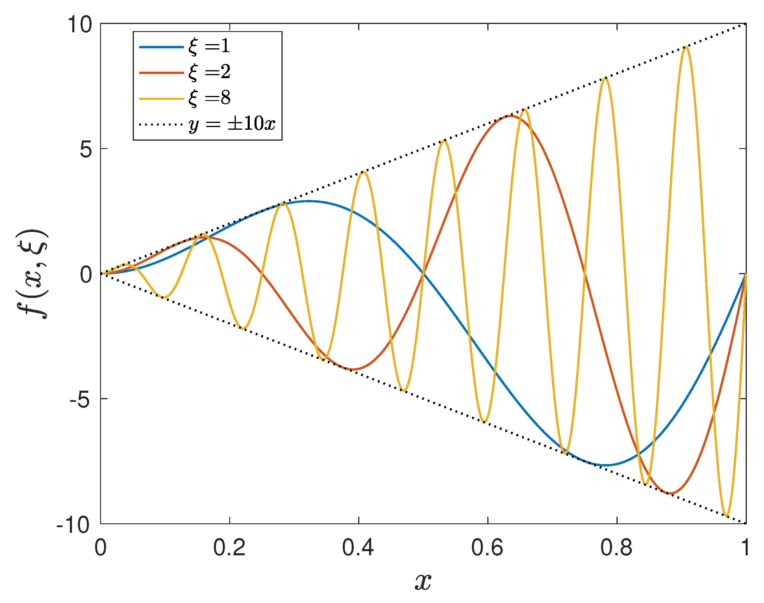
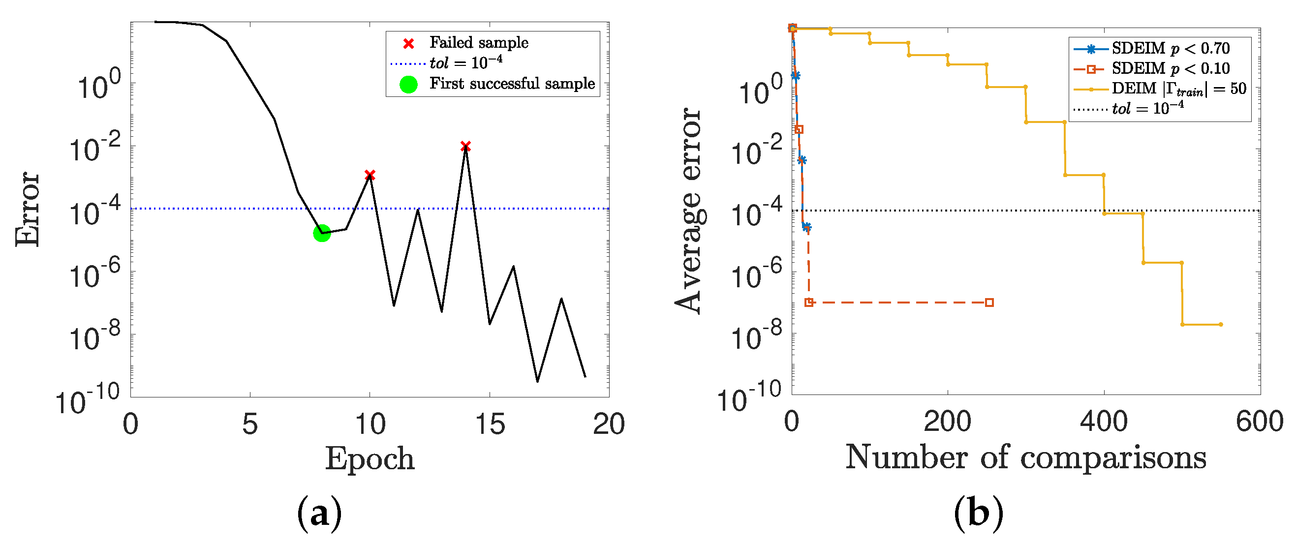
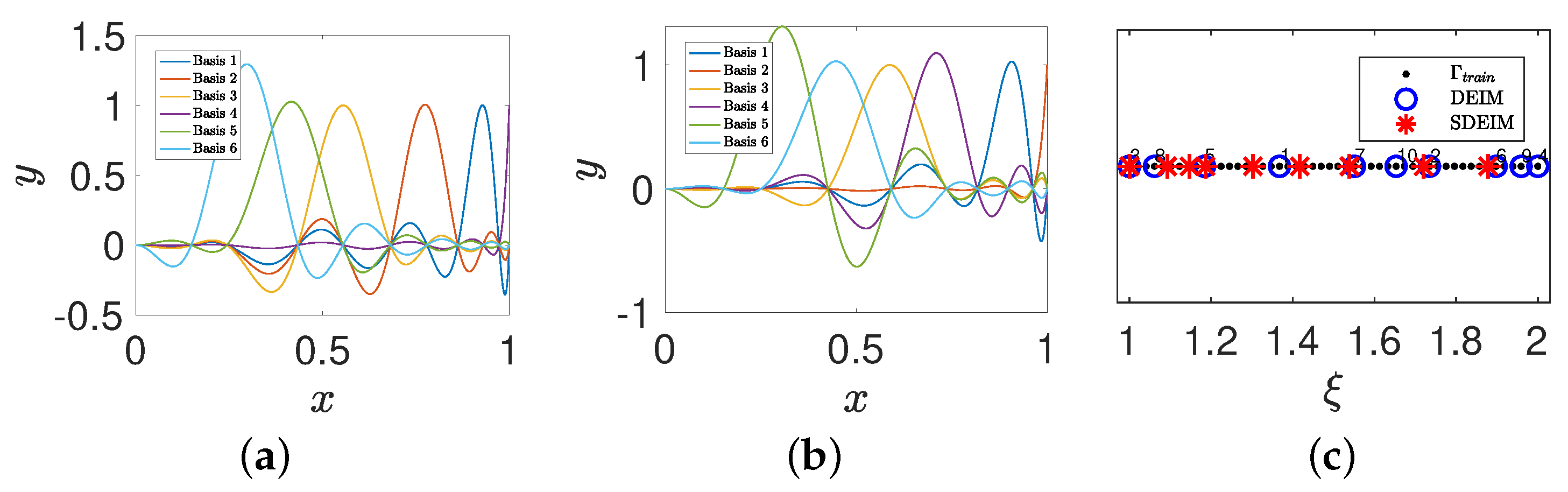
4.1. A Nonlinear Parameterized Function with Spatial Points in One Dimension

Consider a nonlinear parameterized function f : Ω × Γ R defined by
f ( x , ξ ) = 10 x sin 2 π ξ x ,
where x Ω = [ 0 , 1 ] R and ξ Γ = [ 1 , T ] R for a constant T. For a given parameter ξ , the function f ( x , ξ ) has the period 1 / ξ . Figure 1 plots the function f ( x , ξ ) for different ξ = 1 , 2 and 8. It shows that the target function can have different complexities for different parameter ranges. Let x ( i ) , i = 1 , 2 , , N h be a uniform grid points in Ω for N h = 400 , and define f h ( ξ ) : Γ R N h as
f h ( ξ ) = f x ( 1 ) , ξ , , f x ( N h ) , ξ T R N h
for ξ Γ . Let the range of the parameter be Γ = [ 1 , T ] for T = 2 and let Γ train be selected uniformly over Γ with | Γ train | = 50 for DEIM. The tolerance t o l is set to t o l = 10 4 and the confidence is set to 0.99 ( δ = 10 2 ) for Algorithms 1 and 2.
Figure 2 shows the training procedures for different methods. Figure 2a is the training procedure of SDEIM with threshold ε = 0.70 . An epoch in Figure 2a is a training procedure for a new realization ξ . The black curve indicates that the error changes in the training procedure. The green point is the first successful sample with η ( ξ ) t o l . In DEIM, after traversing the candidate sample set, if the sample with the largest error is less than tolerance t o l , the algorithm stops and the linear approximation space satisfies η ( ξ ) t o l for all ξ Γ train . In SDEIM, we continue to find whether there are failed samples (the red crosses) in Γ with η ( ξ ) > t o l . The SDEIM algorithm (Algorithm 2) stops when the samples satisfy η ( ξ ) t o l for N consecutive samples. In this case, the probability for the appearance of a failed sample is considered to be very low in SDEIM. Figure 2b shows the relationship between the number of comparisons and the average error in the training procedure for SDEIM (with p < 0.70 and p < 0.10 ) and DEIM, where the average error is computed on N ˜ = 10 4 samples defined as
η ¯ : = 1 N ˜ i = 1 N ˜ η ξ ( i ) .
Since a basis function is found after searching the candidate sample set Γ train in DEIM, its average error decreases in a ladder shape. In SDEIM, errors for an extra N consecutive samples need to be computed, and its numbers of comparisons have a long flat tail.
Table 1 shows more details for the linear approximation space V produced by the two methods. The average errors η ¯ for different methods are computed using (26) with N ˜ = 10 4 samples and the empirical probabilities p ¯ are calculated using (22) with the same N ˜ = 10 4 samples which are the approximation of p. The number of comparisons is the times in different methods to compare the error η ( ξ ) . From Table 1, it can be seen that since SDEIM does not need to search the sample ξ in a candidate sample set Γ train , it has fewer comparisons.
Figure 3a,b show the first six basis functions (i.e., the first six columns of matrix Q ˜ ) for DEIM and SDEIM. Figure 3c shows the samples ξ which generate the basis functions for DEIM and SDEIM. The black dots in Figure 3c are the samples in the candidate sample set Γ train , and the black dots circled by the blue circles are the samples selected by DEIM. The numbers above them are the order in which they are selected. The red stars are the samples selected by SDEIM, which are generated in random order. Note that the consecutive samples in DEIM are separated further because they are selected after searching the fine candidate sample set Γ train .

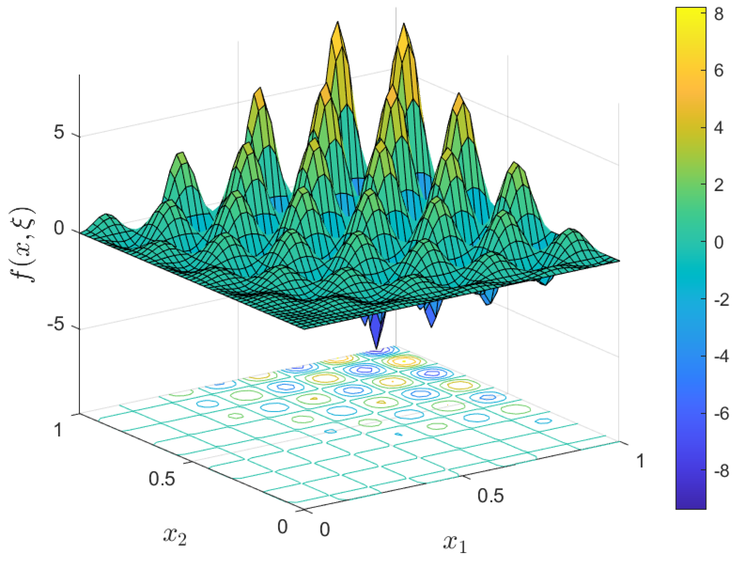
4.2. A Nonlinear Parameterized Function with Spatial Points in Two Dimensions

Consider a nonlinear parameterized function f : Ω × Γ R defined by
f ( x , ξ ) = 10 x 1 x 2 sin 2 π ξ 1 x 1 cos 2 π ξ 2 x 2 ,
where x = ( x 1 , x 2 ) Ω = [ 0 , 1 ] 2 R 2 and ξ = ( ξ 1 , ξ 2 ) Γ = [ 1 , T ] 2 R 2 for a constant T. Similarly to Section 4.1, for a large ξ 1 (or ξ 2 ), f ( x , ξ ) changes more quickly in the x 1 (or x 2 ) direction. Let x ( i ) , i = 1 , 2 , , N h be a uniform grid in Ω for N h = 50 × 50 = 2500 , and define f h ( ξ ) : Γ R N h as
f h ( ξ ) = f x ( 1 ) , ξ , , f x ( N h ) , ξ T R N h
for ξ Γ . Let the range of the parameter be Γ = [ 1 , T ] 2 for T = 4 . Figure 4 shows the image of f ( x , ξ ) for ξ = [ 4 , 4 ] . The tolerance t o l is set to t o l = 10 4 and the confidence is set to 0.99 for δ = 10 2 for Algorithms 1 and 2.
Figure 5 shows the training procedures for the two methods. Where Figure 5a is the training procedure of SDEIM with threshold ε = 0.10 . An epoch in Figure 5a is a comparison of the error for a new realization of ξ . The trend of black dots is the trend of errors, which decrease rapidly at early epochs. For these early epochs, the linear approximation space is updated for each realization ξ in this stage. After the first successful sample (the green point with η ( ξ ) t o l ), the error becomes relatively stable near the t o l . Then, for SDEIM, the linear approximation space is updated only for the failed samples (the red crosses with η ( ξ ) > t o l ), and Algorithm 2 stops when the samples satisfy η ( ξ ) t o l for N consecutive samples. Figure 5b shows the relationship between the number of comparisons and the average error among N ˜ = 10 4 samples in the training procedure for SDEIM and DEIM. Compared with DEIM, SDEIM has fewer comparisons.
Table 2 shows more details for DEIM and SDEIM with different parameters, where the average errors η ¯ and the empirical probability p ¯ for different parameters are computed using (22) and (26) on the same N ˜ = 10 4 samples. It can be seen that the empirical probability p ¯ for DEIM is similar to that of SDEIM. Moreover, by comparing DEIM with the size of candidate sample set | Γ train | = 400 and SDEIM with probability threshold ε = 0.10 , the number of comparisons for SDEIM is far less than DEIM.

4.3. Random Fields

Consider a nonlinear parameterized function f : Ω × Γ R defined by
f ( x , ξ ) = exp z ( x , ξ ) ,
where x = ( x 1 , x 2 ) Ω = [ 0 , 1 ] 2 R 2 and z ( x , ξ ) is assumed to be a stochastic process with mean function z 0 ( x ) 1 and covariance function Cov ( x , y ) defined as
Cov ( x , y ) = σ 2 exp | x 1 y 1 | L | x 2 y 2 | L .
Here x = ( x 1 , x 2 ) Ω , y = ( y 1 , y 2 ) Ω and L is the correlation length. The Karhu nen–Loève (KL) expansion (see [24,25] for details) gives a representation of z ( x , ξ ) as
z ( x , ξ ) = z 0 ( x ) + i = 1 λ i φ i ( x ) ξ i ,
where { φ i ( x ) , i = 1 , 2 , } are the orthonormal eigenfunctions and { λ i , i = 1 , 2 , } are the corresponding eigenvalues of the covariance function Cov ( x , y ) . Moreover, { ξ i , i = 1 , 2 , } are mutually uncorrelated random variables. In this example, we truncate the expansion to M terms as our surrogate model according the retaining of the energy for z ( x , ξ ) :
z M ( x , ξ ) : = z 0 ( x ) + i = 1 M λ i φ i ( x ) ξ i ,
where ξ = ( ξ 1 , , ξ M ) is the parameter in the surrogate model whose distribution is assumed to be a uniform distribution in Γ = [ 1 , 1 ] M R M and M satisfies
δ K L : = i = 1 M λ i | Ω | σ 2 > 0.95 .
Here, | Ω | is the area of the physical domain Ω and the standard deviation σ is set to σ = 0.5 for (27). We focus on the cases L = 1 and L = 0.5 in this experiment, and the corresponding dimensions of the parameter spaces are M = 33 and M = 109 respectively. The physical grid is set to a uniform grid with N h = 50 × 50 = 2500 . We consider the nonlinear parameterized function f h ( ξ ) : Γ R N h defined by
f h ( ξ ) = f M x ( 1 ) , ξ , , f M x ( N h ) , ξ T R N h
for ξ Γ , where f M ( x , ξ ) = exp ( z M ( x , ξ ) ) .
Figure 6a,b show the error for SDEIM with dimensions M = 33 and M = 109 for N ˜ = 10 3 samples respectively. The tolerance is set to t o l = 10 3 , the threshold is set to ε = 0.30 and the confidence is set to 0.99 for δ = 10 2 in Algorithm 2. Here the black points are the samples satisfying η ( ξ ) t o l and the red crosses are the failed samples satisfying η ( ξ ) > t o l . The empirical probabilities p ¯ are p ¯ = 0.062 and p ¯ = 0.051 , which are both smaller than our probability threshold ε = 0.30 .
Table 3 shows more details about the property of SDEIM in different parameter settings. The data in Table 3 are calculated with N ˜ = 10 4 samples and the data in Figure 6 are the first 10 3 of these 10 4 samples. From Table 3, it can be seen that for different dimensions of parameter spaces ( M = 33 and M = 109 ) and different tolerances ( t o l = 10 1 , 10 2 , 10 3 ), SDEIM can produce a linear approximation space V satisfying different probability thresholds ( ε = 0.70 , 0.50 , 0.30 , 0.10 ). Table 4 shows the average number of comparisons for each basis function in SDEIM with different parameter settings. The average number of comparisons is the ratio of the number of comparisons to the number of basis functions for the linear approximation space V . It is clear that SDEIM has a very small number of comparisons to generate each basis function.

4.4. The FitzHugh–Nagumo (F-N) System

This test problem considers the F-N system, which is a simplified model of spiking neuron activation and deactivation dynamics [6,16]. Within the F-N system, the nonlinear function f ( v ) is defined as
f ( v ) = v ( v 0.01 ) ( 1 v ) ,
where v is the voltage and satisfies the F-N system
ε v t ( x , t ) = ε 2 v x x ( x , t ) + f ( v ( x , t ) ) w ( x , t ) + c , w t ( x , t ) = b v ( x , t ) γ w ( x , t ) + c ,
with ε = 0.015 , b = 0.5 , γ = 2 , c = 0.05 and x Ω = [ 0 , L ] , t 0 . The variable w represents the recovery of voltage, and the variable L is set to L = 1 . Following the settings in [6], initial and boundary conditions are set to
v ( x , 0 ) = 0 , w ( x , 0 ) = 0 , x Ω = [ 0 , L ] , v x ( 0 , t ) = i 0 ( t ) , v x ( L , t ) = 0 , t 0 ,
where the stimulus i 0 ( t ) = 50 , 000 t 3 exp ( 15 t ) . We discretize the physical domain Ω using a uniform grid with N h = 2500 . The dimension of the finite difference system is 2500. We take 2501 time nodes at evenly in the interval [ 0 , 8 ] , of which 500 are randomly selected as the candidate sample set Γ train for DEIM and SDEIM training, and the remainder are utilized to test the probability features.
The solution of the F-N system has a limit cycle for each spatial variable x, and we display the phase-space diagram of v and w at various spatial positions in Figure 7. Symmetry in the limit cycles of the F-N system is well captured by SDEIM, as seen in Figure 7. Tolerances are set to t o l = 10 3 for solutions v , w and t o l = 10 4 for nonlinear function f ( v ) . The probability of errors exceeding the corresponding tolerances among 1500 verifying samples are depicted in Figure 8a. The probabilities of v converge to a constant value in this case, because the accuracy of the solution v is dependent on the accuracy of the solution w for both DEIM and SDEIM. Figure 8b shows the number of comparisons increases as the number of basis functions increases. The black dotted line represents the number of comparisons in DEIM, which is ( 2 | Γ train | n + 1 ) n / 2 (n is the number of the basis functions). It is clear that SDEIM is very efficient solve this F-N system.

5. Conclusions

Empirical interpolation is a widely used model reduction method for nonlinear and nonaffine parameterized systems through a separate representation of the spatial and the parametric variables. This kind of method typically requires a fine candidate sample set, which can lead to high computational costs. With a focus on randomized computational methods, we in this paper propose a stochastic discrete empirical interpolation method (SDEIM). In SDEIM, large candidate sample sets are replaced by gradually generated random samples, such that the computational costs of constructing the corresponding interpolation formulation can be dramatically reduced. With our analysis, the stopping criterion based on a probability threshold in SDEIM can guarantee the interpolation is accurate with a given confidence. Our numerical results show that this randomized approach is efficient, especially for variable separation for high dimensional nonlinear and nonaffine systems. However, as we use the Hoeffding’s inequality to estimate the failure probability in the verifying stage, SDEIM is efficient when this probability is not too small, but it can be inefficient when the probability is very small. For applying SDEIM to systems which require high reliability, current efforts are focused on combining subset simulation methods, and implementing such strategies will be the focus of our future work.

Author Contributions

Conceptualization, D.C. and Q.L.; methodology, D.C. and Q.L.; software, D.C. and C.Y.; validation, D.C.; writing—original draft preparation, D.C. and C.Y.; writing—review and editing, D.C. and Q.L.; supervision, Q.L.; project administration, Q.L.; funding acquisition, Q.L. All authors have read and agreed to the published version of the manuscript.

Funding

This work is supported by the Science and Technology Commission of Shanghai Municipality (No. 20JC1414300) and the Natural Science Foundation of Shanghai (No. 20ZR1436200).

Institutional Review Board Statement

Not applicable.

Informed Consent Statement

Not applicable.

Data Availability Statement

Not applicable.

Conflicts of Interest

The authors declare no conflict of interest.

References

  1. Benner, P.; Gugercin, S.; Willcox, K. A survey of projection-based model reduction methods for parametric dynamical systems. SIAM Rev. 2015, 57, 483–531. [Google Scholar] [CrossRef]
  2. Barrault, M.; Maday, Y.; Nguyen, N.C.; Patera, A.T. An ‘empirical interpolation’ method: Application to efficient reduced-basis discretization of partial differential equations. C. R. Math. 2004, 339, 667–672. [Google Scholar] [CrossRef]
  3. Maday, Y.; Mula, O. A generalized empirical interpolation method: Application of reduced basis techniques to data assimilation. In Analysis and Numerics of Partial Differential Equations; Springer: Berlin/Heidelberg, Germany, 2013; pp. 221–235. [Google Scholar]
  4. Chen, P.; Quarteroni, A.; Rozza, G. A weighted empirical interpolation method: A priori convergence analysis and applications. ESAIM Math. Model. Numer. Anal. 2014, 48, 943–953. [Google Scholar] [CrossRef] [Green Version]
  5. Elman, H.C.; Forstall, V. Numerical solution of the parameterized steady-state Navier–Stokes equations using empirical interpolation methods. Comput. Methods Appl. Mech. Eng. 2017, 317, 380–399. [Google Scholar] [CrossRef] [Green Version]
  6. Chaturantabut, S.; Sorensen, D.C. Nonlinear model reduction via discrete empirical interpolation. SIAM J. Sci. Comput. 2010, 32, 2737–2764. [Google Scholar] [CrossRef]
  7. Peherstorfer, B.; Butnaru, D.; Willcox, K.; Bungartz, H.J. Localized discrete empirical interpolation method. SIAM J. Sci. Comput. 2014, 36, A168–A192. [Google Scholar] [CrossRef]
  8. Li, Q.; Jiang, L. A novel variable-separation method based on sparse and low rank representation for stochastic partial differential equations. SIAM J. Sci. Comput. 2017, 39, A2879–A2910. [Google Scholar] [CrossRef]
  9. Veroy, K.; Rovas, D.V.; Patera, A.T. A posteriori error estimation for reduced-basis approximation of parametrized elliptic coercive partial differential equations: “Convex inverse” bound conditioners. ESAIM Control. Optim. Calc. Var. 2002, 8, 1007–1028. [Google Scholar] [CrossRef] [Green Version]
  10. Quarteroni, A.; Rozza, G. Numerical solution of parametrized Navier–Stokes equations by reduced basis methods. Numer. Methods Partial Differ. Equ. Int. J. 2007, 23, 923–948. [Google Scholar] [CrossRef]
  11. Chen, P.; Quarteroni, A.; Rozza, G. Comparison between reduced basis and stochastic collocation methods for elliptic problems. J. Sci. Comput. 2014, 59, 187–216. [Google Scholar] [CrossRef]
  12. Jiang, J.; Chen, Y.; Narayan, A. A goal-oriented reduced basis methods-accelerated generalized polynomial chaos algorithm. SIAM/ASA J. Uncertain. Quantif. 2016, 4, 1398–1420. [Google Scholar] [CrossRef]
  13. Elman, H.C.; Liao, Q. Reduced basis collocation methods for partial differential equations with random coefficients. SIAM/ASA J. Uncertain. Quantif. 2013, 1, 192–217. [Google Scholar] [CrossRef] [Green Version]
  14. Liao, Q.; Lin, G. Reduced basis ANOVA methods for partial differential equations with high-dimensional random inputs. J. Comput. Phys. 2016, 317, 148–164. [Google Scholar] [CrossRef] [Green Version]
  15. Cohen, A.; Dahmen, W.; DeVore, R.; Nichols, J. Reduced basis greedy selection using random training sets. ESAIM Math. Model. Numer. Anal. 2020, 54, 1509–1524. [Google Scholar] [CrossRef] [Green Version]
  16. Rocsoreanu, C.; Georgescu, A.; Giurgiteanu, N. The FitzHugh–Nagumo Model: Bifurcation and Dynamics; Springer Science & Business Media: Berlin/Heidelberg, Germany, 2012; Volume 10. [Google Scholar]
  17. Grepl, M.A.; Maday, Y.; Nguyen, N.C.; Patera, A.T. Efficient reduced-basis treatment of nonaffine and nonlinear partial differential equations. ESAIM Math. Model. Numer. Anal. 2007, 41, 575–605. [Google Scholar] [CrossRef] [Green Version]
  18. Maday, Y.; Stamm, B. Locally adaptive greedy approximations for anisotropic parameter reduced basis spaces. SIAM J. Sci. Comput. 2013, 35, A2417–A2441. [Google Scholar] [CrossRef] [Green Version]
  19. Temlyakov, V.N. Nonlinear Kolmogorov widths. Math. Notes 1998, 63, 785–795. [Google Scholar] [CrossRef]
  20. Cuong, N.N.; Veroy, K.; Patera, A.T. Certified real-time solution of parametrized partial differential equations. In Handbook of Materials Modeling; Springer: Berlin/Heidelberg, Germany, 2005; pp. 1529–1564. [Google Scholar]
  21. Kristoffersen, S. The Empirical Interpolation Method. Master’s Thesis, Institutt for Matematiske Fag, Trondheim, Norway, 2013. [Google Scholar]
  22. Dudley, R.M. Real Analysis and Probability; CRC Press: Boca Raton, FL, USA, 2018. [Google Scholar]
  23. Hoeffding, W. Probability inequalities for sums of bounded random variables. In The Collected Works of Wassily Hoeffding; Springer: Berlin/Heidelberg, Germany, 1994; pp. 409–426. [Google Scholar]
  24. Ghanem, R.G.; Spanos, P.D. Stochastic Finite Elements: A Spectral Approach; Courier Corporation: Chelmsford, MA, USA, 2003. [Google Scholar]
  25. Lord, G.J.; Powell, C.E.; Shardlow, T. An Introduction to Computational Stochastic PDEs; Cambridge University Press: Cambridge, UK, 2014; Volume 50. [Google Scholar]
Figure 1. The parameterized function f ( x , ξ ) for ξ = 1 , 2 and 8.
Symmetry 14 00556 g001
Figure 2. (a) The training procedure of SDEIM with probability threshold ε = 0.70 , i.e., p < 0.70 , where each epoch is to test a new sample ξ for updating the basis. (b) The relationship between the number of comparisons and the average error in the training procedure for SDEIM (with p < 0.70 and p < 0.10 ) and DEIM.
Symmetry 14 00556 g002
Figure 3. (a) The first six basis functions for DEIM. (b) The first six basis functions for SDEIM. (c) The samples for generating the basis functions.
Symmetry 14 00556 g003
Figure 4. The parameterized function f ( x , ξ ) for ξ = [ 4 , 4 ] .
Symmetry 14 00556 g004
Figure 5. (a) The training procedure of SDEIM with probability threshold ε = 0.10 , i.e., p < 0.10 , where each epoch is to test a new sample ξ for updating the basis. (b) The relationship between the number of comparisons and the average error in the training procedure for DEIM and SDEIM with different parameters.
Symmetry 14 00556 g005
Figure 6. (a) The error for SDEIM with M = 33 . (b) The error for SDEIM with M = 109 . Each point or fork corresponds to a sample of the parameter.
Symmetry 14 00556 g006
Figure 7. (a) Phase-space diagram of v and w at different spatial points x from the FD system ( d i m 2500 ), DEIM reduced system ( d i m 67 ) and SDEIM reduced system ( d i m 72 ). (b) Corresponding projection of the solution onto the v w plane.
Symmetry 14 00556 g007
Figure 8. (a) Probability properties for DEIM reduced system and SDEIM reduced system. (b) The number of comparisons for DEIM reduced system and SDEIM reduced system.
Symmetry 14 00556 g008
Table 1. The average error η ¯ , the number of basis functions n for the approximation space V , the empirical probability p ¯ and the number of comparisons for SDEIM (with p < 0.70 and p < 0.10 ) and DEIM (with | Γ train | = 50 ).
η ¯ n p ¯ Number of Comparisons
SDEIM p < 0.70 2.8815 × 10 5 9 7.36 × 10 2 14 + N ( N = 5 )
p < 0.10 1.0145 × 10 7 100 22 + N ( N = 231 )
DEIM | Γ train | = 50 1.9514 × 10 8 100550
Table 2. The average error η ¯ , the number of basis functions n for the approximation space V , the empirical probability p ¯ and the number of comparisons for SDEIM with ( p < 0.70 and p < 0.10 ) and DEIM with ( | Γ train | = 225 and | Γ train | = 400 ).
η ¯ n p ¯ Number of Comparisons
SDEIM p < 0.70 3.7000 × 10 3 173 2.631 × 10 1 186 + N ( N = 5 )
p < 0.10 4.0844 × 10 6 204 2.500 × 10 3 869 + N ( N = 231 )
DEIM | Γ train | = 225 1.1881 × 10 4 177 1.876 × 10 1 40,050
| Γ train | = 400 2.1180 × 10 5 184 2.520 × 10 2 74,000
Table 3. The empirical probability p ¯ for different parameter settings in SDEIM.
ε = 0.70 ε = 0.50 ε = 0.30 ε = 0.10
N = 5 N = 10 N = 26 N = 231
M = 33 t o l = 10 1 3.060 × 10 1 2.189 × 10 1 4.770 × 10 2 2.700 × 10 3
t o l = 10 2 2.766 × 10 1 1.550 × 10 1 6.420 × 10 2 6.700 × 10 3
t o l = 10 3 5.344 × 10 1 2.406 × 10 1 5.550 × 10 2 1.890 × 10 2
M = 109 t o l = 10 1 5.664 × 10 1 2.567 × 10 1 1.173 × 10 1 1.050 × 10 2
t o l = 10 2 4.233 × 10 1 2.143 × 10 1 4.740 × 10 2 9.900 × 10 3
t o l = 10 3 1.863 × 10 1 1.403 × 10 1 5.020 × 10 2 4.400 × 10 3
Table 4. The average number of comparisons for each basis function in SDEIM with different parameter settings.
ε = 0.70 ε = 0.50 ε = 0.30 ε = 0.10
M = 33 t o l = 10 1 1.1037 1.1841 1.7954 5.4669
t o l = 10 2 1.0612 1.1284 1.3482 2.8485
t o l = 10 3 1.0346 1.1065 1.5488 2.5069
M = 109 t o l = 10 1 1.0372 1.1270 1.2069 2.6813
t o l = 10 2 1.0172 1.0527 1.1066 1.8194
t o l = 10 3 1.0291 1.0446 1.1196 2.2821
Publisher’s Note: MDPI stays neutral with regard to jurisdictional claims in published maps and institutional affiliations.

