
Scaled Three-Term Conjugate Gradient Methods for Solving Monotone Equations with Application


Abstract
:1. Introduction
2. The Scaled Three-Term CG Method
| Algorithm 1 Scaled Three-term CG method (STCG) |
| Step 0 Initialize: , , , , , and . Set and . |
| Step 1 If , stop, else go to Step 2. |
| Step 2 Compute the search direction using (7) and (11). |
| Step 3 Set and determine the step-length satisfying
|
| Step 4 If and stop, otherwise
|
| Step 5 Set and then go to Step 1. |
3. Analysis of the Global Convergence
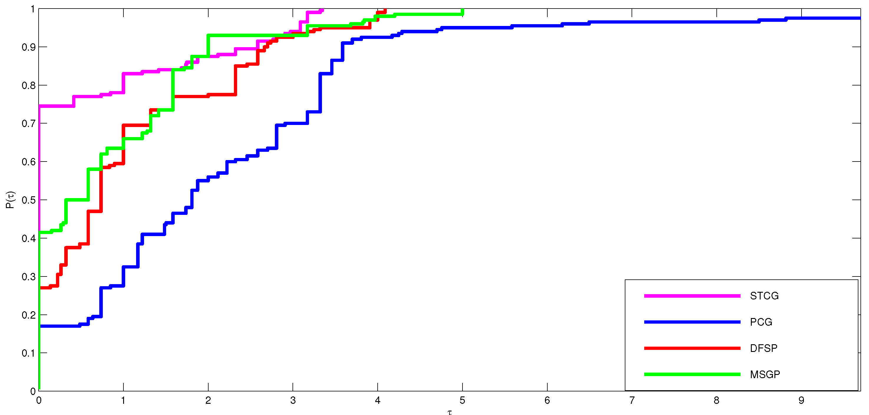
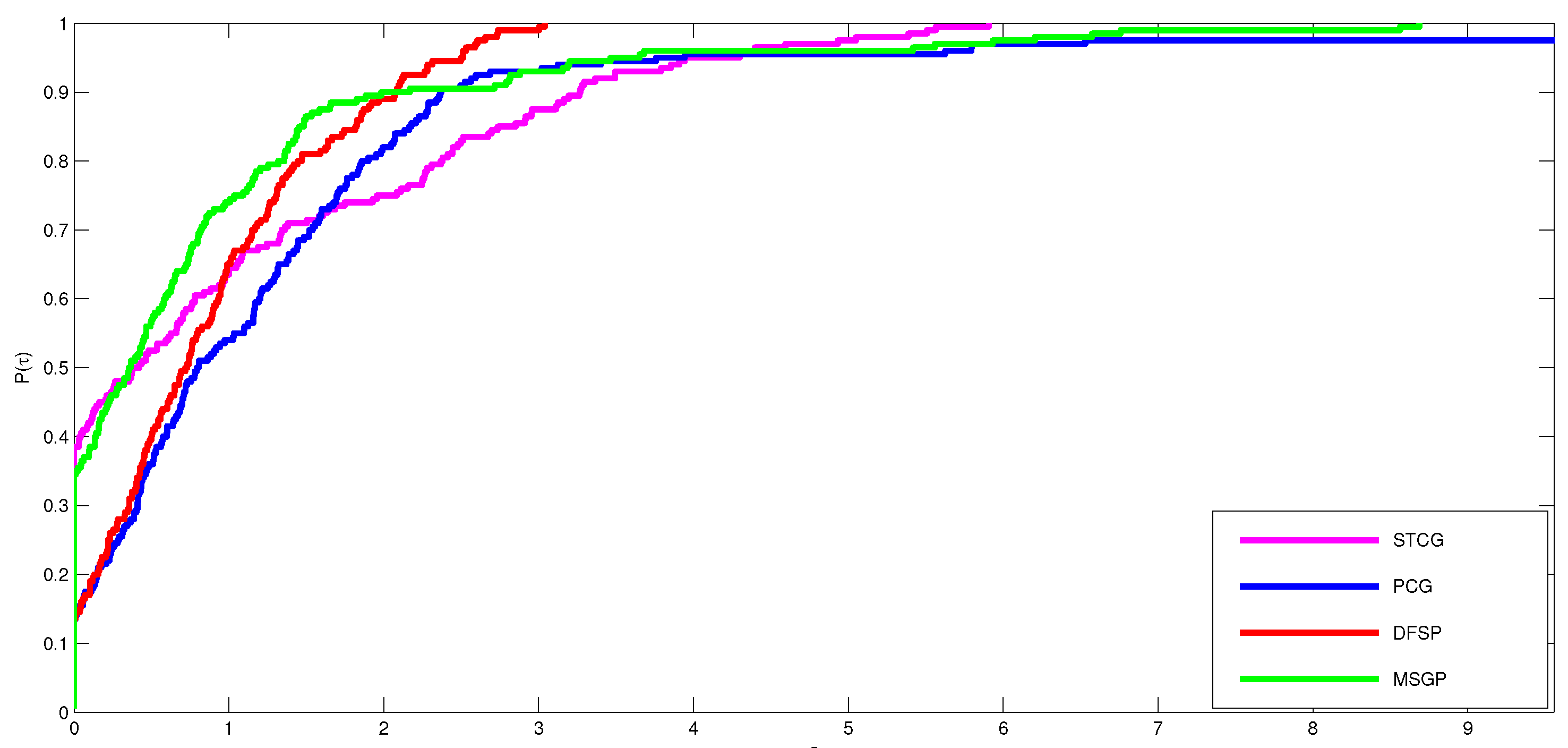
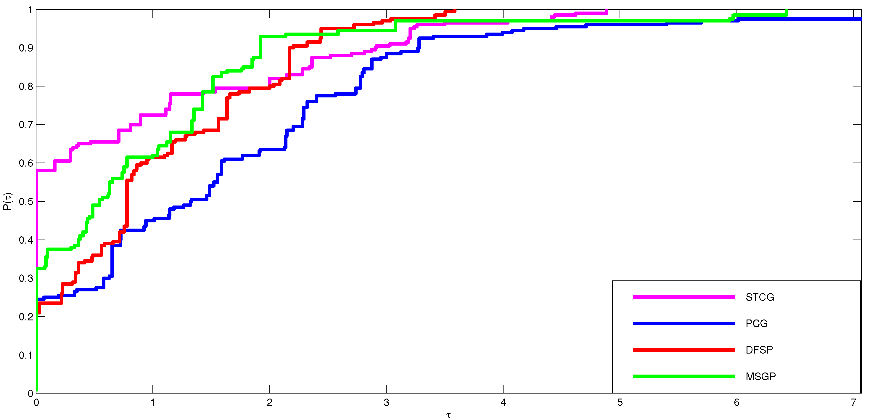
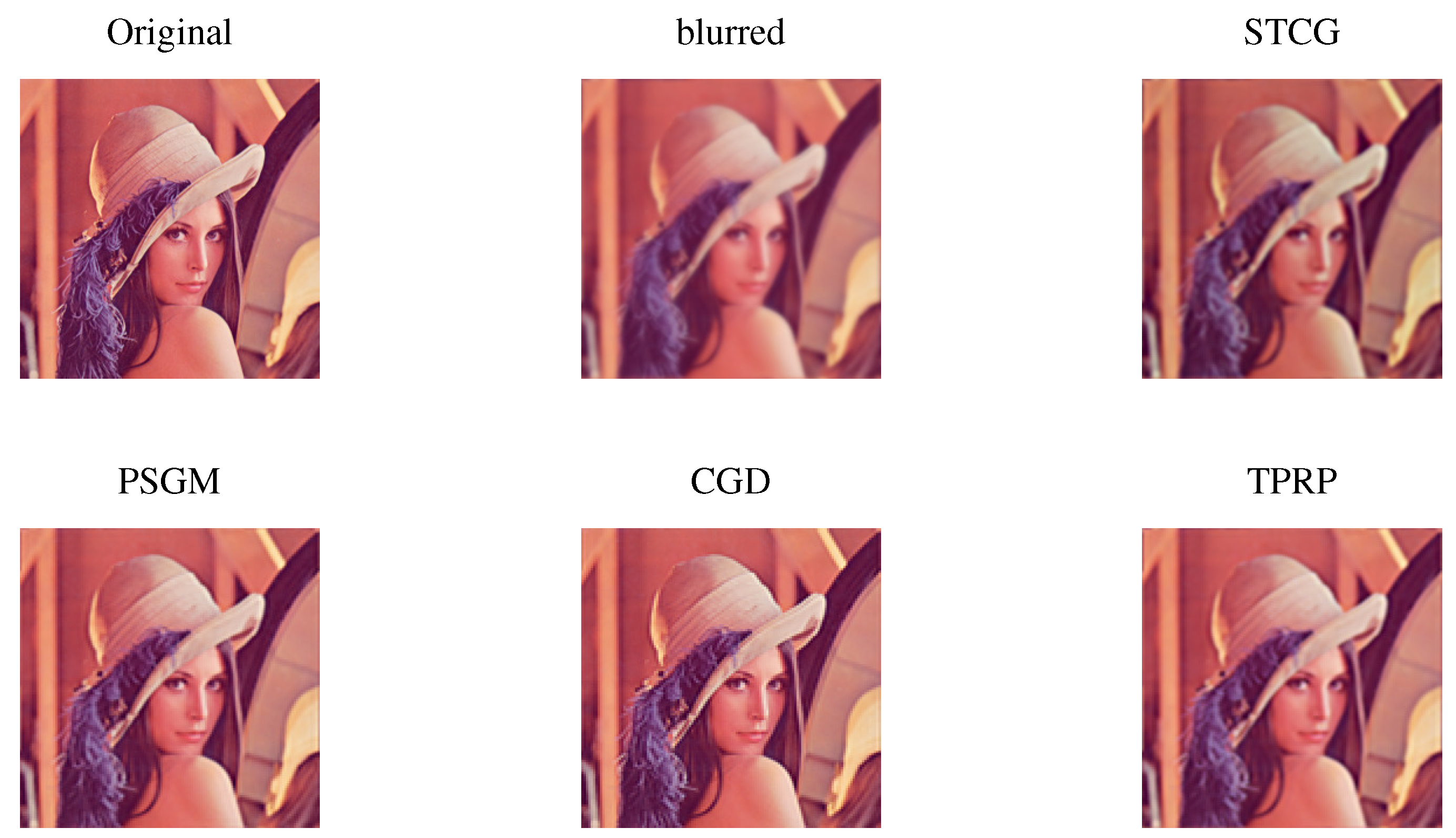
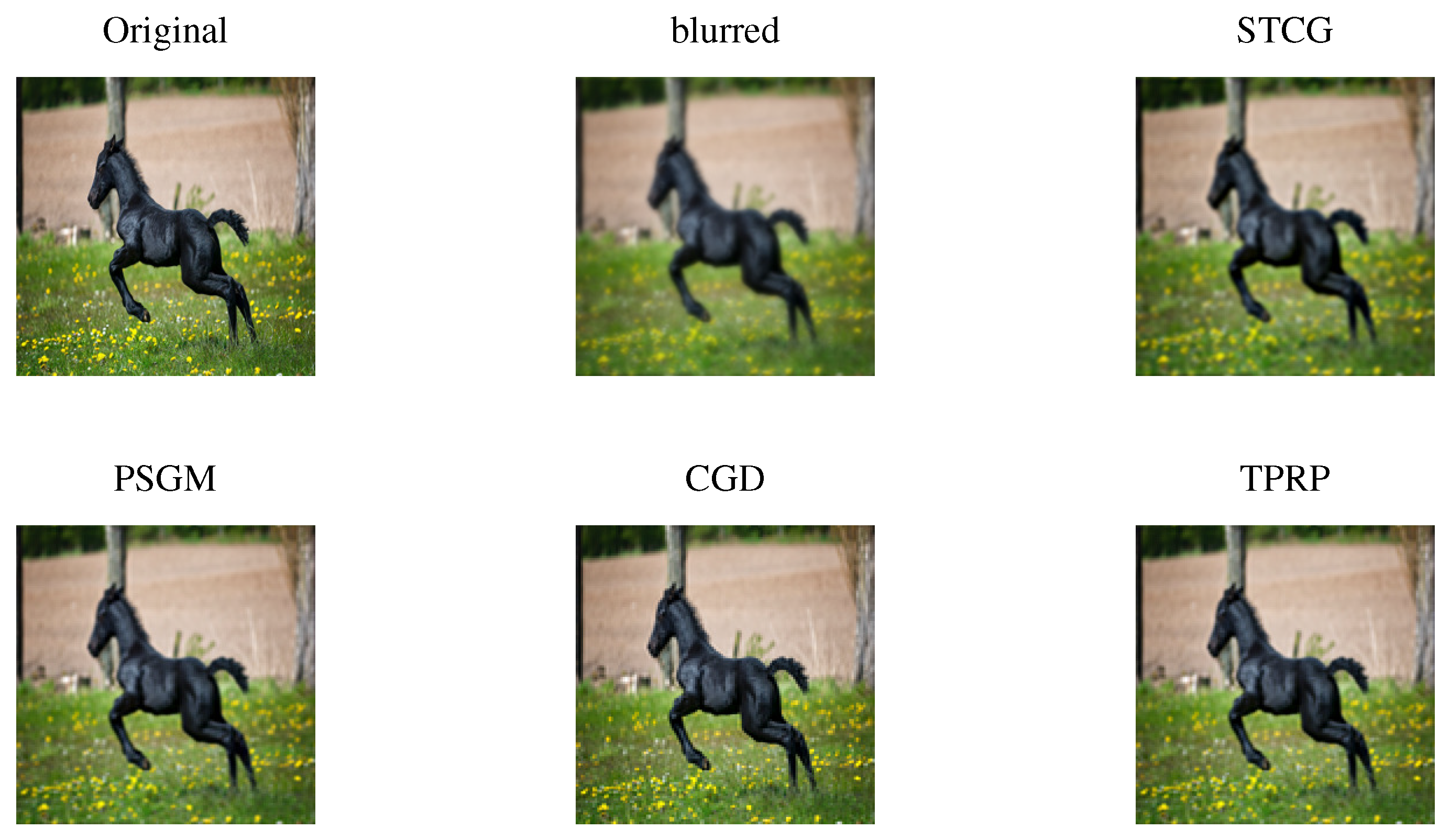
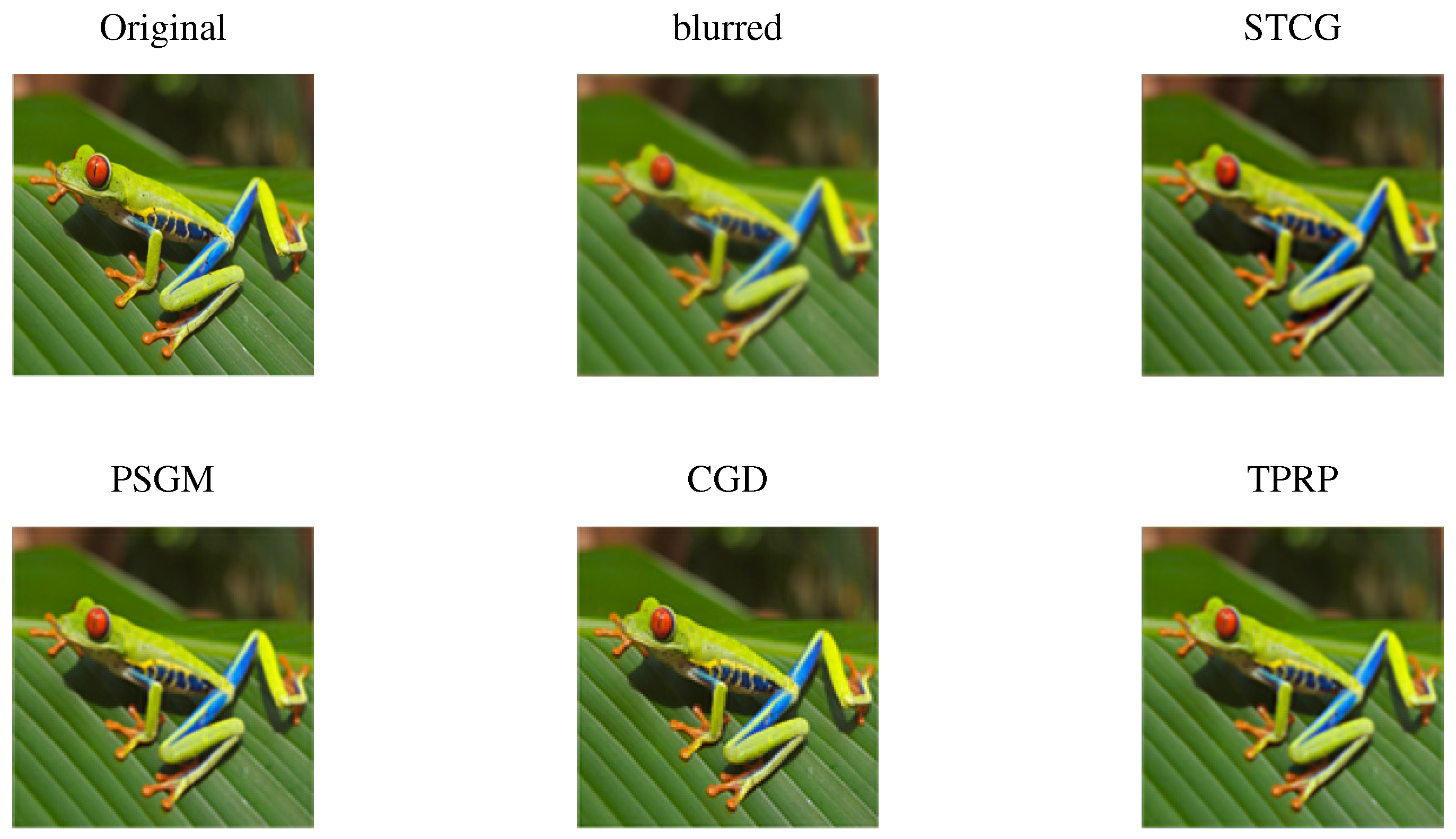
4. Numerical Experiment and Applications
4.1. Application to the Monotone Nonlinear Equations
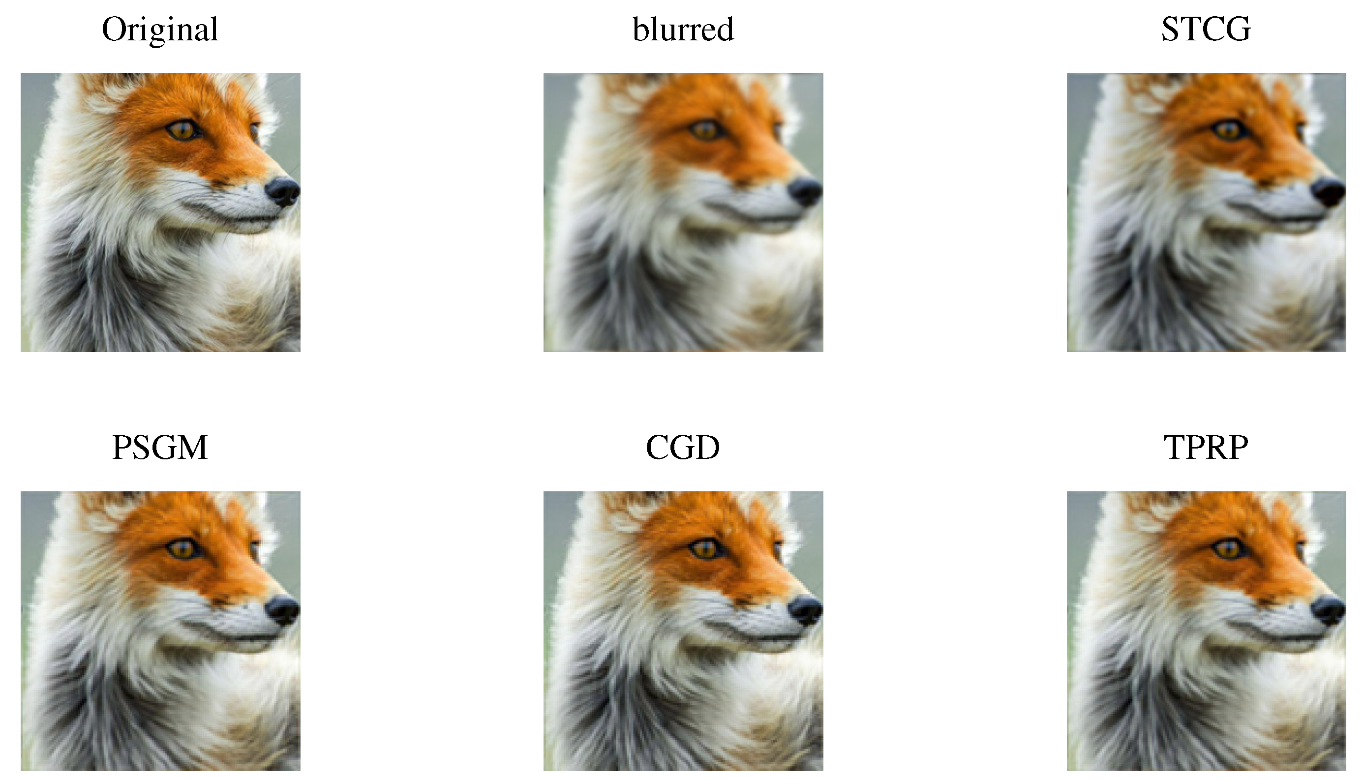
4.2. Application in Signal Recovery
5. Conclusions
Author Contributions
Funding
Institutional Review Board Statement
Informed Consent Statement
Data Availability Statement
Acknowledgments
Conflicts of Interest
References
- Iusem, A.N.; Solodov, M.V. Newton-type methods with generalized distances for constrained optimization. Optimization 1997, 41, 257–278. [Google Scholar] [CrossRef]
- Dai, Z.; Zhou, H.; Wen, F.; He, S. Efficient predictability of stock return volatility: The role of stock market implied volatility. N. Am. J. Econ. Financ. 2020, 52, 101174. [Google Scholar] [CrossRef]
- Figueiredo, M.; Nowak, R.; Wright, S.J. Gradient projection for sparse reconstruction, application to compressed sensing and other inverse problems. IEEE J. Sel. Top. Signal Process. 2007, 1, 586–597. [Google Scholar] [CrossRef] [Green Version]
- Zhao, Y.B.; Li, D.H. Monotonicity of fixed point and normal mapping associated with variational inequality and its application. SIAM J. Optim. 2001, 4, 962–973. [Google Scholar] [CrossRef]
- Li, D.; Fukushima, M. A Globally and Superlinearly Convergent Gauss-Newton-Based BFGS Method for Symmetric Nonlinear Equations. SIAM J. Numer. Anal. 1999, 37, 152–172. [Google Scholar] [CrossRef]
- Waziri, M.Y.; Sabi’u, J. A derivative-free conjugate gradient method and its global convergence for solving symmetric nonlinear equations. Int. J. Math. Math. Sci. 2015, 2015, 961487. [Google Scholar] [CrossRef] [Green Version]
- Sabi’u, J.; Muangchoo, K.; Shah, A.; Abubakar, A.B.; Aremu, K.O. An inexact optimal hybrid conjugate gradient method for solving symmetric nonlinear equations. Symmetry 2021, 13, 1829. [Google Scholar] [CrossRef]
- Sabi’u, J.; Muangchoo, K.; Shah, A.; Abubakar, A.B.; Jolaoso, L.O. A modified PRP-CG type derivative-free algorithm with optimal choices for solving large-scale nonlinear symmetric equations. Symmetry 2021, 13, 234. [Google Scholar] [CrossRef]
- Ortega, J.M.; Rheinboldt, W.C. Iterative Solution of Nonlinear Equations in Several Variables; Academic Press: Cambridge, MA, USA, 1970. [Google Scholar]
- Zhou, G.; Toh, K.C. Superlinear convergence of a Newton-type algorithm for monotone equations. J. Optimiz. Theory Appl. 2005, 125, 205–221. [Google Scholar] [CrossRef]
- Zhou, W.J.; Li, D.H. A globally convergent BFGS method for nonlinear monotone equations without any merit functions. Math. Comput. 2008, 77, 2231–2240. [Google Scholar] [CrossRef]
- Sabi’u, J.; Shah, A.; Waziri, M.Y.; Ahmed, K. Modified Hager-Zhang conjugate gradient methods via singular value analysis for solving monotone nonlinear equations with convex constraint. Int. J. Comput. Methods 2020, 18, 2050043. [Google Scholar] [CrossRef]
- Sabi’u, J.; Shah, A.; Waziri, M.Y. A modified Hager-Zhang conjugate gradient method with optimal choices for solving monotone nonlinear equations. Int. J. Comput. Math. 2022, 99, 332–354. [Google Scholar] [CrossRef]
- Sabi’u, J.; Shah, A. An efficient three-term conjugate gradient-type algorithm for monotone nonlinear equations. RAIRO Oper. Res. 2021, 55, S1113–S1127. [Google Scholar] [CrossRef]
- Waziri, M.Y.; Ahmed, K.; Sabi’u, J.; Halilu, A.S. Enhanced Dai–Liao conjugate gradient methods for systems of monotone nonlinear equations. SeMA J. 2021, 78, 15–51. [Google Scholar] [CrossRef]
- Abubakar, A.B.; Sabi’u, J.; Kumam, P.; Shah, A. Solving nonlinear monotone operator equations via modified sr1 update. J. Appl .Math. Comput. 2021, 67, 343–373. [Google Scholar] [CrossRef]
- Waziri, M.Y.; Hungu, K.A.; Sabi’u, J. Descent Perry conjugate gradient methods for systems of monotone nonlinear equations. Numer. Algorithms 2020, 85, 763–785. [Google Scholar] [CrossRef]
- Waziri, M.Y.; Ahmed, K.; Sabi’u, J. A Dai–Liao conjugate gradient method via modified secant equation for system of nonlinear equations. Arab. J. Math. 2020, 9, 443–457. [Google Scholar] [CrossRef] [Green Version]
- Sabi’u, J.; Shah, A.; Waziri, M.Y. Two optimal Hager-Zhang conjugate gradient methods for solving monotone nonlinear equations. Appl. Numer. Math. 2020, 153, 217–233. [Google Scholar] [CrossRef]
- Gao, P.; He, C. An efficient three-term conjugate gradient method for nonlinear monotone equations with convex constraints. Calcolo 2018, 55, 1–17. [Google Scholar] [CrossRef]
- Liu, J.; Feng, Y. A derivative-free iterative method for nonlinear monotone equations with convex constraints. Numer. Algorithms 2019, 82, 245–262. [Google Scholar] [CrossRef]
- Zheng, L.; Yang, L.; Liang, Y. A modified spectral gradient projection method for solving non-linear monotone equations with convex constraints and its application. IEEE Access 2020, 8, 92677–92686. [Google Scholar] [CrossRef]
- Halilu, A.S.; Majumder, A.; Waziri, M.Y.; Ahmed, K. Signal recovery with convex constrained nonlinear monotone equations through conjugate gradient hybrid approach. Math. Comput. Simul. 2021, 187, 520–539. [Google Scholar] [CrossRef]
- Koorapetse, M.; Kaelo, P.; Lekoko, S.; Diphofu, T. A derivative-free RMIL conjugate gradient projection method for convex constrained nonlinear monotone equations with applications in compressive sensing. Appl. Numer. Math. 2021, 165, 431–441. [Google Scholar] [CrossRef]
- Halilu, A.S.; Majumder, A.; Waziri, M.Y.; Awwal, A.M.; Ahmed, K. On solving double direction methods for convex constrained monotone nonlinear equations with image restoration. Comput. Appl. Math. 2021, 40, 1–27. [Google Scholar] [CrossRef]
- Aji, S.; Kumam, P.; Awwal, A.M.; Yahaya, M.M.; Kumam, W. Two hybrid spectral methods with inertial effect for solving system of nonlinear monotone equations with application in robotics. IEEE Access 2021, 9, 30918–30928. [Google Scholar] [CrossRef]
- Amini, K.; Faramarzi, P.; Bahrami, S. A spectral conjugate gradient projection algorithm to solve the large-scale system of monotone nonlinear equations with application to compressed sensing. Int. J. Comput. Math. 2022, 2047180. [Google Scholar] [CrossRef]
- Waziri, M.Y.; Ahmed, K.; Halilu, A.S. A modified PRP-type conjugate gradient projection algorithm for solving large-scale monotone nonlinear equations with convex constraint. J. Comput. Appl. Math. 2022, 406, 114035. [Google Scholar] [CrossRef]
- Waziri, M.Y.; Ahmed, K. Two Descent Dai-Yuan Conjugate Gradient Methods for Systems of Monotone Nonlinear Equations. J. Sci. Comput. 2022, 90, 1–53. [Google Scholar] [CrossRef]
- Waziri, M.Y.; Ahmed, K.; Halilu, A.S.; Sabi’u, J. Two new Hager–Zhang iterative schemes with improved parameter choices for monotone nonlinear systems and their applications in compressed sensing. RAIRO Oper. Res. 2022, 56, 239–273. [Google Scholar] [CrossRef]
- Meli, E.; Morini, B.; Porcelli, M.; Sgattoni, C. Solving nonlinear systems of equations via spectral residual methods: Stepsize selection and applications. J. Sci. Comput. 2022, 90, 1–41. [Google Scholar] [CrossRef]
- Narushima, Y.; Yabe, H.; Ford, J.A. A three-term conjugate gradient method with sufficient descent property for unconstrained optimization. SIAM J. Optim. 2011, 21, 212–230. [Google Scholar] [CrossRef] [Green Version]
- Birgin, E.; Martinez, J.M. A spectral conjugate gradient method for unconstrained optimization. Appl. Math. Optim. 2001, 43, 117–128. [Google Scholar] [CrossRef] [Green Version]
- Liu, J.K.; Lia, S.J. A projection method for convex constrained monotone nonlinear equations with applications. Comput. Math. Appl. 2015, 70, 2442–2453. [Google Scholar] [CrossRef]
- La Cruz, W.; Martinez, J.; Raydan, M. Spectral residual method without gradient information for solving large-scale nonlinear systems of equations. Math. Comput. 2006, 75, 1429–1448. [Google Scholar] [CrossRef] [Green Version]
- Hu, Y.; Wei, Z. A modified Liu-Storey conjugate gradient projection algorithm for nonlinear monotone equations. Int. Math. Forum. 2014, 9, 1767–1777. [Google Scholar] [CrossRef] [Green Version]
- Dolan, E.D.; More, J.J. Benchmarking optimization software with performance profiles. Math. Program. 2002, 91, 201–213. [Google Scholar] [CrossRef]
- Hale, E.T.; Yin, W.; Zhang, Y. A fixed-point continuation method for l1 regularized minimization with applications to compressed sensing. SIAM J. Optim. 2008, 19, 1107–1130. [Google Scholar] [CrossRef]
- Beck, A.; Teboulle, M. A fast iterative shrinkage-thresholding algorithm for linear inverse problems. SIAM J. Imaging Sci. 2009, 2, 183–202. [Google Scholar] [CrossRef] [Green Version]
- Van den Berg, E.; Friedlander, M.P. Probing the pareto frontier for basis pursuit solutions. SIAM J. Sci. Comput. 2008, 31, 890–912. [Google Scholar] [CrossRef] [Green Version]
- Xiao, Y.H.; Wang, Q.Y.; Hu, Q.J. Non-smooth equations based method for l1-norm problems with applications to compressed sensing. Nonlinear Anal. Theory Methods Appl. 2011, 74, 3570–3577. [Google Scholar] [CrossRef]
- Pang, J.S. Inexact Newton methods for the nonlinear complementarity problem. Math. Program. 1986, 36, 54–71. [Google Scholar] [CrossRef]
- Awwal, A.M.; Kumam, P.; Mohammad, H.; Watthayu, W.; Abubakar, A.B. A Perry-type derivative-free algorithm for solving nonlinear system of equations and minimizing l1 regularized problem. Optimization 2021, 70, 1231–1259. [Google Scholar] [CrossRef]
- Xiao, Y.H.; Zhu, H. A conjugate gradient method to solve convex constrained monotone equations with applications in compressive sensing. J. Math. Anal. 2013, 405, 310–319. [Google Scholar] [CrossRef]
- Ibrahim, A.H.; Deepho, J.; Abubakar, A.B.; Adamu, A. A three-term Polak-Ribiére-Polyak derivative-free method and its application to image restoration. Sci. Afr. 2021, 13, e00880. [Google Scholar]


| Problem 1 | STCG | PCG | DFSP | MSGP | |||||||||||||
|---|---|---|---|---|---|---|---|---|---|---|---|---|---|---|---|---|---|
| DIMENSION | >INITIAL POINT | ITER | FVAL | TIME | NORM | ITER | FVAL | TIME | NORM | ITER | FVAL | TIME | NORM | ITER | FVAL | TIME | NORM |
| 500 | 61 | 780 | 0.284719 | 8.26 | 17 | 139 | 0.10215 | 0 | 6 | 69 | 0.031098 | 0 | 10 | 106 | 0.390938 | 0 | |
| 51 | 654 | 0.092112 | 7.86 | 12 | 106 | 0.0335 | 0 | 7 | 83 | 0.014426 | 0 | 6 | 71 | 0.028397 | 0 | ||
| 2 | 27 | 0.011366 | 0 | 39 | 130 | 0.03516 | 6.27 | 4 | 41 | 0.006115 | 0 | 3 | 22 | 0.005823 | 0 | ||
| 3 | 38 | 0.013019 | 0 | 81 | 994 | 0.126118 | 7.87 | 5 | 57 | 0.011089 | 0 | 7 | 64 | 0.008197 | 0 | ||
| 3 | 38 | 0.012648 | 0 | 13 | 109 | 0.021424 | 0 | 5 | 56 | 0.011844 | 0 | 7 | 64 | 0.007359 | 0 | ||
| 2 | 19 | 0.00851 | 0 | 2 | 17 | 0.006121 | 0 | 2 | 17 | 0.005261 | 0 | 2 | 18 | 0.005216 | 0 | ||
| 3 | 38 | 0.007233 | 0 | 13 | 109 | 0.021296 | 0 | 5 | 56 | 0.010039 | 0 | 7 | 64 | 0.011164 | 0 | ||
| 6 | 58 | 0.017458 | 0 | 14 | 146 | 0.013858 | 0 | 6 | 72 | 0.013269 | 0 | 6 | 61 | 0.010591 | 0 | ||
| 1000 | 9 | 97 | 0.060604 | 0 | FAIL | FAIL | FAIL | FAIL | 9 | 78 | 0.019464 | 0 | 10 | 98 | 0.022113 | 0 | |
| 51 | 654 | 0.327119 | 7.86 | 12 | 106 | 0.026258 | 0 | 7 | 83 | 0.019734 | 0 | 6 | 71 | 0.015524 | 0 | ||
| 2 | 27 | 0.016096 | 0 | 13 | 102 | 0.028791 | 0 | 6 | 66 | 0.015238 | 0 | 4 | 35 | 0.009522 | 0 | ||
| 3 | 38 | 0.016324 | 0 | 11 | 84 | 0.014168 | 0 | 5 | 56 | 0.014616 | 0 | 8 | 78 | 0.031971 | 0 | ||
| 3 | 38 | 0.017409 | 0 | 11 | 84 | 0.024139 | 0 | 5 | 56 | 0.018121 | 0 | 8 | 78 | 0.023144 | 0 | ||
| 2 | 19 | 0.01026 | 0 | 2 | 17 | 0.008221 | 0 | 2 | 17 | 0.008488 | 0 | 2 | 18 | 0.007901 | 0 | ||
| 3 | 38 | 0.017569 | 0 | 11 | 84 | 0.024257 | 0 | 5 | 56 | 0.024643 | 0 | 8 | 78 | 0.022647 | 0 | ||
| 6 | 57 | 0.022786 | FAIL | FAIL | FAIL | FAIL | FAIL | 6 | 72 | 0.020657 | 0 | 6 | 61 | 0.017588 | 0 | ||
| 10,000 | 45 | 555 | 1.140353 | 9.2 | 14 | 105 | 0.082426 | 0 | 9 | 68 | 0.113286 | 0 | 11 | 104 | 0.223313 | 0 | |
| 51 | 654 | 1.385021 | 7.86 | 12 | 106 | 0.136972 | 0 | 7 | 83 | 0.154083 | 0 | 6 | 71 | 0.09223 | 0 | ||
| 2 | 27 | 0.036788 | 0 | 15 | 118 | 0.152166 | 0 | 5 | 49 | 0.07832 | 0 | 4 | 35 | 0.050341 | 0 | ||
| 4 | 40 | 0.052326 | 0 | 14 | 110 | 0.084851 | 0 | 5 | 56 | 0.100839 | 0 | 7 | 63 | 0.090927 | 0 | ||
| 4 | 29 | 0.075848 | 0 | 14 | 109 | 0.14573 | 0 | 5 | 56 | 0.084585 | 0 | 7 | 63 | 0.089563 | 0 | ||
| 2 | 19 | 0.044899 | 0 | 2 | 17 | 0.026459 | 0 | 3 | 30 | 0.051177 | 0 | 2 | 18 | 0.02956 | 0 | ||
| 4 | 29 | 0.069435 | 0 | 14 | 109 | 0.084996 | 0 | 5 | 56 | 0.091435 | 0 | 7 | 63 | 0.086863 | 0 | ||
| 6 | 57 | 0.11967 | 0 | FAIL | FAIL | FAIL | FAIL | 6 | 72 | 0.114648 | 0 | 6 | 61 | 0.088411 | 0 | ||
| 50,000 | 6 | 45 | 0.261177 | 0 | 14 | 102 | 0.347122 | 0 | 7 | 71 | 0.493357 | 0 | 10 | 90 | 0.557246 | 0 | |
| 51 | 654 | 4.286989 | 7.86 | 12 | 106 | 0.577771 | 0 | 7 | 83 | 0.596953 | 0 | 6 | 71 | 0.437155 | 0 | ||
| 2 | 27 | 0.275629 | 0 | 22 | 209 | 0.847256 | 0 | 8 | 73 | 0.496097 | 0 | 5 | 40 | 0.251553 | 0 | ||
| 2 | 25 | 0.14172 | 0 | 14 | 110 | 0.635446 | 0 | 5 | 56 | 0.393569 | 0 | 7 | 63 | 0.396589 | 0 | ||
| 2 | 25 | 0.227892 | 0 | 14 | 110 | 0.621259 | 0 | 5 | 56 | 0.382475 | 0 | 7 | 63 | 0.396818 | 0 | ||
| 2 | 19 | 0.174011 | 0 | 2 | 17 | 0.106832 | 0 | 3 | 30 | 0.203618 | 0 | 2 | 18 | 0.117185 | 0 | ||
| 2 | 25 | 0.14487 | 0 | 14 | 110 | 0.491524 | 0 | 5 | 56 | 0.394082 | 0 | 7 | 63 | 0.392917 | 0 | ||
| 6 | 57 | 0.408297 | 0 | FAIL | FAIL | FAIL | FAIL | 6 | 72 | 0.47525 | 0 | 6 | 61 | 0.37816 | 0 | ||
| 100,000 | 70 | 881 | 13.66074 | 8.42 | 15 | 123 | 1.227476 | 0 | 11 | 124 | 1.686574 | 0 | 10 | 98 | 1.212834 | 0 | |
| 51 | 654 | 9.740805 | 7.86 | 12 | 106 | 1.119876 | 0 | 7 | 83 | 1.210576 | 0 | 6 | 71 | 0.945403 | 0 | ||
| 2 | 27 | 0.45712 | 0 | 52 | 591 | 4.82865 | 0 | 5 | 36 | 0.62634 | 0 | 5 | 37 | 0.460798 | 0 | ||
| 2 | 25 | 0.489964 | 0 | 14 | 110 | 0.801824 | 0 | 5 | 56 | 0.869335 | 0 | 7 | 63 | 0.826982 | 0 | ||
| 2 | 25 | 0.317064 | 0 | 14 | 110 | 1.075937 | 0 | 5 | 56 | 0.786943 | 0 | 7 | 63 | 0.868822 | 0 | ||
| 2 | 19 | 0.406541 | 0 | 2 | 17 | 0.203338 | 0 | 3 | 30 | 0.504184 | 0 | 2 | 18 | 0.245538 | 0 | ||
| 2 | 25 | 0.49201 | 0 | 14 | 110 | 1.203385 | 0 | 5 | 56 | 0.948483 | 0 | 7 | 63 | 0.829146 | 0 | ||
| 6 | 57 | 1.095133 | 0 | FAIL | FAIL | FAIL | FAIL | 6 | 72 | 1.041105 | 0 | 6 | 61 | 0.855313 | 0 | ||
| Problem 2 | STCG | PCG | DFSP | MSGP | |||||||||||||
|---|---|---|---|---|---|---|---|---|---|---|---|---|---|---|---|---|---|
| DIMENSION | INITIAL POINT | ITER | FVAL | TIME | NORM | ITER | FVAL | TIME | NORM | ITER | FVAL | TIME | NORM | ITER | FVAL | TIME | NORM |
| 500 | 2 | 5 | 0.005374 | 0 | 11 | 23 | 0.010948 | 5.14 | 16 | 33 | 0.013891 | 3.08 | 3 | 7 | 2.032566 | 0 | |
| 4 | 20 | 0.020759 | 0 | 4 | 14 | 0.007217 | 0 | 2 | 5 | 0.00451 | 0 | 2 | 5 | 0.004377 | 0 | ||
| 2 | 5 | 0.005889 | 0 | 7 | 15 | 0.008634 | 2.65 | 11 | 23 | 0.010986 | 9.07 | 3 | 7 | 0.0044 | 0 | ||
| 30 | 172 | 0.053898 | 0 | 5 | 11 | 0.004814 | 0 | 5 | 12 | 0.007259 | 0 | 3 | 7 | 0.00478 | 0 | ||
| 15 | 149 | 0.043735 | 0 | 5 | 11 | 0.007061 | 0 | 5 | 12 | 0.006897 | 0 | 3 | 7 | 0.004881 | 0 | ||
| 1 | 3 | 0.004408 | 0 | 1 | 3 | 0.002925 | 0 | 1 | 3 | 0.003868 | 0 | 1 | 3 | 0.003211 | 0 | ||
| 15 | 149 | 0.046339 | 0 | 5 | 11 | 0.007912 | 0 | 5 | 12 | 0.006226 | 0 | 3 | 7 | 0.004804 | 0 | ||
| 4 | 20 | 0.005596 | 0 | 4 | 9 | 0.00433 | 0 | 4 | 9 | 0.005803 | 0 | 4 | 20 | 0.008088 | 0 | ||
| 1000 | 2 | 5 | 0.006361 | 0 | 11 | 23 | 0.009104 | 6.68 | 16 | 33 | 0.017005 | 5.66 | 3 | 18 | 0.008546 | 0 | |
| 4 | 20 | 0.012093 | 0 | 4 | 14 | 0.010733 | 0 | 2 | 5 | 0.005167 | 0 | 2 | 5 | 0.004811 | 0 | ||
| 2 | 5 | 0.006596 | 0 | 7 | 15 | 0.006435 | 3.06 | 12 | 25 | 0.014617 | 3.3 | 3 | 18 | 0.008887 | 0 | ||
| 13 | 115 | 0.054277 | 0 | 5 | 11 | 0.009428 | 0 | 5 | 12 | 0.008852 | 0 | 3 | 7 | 0.006227 | 0 | ||
| 6 | 13 | 0.043383 | 0 | 5 | 11 | 0.005846 | 0 | 5 | 12 | 0.008944 | 0 | 3 | 7 | 0.005588 | 0 | ||
| 1 | 3 | 0.002764 | 0 | 1 | 3 | 0.004738 | 0 | 1 | 3 | 0.004072 | 0 | 1 | 3 | 0.003821 | 0 | ||
| 6 | 13 | 0.026444 | 0 | 5 | 11 | 0.008963 | 0 | 5 | 12 | 0.009112 | 0 | 3 | 7 | 0.005492 | 0 | ||
| 4 | 20 | 0.006369 | 0 | 4 | 9 | 0.008496 | 0 | 4 | 9 | 0.007132 | 0 | 4 | 20 | 0.009503 | 0 | ||
| 10,000 | 2 | 5 | 0.019078 | 0 | 12 | 25 | 0.067221 | 2.1 | 18 | 37 | 0.080939 | 4.04 | 3 | 7 | 0.018681 | 0 | |
| 4 | 20 | 0.055031 | 0 | 4 | 15 | 0.03359 | 0 | 2 | 5 | 0.014111 | 0 | 2 | 5 | 0.012974 | 0 | ||
| 2 | 5 | 0.018543 | 0 | 7 | 15 | 0.024264 | 7.84 | 12 | 25 | 0.057137 | 8.87 | 3 | 18 | 0.037296 | 0 | ||
| 6 | 13 | 0.045315 | 0 | 5 | 11 | 0.035584 | 0 | 5 | 12 | 0.032885 | 0 | 3 | 7 | 0.021448 | 0 | ||
| 6 | 13 | 0.043383 | 0 | 5 | 11 | 0.020979 | 0 | 5 | 12 | 0.031453 | 0 | 3 | 7 | 0.016891 | 0 | ||
| 1 | 3 | 0.010935 | 0 | 1 | 3 | 0.010224 | 0 | 1 | 3 | 0.009962 | 0 | 1 | 3 | 0.007533 | 0 | ||
| 6 | 13 | 0.026444 | 0 | 5 | 11 | 0.032401 | 0 | 5 | 12 | 0.02918 | 0 | 3 | 7 | 0.01715 | 0 | ||
| 4 | 20 | 0.05496 | 0 | 4 | 9 | 0.027178 | 0 | 4 | 9 | 0.025853 | 0 | 4 | 20 | 0.032959 | 0 | ||
| 50,000 | 2 | 5 | 0.084485 | 0 | 12 | 25 | 0.245072 | 4.67 | 19 | 39 | 0.354658 | 5.43 | 3 | 7 | 0.058291 | 0 | |
| 4 | 20 | 0.201987 | 0 | 4 | 15 | 0.086715 | 0 | 2 | 5 | 0.043553 | 0 | 2 | 5 | 0.042419 | 0 | ||
| 2 | 5 | 0.041542 | 0 | 8 | 17 | 0.155248 | 1.85 | 13 | 27 | 0.250225 | 5.86 | 3 | 7 | 0.058758 | 0 | ||
| 8 | 66 | 0.702038 | 0 | 5 | 11 | 0.108177 | 0 | 5 | 12 | 0.097718 | 0 | 3 | 7 | 0.048521 | 0 | ||
| 4 | 31 | 0.328703 | 0 | 5 | 11 | 0.068881 | 0 | 5 | 12 | 0.113344 | 0 | 3 | 7 | 0.05755 | 0 | ||
| 1 | 3 | 0.032938 | 0 | 1 | 3 | 0.028052 | 0 | 1 | 3 | 0.029898 | 0 | 1 | 3 | 0.020789 | 0 | ||
| 4 | 31 | 0.332903 | 0 | 5 | 11 | 0.110806 | 0 | 5 | 12 | 0.106826 | 0 | 3 | 7 | 0.06394 | 0 | ||
| 4 | 20 | 0.128546 | 0 | 4 | 9 | 0.054206 | 0 | 4 | 9 | 0.083519 | 0 | 4 | 20 | 0.12471 | 0 | ||
| 100,000 | 2 | 5 | 0.081947 | 0 | 12 | 25 | 0.471086 | 6.59 | 20 | 41 | 0.657614 | 3.14 | 3 | 7 | 0.111139 | 0 | |
| 4 | 20 | 0.294591 | 0 | 4 | 15 | 0.141274 | 0 | 2 | 5 | 0.096178 | 0 | 2 | 5 | 0.066017 | 0 | ||
| 2 | 5 | 0.075869 | 0 | 8 | 17 | 0.319337 | 2.6 | 13 | 27 | 0.43282 | 8.27 | 3 | 18 | 0.239369 | 0 | ||
| 4 | 34 | 0.674149 | 0 | 5 | 11 | 0.217111 | 0 | 5 | 12 | 0.20886 | 0 | 3 | 7 | 0.086976 | 0 | ||
| 4 | 34 | 0.756062 | 0 | 5 | 11 | 0.224032 | 0 | 5 | 12 | 0.220614 | 0 | 3 | 7 | 0.10008 | 0 | ||
| 1 | 3 | 0.06054 | 0 | 1 | 3 | 0.056049 | 0 | 1 | 3 | 0.054279 | 0 | 1 | 3 | 0.050571 | 0 | ||
| 4 | 34 | 0.487762 | 0 | 5 | 11 | 0.1307 | 0 | 5 | 12 | 0.234348 | 0 | 3 | 7 | 0.09841 | 0 | ||
| 4 | 20 | 0.266742 | 0 | 4 | 9 | 0.175585 | 0 | 4 | 9 | 0.155336 | 0 | 4 | 20 | 0.284555 | 0 | ||
| Problem 3 | STCG | PCG | DFSP | MSGP | |||||||||||||
|---|---|---|---|---|---|---|---|---|---|---|---|---|---|---|---|---|---|
| DIMENSION | INITIAL POINT | ITER | FVAL | TIME | NORM | ITER | FVAL | TIME | NORM | ITER | FVAL | TIME | NORM | ITER | FVAL | TIME | NORM |
| 500 | 1 | 14 | 0.008851 | 0 | 11 | 68 | 0.019816 | 3.49 | 2 | 24 | 0.003515 | 0 | 1 | 14 | 0.024658 | 0 | |
| 1 | 14 | 0.007385 | 0 | 12 | 136 | 0.029378 | 0 | 6 | 76 | 0.013465 | 0 | 9 | 118 | 0.018953 | 0 | ||
| 1 | 14 | 0.008368 | 0 | 10 | 62 | 0.011243 | 1.85 | 2 | 23 | 0.008741 | 0 | 3 | 18 | 0.004018 | 0 | ||
| 1 | 14 | 0.045722 | 0 | 48 | 590 | 0.10955 | 0 | 5 | 63 | 0.018218 | 0 | 4 | 53 | 0.008094 | 0 | ||
| 1 | 14 | 0.004585 | 0 | 10 | 98 | 0.022402 | 0 | 5 | 63 | 0.019463 | 0 | 3 | 40 | 0.010035 | 0 | ||
| 9 | 36 | 0.017405 | 3.07 | 1 | 7 | 0.003626 | 0 | 1 | 9 | 0.005846 | 0 | 1 | 12 | 0.004765 | 0 | ||
| 1 | 14 | 0.005084 | 0 | 10 | 98 | 0.024546 | 0 | 5 | 63 | 0.024745 | 0 | 3 | 40 | 0.008947 | 0 | ||
| 1 | 14 | 0.007788 | 0 | 5 | 11 | 0.007993 | 0 | 2 | 24 | 0.008523 | 0 | 3 | 40 | 0.009953 | 0 | ||
| 1000 | 1 | 14 | 0.012929 | 0 | 11 | 68 | 0.024155 | 4.93 | 2 | 24 | 0.013413 | 0 | 1 | 14 | 0.006759 | 0 | |
| 1 | 14 | 0.008868 | 0 | 12 | 136 | 0.041538 | 0 | 6 | 76 | 0.033582 | 0 | 9 | 118 | 0.03269 | 0 | ||
| 1 | 14 | 0.006702 | 0 | 10 | 62 | 0.021417 | 2.62 | 2 | 23 | 0.01052 | 0 | 3 | 18 | 0.007584 | 0 | ||
| 1 | 14 | 0.011304 | 0 | 14 | 148 | 0.04369 | 0 | 5 | 63 | 0.022801 | 0 | 4 | 53 | 0.022023 | 0 | ||
| 1 | 14 | 0.010613 | 0 | 10 | 97 | 0.019306 | 0 | 5 | 63 | 0.028107 | 0 | 3 | 40 | 0.017749 | 0 | ||
| 9 | 36 | 0.013732 | 4.33 | 1 | 7 | 0.006027 | 0 | 1 | 9 | 0.007979 | 0 | 1 | 12 | 0.008322 | 0 | ||
| 1 | 14 | 0.011291 | 0 | 10 | 97 | 0.032336 | 0 | 5 | 63 | 0.028723 | 0 | 3 | 40 | 0.01787 | 0 | ||
| 1 | 14 | 0.009815 | 0 | 19 | 236 | 0.063194 | 0 | 2 | 24 | 0.011389 | 0 | 3 | 40 | 0.016378 | 0 | ||
| 10,000 | 1 | 14 | 0.046693 | 0 | 12 | 74 | 0.143705 | 1.63 | 2 | 24 | 0.060277 | 0 | 1 | 14 | 0.029536 | 0 | |
| 1 | 14 | 0.02509 | 0 | 12 | 136 | 0.129926 | 0 | 6 | 76 | 0.143179 | 0 | 9 | 118 | 0.230534 | 0 | ||
| 1 | 14 | 0.053757 | 0 | 10 | 62 | 0.117018 | 8.28 | 2 | 23 | 0.052114 | 0 | 3 | 29 | 0.070871 | 0 | ||
| 1 | 14 | 0.046307 | 0 | 13 | 135 | 0.226083 | 0 | 5 | 63 | 0.144242 | 0 | 4 | 53 | 0.102726 | 0 | ||
| 1 | 14 | 0.026234 | 0 | 10 | 96 | 0.095035 | 0 | 5 | 63 | 0.127534 | 0 | 4 | 53 | 0.103745 | 0 | ||
| 9 | 36 | 0.116424 | 1.37 | 1 | 7 | 0.017484 | 0 | 1 | 9 | 0.023845 | 0 | 1 | 12 | 0.029127 | 0 | ||
| 1 | 14 | 0.045158 | 0 | 10 | 96 | 0.100895 | 0 | 5 | 63 | 0.14972 | 0 | 4 | 53 | 0.112623 | 0 | ||
| 1 | 14 | 0.024566 | 0 | 18 | 223 | 0.199282 | 0 | 2 | 24 | 0.054492 | 0 | 3 | 40 | 0.087067 | 0 | ||
| 50,000 | 1 | 14 | 0.18426 | 0 | 12 | 74 | 0.604309 | 3.65 | 2 | 24 | 0.231208 | 0 | 1 | 14 | 0.133505 | 0 | |
| 1 | 14 | 0.157724 | 0 | 12 | 136 | 0.933096 | 0 | 6 | 76 | 0.673996 | 0 | 9 | 118 | 1.090432 | 0 | ||
| 1 | 14 | 0.110849 | 0 | 11 | 68 | 0.561177 | 1.94 | 2 | 23 | 0.203924 | 0 | 3 | 18 | 0.159291 | 0 | ||
| 1 | 14 | 0.201193 | 0 | 13 | 135 | 0.929651 | 0 | 5 | 63 | 0.626326 | 0 | 4 | 53 | 0.47979 | 0 | ||
| 1 | 14 | 0.175146 | 0 | 10 | 96 | 0.400642 | 0 | 5 | 63 | 0.556109 | 0 | 4 | 53 | 0.457753 | 0 | ||
| 9 | 36 | 0.482154 | 3.07 | 1 | 7 | 0.06678 | 0 | 1 | 9 | 0.097355 | 0 | 1 | 12 | 0.110101 | 0 | ||
| 1 | 14 | 0.195195 | 0 | 10 | 96 | 0.67851 | 0 | 5 | 63 | 0.587922 | 0 | 4 | 53 | 0.439318 | 0 | ||
| 1 | 14 | 0.155814 | 0 | 362 | 725 | 8.665941 | 9.93 | 2 | 24 | 0.244387 | 0 | 3 | 40 | 0.337612 | 0 | ||
| 100,000 | 1 | 14 | 0.357991 | 0 | 12 | 74 | 0.675105 | 5.17 | 2 | 24 | 0.509043 | 0 | 1 | 14 | 0.300253 | 0 | |
| 1 | 14 | 0.321884 | 0 | 12 | 136 | 1.658807 | 0 | 6 | 76 | 1.545788 | 0 | 9 | 118 | 2.269149 | 0 | ||
| 1 | 14 | 0.368256 | 0 | 11 | 68 | 0.998355 | 2.74 | 2 | 23 | 0.415931 | 0 | 3 | 29 | 0.561295 | 0 | ||
| 1 | 14 | 0.365994 | 0 | 12 | 122 | 1.529508 | 0 | 5 | 63 | 1.297313 | 0 | 4 | 53 | 1.032402 | 0 | ||
| 1 | 14 | 0.376287 | 0 | 10 | 96 | 1.339508 | 0 | 5 | 63 | 1.36258 | 0 | 4 | 53 | 1.12956 | 0 | ||
| 9 | 36 | 1.077033 | 4.34 | 1 | 7 | 0.124462 | 0 | 1 | 9 | 0.183223 | 0 | 1 | 12 | 0.220294 | 0 | ||
| 1 | 14 | 0.381831 | 0 | 10 | 96 | 1.237283 | 0 | 5 | 63 | 1.279186 | 0 | 4 | 53 | 1.068634 | 0 | ||
| 1 | 14 | 0.193508 | 0 | 451 | 903 | 17.88253 | 9.97 | 2 | 24 | 0.473854 | 0 | 3 | 40 | 0.869784 | 0 | ||
| Problem 4 | STCG | PCG | DFSP | MSGP | |||||||||||||
|---|---|---|---|---|---|---|---|---|---|---|---|---|---|---|---|---|---|
| DIMENSION | INITIAL POINT | ITER | FVAL | TIME | NORM | ITER | FVAL | TIME | NORM | ITER | FVAL | TIME | NORM | ITER | FVAL | TIME | NORM |
| 500 | 1 | 3 | 0.004658 | 0 | 10 | 22 | 0.008221 | 1.8 | 1 | 3 | 0.004394 | 0 | 1 | 3 | 1.812187 | 0 | |
| 45 | 520 | 0.185998 | 0 | 14 | 93 | 0.006089 | 0 | 25 | 74 | 0.050085 | 1.76 | 34 | 91 | 0.054258 | 9.91 | ||
| 1 | 3 | 0.00478 | 0 | 9 | 20 | 0.00517 | 2 | 15 | 32 | 0.008077 | 3.22 | 2 | 5 | 0.00525 | 0 | ||
| 9 | 96 | 0.035615 | 0 | 9 | 19 | 0.014835 | 0 | 5 | 46 | 0.004736 | 0 | 92 | 1164 | 0.512712 | 9.99 | ||
| 10 | 109 | 0.072025 | 0 | 9 | 19 | 0.017347 | 0 | 6 | 60 | 0.011102 | 0 | 94 | 1190 | 0.474454 | 9.86 | ||
| 1 | 3 | 0.004958 | 0 | 1 | 3 | 0.005073 | 0 | 1 | 3 | 0.002327 | 0 | 1 | 3 | 0.00421 | 0 | ||
| 14 | 139 | 0.049063 | 0 | 9 | 19 | 0.010113 | 0 | 6 | 60 | 0.012052 | 0 | 94 | 1190 | 0.476848 | 9.86 | ||
| 30 | 325 | 0.180583 | 0 | 5 | 11 | 0.011729 | 0 | 7 | 39 | 0.023268 | 0 | 5 | 33 | 0.024018 | 0 | ||
| 1000 | 1 | 3 | 0.004922 | 0 | 10 | 22 | 0.009612 | 2.54 | 1 | 3 | 0.004198 | 0 | 1 | 3 | 0.004174 | 0 | |
| 47 | 546 | 0.332351 | 0 | 14 | 93 | 0.016606 | 0 | 26 | 73 | 0.082564 | 3.54 | 46 | 115 | 0.109098 | 9.61 | ||
| 1 | 3 | 0.003611 | 0 | 9 | 20 | 0.008701 | 2.83 | 15 | 32 | 0.012827 | 4.56 | 2 | 5 | 0.006527 | 0 | ||
| 4 | 31 | 0.043305 | 0 | 9 | 19 | 0.019201 | 0 | 5 | 46 | 0.013441 | 0 | 128 | 1632 | 1.280052 | 9.96 | ||
| 4 | 31 | 0.038655 | 0 | 9 | 19 | 0.024678 | 0 | 6 | 59 | 0.015477 | 0 | 128 | 1632 | 0.94554 | 9.95 | ||
| 1 | 3 | 0.006836 | 0 | 1 | 3 | 0.006031 | 0 | 1 | 3 | 0.003819 | 0 | 1 | 3 | 0.004479 | 0 | ||
| 4 | 31 | 0.038201 | 0 | 9 | 19 | 0.014653 | 0 | 6 | 59 | 0.015738 | 0 | 128 | 1632 | 1.081112 | 9.95 | ||
| 30 | 325 | 0.321325 | 0 | 5 | 11 | 0.016327 | 0 | 7 | 39 | 0.031242 | 0 | 5 | 33 | 0.028514 | 0 | ||
| 10,000 | 1 | 3 | 0.014354 | 0 | 10 | 22 | 0.030634 | 8.04 | 1 | 3 | 0.010948 | 0 | 1 | 3 | 0.009406 | 0 | |
| 45 | 520 | 1.594754 | 0 | 14 | 94 | 0.0689 | 0 | 6 | 57 | 0.066085 | 0 | 77 | 177 | 0.729764 | 1 | ||
| 1 | 3 | 0.015226 | 0 | 9 | 20 | 0.026621 | 8.96 | 16 | 34 | 0.053622 | 4.33 | 2 | 5 | 0.017532 | 0 | ||
| 4 | 31 | 0.180938 | 0 | 9 | 19 | 0.073933 | 5.84 | 6 | 59 | 0.071969 | 0 | 5 | 51 | 0.05935 | 0 | ||
| 4 | 31 | 0.320807 | 0 | 9 | 19 | 0.05876 | 1.76 | 6 | 59 | 0.067016 | 0 | 5 | 51 | 0.057587 | 0 | ||
| 1 | 3 | 0.034752 | 0 | 1 | 3 | 0.015392 | 0 | 1 | 3 | 0.010347 | 0 | 1 | 3 | 0.011976 | 0 | ||
| 4 | 31 | 0.24721 | 0 | 9 | 19 | 0.094012 | 1.76 | 6 | 59 | 0.071367 | 0 | 5 | 51 | 0.063661 | 0 | ||
| 30 | 325 | 2.706975 | 0 | 7 | 15 | 0.045114 | 0 | 5 | 50 | 0.057792 | 0 | 6 | 66 | 0.073877 | 0 | ||
| 50,000 | 1 | 3 | 0.048857 | 0 | 11 | 24 | 0.120884 | 1.93 | 1 | 3 | 0.023601 | 0 | 1 | 3 | 0.033587 | 0 | |
| 47 | 546 | 11.85282 | 0 | 14 | 94 | 0.287916 | 0 | 6 | 57 | 0.260533 | 0 | 85 | 193 | 3.342553 | 9.94 | ||
| 1 | 3 | 0.03657 | 0 | 10 | 22 | 0.109335 | 2.15 | 16 | 34 | 0.211381 | 9.69 | 3 | 18 | 0.269339 | 0 | ||
| 4 | 41 | 0.732836 | 4.41 | 9 | 19 | 0.137568 | 3.02 | 6 | 59 | 0.28187 | 0 | 5 | 51 | 0.246078 | 0 | ||
| 4 | 41 | 1.441536 | 4.41 | 9 | 19 | 0.148562 | 3 | 6 | 59 | 0.32215 | 0 | 5 | 51 | 0.230736 | 0 | ||
| 1 | 3 | 0.086636 | 0 | 1 | 3 | 0.052435 | 0 | 1 | 3 | 0.022742 | 0 | 1 | 3 | 0.025453 | 0 | ||
| 4 | 41 | 1.297597 | 4.41 | 9 | 19 | 0.343581 | 3 | 6 | 59 | 0.295197 | 0 | 5 | 51 | 0.25135 | 0 | ||
| 30 | 325 | 9.67262 | 0 | 362 | 725 | 11.39927 | 9.93 | 5 | 50 | 0.230919 | 0 | 6 | 66 | 0.297773 | 0 | ||
| 100,000 | 1 | 3 | 0.057776 | 0 | 11 | 24 | 0.251555 | 2.73 | 1 | 3 | 0.053633 | 0 | 1 | 3 | 0.028851 | 0 | |
| 45 | 520 | 25.59638 | 0 | 14 | 94 | 0.589869 | 0 | 6 | 57 | 0.540931 | 0 | 86 | 195 | 4.930206 | 9.84 | ||
| 1 | 3 | 0.126164 | 0 | 10 | 22 | 0.202703 | 3.04 | 17 | 36 | 0.461083 | 4.12 | 3 | 18 | 0.396615 | 0 | ||
| 4 | 42 | 3.008887 | 1.56 | 9 | 19 | 0.31304 | 4.25 | 6 | 59 | 0.545789 | 0 | 5 | 51 | 0.491155 | 0 | ||
| 4 | 42 | 2.617622 | 1.56 | 9 | 19 | 0.564087 | 4.23 | 6 | 59 | 0.616111 | 0 | 5 | 51 | 0.481329 | 0 | ||
| 1 | 3 | 0.252864 | 0 | 1 | 3 | 0.051067 | 0 | 1 | 3 | 0.046437 | 0 | 1 | 3 | 0.047267 | 0 | ||
| 4 | 42 | 2.030463 | 1.56 | 9 | 19 | 0.713459 | 4.23 | 6 | 59 | 0.569277 | 0 | 5 | 51 | 0.470185 | 0 | ||
| 34 | 377 | 16.45906 | 0 | 451 | 903 | 27.56836 | 9.97 | 5 | 50 | 0.496654 | 0 | 6 | 66 | 0.607154 | 0 | ||
| Problem 5 | STCG | PCG | DFSP | MSGP | |||||||||||||
|---|---|---|---|---|---|---|---|---|---|---|---|---|---|---|---|---|---|
| DIMENSION | INITIAL POINT | ITER | FVAL | TIME | NORM | ITER | FVAL | TIME | NORM | ITER | FVAL | TIME | NORM | ITER | FVAL | TIME | NORM |
| 500 | 10 | 27 | 0.010574 | 6.64 | 10 | 22 | 0.010898 | 1.8 | 19 | 41 | 0.004176 | 3.72 | 3 | 10 | 0.009295 | 0 | |
| 5 | 60 | 0.021266 | 0 | 14 | 93 | 0.017962 | 0 | 6 | 57 | 0.013308 | 0 | 5 | 49 | 0.011538 | 0 | ||
| 1 | 14 | 0.004491 | 0 | 9 | 20 | 0.009033 | 2 | 15 | 32 | 0.015205 | 3.22 | 3 | 8 | 0.002287 | 0 | ||
| 3 | 33 | 0.007824 | 0 | 14 | 101 | 0.019996 | 0 | 5 | 46 | 0.014318 | 0 | 5 | 51 | 0.007657 | 0 | ||
| 3 | 33 | 0.00706 | 0 | 14 | 97 | 0.017572 | 0 | 6 | 60 | 0.016291 | 0 | 5 | 51 | 0.011089 | 0 | ||
| 1 | 3 | 0.004294 | 0 | 1 | 3 | 0.004387 | 0 | 1 | 3 | 0.004597 | 0 | 1 | 3 | 0.003946 | 0 | ||
| 3 | 33 | 0.009805 | 0 | 14 | 97 | 0.010927 | 0 | 6 | 60 | 0.018994 | 0 | 5 | 51 | 0.010937 | 0 | ||
| 4 | 49 | 0.00847 | 0 | 12 | 81 | 0.014564 | 0 | 5 | 50 | 0.015699 | 0 | 6 | 66 | 0.012359 | 0 | ||
| 1000 | 10 | 27 | 0.010574 | 9.39 | 10 | 22 | 0.012155 | 2.54 | 19 | 41 | 0.021854 | 5.27 | 3 | 21 | 0.009133 | 0 | |
| 5 | 60 | 0.013321 | 0 | 14 | 93 | 0.012273 | 0 | 6 | 57 | 0.021194 | 0 | 5 | 49 | 0.013766 | 0 | ||
| 1 | 14 | 0.006824 | 0 | 9 | 20 | 0.011087 | 2.83 | 15 | 32 | 0.018919 | 4.56 | 3 | 19 | 0.007292 | 0 | ||
| 3 | 33 | 0.020399 | 0 | 14 | 99 | 0.022258 | 0 | 5 | 46 | 0.010385 | 0 | 5 | 51 | 0.014627 | 0 | ||
| 3 | 33 | 0.009816 | 0 | 14 | 97 | 0.013263 | 0 | 6 | 59 | 0.021793 | 0 | 5 | 51 | 0.016709 | 0 | ||
| 1 | 3 | 0.003477 | 0 | 1 | 3 | 0.004652 | 0 | 1 | 3 | 0.004924 | 0 | 1 | 3 | 0.003584 | 0 | ||
| 3 | 33 | 0.009404 | 0 | 14 | 97 | 0.022413 | 0 | 6 | 59 | 0.022199 | 0 | 5 | 51 | 0.01455 | 0 | ||
| 4 | 49 | 0.012058 | 0 | 12 | 81 | 0.011575 | 0 | 5 | 50 | 0.019057 | 0 | 6 | 66 | 0.015567 | 0 | ||
| 10,000 | 11 | 29 | 0.051525 | 2.7 | 10 | 22 | 0.042853 | 8.04 | 20 | 43 | 0.097315 | 5.12 | 3 | 10 | 0.017224 | 0 | |
| 5 | 60 | 0.07864 | 0 | 14 | 94 | 0.103893 | 0 | 6 | 57 | 0.056325 | 0 | 5 | 49 | 0.060214 | 0 | ||
| 1 | 14 | 0.019719 | 0 | 9 | 20 | 0.025003 | 8.96 | 16 | 34 | 0.080901 | 4.33 | 3 | 8 | 0.0185 | 0 | ||
| 4 | 35 | 0.040926 | 0 | 14 | 98 | 0.109376 | 0 | 6 | 59 | 0.101109 | 0 | 5 | 51 | 0.061669 | 0 | ||
| 4 | 35 | 0.043046 | 0 | 14 | 98 | 0.062041 | 0 | 6 | 59 | 0.10234 | 0 | 5 | 51 | 0.064411 | 0 | ||
| 1 | 3 | 0.006305 | 0 | 1 | 3 | 0.008124 | 0 | 1 | 3 | 0.009881 | 0 | 1 | 3 | 0.006958 | 0 | ||
| 4 | 35 | 0.054718 | 0 | 14 | 98 | 0.063321 | 0 | 6 | 59 | 0.106607 | 0 | 5 | 51 | 0.063783 | 0 | ||
| 4 | 49 | 0.055413 | 0 | 12 | 81 | 0.089283 | 0 | 5 | 50 | 0.084264 | 0 | 6 | 66 | 0.082033 | 0 | ||
| 50,000 | 11 | 29 | 0.172819 | 6.04 | 11 | 24 | 0.10662 | 1.93 | 21 | 45 | 0.406622 | 3.58 | 3 | 10 | 0.060921 | 0 | |
| 5 | 60 | 0.306848 | 0 | 14 | 94 | 0.387555 | 0 | 6 | 57 | 0.255425 | 0 | 5 | 49 | 0.263969 | 0 | ||
| 1 | 14 | 0.063016 | 0 | 10 | 22 | 0.147784 | 2.15 | 16 | 34 | 0.28772 | 9.69 | 3 | 8 | 0.045655 | 0 | ||
| 2 | 20 | 0.095903 | 0 | 14 | 98 | 0.261356 | 0 | 6 | 59 | 0.412698 | 0 | 5 | 51 | 0.245782 | 0 | ||
| 2 | 20 | 0.087273 | 0 | 14 | 98 | 0.264178 | 0 | 6 | 59 | 0.315475 | 0 | 5 | 51 | 0.252724 | 0 | ||
| 1 | 3 | 0.018449 | 0 | 1 | 3 | 0.022432 | 0 | 1 | 3 | 0.027422 | 0 | 1 | 3 | 0.019779 | 0 | ||
| 2 | 20 | 0.090757 | 0 | 14 | 98 | 0.260123 | 0 | 6 | 59 | 0.237437 | 0 | 5 | 51 | 0.241624 | 0 | ||
| 4 | 49 | 0.285972 | 0 | 12 | 81 | 0.358104 | 0 | 5 | 50 | 0.323593 | 0 | 6 | 66 | 0.346647 | 0 | ||
| 100,000 | 11 | 29 | 0.332679 | 8.54 | 11 | 24 | 0.206588 | 2.73 | 21 | 45 | 0.525293 | 5.22 | 3 | 21 | 0.215806 | 0 | |
| 5 | 60 | 0.602989 | 0 | 14 | 94 | 0.767629 | 0 | 6 | 57 | 0.723098 | 0 | 5 | 49 | 0.538745 | 0 | ||
| 1 | 14 | 0.153681 | 0 | 10 | 22 | 0.195123 | 3.04 | 17 | 36 | 0.644117 | 4.12 | 3 | 19 | 0.195524 | 0 | ||
| 2 | 20 | 0.200692 | 0 | 14 | 98 | 0.602653 | 0 | 6 | 59 | 0.785726 | 0 | 5 | 51 | 0.516432 | 0 | ||
| 2 | 20 | 0.182723 | 0 | 14 | 98 | 0.801786 | 0 | 6 | 59 | 0.76921 | 0 | 5 | 51 | 0.476088 | 0 | ||
| 1 | 3 | 0.036697 | 0 | 1 | 3 | 0.046373 | 0 | 1 | 3 | 0.05628 | 0 | 1 | 3 | 0.03321 | 0 | ||
| 2 | 20 | 0.203324 | 0 | 14 | 98 | 0.499816 | 0 | 6 | 59 | 0.760231 | 0 | 5 | 51 | 0.547949 | 0 | ||
| 4 | 49 | 0.474225 | 0 | 12 | 81 | 0.560271 | 0 | 5 | 50 | 0.63667 | 0 | 6 | 66 | 0.593046 | 0 | ||
Publisher’s Note: MDPI stays neutral with regard to jurisdictional claims in published maps and institutional affiliations. |
© 2022 by the authors. Licensee MDPI, Basel, Switzerland. This article is an open access article distributed under the terms and conditions of the Creative Commons Attribution (CC BY) license (https://creativecommons.org/licenses/by/4.0/).
Share and Cite
Sabi’u, J.; Aremu, K.O.; Althobaiti, A.; Shah, A. Scaled Three-Term Conjugate Gradient Methods for Solving Monotone Equations with Application. Symmetry 2022, 14, 936. https://doi.org/10.3390/sym14050936
Sabi’u J, Aremu KO, Althobaiti A, Shah A. Scaled Three-Term Conjugate Gradient Methods for Solving Monotone Equations with Application. Symmetry. 2022; 14(5):936. https://doi.org/10.3390/sym14050936
Chicago/Turabian StyleSabi’u, Jamilu, Kazeem Olalekan Aremu, Ali Althobaiti, and Abdullah Shah. 2022. "Scaled Three-Term Conjugate Gradient Methods for Solving Monotone Equations with Application" Symmetry 14, no. 5: 936. https://doi.org/10.3390/sym14050936