Article

Analysis of Hypergraph Signals via High-Order Total Variation

1
School of Information Science and Technology, Fudan University, Shanghai 200433, China
2
Shanghai Institute of Intelligent Electronics & Systems, Shanghai 200433, China
3
Key Laboratory for Information Science of Electromagnetic Waves (MoE), School of Information Science and Technology, Fudan University, Shanghai 200433, China
*
Author to whom correspondence should be addressed.
Symmetry 2022, 14(3), 543; https://doi.org/10.3390/sym14030543
Submission received: 15 January 2022 / Revised: 16 February 2022 / Accepted: 4 March 2022 / Published: 7 March 2022
(This article belongs to the Special Issue Advances in Symmetric Tensor Decomposition Methods)

Abstract

:
Beyond pairwise relationships, interactions among groups of agents do exist in many real-world applications, but they are difficult to capture by conventional graph models. Generalized from graphs, hypergraphs have been introduced to describe such high-order group interactions. Inspired by graph signal processing (GSP) theory, an existing hypergraph signal processing (HGSP) method presented a spectral analysis framework relying on the orthogonal CP decomposition of adjacency tensors. However, such decomposition may not exist even for supersymmetric tensors. In this paper, we propose a high-order total variation (HOTV) form of a hypergraph signal (HGS) as its smoothness measure, which is a hyperedge-wise measure aggregating all signal values in each hyperedge instead of a pairwise one in most existing work. Further, we propose an HGS analysis framework based on the Tucker decomposition of the hypergraph Laplacian induced by the aforementioned HOTV. We construct an orthonormal basis from the HOTV, by which a new spectral transformation of the HGS is introduced. Then, we design hypergraph filters in both vertex and spectral domains correspondingly. Finally, we illustrate the advantages of the proposed framework by applications in label learning.

1. Introduction

Graphs model and process structured data in irregular domains [1,2,3], which can model real-world agents and their pairwise interactions by vertices and edges. However, various real-world systems have interactions among multiple agents, beyond pairwise, in many fields such as social networks [4], computational chemistry [5], many-body physics [6,7], neuroscience [8,9], ecology [10,11,12,13], biology [14,15], etc. In e-commerce, several strangers may share similar shopping preferences and buy the same product online. In some ecosystems, multiple species may mutually compete for food and territory and affect each other. Those interactions are known as high-order interactions, which are about influence or similarity at the level of groups of agents [16,17]. A high-order interaction can not only correspond to a specific semantic attribute or behavior of agents, but it can also be an interplay among agents in a process or an overall similarity of agents. Researchers have been aware of the existence of high-order interactions for the past few decades.
A more general tool is needed to describe agents with such group interactions since a high-order interaction among a group of agents is not equivalent to the ensemble of pairwise interactions between any two members of the group in many scenarios. Hypergraphs are a candidate tool owing to the ability to connect multiple vertices simultaneously by one hyperedge [18]. Each hyperedge can connect a distinct number of vertices, which denotes a corresponding-order interaction of agents. Hypergraphs provide a natural and flexible way to model high-order interactions. A hypergraph signal (HGS) contains physical values defined on the vertices of a hypergraph.
Several tensor-based methods have been proposed to intuitively represent hypergraph topologies in algebra. Those methods take into consideration both uniform hypergraphs in which each hyperedge needs to connect the same number of vertices and general hypergraphs in which hyperedges can connect distinct numbers of vertices. Generalized from graph adjacency matrices, Cooper and Dutle [19] defined adjacency tensors for uniform hypergraphs. Further, Qi [20] presented the Laplacian and signless Laplacian of uniform hypergraphs. Extended from the above mathematical representations of uniform hypergraphs, both adjacency and Laplacian tensors of general hypergraphs were proposed in [21]. Additionally, some other Laplacians for uniform hypergraphs were presented in [22,23], combining hyperedge-wise and pairwise cutting cost functions, respectively. Ouvrard et al. [24] proposed e-adjacency tensors for general hypergraphs by first dividing a general hypergraph into multiple layers and then merging all layers by adding additional vertices.

1.1. Related Works

The hypergraph signal processing (HGSP) framework in [25] defined the hypergraph Fourier transform (HGFT) by the orthogonal CP decomposition [26] of hypergraph adjacency tensors. However, a large number of real supersymmetric tensors may not be superdiagonalized due to the possible large rank [27,28], let alone be orthogonally superdiagonalized. In such cases, the framework has to use an approximate decomposition instead, which may lead to imprecision in the subsequent HGFT and frequency interpretation.
The smoothness of the HGS draws researchers’ attention and there are many existing smoothness measures of the HGS. Utilizing high-order adjacency tensors, the total variation of the HGS defined in [25] is not a homogeneous polynomial. A large difference between the high-order shift result of the HGS over the hypergraph and the original 1st-order signal may also be caused by the different powers of the two signals rather than the unsmoothness. Based on the hypergraph cut, Hein et al. [29] defined a total variation combining the maximum pairwise difference of the HGS in each hyperedge. Existing smoothness measures over hypergraphs [30] were summarized or proposed as the combinations of pairwise smoothness measures in all hyperedges.
In addition to hypergraphs, there are other models proposed to capture high-order interactions among real-world agents. Graph approximation methods such as clique expansion [31] and star expansion [31,32] mostly project high-order interactions onto pairwise ones linearly and are able to utilize graphs and matrices to model high-order interactions [33]. Those methods will bring information loss of high-order interactions since the projections lead to the decrease of the interaction order and are irreversible.
Simplicial complexes are another tool for modeling high-order interactions in many scenarios. In [34,35], each simplex in a simplicial complex represents an interaction and has a signal defined on it. The framework processes signals defined on interactions and only takes into account the adjacency of simplices with the same dimension. Two k-dimension simplices are adjacent only if they are faces of the same ( k + 1 ) -dimension simplex or own a ( k 1 ) -dimension simplex as their common face. For k = 0 , the simplices (vertices) have the smallest dimension, and therefore, their adjacency only depends on the one-dimensional simplices (edges). That is, interactions of vertices with orders greater than 2 are not taken into account while processing signals defined on vertices.

1.2. Main Works

In this paper, we model high-order interactions by a hypergraph and represent both the topology and the signal of an HGS by tensors. Unlike the total variation based on the adjacency tensor in [25] and some existing smoothness measures combining pairwise dissimilarities of signals [30], we propose a total variation of the HGS to measure the smoothness by taking into account smoothness measures over each hyperedge directly in a high-order perspective. Based on the proposed high-order total variation (HOTV) of the HGS, we obtain a hypergraph Laplacian tensor and construct an orthonormal basis of the HGS space to capture different spectral components of the HGS. We then propose an HGS analysis framework utilizing the basis in the Tucker decomposition form of the hypergraph Laplacian since a large number of real supersymmetric tensors do not have their orthogonal superdiagonalization forms. Our main contributions in this work are listed below:
  • We propose an HOTV over hypergraphs, by which we obtain a hypergraph Laplacian and present an orthonormal basis reflecting distinct spectral information. The HOTV aggregates the HGS groupwise instead of pairwise, which describes the dissimilarity of the HGS over the topology in a more comprehensive way;
  • We propose a novel signal transformation (a new HGFT) by the orthonormal basis which bridges the vertex domain and the spectral domain of an HGS. We then can process the HGS in the two domains, clearly provide spectral interpretations for all processing of the HGS and put forward a framework for the analysis and processing of the HGS;
  • We present hypergraph filtering tasks in the two domains and discuss two specific forms of hypergraph filters, which do provide a new idea for the HGS filtering.
The rest of the paper is organized as follows. Section 2 introduces the HGS from the HOTV and the corresponding tensor-based representation. In Section 3, we construct a representative orthonormal basis, propose a novel HGFT and provide its spectral interpretation. In Section 4, hypergraph filtering and two specific forms of hypergraph filters are presented. We then provide an application of the proposed framework and show its advantage by some experimental results in Section 5, before finally concluding the paper in Section 6. Additionally, we first list the notations used in the paper in Table 1 below.

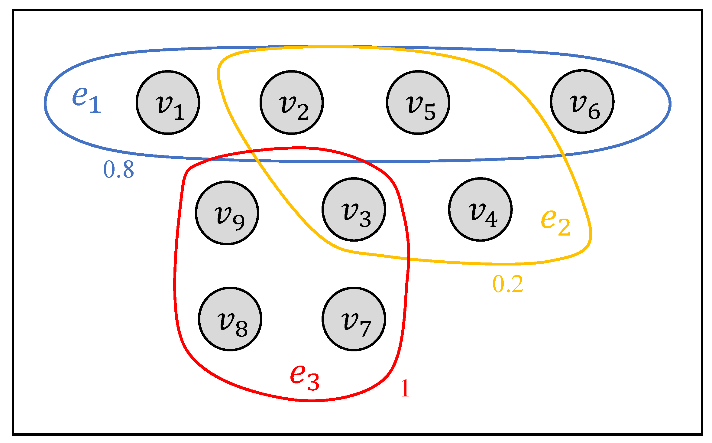
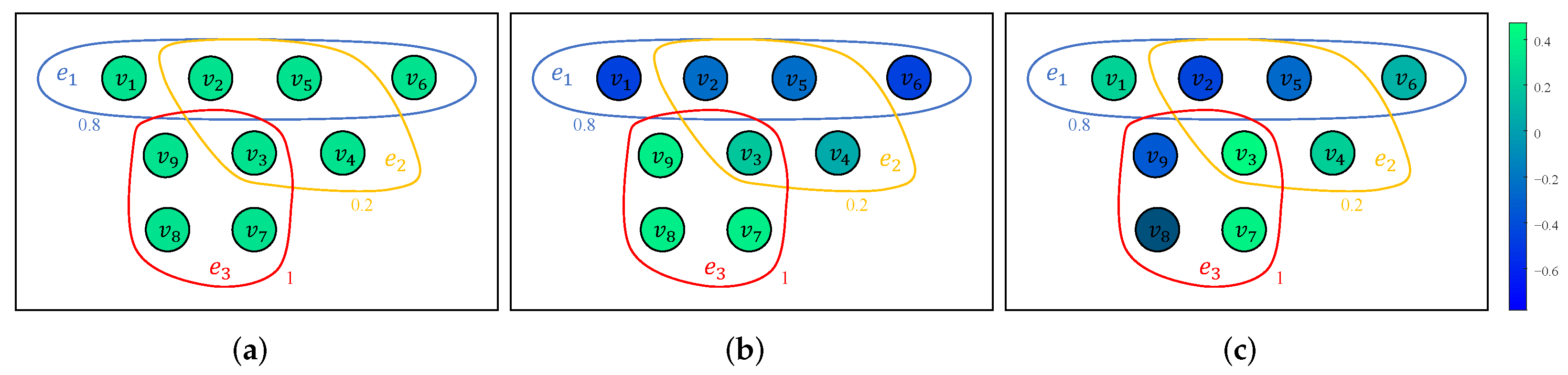
2. Hypergraph Signals

A weighted undirected hypergraph H = ( V , E , W ) consists of a vertex set V , a hyperedge set E and a diagonal hyperedge weight matrix W R 0 | E | × | E | . Each hyperedge e E E is a nonempty subset of the vertex set V . The cardinality of hyperedge e denotes the number of vertices e connects. If all hyperedges have the same cardinality c, the hypergraph is c-uniform. A real-valued HGS s : V R defined on the vertices of hypergraph H can be represented by a vector s R | V | , whose ith entry s i represents the signal value at the ith vertex in V .
Example 1.
The 4-uniform weighted undirected hypergraph in Figure 1 consists of nine vertices v i i = 1 9 and three 4-cardinality hyperedges { e i } i = 1 3 with weights equal to 0.8 , 0.2 and 1, respectively. The hyperedge e 1 connects four vertices, i.e., v 1 , v 2 , v 5 and v 6 .
In our work, we consider the weighted undirected hypergraph H = ( V , E , W ) as a c-uniform hypergraph with a signal s R | V | where c is an even number. If c is odd, we preprocess all hyperedges by adding an auxiliary vertex to each of them to make their cardinalities even in our previous work [36]. Specifically, we denote the preprocessed hypergraph by H = ( V , E , W ) where the weight matrix remains unchanged. Note that each auxiliary vertex only appears in one hyperedge. All | E | auxiliary vertices corresponding to each hyperedge are denoted by v i for i = | V | + 1 , , | V | + | E | , and the new vertex set V = V { v i } i = | V | + 1 | V | + | E | contains both original and auxiliary vertices. Each auxiliary vertex v | V | + i is added into the original hyperedge e i to obtain the new hyperedge e i represented by e i = e i { v | V | + i } . The signal at each auxiliary vertex v | V | + i in the new hyperedge e i is the arithmetic mean of signals on all vertices in the original hyperedge e i formulated as s aux = 1 c v i e s i . Thus, the preprocessed HGS s R | V | can be obtained by s = [ I | V | , 1 c H ] T s , in which matrices I | V | R | V | × | V | and H { 0 , 1 } | V | × | E | are the identity matrix and the incidence matrix of the original hypergraph H , respectively. We then can obtain a ( c + 1 ) -uniform hypergraph with even-cardinality hyperedges.
In the preprocessing, the introduction of the auxiliary vertices slightly changes the topology of the hypergraph. Specifically, it makes minor changes to the topology of each hyperedge locally, which still retains the global neighboring relationships of all | V | original vertices.
Example 2.
For simplicity, we consider a 3-cardinality hyperedge e = { v 1 , v 2 , v 3 } with weight w e = 1 in Figure 2. We preprocess it by adding an auxiliary vertex into e and obtain a new hyperedge e = e { v aux } . The weight of e remains 1, the vertex set becomes V { v aux } , and the signal at the auxiliary vertex is the arithmetic mean of signals on vertices { v i } i = 1 3 denoted by s aux = 1 3 i = 1 3 s i .
For a general hypergraph consisting of hyperedges with different cardinalities, we can preprocess all odd-cardinality hyperedges first. We then can divide the preprocessed hypergraph into a set of uniform partial hypergraphs with even cardinalities.

2.1. Total Variation of Hypergraph Signals

Inspired by the total variation of the graph signal, we generalize its notion to the total variation of the HGS to measure and describe the smoothness of the HGS over the hypergraph topology. Utilizing high-order adjacency tensors, the total variation of the HGS defined in [25] is not a homogeneous polynomial. Existing smoothness measures over hypergraphs [30] are combinations of pairwise smoothness measures in all hyperedges. Unlike those methods, we measure the smoothness of the HGS by a high-order homogeneous polynomial combining hyperedge-wise dissimilarities of signals.
We extend and define the HOTV of the HGS s over the c-uniform hypergraph H taking the form of
TV ( s ) 1 n ( c ) e E w e v i e ( s i s ¯ e ) c ,
where n ( c ) = ( c 1 ) c + c 1 c c normalizes the vertex degree for each hyperedge, w e denotes the weight of the hyperedge e , and s ¯ e 1 c v i e s i is the arithmetic mean of signals at each vertex in hyperedge e . s ¯ e can be viewed as the equally weighted linear aggregation of signals on all vertices in e . Each vertex in e is treated equivalently by the hyperedge and makes the same contribution to the HOTV over e . The HOTV considers the cth-order hyperedge-wise differences among signals rather than pairwise differences between signals. As a smoothness measure of the HGS s over the c-uniform hypergraph H where c is even, the HOTV is nonnegative for s R | V | . The HOTV equals zero if and only if vertices in each connected component of the hypergraph H take the same signal value. The HOTV will be small if the HGS obtains similar values on neighboring vertices, while the HOTV will be large if the HGS varies greatly over the topology.
When c = 2 , the hypergraph H becomes a graph and the total variation (1) has the same form as the quadratic form of graph Laplacians L formulated as
TV ( s ) = 2 e = { v i , v j } E w e ( ( s i s ¯ e ) 2 + ( s j s ¯ e ) 2 ) = e = { v i , v j } E w e ( s i s j ) 2 = s T L s .
Therefore, the total variation of graph signals can be considered as a special case of the proposed generalized HOTV.
Example 3.
The HOTV over the 4-uniform weighted hypergraph in Figure 1 is a quartic homogeneous polynomial given by
TV ( s ) = w e 1 v i e 1 ( s i s ¯ e 1 ) 4 + w e 2 v i e 2 ( s i s ¯ e 2 ) 4 + w e 3 v i e 3 ( s i s ¯ e 3 ) 4 = 0.8 v i { v 1 , v 2 , v 5 , v 6 } ( s i s 1 + s 2 + s 5 + s 6 4 ) 4 + 0.2 v i { v 2 , v 3 , v 4 , v 5 } ( s i s 2 + s 3 + s 4 + s 5 4 ) 4 + v i { v 3 , v 7 , v 8 , v 9 } ( s i s 3 + s 7 + s 8 + s 9 4 ) 4 ,
which can be seen as hyperedge-wise measuring the high-order dissimilarity among signals. When the HGS s obtains the same value at each vertex, each hyperedge-wise term in TV ( s ) and thus the whole TV ( s ) all equal zero.
For a preprocessed general hypergraph consisting of hyperedges with different even cardinalities, the HOTV (1) is no longer a homogeneous polynomial. Instead, it is the sum of the total variations of all the uniform partial hypergraphs formulated as
TV ( s ) = c C TV ( c ) ( s ) ,
where C is the cardinality set. The total variation of each uniform partial hypergraph is still a homogeneous polynomial. It is worth mentioning that the preprocessing of odd-cardinality partial hypergraphs ensures the nonnegative property of the total variation. Moreover, the hypergraph preprocessing does not change the intrinsic essence of the total variation, since the difference term corresponding to each auxiliary vertex equals zero and thus makes no contribution to the total variation. For clarity, we provide an example here to show how the minor changes of the topology slightly affect the difference polynomial and allow it to meet the definition of the total variation.
Example 4.
For simplicity, we continue considering the 3-cardinality hyperedge e = { v 1 , v 2 , v 3 } with weight 1 in Figure 2. The total variation over e is given by
TV ( s ) = 1 n ( 4 ) i = 1 3 ( s i s ¯ e ) 4 + ( s ¯ e s ¯ e ) 4 = 1 n ( 4 ) i = 1 3 ( s i s ¯ e ) 4 .
The difference term of the auxiliary vertex equals zero since s ¯ e = s ¯ e = 1 3 i = 1 3 s i . Obviously, the total variation over the new hyperedge e still only considers the difference between the signal at each original vertex and their arithmetic mean. The preprocessing of e changes only the order of the polynomial from 3 to 4, since TV ( s ) is defined only when c is even.

2.2. Tensor-Based Representations

As multidimensional arrays, tensors are a natural tool to mathematically represent hypergraph topologies and the corresponding high-order signals thanks to the flexibility of the tensor order. As a bijection between the index sets of two tensors that have the same size and different shapes, tensor reshaping such as tensor matricization and tensor vectorization can be utilized to equivalently represent any high-order HGS by various forms, such as matrix and vector forms. We will use operators mat ( · ) , vec ( · ) to represent the two kinds of tensor reshaping listed above and the operator ten ( · ) for the recovery from other forms to the tensor form.

2.2.1. Representations of Topologies

As mentioned in Section 2.1, the HOTV (1) measures the dissimilarity of the HGS. It can be rewritten as
TV ( s ) = 1 n ( c ) e E w e v i e ( c 1 c s i 1 c v j e { v i } s j ) c = 1 n ( c ) c c e E w e i = 1 c ( ( c e i 1 ) T Φ e s ) c = 1 n ( c ) c c e E w e i = 1 c ( Φ e T ( c e i 1 ) ) c × 1 s T × 2 × c s T = 1 n ( c ) c c e E w e i = 1 c ( Φ e T ( c e i 1 ) ) c s c ,
where the binary matrix Φ e R c × | V | samples all vertices in e from the vertex set V , the vector e i denotes the ith column of the c × c identity matrix I c , the vector 1 is a c-dimension all-ones vector, the operator ⊠ is the outer product of two vectors (or matrices), and the operator × n denotes the n-mode product of a tensor and a matrix. From (4), we can accordingly obtain a cth-order | V | -dimension hypergraph Laplacian tensor L ( c ) containing all information of the topology as an HGS difference operator formulated as
L ( c ) = 1 n ( c ) c c e E w e i = 1 c ( Φ e T ( c e i 1 ) ) c ,
which is found to coincide with the Laplacian tensor defined in [22]. The HOTV can then be represented by L ( c ) as
TV ( s ) = L ( c ) s c
for a c-uniform hypergraph, and
TV ( s ) = c C L ( c ) s c
for a general hypergraph. L ( c ) in (7) denotes the cth-order Laplacian tensor of the c-uniform partial hypergraph.
It is obvious from the definition (5) that the hypergraph Laplacian is supersymmetric [27], which means that its entries are invariant under any permutation of its indices. Moreover, according to both the nonnegative property of the HOTV and the hypergraph Laplacian form, we obtain Proposition 1 [22]. The definition of positive semidefinite tensors is presented below as well. In general, extended from the graph Laplacian, the even-order hypergraph Laplacian is a high-order difference operator which is supersymmetric and positive semidefinite as well.
Definition 1
(Positive semidefinite tensor). A real mth-order n-dimension supersymmetric tensor T = ( t i 1 , , i m ) , 1 i 1 , , i m n is positive semidefinite if for x R n , the homogeneous polynomial
T x m = T × 1 x T × 2 × m x T = i 1 , i m = 1 n t i 1 , , i m x i 1 x i m 0 .
Proposition 1.
Even-order hypergraph Laplacian tensors (5) are positive semidefinite.
For a preprocessed general hypergraph, we can obtain an even-order Laplacian tensor set according to the corresponding even-cardinality uniform partial hypergraph set. We can subsequently process the Laplacian tensor of each order accordingly.

2.2.2. Representations of Signals

For a real-valued HGS s R | V | , we introduce nonlinearity and define a high-order signal function s ( M ) : V × × V M R to obtain high-order signal values among vertices, where M = c / 2 and the operator × is the Cartesian product of two sets. The high-order HGS s ( M ) S ( M ) R | V | M is obtained by a nonlinear function of the original signal s formulated as
s ( M ) vec ( s M ) = s M ,
where S ( M ) is a subset of R | V | M formed by all values of s ( M ) for s R | V | , and the operator ⊗ denotes the Kronecker product of two vectors (or matrices). The supersymmetric rank-one [27,37] tensor s M = ten ( s ( M ) ) is the tensor form of the high-order HGS. We denote the set { 1 , , | V | } by [ | V | ] . For i 1 , i 2 , , i M [ | V | ] , the corresponding entry of s ( M ) is
( s ( M ) ) 1 + m = 1 M ( i m 1 ) | V | M m = s i 1 s i 2 s i M .
Remark (Sign ambiguity): There exists a problem introduced by the Mth-order signals when M = c / 2 is an even number. We cannot judge the sign of an HGS from the Mth-order form of the HGS. Instead, we can only determine the relative sign, namely, whether signals at any pair of vertices have the same or different signs. In this case, we may obtain the original HGS or a signal with the opposite sign from its high-order form. In semi-supervised or supervised learning tasks, we can determine the sign of an HGS by both the relative signs and signs of observations. For unsupervised learning tasks such as vertex clustering, it is enough to obtain distances or similarities of vertices from topologies that are irrelevant to signals. Therefore, although there may be no mapping from high-order signals to the original 1st-order ones due to the sign ambiguity, it does not matter in many practical applications. While degenerating into the graph case, namely, M = 1 , the high-order signal coincides with the original one and thus the above problem does not exist.

3. Hypergraph Fourier Transform

3.1. Construction of an Orthonormal Basis

We assume that the HGS is correlated to the topology and evolves smoothly over the topology since we construct the hypergraph based on high-order interactions among vertices. We need a basis for the HGS to capture the main features of the HGS and find relatively smooth representations of the HGS in a low-dimension vector space. Utilizing the high-order difference property of the HOTV (4), we can obtain the basis by decomposing the hypergraph Laplacian tensor. It is reasonable to treat each mode equivalently and obtain the same basis in the tensor decomposition since the tensor L ( c ) is supersymmetric. We require the basis vectors to be orthogonal since we hope for the HGS with distinct features to be irrelevant and to share no signal components. We then represent the orthonormal basis for R | V | , where the HGS is located, by a matrix U R | V | × | V | . Accordingly, the tensor decomposition formulated as
L ( c ) = G ( c ) × 1 U × 2 × c U
conforms to the Tucker decomposition form [27] which allows the core tensor G ( c ) not to be superdiagonal and assumes the basis U usually to be orthogonal. The decomposition (11) of L ( c ) with the basis U always exists owing to the existence and the non-uniqueness of the Tucker decomposition [27].
U M is an orthonormal matrix since we require U to be orthonormal. Considering high-order interactions among vertices, we can obtain the orthonormal basis U M for the high-order HGS by calculating the ith basis vector u i of U for i = 1 , , | V | in turn, which solves a functional minimization problem formulated as
u i M = arg min s ( M ) S ( M ) TV ( s ( M ) ) s . t . ( U i 1 M ) T s ( M ) = 0 s ( M ) T s ( M ) = 1 ,
where the operator ⊙ denotes the Khatri–Rao product of two matrices with the same number of columns and the matrix U i 1 M = [ u 1 M , , u i 1 M ] R | V | M × ( i 1 ) is only defined for i 2 . The first constraint in (12) containing i 1 equations denotes the orthogonal constraints of the basis vectors and only exists when i 2 . The second constraint in (12) requires the high-order signal to be normalized. By solving (12) iteratively, we can obtain a set of orthonormal high-order signals in a sequence that keeps the HOTV nondecreasing. In other words, for the ith problem, we obtain the smoothest signal as the basis vector which is orthogonal to the first i 1 obtained ones.
The constraint s ( M ) T s ( M ) = 1 is equivalent to s T s = 1 , since the real-valued signal satisfies s ( M ) T s ( M ) = ( s T s ) M = ( s T s ) M according to (9) and the inner product s T s is nonnegative. Thus, we can consider the 1st-order form of HGS s directly and rewrite (12) as
u i = arg min s R | V | TV ( s ) s . t . U i 1 T s = 0 s T s = 1 ,
where U i 1 = [ u 1 , , u i 1 ] R | V | × ( i 1 ) for i 2 . We provide a solution by the method of Lagrange multipliers and gradient descent method in Appendix A, since the problem (13) involves tensor operations such as tensor products and partial derivatives. As is also discussed in Appendix A, there may be nonzero off-diagonal entries in the core tensor G ( c ) for the Tucker decomposition, specifically with the basis U .
Example 5.
Three basis vectors u 1 , u 2 and u 8 of the example hypergraph H in Figure 1 are presented in Figure 3. As the first basis vector, namely the smoothest one, u 1 is a constant HGS over the topology with a zero total variation. The basis vector u 2 seems to provide an informative vertex clustering method corresponding to a specific smoothness of the HGS. Note that basis vectors associated with small total variations vary slowly over the topology, while basis vectors associated with larger total variations oscillate more rapidly and disorderly and tend to have more dissimilar values on vertices connected by large-weight hyperedges.
When c = 2 , problems (12) and (13) degenerate to the graph case and become exactly the same. By the Courant–Fischer theorem, the ith smallest eigenvalue λ i of a graph Laplacian matrix is the value of TV ( u i ) , and the corresponding eigenvector u i can be obtained by either (12) or (13). In either of the ways above, we can obtain a matrix U = [ u 1 , , u | V | ] which contains the basis of the graph Fourier transform (GFT) as its columns. Therefore, one can view the proposed orthonormal basis as a generalization of the GFT basis in the hypergraph case.

3.2. Hypergraph Fourier Transform

Given the orthonormal basis U generalized from the GFT basis, we define a novel HGFT by projecting signals to the orthonormal basis in order to process the high-order HGS in both vertex and spectral domains. The HGFT transforms the high-order vertex-domain HGS s ( M ) into the spectral-domain signal s ^ ( M ) , which can be formulated in both vector and tensor forms as
( vector form ) s ^ ( M ) ( U M ) T s ( M ) = ( U T s ) M
( tensor form ) ten ( s ^ ( M ) ) = ten ( s ( M ) ) × 1 U T × 2 × M U T = ( U T s ) M .
The inverse HGFT (IHGFT) is accordingly defined as
( vector form ) s ( M ) = U M s ^ ( M ) = ( U s ^ ) M
( tensor form ) ten ( s ( M ) ) = ten ( s ^ ( M ) ) × 1 U × 2 × M U = ( U s ^ ) M ,
which transforms a high-order spectral-domain signal s ^ ( M ) into its vertex-domain form s ( M ) . When M = 1 , all bases and signals in both the HGFT and the IHGFT are the same as those in the graph case.
Obviously, only orthogonal transformation is involved in either the HGFT or the IHGFT since U M is an orthonormal matrix. Therefore, signal transformations in both directions satisfy the conservation of energy.
To reduce the computational cost, we can calculate their equivalent forms (14) and (16) by the last step of each formula since (15) and (17) are all supersymmetric and rank-one. Moreover, both the HGFT (14) and the IHGFT (16) can degenerate into the transformation and its inverse of the original HGS given by
s ^ = U T s
and
s = U s ^
in some reducible cases of the follow-up work, since the sign ambiguity brought by high-order signals does not matter, as we have discussed in Section 2.2.

3.3. Spectral Form of Total Variation

After the construction of the orthomormal basis and the definition of the HGFT, the HOTV of the HGS in the spectral domain can be written as
TV ( s ) = L ( c ) × 1 s T × 2 × c s T = ( G ( c ) × 1 U × 2 × c U ) × 1 s T × 2 × c s T = G ( c ) × 1 ( s T U ) × 2 × c ( s T U ) = G ( c ) × 1 s ^ T × 2 × c s ^ T = G ( c ) s ^ c = TV ( s ^ )
according to (4) and (11). For 1 i | V | , the ith diagonal entry of G ( c ) denotes the HOTV of the ith basis vector of the HGS. Off-diagonal entries of G ( c ) correspond to invalid signal components since they do not belong to S ( M ) . As is mentioned above, since we introduce nonlinearity by defining and processing the high-order HGS, the subset S ( M ) is not a subspace of R | V | M . Therefore, those components are necessary for representing any valid HGS linearly even though they are invalid themselves.
In Section 3.2, we defined the spectral form of an HGS s as s ^ . We now analyze the spectral property of the HGS reflected by s ^ . The ith entry of s ^ is the coefficient of projecting s to the ith smoothest basis vector u i . Therefore, entries of s ^ reflect the spectral distribution of the HGS from low-frequency to high-frequency.
Example 6.
The total variation of an N × N image X under circular boundary conditions [38] can be viewed as the total variation of a 2-dimensional signal vec ( X ) R N 2 formulated as
TV ( X ) = vec ( X ) T L vec ( X ) ,
where L R N 2 × N 2 is the Laplacian matrix of the Cartesian product of two identical N-vertex unweighted loops. The Laplacian matrix L N of such N-vertex unweighted loop can always be diagonalized by the unitary discrete Fourier matrix V N C N × N formulated as L N = V N Λ V N T since it is circulant. Therefore, the Laplacian matrix
L = L N I N + I N L N
is circulant as well, and it can be diagonalized by the discrete Fourier matrix V = V N 2 [39,40]. The discrete Fourier transform (DFT) of the vectorized 2-dimensional signal vec ( x ) is implemented by vec ( X ^ ) = V T vec ( X ) .
Specifically, for a 2nd-order HGS s ( 2 ) , we can treat it as a special case of general 2-dimensional signals. If mat ( G ( 4 ) ) is a diagonal matrix, only all diagonal entries need to be considered as spectral coefficients. The total variation and the signal transformation we proposed are consistent with those of the above vectorized 2-dimensional signal vec ( X ) . The necessary and sufficient condition for mat ( G ( 4 ) ) to be diagonal is that G ( 4 ) is superdiagonal since G ( 4 ) is supersymmetric. The proof can be found in Appendix B. In other words, we assume that the hypergraph Laplacian L ( 4 ) can be orthogonally superdiagonalized by the basis U among all 4 modes in this special case.

4. Hypergraph Filters

In general, a hypergraph filter is a system which takes an HGS s as the input and obtains another HGS s ˜ as the output. The novel HGFT proposed in Section 3.2 provides both vertex and spectral perspectives for HGS filtering. We now consider a hypergraph filter F R | V | M × | V | M and denote its spectral form by F ^ R | V | M × | V | M . The filter in the two domains can be viewed as a function of L ( c ) and G ( c ) , respectively. In the vertex domain, we can filter a high-order HGS directly by
( vertex domain ) s ˜ ( M ) = F s ( M ) ,
while we filter a spectral-domain high-order signal by
( spectral domain ) s ^ ˜ ( M ) = F ^ s ^ ( M ) .
By substituting the HGFT and IHGFT into (24), any spectral filtering can be implemented in the vertex domain as
F = U M F ^ ( U M ) T .
For M = 1 , the hypergraph H degenerates into a graph, and (23) and (24) represent graph filtering in the vertex and spectral domains, respectively.
Filtering in either of the two domains takes linear transformations of high-order components as the results. However, the subset S ( M ) is defined to contain all vector forms of the Mth-order | V | -dimension supersymmetric rank-one tensors. Obviously, it is not a subspace and may not contain the column space of F . In this case, the subset S ( M ) does not satisfy the rules for vector addition and multiplication by real scalars. Thus, after implementing the linear combination of high-order components, the filtering result s ˜ ( M ) may not lie in the subset S ( M ) anymore. It may take an invalid form and not be able to reduce to the original 1st-order form as the filter output. In this case, we need to add the rank-one approximation (ROA) of ten ( s ˜ ( M ) ) into the filtering process to obtain a valid high-order signal form. The ROA of the supersymmetric tensor ten ( s ˜ ( M ) ) in the least-squares sense [41] solves a minimization problem formulated as
( λ ^ , u ^ ) = arg min λ R , u R | V | ten ( s ˜ ( M ) ) λ u M 2 2 s . t . u T u = 1
and arrives at the solution
ROA ( s ˜ ( M ) ) = λ ^ u ^ M ,
which preserves the most dominated supersymmetric rank-one component of ten ( s ˜ ( M ) ) in the least-squares sense. The relationship between the valid forms of (23) and (24) still maintains the correspondence of signals in both domains formulated as
ROA ( s ˜ ( M ) ) = U M ROA ( s ^ ˜ ( M ) )
where ROA ( · ) specifically denotes the equivalent vector operation of the tensor ROA, and the proof is given in Appendix C. In this way, we can ensure that taking the original HGS s as an input, the hypergraph filter can obtain a vector of the same size as its output. Outputs of a vertex-domain filter F and a spectral filter F ^ can be respectively obtained by
( vertex domain ) s ˜ = ( ROA ( s ˜ ( M ) ) ) 1 / M
and
( spectral domain ) s ^ ˜ = ( ROA ( s ^ ˜ ( M ) ) ) 1 / M ,
where ( · ) 1 / M denotes the inverse operation of the Kronecker products of M identical vectors. If M is odd, we can obtain the value of the ith entry by plugging i 1 = = i M = i into (10) and calculating its 1 / M th power. However, if M is even, we can only obtain the absolute value of the ith entry because of the sign ambiguity. The relative sign between signals at vertices v i and v j can be obtained by entries in (10) with { i m } m = 1 M composed of odd numbers of i and j. The final signs of signals can be determined according to signs of observations.
Example 7.
For the operator ( · ) 1 / M with an even M, according to (10), it can be learned from ( ROA ( s ˜ ( M ) ) ) 1 = s ˜ 1 M = 1 and ( ROA ( s ˜ ( M ) ) ) 1 + m = 1 M | V | M m = s ˜ 2 M = 1 that | s ˜ 1 | = | s ˜ 2 | = 1 1 / M = 1 . The signs of s ˜ 1 and s ˜ 2 are the same if ( ROA ( s ˜ ( M ) ) ) 1 + m = 2 M | V | M m = s ˜ 1 s ˜ 2 M 1 = 1 . The signs of s ˜ 1 and s ˜ 2 are different if ( ROA ( s ˜ ( M ) ) ) 1 + m = 2 M | V | M m = s ˜ 1 s ˜ 2 M 1 = 1 . We can judge the final sign of the HGS s ˜ according to signs of observations.
We now discuss two specific forms of hypergraph filters. One is polynomial filters which are based on the hypergraph Laplacians and can be operated in the vertex domain directly. The other one is reducible filters which can ensure that all high-order signals in the whole processing task are in valid forms and are able to degenerate into their 1st-order forms.

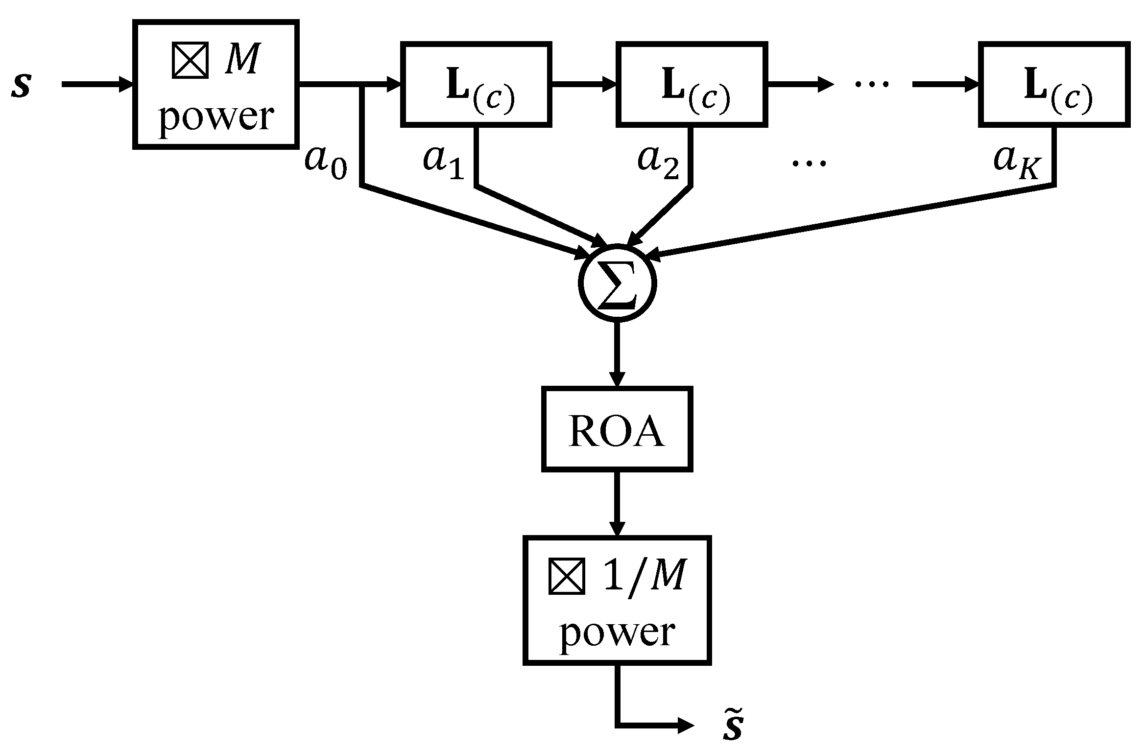
4.1. Polynomial Filters Based on the Hypergraph Laplacians

Polynomial hypergraph filters are a kind of common and handy filter which can be directly implemented in the vertex domain of the HGS. Taking vertex-domain signals as the input, we can construct a hypergraph polynomial filter based on the hypergraph Laplacians in Figure 4 formulated by
( vertex domain ) s ˜ = ( ROA ( k = 0 K a k mat ( L ( c ) ) k s ( M ) ) ) 1 / M = ( ROA ( k = 0 K a k s ˜ ( M ) ( k ) ) ) 1 / M ,
where K is the order of the polynomial filter, { a k } k = 0 K are the filter coefficients and s ˜ ( M ) ( k ) is the kth-order term of the hypergraph Laplacian filtering result. The whole filtering process can be divided into two parts. To obtain the kth-order term s ˜ ( M ) ( k ) , we process the high-order signal s ( M ) by L ( c ) for k times. Then, we take the linear combination of results of each order according to the filter coefficients, perform a rank-one approximation to obtain a valid high-order result and finally reduce it into its 1st-order form as the output of the filter. Regardless of whether the filtering result is valid or not, the computational cost of simply filtering an Mth-order | V | -vertex hypergraph signal is O ( ( K + 1 ) K 2 | V | 2 M ) , namely, O ( | V | c ) . The computational cost of the algorithm of the ROA of an Mth-order | V | -vertex hypergraph signal is O ( N iter i = 1 M | V | i ) , namely, O ( | V | M ) , where N iter denotes the number of iterations in the algorithm of the tensor ROA. Therefore, the computational cost of the high-order polynomial filter is O ( | V | c ) .
From the spectral perspective, by (28), we accordingly have
( spectral domain ) s ^ ˜ = ( ROA ( k = 0 K a k mat ( G ( c ) ) k s ^ ( M ) ) ) 1 / M .
As we have discussed before, the hypergraph Laplacian L ( c ) can be treated as a high-order difference operator, and G ( c ) takes high values on the positions corresponding to rapidly oscillating components in the tensor decomposition of L ( c ) . Therefore, L ( c ) can be regarded as a high-pass filter focusing on relatively greatly varying components of signals. We can utilize L ( c ) to process s ( M ) and mostly obtain the high-frequency components. Thus, the polynomial filter takes the ROA of the linear combination of the high-order HGS and its multi-order high-pass filtering results as the output.
When the filter coefficients { a k } k = 0 K take different values, we can obtain filters with distinct spectral properties for different applications. For instance, if smoothly varying components are more important and informative to the tasks, we can adjust the coefficients to remove the rapidly oscillating component from the input signal s ( M ) , namely, s ˜ ( M ) ( 0 ) , by utilizing the multi-order high-pass filtering results { s ˜ ( M ) ( k ) } k = 1 K in (31). The above operation can be considered as a low-pass filter.

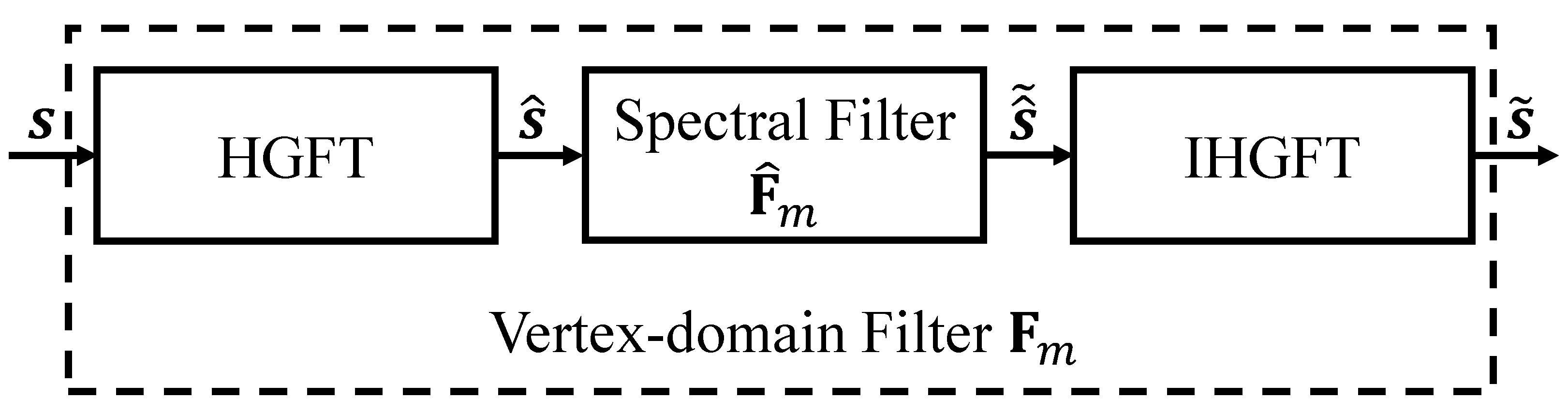
4.2. Reducible Filters
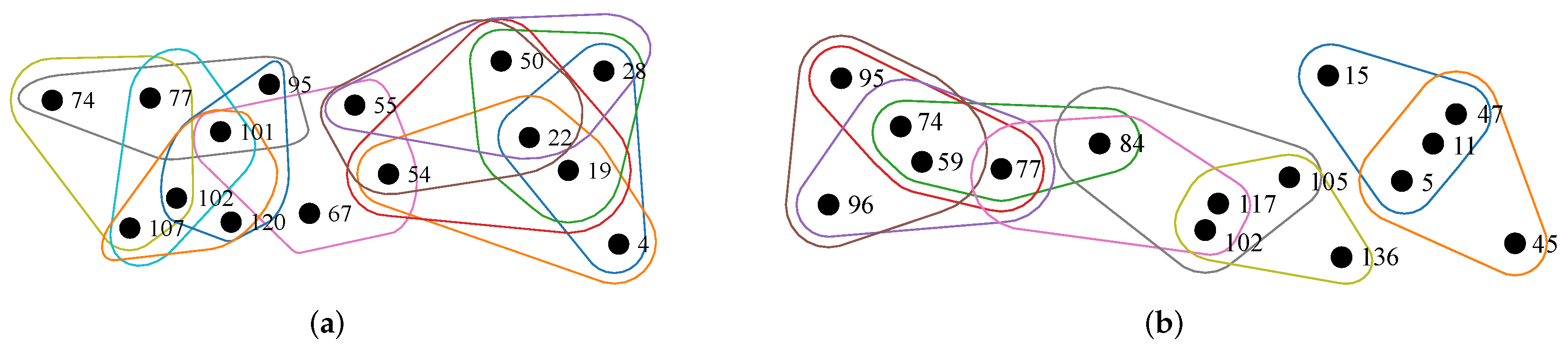
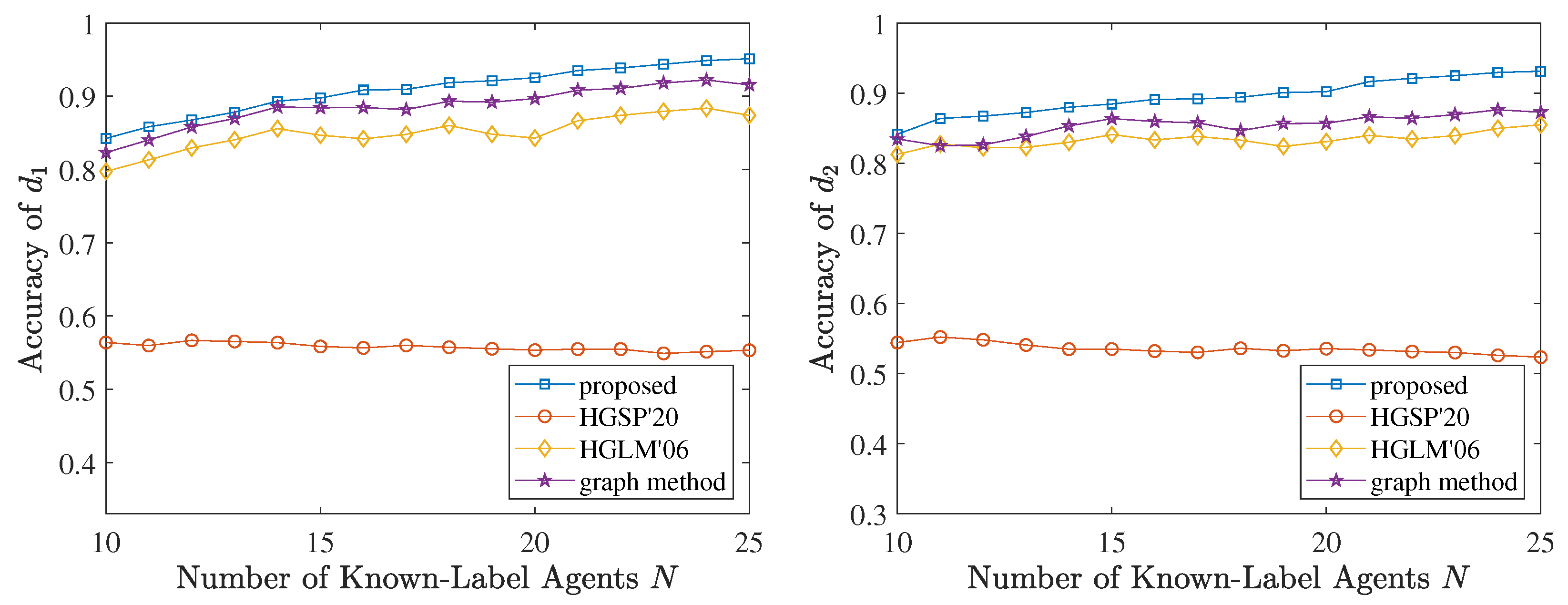
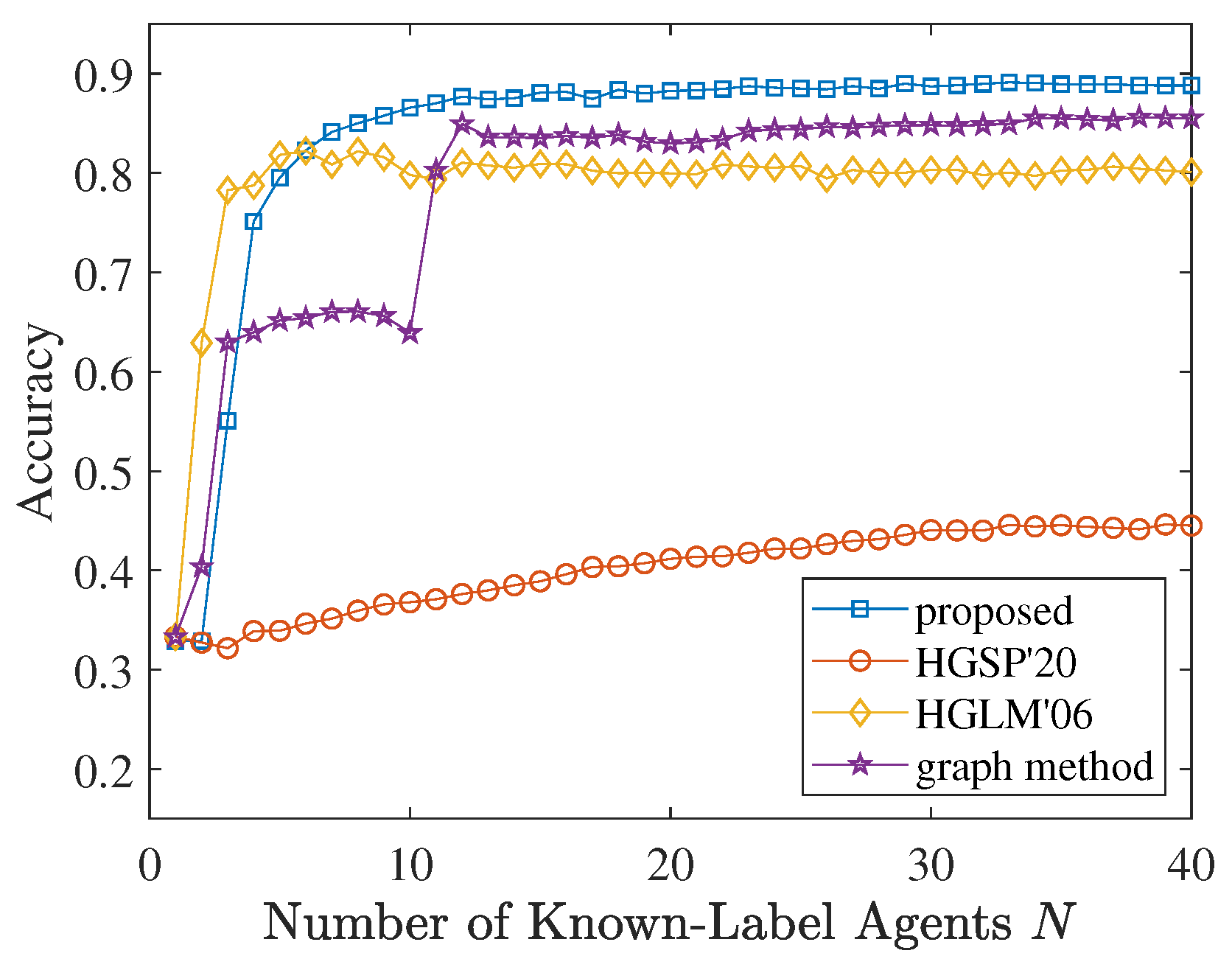
Reducible filters provide a way to ensure the validity of the high-order HGS throughout the whole filtering process. Thus, reducible filters do not need the ROA of the high-order HGS and allow the whole signal processing task to be equivalently implemented in a 1st-order way. More precisely, the reducibility requires filters in either of the two domains to be the Kronecker products of M identical matrices. We then can represent the spectral-domain filter by F ^ = F ^ m M , where F ^ m R | V | × | V | . By substituting the spectral form into (25), the corresponding vertex-domain form is F = ( U F ^ m U T ) M = F m M . Under this condition, hypergraph filtering in the vertex domain (23) and the spectral domain (24) can be precisely written as
( vertex domain ) s ˜ ( M ) = F m M s ( M ) = F m M s M = ( U F ^ m U T s ) M
and
( spectral domain ) s ^ ˜ ( M ) = F ^ m M s ^ ( M ) = ( F ^ m s ) M ,
and thus can be respectively reduced to
( vertex domain ) s ˜ = F m s = U F ^ m U T s
and
( spectral domain ) s ^ ˜ = F ^ m s ^
as Figure 5 shows.
As is mentioned in Section 2, the hypergraph H is undirected and does not take into account edge-dependent vertex weights [42], which means that all the c vertices in a hyperedge are treated equivalently. We hope that in each hyperedge, the way of signal transmission among the c vertices in the filtering process is the same for any direction to any vertex. Therefore, we constrain the tensor form of the filter F ^ to be supersymmetric. We then utilize the following proposition which is proven in Appendix D to filter the 1st-order HGS.
Proposition 2.
A real tensor ten ( F ^ ) = F ^ m M is supersymmetric for M 2 if and only if F ^ m is a real symmetric rank-one matrix or a zero matrix.
We now consider that a degenerate spectral filter F ^ m to be designed is a real symmetric rank-one matrix and takes the form F ^ m = λ m f ^ f ^ T where the unit vector f ^ R | V | and the scalar λ m R . The degenerate form of the vertex-domain reducible filtering (35) can then be rewritten as
s ˜ = λ m U f ^ f ^ T U T s = λ m ( U f ^ ) ( U f ^ ) T s .
It can be learned from (37) that f ^ i (the ith entry of f ^ ) corresponds to the ith component of the basis. By designing all the coefficients in f ^ , we obtain a unit vector U f ^ which is a signal with multiple spectral components. The filtering process is to project the signal s onto the unit vector U f ^ and then to multiply the projecting result by a coefficient λ m which includes the sign information and the amplitude gain of the filter. The smoothness property of the signal U f ^ directly determines the spectral components retained in the filtering process.
In general, as a function of G ( c ) , the original reducible filter F ^ = λ m M ( f ^ f ^ T ) M considers spectra corresponding to both valid and invalid high-order basis vectors and preserves a valid HGS form throughout the whole process simultaneously. Moreover, unlike some other filters, reducible filters can degenerate into a 1st-order form and thus provide outputs with intuitive spectral interpretations without the additional ROA.
While designing filters such as low-pass, high-pass, or band-pass filters, we can adjust the filter coefficients f ^ and λ m according to the practical demand. For example, the output of a low-pass filter tends to mainly concentrate on smooth HGS components represented by the first few basis vectors.

5. Application

As one of the widely studied supervised learning tasks, label learning studies a problem where each instance corresponds to a real-world agent associated with a label. The problem is to learn a function that predicts labels for unobserved instances according to some given observations. If features of all instances take the form of hypergraph topologies, the label learning task refers to hypergraph label learning specifically.
Hypergraph label learning has been widely applied to various scenarios such as automatic image annotation [43], visual classification of 2D or 3D objects [44,45,46], recommender systems [47,48], etc. Existing methods mostly utilize matrix-based or tensor-based forms to represent and process the HGS.

5.1. Hypergraph Label Learning Model

We model hypergraph labels by an HGS and implement hypergraph label learning in two steps. We first estimate the HGS by solving the following minimization problem
min s R | V | ( s , y , Ψ ) + λ Ω ( s ) ,
where the loss function measures the estimation error of known labels y , the regularization term Ω aims to avoid overfitting, the nonnegative parameter λ makes a trade-off between the above two terms, and Ψ is the sampling operator of the training set. We then set a threshold, divide all vertices into two categories according to the estimated signal and finally obtain the labels of the test set.
Concretely, we here provide a label learning method by directly filtering the 1st-order HGS, namely, using the degenerate form of reducible filters (37) by setting the filter coefficients λ m and f ^ appropriately. We assume that the HGS evolves smoothly over the topology and lies in a low-dimension vector space since we construct hypergraphs based on the vertex similarity and correlation. We then consider recovering signals by constraining it in a low-dimension linear subspace spanned by the first few vectors of the orthonormal basis. Therefore, given the number of vertices with known labels N, the last | V | N entries of f ^ are constrained to be zero, and the 1st-order HGS to be recovered can be represented by
s ˜ = λ m U f ^ f ^ T U T s = U Φ α ,
where Φ = [ I N , 0 N × ( | V | N ) ] T R | V | × N is a binary matrix and α = λ m Φ T f ^ f ^ T s ^ R N is the first N entries of the output of the 1st-order spectral reducible filter. For the sake of simplicity, instead of designing the coefficients λ m and f ^ of the reducible filter, we can filter the HGS by learning α whose dimension N is less than the number of the filter coefficients. However, a sufficiently large N possibly introduces the basis vector which is not smooth enough and tends to lead some large-variation components into the estimation of unknown labels. We thus consider to introduce a regularization term by constraining the values of α and sacrificing a little estimation accuracy since an appropriate N takes different values under different specific situations. In our experiment, we choose the square loss of known labels as the loss function and the squared 2 -norm of α as the regularization term Ω . The optimization problem (38) can then be rewritten as
min α R N Ψ U Φ α y 2 2 + λ α 2 2 .

5.2. Experimental Setups and Results

In this subsection, we provide two simulation examples over the acute inflammations dataset [49] and the iris dataset from the UCI Machine Learning Repository [50]. For the two datasets, we model them by 4-uniform weighted undirected hypergraphs based on the Euclidean distances of agents in their attribute vector space. The more similar the attribute vectors of any group G of 4 agents are, the more similar or correlated those agents seem to be and the more likely they are to be in one hyperedge. Therefore, in hypergraph topology constructions, we denote the arithmetic mean and the variance of the distance between any two agents in the group G by dist am = 1 4 2 { v i , v j } G dist ( v i , v j ) and dist var = 1 4 2 { v i , v j } G ( dist ( v i , v j ) dist am ) 2 , respectively. We then consider the values of dist am and dist var , and we accordingly set two thresholds τ am and τ var of the above two values to determine the existence of a hyperedge. We set τ am for two datasets equal to 0.5 and 0.07 , respectively, and set τ var for both datasets to select the 50 % smallest-variance hyperedges of all the hyperedges which have already met the threshold τ am . In addition, each vertex and its nearest group members must be in a hyperedge to ensure that no vertex is isolated. The weight of each hyperedge can be calculated by a Gaussian kernel function of dist am formulated as w = exp ( dist am 2 2 σ 2 ) where parameters σ of the two datasets are set to 2 2 and 1 / 2 respectively. Here, we provide 15-vertex sub-hypergraphs as examples for both datasets in Figure 6. The signal defined at each vertex is the classification label represented by a scalar (for a two-class dataset) or a three-dimensional vector (for a three-class dataset) taking the values from { 0 , 1 } , and the label classification threshold is set to 0.5 .
We compare the proposed factorization-based method with other three factorization-based methods. Given the same hypergraph topology, HGSP’20 [25] obtains its HGFT basis by the orthogonal CP decomposition [26] of the adjacency tensor in the HGSP framework. As one of the graph approximation methods [33], the method in [32] projects high-order interactions onto pairwise ones and defines a normalized hypergraph Laplacian matrix (HGLM) according to the same hypergraph topology. We can obtain an orthonormal basis by the eigendecomposition of the Laplacian matrix and we denote the method by HGLM’06. Focusing on pairwise interactions from the beginning, the graph method directly constructs a graph according to the same threshold τ am and the same weight function, ensures that no vertex is isolated, and uses the GFT basis for the task.
We first consider the disease diagnosis over the acute inflammations dataset with | V | = 120 potential patients and two diseases (as two labels) for each potential patient. The manifestation of the acute inflammation of the urinary bladder (denoted by label d 1 ) and acute nephritisis (denoted by label d 2 ) is provided as 6 attributes of each person such as temperature, the occurrence of nausea, etc. In each trial, we randomly choose 10–25 persons as agents with known labels and left the labels of the remaining persons unknown. We tested the learning accuracy for the two diseases (labels d 1 and d 2 ), respectively, by setting λ = 0 and taking the average of 1000-trial results, as shown in Figure 7.
In Figure 7, the proposed method performs best in the diagnosis accuracy of unknown-label potential patients, which indicates that the proposed orthonormal basis owns the most spectral information of both two signals in this situation. The spectral forms of the two signals are relatively sparse, and the signal components of the two signals tend to concentrate more on the low-frequency basis vectors. The performance of HGSP’20 is the least satisfactory here, likely because of the uncertainty caused by the orthogonal CP decomposition on some occasions. HGLM’06 does not perform as well as the proposed method probably due to the projection of high-order interactions onto pairwise ones. The projections and the subsequent mathematical representations bring irreversible information loss to the analysis of the HGS. The graph method also performs very well in the learning of the two labels. The reason why the graph method outperforms HGLM’06 is possibly that HGLM’06 focuses on the hypergraph topology at first and attaches a much larger weight to the edge onto which is projected by multiple large-weight hyperedges by the direct summation of the hyperedge weights. That might not be suitable in this case. In general, the two methods describe and utilize different pairwise interactions from different starting points.
In addition to the binary classification for each label, we also provide a three-class simulation example over the iris dataset with | V | = 150 agents. We model the three-class label of each agent by a three-dimensional binary vector, as mentioned before, and we solve the optimization problem (40) for each dimension by setting λ equal to 0, 0.007 and 0.007 , respectively. We test the label learning accuracy of unknown-label agents with the number of known labels N ranging from 1 to 40 by averaging 1000-repetition results. The comparative results are shown in Figure 8.
It can be observed in Figure 8 that the proposed method generally achieves a higher accuracy than other methods. For a very few N, HGLM’06 performs well and the accuracy increases rapidly, which indicates that its first few basis vectors do greatly help with the classification task. Both the proposed method and HGLM’06 behave well for a relatively small N, which shows the advantage of focusing on high-order interactions. Unlike those two methods, the graph method does not perform so well and it seems to need more labels to achieve a better result when N takes relatively small values. For a larger N, the graph method obtains more labels and performs a lot better. In summary, the above results show the advantage of the proposed method in this scenario and demonstrate the advantage of mining high-order interactions, especially under the lack of known labels.

6. Conclusions

To capture high-order interactions in complex structured signal processing, we propose an HGS analysis framework based on the hyperedge-wise HOTV proposed in this paper. The HOTV can be regarded as a smoothness measure of the HGS, and the hypergraph Laplacian obtained from the HOTV can be regarded as a high-order difference operator of the HGS. According to the smoothness measure, we construct an orthonormal basis reflecting spectral information of signals over the topology. We further propose a new signal transformation (a novel HGFT) and introduce both the vertex and the spectral domains of the HGS. We then implement hypergraph filtering in both domains equivalently and provide two specific filter forms. Finally, we validate the advantages of the proposed framework in some scenarios using applications in label learning and some experimental results.

Author Contributions

Conceptualization, R.Q. and H.F.; methodology, R.Q. and H.F.; software, R.Q.; validation, R.Q. and H.F.; formal analysis, R.Q.; investigation, R.Q.; resources, R.Q.; data curation, R.Q.; writing—original draft preparation, R.Q.; writing—review and editing, R.Q., H.F., C.X. and B.H.; visualization, R.Q.; supervision, H.F. and B.H.; project administration, H.F. and B.H.; funding acquisition, H.F. and B.H. All authors have read and agreed to the published version of the manuscript.

Funding

This work was supported by the Shanghai Municipal Natural Science Foundation (No. 19ZR1404700).

Institutional Review Board Statement

Not applicable.

Informed Consent Statement

Not applicable.

Data Availability Statement

Not applicable.

Conflicts of Interest

The authors declare no conflict of interest.

Abbreviations

The following abbreviations are used in this manuscript:
CPCANDECOMP/PARAFAC
GFTGraph Fourier transform
GSPGraph signal processing
HGFTHypergraph Fourier transform
HGLMHypergraph Laplacian matrix
HGSHypergraph signal
HGSPHypergraph signal processing
HOTVHigh-order total variation
IHGFTInverse hypergraph Fourier transform
ROARank-one approximation

Appendix A. Solution of Problem (13)

We provide a way to solve the problem here since the objective function of the problem (13) refers to tensor products. By the method of Lagrange multipliers, we can convert the minimization problem with i equality constraints into an unconstrained problem by first forming the Lagrangian function
L ( s , λ , μ ) = L ( c ) s c λ ( s T s 1 ) 𝟙 I s ( i ) j = 1 i 1 μ j u j T s ,
where I s = 2 , 3 , , | V | , 𝟙 I s ( i ) is an indicator function equal to 1 for i I s and 0 otherwise, and μ = [ μ 1 , , μ i 1 ] T R i 1 (for i = 1 , we only take the smoothness measure and the normalization constraint into consideration, and the last term of (A1) does not exist). The i constraint gradients u 1 , , u i 1 and 2 s of the ith minimization problem (13) are orthogonal and thus linearly independent. Therefore, the first-order necessary condition (Lagrange multipliers) holds by Proposition 3.1.1 in [51]. We set the gradient of (A1) to zero and arrive at
s , λ , μ L ( s , λ , μ ) = [ s L T , λ L , μ L T ] T = 0 ,
the solutions of which are all candidates of the optimal solution including the global optimal one since the optimal problem is nonconvex. Specifically, the partial derivative of the Lagrangian function with respect to s in (A2) is formulated as
s L = c L ( c ) s c 1 2 λ s 𝟙 I s ( i ) j = 1 i 1 μ j u j .
It is worth noting that (A3) involves partial derivatives of tensor products [52] which are formulated as
s ( L ( c ) s c ) = c L ( c ) × 2 s T × 3 × c s T = c L ( c ) s c 1 .
According to (A2) and (A3), by s T ( s L ) = 0 and U i 1 T ( s L ) = 0 , the multipliers λ and μ can be solved and represented by s as
λ = c 2 L ( c ) s c ,
and
μ j = c u j T L ( c ) s c 1 , j [ i 1 ] .
By plugging (A5) and (A6) into (A3), we have
s L = ( I | V | s s T U i 1 U i 1 T ) c L ( c ) s c 1 .
We can arrive at a solution corresponding to a local minimum of the objective function using the gradient descent method by iterating
s k + 1 = s k η ( s L ) | s = s k = s k η ( I | V | s k s k T i 1 U i 1 T ) c L ( c ) s k c 1
where the stepsize η > 0 .
Using the solutions U of the | V | problems as the basis, the tensor decomposition (11) takes the form of the Tucker decomposition [27]. We can view the first basis vector in U from the perspective of Z-eigenpairs of supersymmetric tensors [52]. According to (A2) and (A7), solutions corresponding to any local minimum of the objective function all satisfy
( I | V | s s T U i 1 U i 1 T ) c L ( c ) s c 1 = 0
which indicates that the vector L ( c ) s c 1 belongs to the nullspace of ( I | V | s s T U i 1 U i 1 T ) , namely, the column space of [ U i 1 , s ] . Specifically, following from (A5), when i = 1 , (A9) can be written as L ( c ) u 1 c 1 = 0 u 1 which takes the form of Z-eigenpairs of L ( c ) . The Z-eigenvector u 1 can be 1 | V | 1 which is the smoothest signal over any topology with the corresponding Z-eigenvalue 0 as the smallest one. However, when i 2 , L ( c ) u 1 c 1 may no longer be consistent with the form of Z-eigenpairs, which indicates that there may be nonzero off-diagonal elements in the core tensor G ( c ) in (11). Therefore, we represent the Laplacian tensor L ( c ) in the form of the Tucker decomposition by the orthonormal basis.
For general hypergraphs, we can find the local minimum of TV ( s ) and the corresponding ith basis vector in a similar way. In this case, the Lagrange multipliers (A5) and (A6) respectively become
λ = 1 2 c C c L ( c ) s c
and
μ j = u j T c C c L ( c ) s c 1 , for j [ i 1 ] .
The partial derivative of the Lagrangian function (A3) with respect to s accordingly changes to
s L = ( I | V | s s T U i 1 U i 1 T ) c C c L ( c ) s c 1 .
We can also obtain a local minimum of the problem using the gradient descent method by iterating
s k + 1 = s k η ( s L ) | s = s k = s k η ( I | V | s k s k T U i 1 U i 1 T ) c C c L ( c ) s k c 1 ,
where the step size η > 0 .

Appendix B

Proposition A1.
mat ( G ( 4 ) ) is a diagonal matrix if and only if the supersymmetric tensor G ( 4 ) is superdiagonal.
Proof. 
For an even number c > 0 , the two forms, G ( c ) and mat ( G ( c ) ) , are equivalent representations with entries
( G ( c ) ) i 1 , , i c = ( mat ( G ( c ) ) ) 1 + m = 1 M ( i m 1 ) | V | M m , 1 + m = M + 1 c ( i m 1 ) | V | c m for i 1 , , i c [ | V | ]
since either of them can be obtained from the other by tensor reshaping. We define functions g 1 : [ | V | ] × × [ | V | ] M   [ | V | M ] and g 2 : [ | V | ] × × [ | V | ] M   [ [ | V | M ] to describe the way indices of G ( c ) map to indices of mat ( G ( c ) ) , by which (A14) can be simplified as
( G ( c ) ) i 1 , , i c = ( mat ( G ( c ) ) ) g 1 ( i 1 , , i M ) , g 2 ( i M + 1 , , i c ) for i 1 , , i c [ | V | ] .
Entries of mat ( G ( c ) ) with indices satisfying
i m = i m + M [ | V | ] for m { 1 , , M }
are the | V | M diagonal entries of mat ( G ( c ) ) . Entries of G ( c ) with indices i 1 = = i c [ | V | ] are the | V | superdiagonal entries of G ( c ) .
For the sufficiency, mat ( G ( c ) ) is a diagonal matrix if G ( c ) is a superdiagonal tensor, since all the | V | superdiagonal entries of G ( c ) correspond to the | V | diagonal entries of mat ( G ( c ) ) .
For the purpose of this study, we already know that mat ( G ( c ) ) is a diagonal matrix. We then consider the | V | M | V | diagonal entries of mat ( G ( c ) ) that correspond to entries off the superdiagonal line of G ( c ) . G ( c ) is a superdiagonal tensor if all those entries are zero. Indices of those entries take at least two distinct values from [ | V | ] . Therefore, all those entries can be denoted by ( mat ( G ( c ) ) ) g 1 ( i 1 , , i m 1 , , i m 2 , , i M ) , g 2 ( i M + 1 , , i m 1 + M , , i m 2 + M , , i c ) where i m 1 = i m 1 + M i m 2 = i m 2 + M and 1 m 1 < m 2 M . The supersymmetry of G ( c ) requires
( mat ( G ( c ) ) ) g 1 ( i 1 , , i m 1 , , i m 2 , , i M ) , g 2 ( i M + 1 , , i m 1 + M , , i m 2 + M , , i c ) = ( mat ( G ( c ) ) ) g 1 ( i 1 , , i m 2 , , i m 1 , , i M ) , g 2 ( i M + 1 , , i m 1 + M , , i m 2 + M , , i c ) .
The last equality in (A17) is an off-diagonal entry of the diagonal matrix since its index does not satisfy (A16). Therefore, (A17) equals zero. That is, all those diagonal entries of mat ( G ( c ) ) that correspond to entries off the superdiagonal line of G ( c ) are zero. We then complete the proof that G ( c ) is superdiagonal.
Therefore, specifically for c = 4 , the proof of Proposition A1 is completed. □

Appendix C. Proof of (28)

( λ ^ , u ^ ) = arg min λ R , u R | V | ( s ˜ ( M ) , λ , u ) s . t . u T u = 1 ,
We use ( s ˜ ( M ) , λ , u ) to denote the objective function in (26) which can be rewritten as
( s ˜ ( M ) , λ , u ) = ten ( U M s ^ ˜ ( M ) λ u M ) 2 2 = U M ( s ^ ˜ ( M ) λ ( U M ) T u M ) 2 2 = U M ( s ^ ˜ ( M ) λ ( U T u ) M ) 2 2 = s ^ ˜ ( M ) λ ( U T u ) M 2 2 = ten ( s ^ ˜ ( M ) ) λ ( U T u ) M 2 2 = ( s ^ ˜ ( M ) , λ , U T u )
by utilizing the IHGFT (16) and the orthonormal property of the matrix U M . It can be learned from (A18) that the problem (26) can solve the ROA of both ten ( s ˜ ( M ) ) and ten ( s ^ ˜ ( M ) ) . Similar to (27), the final solution of ten ( s ^ ˜ ( M ) ) is accordingly given by
ROA ( s ^ ˜ ( M ) ) = λ ^ ( U T u ^ ) M .
Therefore, we have (28) according to (27) and (A19).

Appendix D. Proof of Proposition 2

Consider the tensor ten ( F ^ ) = F ^ m M for M 2 and its entry
( ten ( F ^ ) ) i 1 , , i c = m = 1 M ( F ^ m ) i 2 m 1 , i 2 m for i 1 , , i c [ | V | ] .
For the sake of sufficiency, both the real symmetric rank-one matrix and the zero matrix allow F ^ m to take the form of F ^ m = λ m f ^ f ^ T = λ m f ^ f ^ where the unit vector f ^ R | V | and the scalar λ m R . Then, ten ( F ^ ) takes the form
ten ( F ^ ) = ( λ m f ^ f ^ ) M = λ m M f ^ c ,
and consequently is supersymmetric.
For the purposes of this work, ten ( F ^ ) is supersymmetric, and thus there should be no change under any permutation of the tensor indices. Since ten ( F ^ ) is defined by F ^ m , we first think about the intrapair exchange which exchanges two indices of the matrix F ^ m . Any intrapair exchange will keep ten ( F ^ ) unchanged, and therefore we have
ten ( F ^ ) = F ^ m T F ^ m M 1
which indicates that F ^ m should be symmetric. In addition to intra-pair exchanges, we also need to take into account interpair exchanges, namely, exchanges of indices in two different matrices. We might exchange the 1st and the 3rd indices of ten ( F ^ ) , and we will arrive at
( ten ( F ^ ) ) i 1 , , i c = ( F ^ m ) i 3 , i 2 ( F ^ m ) i 1 , i 4 m = 3 M ( F ^ m ) i 2 m 1 , i 2 m for i 1 , , i c [ | V | ] .
If the supersymmetric tensor ten ( F ^ ) is not a zero tensor, F ^ m is not a zero matrix. We then can learn from (A20) and (A23) that
( F ^ m ) i 1 , i 2 ( F ^ m ) i 3 , i 4 = ( F ^ m ) i 3 , i 2 ( F ^ m ) i 1 , i 4 for i 1 , , i 4 [ | V | ] .
We now denote the ith column of F ^ m by col F ^ m ( i ) , and then (A24) can be rewritten as
col F ^ m ( i 2 ) col F ^ m ( i 4 ) T = col F ^ m ( i 4 ) col F ^ m ( i 2 ) T for i 2 , i 4 [ | V | ] .
It is obvious that (A25) shows the symmetry of the matrix col F ^ m ( i 2 ) col F ^ m ( i 4 ) T for the two indices i 2 , i 4 with arbitrary values. Therefore, each column of F ^ m is parallel to the others, which implies that F ^ m is rank-one.
If the supersymmetric tensor ten ( F ^ ) is a zero tensor, F ^ m is a zero matrix.
Therefore, F ^ m is a real symmetric rank-one matrix or a zero matrix if ten ( F ^ ) is real and supersymmetric.
Thus, we have completed the proof of the necessary and sufficient condition for the real tensor ten ( F ^ ) = F ^ m M to be supersymmetric.

References

  1. Shuman, D.I.; Narang, S.K.; Frossard, P.; Ortega, A.; Vandergheynst, P. The emerging field of signal processing on graphs: Extending high-dimensional data analysis to networks and other irregular domains. IEEE Signal Process. Mag. 2013, 30, 83–98. [Google Scholar] [CrossRef] [Green Version]
  2. Sandryhaila, A.; Moura, J.M. Discrete signal processing on graphs: Frequency analysis. IEEE Trans. Signal Process. 2014, 62, 3042–3054. [Google Scholar] [CrossRef] [Green Version]
  3. Ortega, A.; Frossard, P.; Kovacevic, J.; Moura, J.M.; Vandergheynst, P. Graph Signal Processing: Overview, Challenges, and Applications. Proc. IEEE 2018, 106, 808–828. [Google Scholar] [CrossRef] [Green Version]
  4. Benson, A.R.; Gleich, D.F.; Leskovec, J. Higher-order organization of complex networks. Science 2016, 353, 163–166. [Google Scholar] [CrossRef] [Green Version]
  5. Gu, X.; Chen, L.; Krenn, M. Quantum experiments and hypergraphs: Multiphoton sources for quantum interference, quantum computation, and quantum entanglement. Phys. Rev. A 2020, 101, 33816. [Google Scholar] [CrossRef] [Green Version]
  6. Duck, I. Three-alpha-particle resonances via the Fadeev equation. Nucl. Phys. 1966, 84, 586–594. [Google Scholar] [CrossRef]
  7. Kim, H.Y.; Sofo, J.O.; Velegol, D.; Cole, M.W.; Lucas, A.A. Van der Waals forces between nanoclusters: Importance of many-body effects. J. Chem. Phys. 2006, 124, 74504. [Google Scholar] [CrossRef]
  8. Petri, G.; Expert, P.; Turkheimer, F.; Carhart-Harris, R.; Nutt, D.; Hellyer, P.J.; Vaccarino, F. Homological scaffolds of brain functional networks. J. R. Soc. Interface 2014, 11, 20140873. [Google Scholar] [CrossRef] [Green Version]
  9. Sizemore, A.E.; Giusti, C.; Kahn, A.; Vettel, J.M.; Betzel, R.F.; Bassett, D.S. Cliques and cavities in the human connectome. J. Comput. Neurosci. 2018, 44, 115–145. [Google Scholar] [CrossRef] [Green Version]
  10. Abrams, P.A. Arguments in Favor of Higher Order Interactions. Am. Nat. 1983, 121, 887–891. [Google Scholar] [CrossRef]
  11. Mayfield, M.M.; Stouffer, D.B. Higher-order interactions capture unexplained complexity in diverse communities. Nat. Ecol. Evol. 2017, 1, 0062. [Google Scholar] [CrossRef] [PubMed]
  12. Grilli, J.; Barabás, G.; Michalska-Smith, M.J.; Allesina, S. Higher-order interactions stabilize dynamics in competitive network models. Nature 2017, 548, 210–213. [Google Scholar] [CrossRef] [PubMed]
  13. Cervantes-Loreto, A.; Ayers, C.A.; Dobbs, E.K.; Brosi, B.J.; Stouffer, D.B. The context dependency of pollinator interference: How environmental conditions and co-foraging species impact floral visitation. Ecol. Lett. 2021, 24, 1443–1454. [Google Scholar] [CrossRef] [PubMed]
  14. Ritz, A.; Tegge, A.N.; Kim, H.; Poirel, C.L.; Murali, T.M. Signaling hypergraphs. Trends Biotechnol. 2014, 32, 356–362. [Google Scholar] [CrossRef] [PubMed] [Green Version]
  15. Sanchez-Gorostiaga, A.; Bajić, D.; Osborne, M.L.; Poyatos, J.F.; Sanchez, A. High-order interactions dominate the functional landscape of microbial consortia. bioRxiv 2018, 333534. [Google Scholar] [CrossRef] [Green Version]
  16. Battiston, F.; Cencetti, G.; Iacopini, I.; Latora, V.; Lucas, M.; Patania, A.; Young, J.G.; Petri, G. Networks beyond pairwise interactions: Structure and dynamics. Phys. Rep. 2020, 874, 1–92. [Google Scholar] [CrossRef]
  17. Battiston, F.; Amico, E.; Barrat, A.; Bianconi, G.; Ferraz de Arruda, G.; Franceschiello, B.; Iacopini, I.; Kéfi, S.; Latora, V.; Moreno, Y.; et al. The physics of higher-order interactions in complex systems. Nat. Phys. 2021, 17, 1093–1098. [Google Scholar] [CrossRef]
  18. Berge, C. Graphs and Hypergraphs; North-Holland Pub. Co.: Amsterdam, The Netherlands, 1973. [Google Scholar]
  19. Cooper, J.; Dutle, A. Spectra of uniform hypergraphs. Linear Algebra Appl. 2012, 436, 3268–3292. [Google Scholar] [CrossRef] [Green Version]
  20. Qi, L. H+-eigenvalues of Laplacian tensor and signless Laplacians. Commun. Math. Sci. 2014, 12, 1045–1064. [Google Scholar] [CrossRef] [Green Version]
  21. Banerjee, A.; Char, A.; Mondal, B. Spectra of general hypergraphs. Linear Algebra Appl. 2017, 518, 14–30. [Google Scholar] [CrossRef] [Green Version]
  22. Hu, S.; Qi, L. Algebraic connectivity of an even uniform hypergraph. J. Comb. Optim. 2012, 24, 564–579. [Google Scholar] [CrossRef]
  23. Chang, J.; Chen, Y.; Qi, L.; Yan, H. Hypergraph clustering using a new laplacian tensor with applications in image processing. SIAM J. Imag. Sci. 2020, 13, 1157–1178. [Google Scholar] [CrossRef]
  24. Ouvrard, X.; Le Goff, J.M.; Marchand-Maillet, S. On Adjacency and e-Adjacency in General Hypergraphs: Towards a New e-Adjacency Tensor. Electron. Notes Discret. Math. 2018, 70, 71–76. [Google Scholar] [CrossRef] [Green Version]
  25. Zhang, S.; Ding, Z.; Cui, S. Introducing Hypergraph Signal Processing: Theoretical Foundation and Practical Applications. IEEE Internet Things 2020, 7, 639–660. [Google Scholar] [CrossRef] [Green Version]
  26. Afshar, A.; Perros, I.; Ho, J.C.; Khalil, E.B.; Sunderam, V.; Dilkina, B.; Xiong, L. CP-ORTHO: An Orthogonal Tensor Factorization Framework for Spatio-Temporal Data. In Proceedings of the GIS Proc. ACM International Symposium on Advances in Geographic Information Systems, SIGSPATIAL’17, Redondo Beach, CA, USA, 7–10 November 2017; Association for Computing Machinery: New York, NY, USA, 2017; Volume 2017-Novem. [Google Scholar] [CrossRef]
  27. Kolda, T.G.; Bader, B.W. Tensor decompositions and applications. SIAM Rev. 2009, 51, 455–500. [Google Scholar] [CrossRef]
  28. Comon, P.; Golub, G.; Lim, L.H.; Mourrain, B. Symmetric Tensors and Symmetric Tensor Rank. SIAM J. Matrix Anal. Appl. 2008, 30, 1254–1279. [Google Scholar] [CrossRef] [Green Version]
  29. Hein, M.; Setzer, S.; Jost, L.; Rangapuram, S.S. The total variation on hypergraphs-learning on hypergraphs revisited. Adv. Neural Inf. Process. Syst. 2013, 26. Available online: https://proceedings.neurips.cc/paper/2013/hash/8a3363abe792db2d8761d6403605aeb7-Abstract.html (accessed on 14 January 2022).
  30. Nguyen, C.H.; Mamitsuka, H. Learning on Hypergraphs With Sparsity. IEEE Trans. Pattern Anal. Mach. Intell. 2021, 43, 2710–2722. [Google Scholar] [CrossRef] [Green Version]
  31. Zien, J.Y.; Schlag, M.D.; Chan, P.K. Multilevel spectral hypergraph partitioning with arbitrary vertex sizes. IEEE Trans. Comput. Des. Integr. Circuits Syst. 1999, 18, 1389–1399. [Google Scholar] [CrossRef]
  32. Zhou, D.; Huang, J.; Schölkopf, B. Learning with Hypergraphs: Clustering, Classification, and Embedding. In Proceedings of the 19th International Conference on Neural Information Processing Systems, Vancouver, BC, Canada, 4–7 December 2006; MIT Press: Cambridge, MA, USA, 2006; pp. 1601–1608. [Google Scholar]
  33. Agarwal, S.; Branson, K.; Belongie, S. Higher order learning with graphs. In Proceedings of the 23rd International Conference on Machine Learning ( ICML ’06), Pittsburgh, PA, USA, 25–29 June 2006; Association for Computing Machinery: New York, NY, USA, 2006; Volume 148, pp. 17–24. [Google Scholar] [CrossRef] [Green Version]
  34. Barbarossa, S.; Tsitsvero, M. An introduction to hypergraph signal processing. In Proceedings of the 2016 IEEE International Conference on Acoustics, Speech and Signal Processing (ICASSP), Shanghai, China, 20–25 March 2016; Volume 2016-May, pp. 6425–6429. [Google Scholar] [CrossRef]
  35. Barbarossa, S.; Sardellitti, S. Topological Signal Processing over Simplicial Complexes. IEEE Trans. Signal Process. 2020, 68, 2992–3007. [Google Scholar] [CrossRef] [Green Version]
  36. Qu, R.; He, J.; Feng, H.; Xu, C.; Hu, B. Regularized recovery by multi-order partial hypergraph total variation. In Proceedings of the ICASSP—2021 IEEE International Conference on Acoustics, Speech and Signal Processing (ICASSP), Virtual, 6–12 June 2021; Volume 2021-June, pp. 2930–2934. [Google Scholar] [CrossRef]
  37. Bourbaki, N. Elements of Mathematics, Algebra I, Chapter 1–3; Springer: Berlin/Heidelberg, Germany, 1989; ISBN 3-540-64243-9. [Google Scholar]
  38. Ng, M.K.; Weiss, P.; Yuan, X. Solving constrained total-variation image restoration and reconstruction problems via alternating direction methods. SIAM J. Sci. Comput. 2010, 32, 2710–2736. [Google Scholar] [CrossRef]
  39. Fiedler, M. Algebraic connectivity of graphs. Czechoslov. Math. J. 1973, 23, 298–305. [Google Scholar] [CrossRef]
  40. Barik, S.; Bapat, R.B.; Pati, S. On the laplacian spectra of product graphs. Appl. Anal. Discret. Math. 2015, 9, 39–58. [Google Scholar] [CrossRef] [Green Version]
  41. Kofidis, E.; Regalia, P.A. On the best rank-1 approximation of higher-order supersymmetric tensors. SIAM J. Matrix Anal. Appl. 2002, 23, 863–884. [Google Scholar] [CrossRef] [Green Version]
  42. Chitra, U.; Raphael, B.J. Random walks on hypergraphs with edge-dependent vertex weights. In Proceedings of the 36th International Conference on Machine Learning (ICML 2019), Long Beach, CA, USA, 9–15 June 2019; Proceedings of Machine Learning Research. Chaudhuri, K., Salakhutdinov, R., Eds.; 2019; Volume 97, pp. 2002–2011. [Google Scholar]
  43. Tang, C.; Liu, X.; Wang, P.; Zhang, C.; Li, M.; Wang, L. Adaptive Hypergraph Embedded Semi-Supervised Multi-Label Image Annotation. IEEE Trans. Multimed. 2019, 21, 2837–2849. [Google Scholar] [CrossRef]
  44. Yu, J.; Tao, D.; Wang, M. Adaptive hypergraph learning and its application in image classification. IEEE Trans. Image Process. 2012, 21, 3262–3272. [Google Scholar] [CrossRef] [PubMed]
  45. Wang, M.; Liu, X.; Wu, X. Visual Classification by ℓ1-Hypergraph Modeling. IEEE Trans. Knowl. Data Eng. 2015, 27, 2564–2574. [Google Scholar] [CrossRef]
  46. Zhang, Z.; Lin, H.; Zhao, X.; Ji, R.; Gao, Y. Inductive Multi-Hypergraph Learning and Its Application on View-Based 3D Object Classification. IEEE Trans. Image Process. 2018, 27, 5957–5968. [Google Scholar] [CrossRef]
  47. Van Lierde, H.; Chow, T.W.S. A Hypergraph Model for Incorporating Social Interactions in Collaborative Filtering. In Proceedings of the 2017 International Conference on Data Mining, Communications and Information Technology (DMCIT 2017), Phuket, Thailand, 25–27 May 2017; Association for Computing Machinery: New York, NY, USA, 2017. [Google Scholar] [CrossRef]
  48. Gharahighehi, A.; Vens, C.; Pliakos, K. An Ensemble Hypergraph Learning Framework for Recommendation. In Discovery Science, Proceedings of the 24th International Conference, DS 2021; Halifax, NS, Canada, 11–13 October 2021; Carlos, S., Torgo, L., Eds.; Springer International Publishing: Cham, Switzerland, 2021; pp. 295–304. [Google Scholar] [CrossRef]
  49. Czerniak, J.; Zarzycki, H. Application of rough sets in the presumptive diagnosis of urinary system diseases. In Artificial Intelligence and Security in Computing Systems; Springer: Boston, MA, USA, 2003; pp. 41–51. [Google Scholar] [CrossRef]
  50. Dua, D.; Graff, C. UCI Machine Learning Repository; University of California, Irvine, School of Information and Computer Sciences: Irvine, CA, USA, 2019. [Google Scholar]
  51. Bertsekas, D.P. Nonlinear Programming; Athena Scientific: Belmont, MA, USA, 1999. [Google Scholar]
  52. Qi, L. Eigenvalues of a real supersymmetric tensor. J. Symb. Comput. 2005, 40, 1302–1324. [Google Scholar] [CrossRef] [Green Version]
Figure 1. An example of 4-uniform weighted undirected hypergraphs.
Symmetry 14 00543 g001
Figure 2. The preprocessing of a 3-cardinality hyperedge.
Symmetry 14 00543 g002
Figure 3. Three basis vectors of the example hypergraph H . The signal value at each vertex is represented by the color of the vertex. (a) TV ( u 1 ) = 0 ; (b) TV ( u 2 ) = 0.0063 ; (c) TV ( u 8 ) = 0.4153 .
Symmetry 14 00543 g003
Figure 4. The polynomial filter based on the hypergraph Laplacian.
Symmetry 14 00543 g004
Figure 5. The degenerate form of the reducible filter.
Symmetry 14 00543 g005
Figure 6. Examples of 15-vertex 4-uniform sub-hypergraphs of the two datasets. Each sub-hypergraph consists of a vertex set, a hyperedge set and vertex indices. (a) The acute inflammations dataset; (b) The iris dataset.
Symmetry 14 00543 g006
Figure 7. Accuracy of a disease diagnosis example using hypergraph label learning with different numbers of known-label agents.
Symmetry 14 00543 g007
Figure 8. Accuracy of a 3-class simulation example using hypergraph label learning with different numbers of known-label agents.
Symmetry 14 00543 g008
Table 1. Notations with descriptions.
NotationDescription
H = ( V , E , W ) a c-uniform weighted undirected hypergraph
L ( c ) the Laplacian tensor of H
s an HGS
s ( M ) an Mth-order HGS
S ( M ) the Mth-order HGS set
s ^ a spectral-domain HGS
F a vertex-domain hypergraph filter
F ^ a spectral-domain hypergraph filter
the Kronecker product
the outer product
× n the n-mode product
the Khatri–Rao product
[ n ] { 1 , , n }
mat ( · ) tensor matricization
vec ( · ) tensor vectorization
ten ( · ) tensorization of a matrix or a vector
ROA ( · ) the rank-one approximation of any form of a tensor
Publisher’s Note: MDPI stays neutral with regard to jurisdictional claims in published maps and institutional affiliations.

