Incremental Nonnegative Tucker Decomposition with Block-Coordinate Descent and Recursive Approaches

Abstract

Nonnegative Tucker decomposition (NTD) is a robust method used for nonnegative multilinear feature extraction from nonnegative multi-way arrays. The standard version of NTD assumes that all of the observed data are accessible for batch processing. However, the data in many real-world applications are not static or are represented by a large number of multi-way samples that cannot be processing in one batch. To tackle this problem, a dynamic approach to NTD can be explored. In this study, we extend the standard model of NTD to an incremental or online version, assuming volatility of observed multi-way data along one mode. We propose two computational approaches for updating the factors in the incremental model: one is based on the recursive update model, and the other uses the concept of the block Kaczmarz method that belongs to coordinate descent methods. The experimental results performed on various datasets and streaming data demonstrate high efficiently of both algorithmic approaches, with respect to the baseline NTD methods.

1. Introduction

Tensor decompositions are robust tools for multi-linear feature extraction and multi-modal dimensionality reduction [1,2]. There are many models of tensor decompositions. Examples include CANDECOMP/PARAFAC (CP) [3,4], nonnegative CP [5,6,7], Tucker decomposition [8,9], sparse Tucker decomposition [10,11], higher-order singular value decomposition (HOSVD) [12], higher-order orthogonal iterations (HOOI) [13], hierarchical Tucker (HT) decomposition [14], tensor train (TT) [15], smooth tensor tree [16,17], tensor ring [18], compact tensor ring [19], etc.

The Tucker decomposition model assumes that an input multi-way array, which will be referred to as a tensor, is decomposed into a core tensor and a set of lower-rank matrices, capturing the multilinear features associated with all the modes of the input tensor. The baseline model was proposed by L. R. Tucker [9] in 1966 as a multi-linear extension to principal component analysis (PCA). Currently, many versions of this model are available across multiple applications in various areas of science and technology, among others, facial image representation [20,21,22,23,24], hand-written digit recognition [25], data clustering and segmentation [26,27,28,29], communication [28,30], hyperspectral image compression [31], muscle activity analysis [32]. A survey of its applications can be found in [10,33,34].

Nonnegative Tucker decomposition (NTD) is a particular case of the Tucker decomposition in which the nonnegativity constraints are imposed onto the core tensor and all the factor matrices. Due to such constraints, the multi-way features are parts-based representations, easier for interpretation and may have a physical meaning if an input multi-way array contains only nonnegative entries. NTD has been used in multiple applications, including image classification [35,36,37,38], clustering [39], hyperspectral image denoising and compression [40,41], audio pattern extraction [42], image fusion [43], EEG signal analysis [44,45], etc.

There are also various algorithmic approaches to NTD [46], which are mostly based on the well-known alternating optimization strategy. This approach constitutes a convex relaxation to the NP-hard problem, but it involves the Kronecker product of all but one factor matrices across each mode. In consequence, a huge Kronecker product matrix must be stored in the RAM memory and processed in each alternating step, which is computationally intractable for large-scale tensors. To tackle this problem, a variety of computational issues have been proposed in the literature, partially summarized in Section 1.1.

In this study, we assume that observed data can be classified into the following categories: (1) observed data are composed of a large number of multi-way arrays that form a one-mode long static tensor; (2) observed data belong to a class of dynamic multi-way streaming data, i.e., the multi-way samples are not observed in the form of one batch, but as a sequence of samples, where one or few samples are observed for each time instant. In this case, all of the factor matrices and the core tensor may also be considered as dynamic objects with time-varying features. Splitting the data observed in a given window into a currently observed sample or a short-time batch of the latest samples and the historical samples, which were observed in the past, the Tucker decomposition model can be split accordingly, which facilitates the factor updating process.

We propose two algorithmic approaches to update the factors in NTD incrementally with currently observed samples. In both approaches, the factor that corresponds to the mode of ordering the samples and the core tensor are updated in the same way. A new upcoming sample or a block of samples increments this factor matrix by a new row or a block of rows, respectively. This step can be performed with any nonnegatively constrained least-squares (NNLS) solver. The core tensor can also be readily updated with any NNLS solver considering only the upcoming data sample. The main difference between the proposed algorithms persists in updating the remaining factors.

In the first approach, the factor matrices are updated with the recursive strategy involving the nonnegatively constrained Gauss–Seidel method [47]. The factor matrix for each mode is estimated from the normal equation that is additively updated with the components, resulting only from processing a new data sample. This strategy considerably reduces the size of the Kronecker product that is computed for the baseline NTD model.

The second approach is motivated by the Kaczmarz-online updating strategy that was proposed in [48] for the online nonnegative matrix factorization (ONMF) model. The Kaczmarz method [49] is addressed for solving a linear least-squares problem by performing cyclic projections onto hyperplanes generated by successive linear equations (row actions). The block Kaczmarz (BK) method [50,51] is based on the similar cyclic strategy but in each step a block of rows is processed instead of a single equation. Motivated by this concept, we propose to update the factor matrices by performing block-coordinate descent updates for each upcoming data sample. This approach has a linear convergence rate and can be applied both to the NTD model, as well as without the nonnegativity constraints.

Using the objective function given by the Euclidean distance, both above-mentioned computational approaches boil down to alternating approximations of the small-scale computational problems with symmetric system matrices and nonnegativity constraints, and finally they can be solved with any NNLS solver. The symmetry is guaranteed by the fundamental properties of normal equations.

The experimental results were performed on both static as well as dynamic data. In the first case, a long sequence of nonnegatively constrained multi-way arrays were generated randomly. In the other case, a benchmark of spectral signals was used to generate mixed observed samples, assuming the spectral signals are time-varying.

The remainder of this paper is organized as follows. Section 1.1 reviews related studies on incremental or online tensor decomposition methods. Section 1.2 presents the notations and the preliminaries to fundamental mathematical operations on tensors. It also contains a short description of the baseline Tucker decomposition method. The proposed incremental Tucker decomposition model and two algorithmic strategies are presented in Section 2. Numerical experiments performed on large-scale static and dynamic tensorial data are presented and discussed in Section 3. The final section provides concluding statements.

1.1. Related Works

Incremental versions of various tensor decomposition models have been extensively studied in the last decade, including online and incremental CP [52,53], online TT [54], dynamic approximation to HT [55], etc. There are many approaches and computational strategies for the Tucker decomposition.

The first versions of streaming Tucker decomposition were proposed by Sun et al. [56,57] in 2006. They were addressed for window-based tensor analysis [57] and dynamic tensor analysis [56]. Both can be regarded as extensions of the baseline Tucker decomposition model to incremental processing. However, orthogonal factor matrices in these models are computed with the standard singular value decomposition (SVD) applied to additively updated covariance matrices, which is their bottleneck. The above models have been next generalized and deeply studied in [58]. The Tucker decomposition with an incremental SVD was discussed in [59]. Gujral et al. [60] proposed the sampling-based batch incremental tensor decomposition (SamBaTen) that extends the CP model to an incremental version.

Another computational approach for processing large-scale streaming tensors with the Tucker decomposition was proposed by Malik and Becker [61]. It is the TensorSketch algorithm that is based on sketching Kronecker products in the Tucker decomposition using randomization techniques. This method is also addressed for updating factor matrices with orthogonality constraints. The Tucker decomposition was also extended for processing large-scale sparse tensors by Oh et al. [11] who proposed the P-TUCKER algorithm. It performs alternating least squares (ALS) updates with a row-wise rule, which is a memory-saving strategy for updating factor matrices and can be easily parallelized for multi-core processing. The updated factors with ALS are then orthogonalized using the alternating QR factorization. Another version of a scalable and incremental version of the Tucker decomposition was proposed by Xiao et al. [49]. In their approach, the input tensor may be dynamic and long in each mode. It is partitioned into timestamp-based small-scale subtensors along each mode, and then the factor matrices are updated with the ALS-based rule considering the factor matrices from previous timestamps and the auxiliary matrices from the current timestamp. The modified Gram–Schmidt orthogonalization is then used to impose the orthogonality constraints on the estimated factors. Other versions of the online Tucker decomposition were also studied in the unpublished work [62]. There are also statistical approaches to the online Tucker decomposition, e.g., Bayesian streaming sparse Tucker decomposition [63] and online stochastic decompositions [64]. Recently, Chachlakis et al. [65] proposed the dynamic $L_1$-Tucker decomposition algorithm for dynamic and outlier-resistant Tucker analysis of multi-way streaming data. Their approach is also not addressed for NTD.

To the best of our knowledge, there is no incremental version of NTD. In this study, we propose a new computational approach to NTD that is inspired by the online version of NMF proposed in [48].

1.2. Preliminaries

Notations: tensors, matrices, vectors, and scalars are denoted by calligraphic uppercase letters (e.g., $\mathcal{Y}$), boldface uppercase letters (e.g., Y), lowercase boldface letters (e.g., y), and non-bold letters (e.g., y), respectively. For a matrix Y, ${\mathit{Y}}_{i,j}$ denotes the $(i,j)$-th element, and ${\mathit{y}}_j$ or ${\underline{\mathit{y}}}_j$ stand for the j-th column or row, respectively. The set of non-negative real numbers is denoted by ${\mathbb{R}}_{+}$. The subtensor obtained from $\mathcal{Y}$ by selecting its t-th batch subtensor across the N-th mode is denoted ${\mathcal{Y}}^{\left(t\right)}\in {\mathbb{R}}_{+}^{I_1\times \dots \times I_{N-1}\times I_N^{\left(t\right)}}$.

Let $\mathcal{Y}=\left[{\mathit{Y}}_{i_1,i_2,\dots ,i_N}\right]\in {\mathbb{R}}^{I_1\times I_2\times \dots \times I_N}$ be the N-way array, which will be referred to as the N-modal tensor.

Unfolding, also known as matricization, is the way of getting a matrix from a multi-way array by reshaping the data. The mode-n matricization of $\mathcal{Y}$, denoted by ${\mathit{Y}}_{\left(n\right)}\in {\mathbb{R}}^{I_n\times {\prod }_{\mathit{P}\ne n}{I}_{\mathit{P}}}$, rearranges mode-n fibers placing them as the columns of matrix ${\mathit{Y}}_{\left(n\right)}$. Tensor entries $(i_1,i_2,\dots ,i_N)$ are mapped to matrix’s entries $(i_n,j)$, where

$$\begin{array}{c}\hfill j=1+\sum _{\begin{array}{c}k=1\\ k\ne n\end{array}}^N(i_k-1)j_k\mathrm{with}{j}_k=\prod _{\begin{array}{c}m=1\\ m\ne n\end{array}}^{k-1}{I}_m\end{array}$$

(1)

Definition 1.

Let $\{{\mathcal{Y}}^{\left(1\right)},{\mathcal{Y}}^{\left(2\right)},\dots ,{\mathcal{Y}}^{\left(L\right)}\}$   be  a   set   of   N-way arrays,   such  as    $\forall l:{\mathcal{Y}}^{\left(l\right)}$

$\in {\mathbb{R}}^{I_1\times \dots \times I_{n-1}\times I_n^{\left(l\right)}\times I_{n+1}\times \dots \times I_N}$, where $l=1,\dots ,L$. The concatenation of these multi-way arrays along the n-th mode is expressed by:

$$\begin{array}{c}\hfill \mathcal{Y}=\mathrm{cat}\left\{{\mathcal{Y}}^{\left(1\right)},{\mathcal{Y}}^{\left(2\right)},\dots ,{\mathcal{Y}}^{\left(L\right)},n\right\}\in {\mathbb{R}}^{I_1\times \dots \times I_{n-1}\times I_n\times I_{n+1}\times \dots \times I_N},\end{array}$$

(2)

where $I_n={\sum }_{l=1}^L{I}_n^{\left(l\right)}$.

The standard model of the Tucker decomposition of $\mathcal{Y}$ has the form:

$$\begin{array}{ccc}\hfill \mathcal{Y}& =& \mathcal{G}{\times }_1{\mathit{U}}^{\left(1\right)}{\times }_2{\mathit{U}}^{\left(2\right)}{\times }_3\dots {\times }_N{\mathit{U}}^{\left(N\right)}\hfill \\ & =& \sum _{j_1=1}^{J_1}\sum _{j_2=1}^{J_2}\cdots \sum _{j_N=1}^{J_N}{\mathit{G}}_{j_1,j_2,\dots ,j_N}{\mathit{u}}_{j_1}^{\left(1\right)}\circ {\mathit{u}}_{j_2}^{\left(2\right)}\circ \dots \circ {\mathit{u}}_{j_N}^{\left(N\right)},\hfill \end{array}$$

(3)

where $\mathcal{G}=\left[{\mathit{G}}_{j_1,j_2,\dots ,j_N}\right]\in {\mathbb{R}}^{J_1\times J_2\times \dots \times J_N}$, for $J_n\le I_n$ and $n=1,\dots ,N$, is the core tensor, and ${\mathit{U}}^{\left(n\right)}=[{\mathit{U}}_1^{\left(n\right)},\dots ,{\mathit{U}}_{J_n}^{\left(n\right)}]=\left[{\mathit{U}}_{i_n,j_n}\right]\in {\mathbb{R}}^{I_n\times J_n}$ is the n-th factor matrix containing the features across the n-th mode of $\mathcal{Y}$. The symbols ${\times }_n$ and ∘ stand for the tensor-matrix product along the n-th mode, and the outer product, respectively. Tensor $\mathcal{G}$ has the multi-linear rank $(J_1,J_2,\dots ,J_N)$, i.e., $\forall n:\mathrm{rank}\left({\mathit{G}}_{\left(n\right)}\right)=J_n$, where ${\mathit{G}}_{\left(n\right)}$ is the unfolded version of $\mathcal{G}$ along the n-th mode.

Nonnegative Tucker decomposition (NTD) is a special case of the Tucker decomposition where the nonnegativity constraints are imposed onto all the factor matrices and the core tensor, i.e., $\forall i_n,j_n:{\mathit{U}}_{i_n,j_n}\ge 0,{\mathit{G}}_{j_1,j_2,\dots ,j_N}\ge 0$ for $n=1,\dots ,N$.

To estimate the factors in NTD, the alternating optimization scheme is typically used, where model (3) is unfolded along the n-th mode in each step. Thus:

$$\begin{array}{ccc}\hfill {\mathit{Y}}_{\left(n\right)}& =& {\mathit{U}}^{\left(n\right)}{\mathit{G}}_{\left(n\right)}{\left({\mathit{U}}^{\left(N\right)}\otimes \dots \otimes {\mathit{U}}^{(n+1)}\otimes {\mathit{U}}^{(n-1)}\otimes \dots \otimes {\mathit{U}}^{\left(1\right)}\right)}^T\hfill \\ & =& {\mathit{U}}^{\left(n\right)}{\mathit{G}}_{\left(n\right)}{\left({\mathit{U}}^{{\otimes }_{-n}}\right)}^T,\hfill \end{array}$$

(4)

where ${\mathit{U}}^{{\otimes }_{-n}}\in {\mathbb{R}}_{+}^{{\prod }_{\mathit{P}\ne n}{I}_{\mathit{P}}\times {\prod }_{\mathit{P}\ne n}{J}_{\mathit{P}}}$ is a nonnegative matrix, and ⊗ denotes the Kronecker product.

Let $D\left({\mathit{Y}}_{\left(n\right)}\left|\right|\left[{\mathit{U}}^{\left(n\right)}{\mathit{G}}_{\left(n\right)}{\left({\mathit{U}}^{{\otimes }_{-n}}\right)}^T\right]\right)$ be the objective function that expresses dissimilarity between ${\mathit{Y}}_{\left(n\right)}$ and the unfolded version of the Tucker model. The optimization problem for estimation of the n-th factor in NTD can be presented in the generative form as the nonnegatively constrained nonlinear optimization problem:

$$\begin{array}{c}\hfill {\mathit{U}}_{*}^{\left(n\right)}=arg\underset{{\mathit{U}}^{\left(n\right)}}{min}\mathbf{\Psi }\left({\mathit{U}}^{\left(n\right)},{\mathit{G}}_{\left(n\right)}\right),\mathrm{s}.\mathrm{t}.{\mathit{U}}^{\left(n\right)}\ge 0,n=1,\dots ,N,\end{array}$$

(5)

where

$$\begin{array}{c}\hfill \mathbf{\Psi }\left({\mathit{U}}^{\left(n\right)},{\mathit{G}}_{\left(n\right)}\right)=D\left({\mathit{Y}}_{\left(n\right)}\left|\right|\left[{\mathit{U}}^{\left(n\right)}{\mathit{G}}_{\left(n\right)}{\left({\mathit{U}}^{{\otimes }_{-n}}\right)}^T\right]\right).\end{array}$$

(6)

Core tensor $\mathcal{G}$ can be easily estimated by vectorizing the model (3). Thus

$$\begin{array}{c}\hfill {\mathcal{G}}_{*}=arg\underset{\mathit{g}}{min}D\left(\mathit{Y}\left|\right|{\mathit{U}}^{\otimes }\mathit{g}\right),\mathrm{s}.\mathrm{t}.\mathit{g}\ge 0,\end{array}$$

(7)

where ${\mathit{U}}^{\otimes }={\mathit{U}}^{\left(N\right)}\otimes \dots \otimes {\mathit{U}}^{\left(1\right)}\in {\mathbb{R}}_{+}^{{\prod }_{n=1}^N{I}_n\times {\prod }_{n=1}^N{J}_n}$, $\mathit{Y}=\mathrm{vec}\left(\mathcal{Y}\right)\in {\mathbb{R}}_{+}^{{\prod }_{n=1}^N{I}_n}$ and $\mathit{g}=\mathrm{vec}\left(\mathcal{G}\right)\in {\mathbb{R}}_{+}^{{\prod }_{n=1}^N{J}_n}$ is vectorized core tensor $\mathcal{G}$.

The problems (5) and (7) can be solved using various constrained optimization solvers. In particular, when $D(·||·)$ is expressed by the Euclidean distance, problems (5), and (7) become the least-squares problems with nonnegativity constraints. The choice of the Euclidean distance is also motivated by the assumption that the residual error has a normal distribution, which is usually justified in practice. Assuming a wider class of data distributions, the $\beta$-divergence seems to be the best choice since it combines many well-known dissimilarity measures, including the generalized Kullback–Leibler divergence and the Itakura–Saito distance [1]. However, the proposed methodology explicitly involves the formulation of normal equations, which limits the profits of using other statistical measures than the Euclidean distance.

2. Incremental Tucker Decomposition

The proposed incremental NTD (INTD) is based on the assumption that the observed multi-way data can be expressed by a sequence of sub-tensors with respect to one mode—usually the mode representing the time. The tensorial sequence can be regarded as one long-tail tensor (with one long mode) or as a dynamic sequence that comes online and needs to be processed sequentially. For both cases, the factor matrices and the core tensor in the proposed INTD can be updated incrementally. This section presents the model and the algorithmic issues for the proposed INTD.

2.1. Model

Without loss of generality, let us assume observed tensor $\mathcal{Y}\in {\mathbb{R}}_{+}^{I_1\times I_2\times \dots \times I_N}$ can be regarded as a sequence of N-way arrays concatenated along the N-th mode. Thus:

$$\begin{array}{c}\hfill \mathcal{Y}=\mathrm{cat}\left\{{\mathcal{Y}}^{\left(1\right)},\dots ,{\mathcal{Y}}^{(t-1)},{\mathcal{Y}}^{\left(t\right)},N\right\}.\end{array}$$

(8)

Let $\tilde{\mathcal{Y}}=\mathrm{cat}\left\{{\mathcal{Y}}^{\left(1\right)},\dots ,{\mathcal{Y}}^{(t-1)},N\right\}\in {\mathbb{R}}_{+}^{I_1\times \dots \times I_{N-1}\times {\tilde{I}}_N}$ be the N-way array representing the historical data, i.e., the multi-way arrays concatenated since the first tensor ${\mathcal{Y}}^{\left(1\right)}$ until the $(t-1)$-th array. We assume that ${\mathcal{Y}}^{\left(t\right)}\in {\mathbb{R}}_{+}^{I_1\times \dots \times I_{N-1}\times I_N^{\left(t\right)}}$ is the latest tensor which arrives in the t-th time slot or the t-th subwindow. Following this assumption, model (8) takes the form:

$$\begin{array}{c}\hfill \mathcal{Y}=\mathrm{cat}\left\{\tilde{\mathcal{Y}},{\mathcal{Y}}^{\left(t\right)},N\right\}.\end{array}$$

(9)

For the data having the structure in (9), the INTD has the following form:

$$\begin{array}{ccc}\hfill \mathcal{Y}& =& \mathcal{G}{\times }_1{\mathit{U}}^{\left(1\right)}{\times }_2{\mathit{U}}^{\left(2\right)}{\times }_3\dots {\times }_N\left[\begin{array}{c}{\tilde{\mathit{U}}}^{\left(N\right)}\\ {\mathit{U}}_t^{\left(N\right)}\end{array}\right],\hfill \end{array}$$

(10)

where ${\tilde{\mathit{U}}}^{\left(N\right)}\in {\mathbb{R}}_{+}^{{\tilde{I}}_N\times J_N}$ is the factor containing the past features of $\mathcal{Y}$ along the N-th mode, and ${\mathit{U}}_t^{\left(N\right)}\in {\mathbb{R}}_{+}^{I_N^{\left(t\right)}\times J_N}$ contains the current features that are valid in the t-th time slot.

According to the unfolding rule in (1) and using (4), we have:

$$\begin{array}{ccc}\hfill \forall n<N:{\mathit{Y}}_{\left(n\right)}& =& \left[{\tilde{\mathit{Y}}}_{\left(n\right)},{\mathit{Y}}_{\left(n\right)}^{\left(t\right)}\right]\hfill \\ & =& {\mathit{U}}^{\left(n\right)}{\mathit{G}}_{\left(n\right)}\left(\left[\begin{array}{c}{\tilde{\mathit{U}}}^{\left(N\right)}\\ {\mathit{U}}_t^{\left(N\right)}\end{array}\right]\otimes {\mathit{U}}^{(N-1)}\right.\hfill \\ & \otimes & {\left.\dots \otimes {\mathit{U}}^{(n+1)}\otimes {\mathit{U}}^{(n-1)}\otimes \dots \otimes {\mathit{U}}^{\left(1\right)}\right)}^T,\hfill \end{array}$$

(11)

$$\begin{array}{c}\hfill \forall n=N:{\mathit{Y}}_{\left(N\right)}=\left[\begin{array}{c}{\tilde{\mathit{Y}}}_{\left(N\right)}\\ {\mathit{Y}}_{\left(N\right)}^{\left(t\right)}\end{array}\right]=\left[\begin{array}{c}{\tilde{\mathit{U}}}^{\left(N\right)}\\ {\mathit{U}}_t^{\left(N\right)}\end{array}\right]{\mathit{G}}_{\left(N\right)}{\left({\mathit{U}}^{(N-1)}\otimes \dots \otimes {\mathit{U}}^{\left(1\right)}\right)}^T.\end{array}$$

(12)

Formula (11) implies that the current sample ${\mathcal{Y}}^{\left(t\right)}$ after unfolding with respect to the n-th mode ($n<N$) is located as the last $I_N^{\left(t\right)}$ columns in ${\mathit{Y}}_{\left(n\right)}$, whereas this sample after unfolding with respect to the N-th mode is located as the last $I_N^{\left(t\right)}$ rows of ${\mathit{Y}}_{\left(n\right)}$ according to (12).

2.2. Recursive Algorithm

In NTD, factor matrices ${\mathit{U}}^{\left(n\right)}$ for $n<N$ can be easily estimated from the strongly over-determined system of linear equations in (4). Assuming that the objective function in (5) is expressed by the Euclidean distance, system (4) can be transformed to the normal equations as follows:

$$\begin{array}{c}\hfill \forall n:{\mathit{Y}}_{\left(n\right)}{\mathit{U}}^{{\otimes }_{-n}}{\mathit{G}}_{\left(n\right)}^T={\mathit{U}}^{\left(n\right)}{\mathit{G}}_{\left(n\right)}{\mathit{U}}^{{\otimes }_{-n}T}{\mathit{U}}^{{\otimes }_{-n}}{\mathit{G}}_{\left(n\right)}^T.\end{array}$$

(13)

Let ${\mathit{P}}_n={\mathit{Y}}_{\left(n\right)}{\mathit{U}}^{{\otimes }_{-n}}{\mathit{G}}_{\left(n\right)}^T\in {\mathbb{R}}_{+}^{I_n\times J_n}$ and ${\mathit{Q}}_n={\mathit{G}}_{\left(n\right)}{\mathit{U}}^{{\otimes }_{-n}T}{\mathit{U}}^{{\otimes }_{-n}}{\mathit{G}}_{\left(n\right)}^T\in {\mathbb{R}}^{J_n\times J_n}$. Inserting (11) into (13), we have for the t-th sample:

$$\begin{array}{ccc}\hfill {\mathit{P}}_n^{\left(t\right)}& =& \left[{\tilde{\mathit{Y}}}_{\left(n\right)},{\mathit{Y}}_{\left(n\right)}^{\left(t\right)}\right]\left(\left[\begin{array}{c}{\tilde{\mathit{U}}}^{\left(N\right)}\\ {\mathit{U}}_t^{\left(N\right)}\end{array}\right]\otimes \dots \otimes {\mathit{U}}^{(n+1)}\otimes {\mathit{U}}^{(n-1)}\otimes \dots \otimes {\mathit{U}}^{\left(1\right)}\right){\mathit{G}}_{\left(n\right)}^T\hfill \\ & =& \left[{\tilde{\mathit{Y}}}_{\left(n\right)},{\mathit{Y}}_{\left(n\right)}^{\left(t\right)}\right]\left[\begin{array}{c}{\tilde{\mathit{U}}}^{\left(N\right)}\otimes \dots \otimes {\mathit{U}}^{(n+1)}\otimes {\mathit{U}}^{(n-1)}\otimes \dots \otimes {\mathit{U}}^{\left(1\right)}\\ {\mathit{U}}_t^{\left(N\right)}\otimes \dots \otimes {\mathit{U}}^{(n+1)}\otimes {\mathit{U}}^{(n-1)}\otimes \dots \otimes {\mathit{U}}^{\left(1\right)}\end{array}\right]{\mathit{G}}_{\left(n\right)}^T\hfill \\ & =& {\tilde{\mathit{Y}}}_{\left(n\right)}\left({\tilde{\mathit{U}}}^{\left(N\right)}\otimes \dots \otimes {\mathit{U}}^{(n+1)}\otimes {\mathit{U}}^{(n-1)}\otimes \dots \otimes {\mathit{U}}^{\left(1\right)}\right){\mathit{G}}_{\left(n\right)}^T\hfill \\ & +& {\mathit{Y}}_{\left(n\right)}^{\left(t\right)}\left({\mathit{U}}_t^{\left(N\right)}\otimes \dots \otimes {\mathit{U}}^{(n+1)}\otimes {\mathit{U}}^{(n-1)}\otimes \dots \otimes {\mathit{U}}^{\left(1\right)}\right){\mathit{G}}_{\left(n\right)}^T\hfill \\ & =& {\tilde{\mathit{Y}}}_{\left(n\right)}{\left[\mathcal{G}{\times }_1{\mathit{U}}^{\left(1\right)}{\times }_2\dots {\times }_{n-1}{\mathit{U}}^{(n-1)}{\times }_{n+1}{\mathit{U}}^{(n+1)}{\times }_{n+2}\dots {\times }_N{\tilde{\mathit{U}}}^{\left(N\right)}\right]}_{\left(n\right)}^T\hfill \\ & +& {\mathit{Y}}_{\left(n\right)}^{\left(t\right)}{\left[\mathcal{G}{\times }_1{\mathit{U}}^{\left(1\right)}{\times }_2\dots {\times }_{n-1}{\mathit{U}}^{(n-1)}{\times }_{n+1}{\mathit{U}}^{(n+1)}{\times }_{n+2}\dots {\times }_N{\mathit{U}}_t^{\left(N\right)}\right]}_{\left(n\right)}^T\hfill \\ & =& {〈\tilde{\mathcal{Y}},\mathcal{G}{\times }_{m\ne \{n,N\}}\left\{{\mathit{U}}^{\left(m\right)}\right\}{\times }_N{\tilde{\mathit{U}}}^{\left(N\right)}〉}_{-n}\hfill \\ & +& {〈{\mathcal{Y}}^{\left(t\right)},\mathcal{G}{\times }_{m\ne \{n,N\}}\left\{{\mathit{U}}^{\left(m\right)}\right\}{\times }_N{\mathit{U}}_t^{\left(N\right)}〉}_{-n}\hfill \\ & =& {\mathit{P}}_n^{(t-1)}+\Delta {\mathit{P}}_n^{\left(t\right)},\hfill \end{array}$$

(14)

where

$$\begin{array}{c}\hfill {\mathit{P}}_n^{(t-1)}={〈\tilde{\mathcal{Y}},\mathcal{G}{\times }_{m\ne \{n,N\}}\left\{{\mathit{U}}^{\left(m\right)}\right\}{\times }_N{\tilde{\mathit{U}}}^{\left(N\right)}〉}_{-n}\in {\mathbb{R}}_{+}^{I_n\times J_n},\end{array}$$

(15)

and

$$\begin{array}{c}\hfill \Delta {\mathit{P}}_n^{\left(t\right)}={〈{\mathcal{Y}}^{\left(t\right)},\mathcal{G}{\times }_{m\ne \{n,N\}}\left\{{\mathit{U}}^{\left(m\right)}\right\}{\times }_N{\mathit{U}}_t^{\left(N\right)}〉}_{-n}\in {\mathbb{R}}_{+}^{I_n\times J_n}.\end{array}$$

(16)

The sign $<·,·{>}_{-n}$ stands for the inner product (Let $\mathcal{A}=\left[a_{i_1,\dots ,i_N}\right]\in {\mathbb{R}}^{I_1\times \dots \times I_N}$ and $\mathcal{B}=\left[b_{i_1,\dots ,i_N}\right]\in {\mathbb{R}}^{I_1\times \dots \times I_N}$. The inner product of $\mathcal{A}$ and $\mathcal{B}$ along all but the n-th mode is defined as $C=<\mathcal{A},\mathcal{B}{>}_{-n}={\sum }_{i_1=1}^{I_1}\cdots {\sum }_{i_{n-1}=1}^{I_{n-1}}{\sum }_{i_{n+1}=1}^{I_{n+1}}\cdots {\sum }_{i_N=1}^{I_N}{a}_{i_1,\dots ,i_N}{b}_{i_1,\dots ,i_N}\in {\mathbb{R}}^{I_n\times I_n}$.) of tensors along all, but the n-th mode. Note that Formula (14) can be regarded as an iterative update rule with respect to the step t.

Since ${\mathit{U}}^{\left(N\right)T}{\mathit{U}}^{\left(N\right)}=\left[{\tilde{\mathit{U}}}^{\left(N\right)T},{\mathit{U}}_t^{\left(N\right)T}\right]\left[\begin{array}{c}{\tilde{\mathit{U}}}^{\left(N\right)}\\ {\mathit{U}}_t^{\left(N\right)}\end{array}\right]={\tilde{\mathit{U}}}^{\left(N\right)T}{\tilde{\mathit{U}}}^{\left(N\right)}+{\mathit{U}}_t^{\left(N\right)T}{\mathit{U}}_t^{\left(N\right)}$, matrix ${\mathit{Q}}_n$ for the t-sample can be expressed in a similar manner:

$$\begin{array}{ccc}\hfill {\mathit{Q}}_n^{\left(t\right)}& =& {\mathit{G}}_{\left(n\right)}{\mathit{U}}^{{\otimes }_{-n}T}{\mathit{U}}^{{\otimes }_{-n}}{\mathit{G}}_{\left(n\right)}^T={\mathit{G}}_{\left(n\right)}\left({\mathit{U}}^{\left(N\right)T}{\mathit{U}}^{\left(N\right)}\otimes {\mathit{U}}^{{\otimes }_{-\{n,N\}}T}{\mathit{U}}^{{\otimes }_{-\{n,N\}}}\right){\mathit{G}}_{\left(n\right)}^T\hfill \\ & =& {\mathit{G}}_{\left(n\right)}\left({\tilde{\mathit{U}}}^{\left(N\right)T}{\tilde{\mathit{U}}}^{\left(N\right)}\otimes {\mathit{U}}^{{\otimes }_{-\{n,N\}}T}{\mathit{U}}^{{\otimes }_{-\{n,N\}}}\right){\mathit{G}}_{\left(n\right)}^T\hfill \\ & +& {\mathit{G}}_{\left(n\right)}\left({\mathit{U}}_t^{\left(N\right)T}{\mathit{U}}_t^{\left(N\right)}\otimes {\mathit{U}}^{{\otimes }_{-\{n,N\}}T}{\mathit{U}}^{{\otimes }_{-\{n,N\}}}\right){\mathit{G}}_{\left(n\right)}^T\hfill \\ & =& {〈\mathcal{G}{\times }_{m\ne \{n,N\}}\left\{{\mathit{U}}^{\left(m\right)}\right\}{\times }_N{\tilde{\mathit{U}}}^{\left(N\right)},\mathcal{G}{\times }_{m\ne \{n,N\}}\left\{{\mathit{U}}^{\left(m\right)}\right\}{\times }_N{\tilde{\mathit{U}}}^{\left(N\right)}〉}_{-n}\hfill \\ & +& {〈\mathcal{G}{\times }_{m\ne \{n,N\}}\left\{{\mathit{U}}^{\left(m\right)}\right\}{\times }_N{\mathit{U}}_t^{\left(N\right)},\mathcal{G}{\times }_{m\ne \{n,N\}}\left\{{\mathit{U}}^{\left(m\right)}\right\}{\times }_N{\mathit{U}}_t^{\left(N\right)}〉}_{-n}\hfill \\ & =& {\mathit{Q}}_n^{(t-1)}+\Delta {\mathit{Q}}_n^{\left(t\right)},\hfill \end{array}$$

(17)

where ${\mathit{U}}^{{\otimes }_{-\{n,N\}}}={\mathit{U}}^{(N-1)}\otimes \dots \otimes {\mathit{U}}^{(n+1)}\otimes {\mathit{U}}^{(n-1)}\otimes \dots \otimes {\mathit{U}}^{\left(1\right)}$,

$$\begin{array}{ccc}\hfill {\mathit{Q}}_n^{(t-1)}& =& {〈\mathcal{G}{\times }_{m\ne \{n,N\}}\left\{{\mathit{U}}^{\left(m\right)}\right\}{\times }_N{\tilde{\mathit{U}}}^{\left(N\right)},\mathcal{G}{\times }_{m\ne \{n,N\}}\left\{{\mathit{U}}^{\left(m\right)}\right\}{\times }_N{\tilde{\mathit{U}}}^{\left(N\right)}〉}_{-n}\hfill \\ & \in & {\mathbb{R}}_{+}^{J_n\times J_n},\hfill \end{array}$$

(18)

and

$$\begin{array}{ccc}\hfill \Delta {\mathit{Q}}_n^{\left(t\right)}& =& {〈\mathcal{G}{\times }_{m\ne \{n,N\}}\left\{{\mathit{U}}^{\left(m\right)}\right\}{\times }_N{\mathit{U}}_t^{\left(N\right)},\mathcal{G}{\times }_{m\ne \{n,N\}}\left\{{\mathit{U}}^{\left(m\right)}\right\}{\times }_N{\mathit{U}}_t^{\left(N\right)}〉}_{-n}\hfill \\ & \in & {\mathbb{R}}_{+}^{J_n\times J_n}.\hfill \end{array}$$

(19)

Since matrix ${\mathit{Q}}_n^{\left(t\right)}$ is square and symmetric, i.e., ${\mathit{Q}}_n^{\left(t\right)}={\mathit{Q}}_n^{\left(t\right)T}$, factor ${\mathit{U}}^{\left(n\right)}$ can be updated for $\forall n<N$ by solving the following equation:

$$\begin{array}{c}\hfill {\mathit{P}}_n^{\left(t\right)T}={\mathit{Q}}_n^{\left(t\right)}{\mathit{U}}^{\left(n\right)T}.\end{array}$$

(20)

To estimate factor matrix ${\mathit{U}}_t^{\left(N\right)}$, the system of linear equations in (12) is used. Note that

$$\begin{array}{c}\hfill {\mathit{Y}}_{\left(N\right)}^T=\left[{\tilde{\mathit{Y}}}_{\left(N\right)}^T,{\mathit{Y}}_{\left(N\right)}^{\left(t\right)T}\right]={\mathit{Z}}_N\left[{\tilde{\mathit{U}}}^{\left(N\right)T},{\mathit{U}}_t^{\left(N\right)T}\right],\end{array}$$

(21)

where ${\mathit{Z}}_N=\left({\mathit{U}}^{(N-1)}\otimes \dots \otimes {\mathit{U}}^{\left(1\right)}\right){\mathit{G}}_{\left(N\right)}^T$. Hence:

$$\begin{array}{c}\hfill {\tilde{\mathit{Y}}}_{\left(N\right)}^T={\mathit{Z}}_N{\tilde{\mathit{U}}}^{\left(N\right)T},\end{array}$$

(22)

and

$$\begin{array}{c}\hfill {\mathit{Y}}_{\left(N\right)}^{\left(t\right)T}={\mathit{Z}}_N{\mathit{U}}_t^{\left(N\right)T}.\end{array}$$

(23)

Transforming system (23) to the normal equations, we have: ${\mathit{Z}}_N^T{\mathit{Y}}_{\left(N\right)}^{\left(t\right)T}={\mathit{Z}}_N^T{\mathit{Z}}_N{\mathit{U}}_t^{\left(N\right)T}$. Following the similar calculations as in (14) and (17), we obtain:

$$\begin{array}{ccc}\hfill {\mathit{P}}_N^{\left(t\right)}& =& {\mathit{Y}}_{\left(N\right)}^{\left(t\right)}{\mathit{Z}}_N={\mathit{Y}}_{\left(N\right)}^{\left(t\right)}\left({\mathit{U}}^{(N-1)}\otimes \dots \otimes {\mathit{U}}^{\left(1\right)}\right){\mathit{G}}_{\left(N\right)}^T\hfill \\ & =& {〈{\mathcal{Y}}^{\left(t\right)},\mathcal{G}{\times }_{m\ne \left\{N\right\}}\left\{{\mathit{U}}^{\left(m\right)}\right\}〉}_{-N}\in {\mathbb{R}}_{+}^{I_N^{\left(t\right)}\times J_N}\hfill \end{array}$$

(24)

$$\begin{array}{ccc}\hfill {\mathit{Q}}_N^{\left(t\right)}& =& {\mathit{Z}}_N^T{\mathit{Z}}_N={\mathit{G}}_{\left(N\right)}\left({\mathit{U}}^{(N-1)T}{\mathit{U}}^{(N-1)}\otimes \dots \otimes {\mathit{U}}^{\left(1\right)T}{\mathit{U}}^{\left(1\right)}\right){\mathit{G}}_{\left(N\right)}^T\hfill \\ & =& {〈\mathcal{G}{\times }_{m\ne \left\{N\right\}}\left\{{\mathit{U}}^{\left(m\right)}\right\},\mathcal{G}{\times }_{m\ne \left\{N\right\}}\left\{{\mathit{U}}^{\left(m\right)}\right\}〉}_{-N}\in {\mathbb{R}}_{+}^{J_N\times J_N}.\hfill \end{array}$$

(25)

Matrix ${\mathit{U}}_t^{\left(N\right)}$ can be readily estimated from the system:

$$\begin{array}{c}\hfill {\mathit{Q}}_N^{\left(t\right)}{\mathit{U}}_t^{\left(N\right)T}={\mathit{P}}_N^{\left(t\right)T},\end{array}$$

(26)

using any nonnegatively constrained linear least-squares solver.

Applying the concept of the Gauss–Seidel method for least-squares problems, factors $\left\{{\mathit{U}}^{\left(n\right)}\right\}$ can be updated with the following block-coordinate descent update rule:

$$\begin{array}{c}\hfill \forall n,t:{\mathit{u}}_{j_n}^{\left(n\right)}\leftarrow {\left[{\mathit{u}}_{j_n}^{\left(n\right)}+\frac{{\mathit{p}}_{j_n}^{(n,t)}-{\mathit{U}}^{\left(n\right)}{\mathit{q}}_{j_n}^{(n,t)}}{q_{j_n{j}_n}^{(n,t)}}\right]}_{+},\mathrm{for}{j}_n=1,\dots ,J_n,\end{array}$$

(27)

where $q_{j_n{j}_n}^{(n,t)}$ is the $j_n$-th diagonal entry of ${\mathit{Q}}_n^{\left(t\right)}$, and ${\mathit{u}}_{j_n}^{\left(n\right)}$, ${\mathit{p}}_{j_n}^{(n,t)}$, and ${\mathit{q}}_{j_n}^{(n,t)}$ are the $j_n$-th columns of ${\mathit{U}}^{\left(n\right)}$, ${\mathit{P}}_n^{\left(t\right)}$, and ${\mathit{Q}}_n^{\left(t\right)}$, respectively.

Since ${\mathit{Z}}_N$ is common in both systems (22) and (23), then ${\mathit{Q}}_N^{\left(t\right)}={\mathit{Q}}_N^{(t-1)}$, and

$$\begin{array}{ccc}\hfill {\mathit{P}}_N^{(t-1)}& =& {\tilde{\mathit{Y}}}_{\left(N\right)}{\mathit{Z}}_N={〈\tilde{\mathcal{Y}},\mathcal{G}{\times }_{m\ne \left\{N\right\}}\left\{{\mathit{U}}^{\left(m\right)}\right\}〉}_{-N}\in {\mathbb{R}}_{+}^{I_N\times J_N}.\hfill \end{array}$$

(28)

Following the similar strategy to estimate tensor $\mathcal{G}$, we have:

$$\begin{array}{c}\hfill {\mathcal{Y}}^{\left(t\right)}{\times }_m\left\{{\mathit{U}}^{\left(m\right)T}\right\}=\mathcal{G}{\times }_m\left\{{\mathit{U}}^{\left(m\right)T}{\mathit{U}}^{\left(m\right)}\right\},\end{array}$$

(29)

which can be equivalently rewritten in the vectorized form:

$$\begin{array}{c}\hfill \mathrm{vec}\left\{{\mathcal{Y}}^{\left(t\right)}{\times }_m\left\{{\mathit{U}}^{\left(m\right)T}\right\}\right\}={\left({\mathit{U}}^{\left(m\right)T}{\mathit{U}}^{\left(m\right)}\right)}^{\otimes }\mathit{g},\end{array}$$

(30)

where $\mathit{g}=\mathrm{vec}\left\{\mathcal{G}\right\}\in {\mathbb{R}}_{+}^{{\prod }_{\mathit{P}}{J}_{\mathit{P}}}$. Vector g, estimated from (30) using any NNLS solver, is then tensorized to $\mathcal{G}$.

Due to the scaling ambiguity, the columns in factors must be scaled to the unit norm, i.e., $l_1$-norm. For $n<N$, the scaling was performed by mapping: $\forall n<N:{\mathit{U}}^{\left(n\right)}\leftarrow {\mathit{U}}^{\left(n\right)}\mathrm{diag}\left\{\left|\right|u_j^{\left(n\right)}{\left|\right|}_1^{-1}\right\}$, where $u_j^{\left(n\right)}$ is the j-th column of ${\mathit{U}}^{\left(n\right)}$. For $n=N$, the updated block is ${\mathit{U}}_t^{\left(N\right)}$, and we assume that block ${\tilde{\mathit{U}}}^{\left(N\right)}$ has been already normalized. Hence, we have the mapping: ${\mathit{U}}_t^{\left(N\right)}\leftarrow {\mathit{U}}_t^{\left(N\right)}\mathrm{diag}\left\{{\left(1+\left|\right|u_{j,t}^{\left(N\right)}{\left|\right|}_1\right)}^{-1}\right\}$, where $u_{j,t}^{\left(N\right)}$ is the j-th column of ${\mathit{U}}_t^{\left(N\right)}$.

The samples $\left\{{\mathcal{Y}}^{\left(t\right)}\right\}$ can be proceeded sequentially for $t=1,2,\dots$, however, this process must be initialized by performing a batch decomposition on a small initial sample $\tilde{\mathcal{Y}}$ using any NTF algorithm. Having the objects $\{\mathcal{G},{\mathit{U}}^{\left(1\right)},\dots ,{\tilde{\mathit{U}}}^{\left(n\right)}\}$ estimated from $\tilde{\mathcal{Y}}$, the matrices ${\mathit{P}}_N^{\left(0\right)}$, ${\mathit{Q}}_N^{\left(0\right)}$, ${\mathit{P}}_n^{\left(0\right)}$, and ${\mathit{Q}}_n^{\left(0\right)}$ are computed using (28), (25), (15), and (18) for $t=1$, respectively. The recursive incremental NTD (RI-NTD) algorithm for updating objects $\{\mathcal{G},{\mathit{U}}^{\left(1\right)},\dots ,{\mathit{U}}_t^{\left(n\right)}\}$ given $\left\{{\mathcal{Y}}^{\left(t\right)}\right\}$ for $t=1,2,\dots$ is expressed by Algorithm 1.

Algorithm 1:RI-NTD

Remark 1.

The computational complexity of computing tensor ${\mathcal{Z}}_n=\mathcal{G}{\times }_{m\ne \{n,N\}}\left\{{\mathit{U}}^{\left(m\right)}\right\}{\times }_N{\mathit{U}}_t^{\left(N\right)}$ amounts to

$$\begin{array}{c}\hfill \mathcal{O}\left(\sum _{m\ne \{n,N\}}{J}_m\prod _{p\ne n}^m{I}_p\prod _{s=m}^N{J}_s+I_N^{\left(t\right)}{J}_n{J}_N\prod _{p\ne \{n,N\}}{I}_p\right).\end{array}$$

(31)

To compute (16) and (19), we need $\mathcal{O}\left(I_N^{\left(t\right)}{I}_n{\prod }_{p=1}^{N-1}{I}_p\right)$ and $\mathcal{O}\left(I_N^{\left(t\right)}{J}_n{\prod }_{p=1}^{N-1}{I}_p\right)$, respectively. The update rule in (27) requires $\mathcal{O}\left(K_{inner}{I}_n{J}_n^2\right)$, where $K_{inner}$ is the number of inner iterations run on this rule, and this cost is negligible if $K_{inner}$ is relatively small, i.e., $K_{inner}<<{\prod }_{p=1}^{N-1}{I}_p$. The computation of (24) and (25) involves $\mathcal{O}\left(I_N^{\left(t\right)}{J}_N{\prod }_{p=1}^{N-1}{I}_p\right)$ and $\mathcal{O}\left(J_n^2{\prod }_{p=1}^{N-1}{I}_p\right)$, respectively. The computation of $\mathcal{G}$ is the most computationally involving when computing the left-hand side in (29), and it can be approximated by $\mathcal{O}\left({\sum }_{n=1}^N{\prod }_{p=1}^n{I}_p{\prod }_{s=n}^N{J}_s\right)$. Assuming $\forall n:J_n<I_n$, all these costs can be upper-bounded by the term:

$$\begin{array}{c}\hfill \mathcal{O}\left(\alpha +\beta I_N^{\left(t\right)}\prod _{p=1}^{N-1}{I}_p\right),\end{array}$$

(32)

where α and β are some constants that are not dependent on $I_N^{\left(t\right)}$.

Remark 2.

Following the similar analysis as in Remark 1 for the full batch NTD, and assuming the same rules for updating $\left\{{\mathit{U}}^{\left(n\right)}\right\}$ and $\mathcal{G}$, its computational complexity can be upper-bounded by $\mathcal{O}\left(K\alpha +\beta K{I}_N{\prod }_{p=1}^{N-1}{I}_p\right)$, where K is the number of alternating steps.

Assuming the batch data are divided into L equal size multi-way samples, i.e., $I_N=L{I}_N^{\left(t\right)}$, an overall computational complexity of processing L samples with Algorithm 1 amounts to $\mathcal{O}\left(L\alpha +\beta I_N{\prod }_{p=1}^{N-1}{I}_p\right)$. Since $\alpha <\beta I_N^{\left(t\right)}{\prod }_{p=1}^{N-1}{I}_p$, it is thus obvious that the full batch NTD has a higher computational complexity than Algorithm 1 if $K>1$.

2.3. Block Kaczmarz Algorithm

Model (11) for $n<N$ can be equivalently expressed in the transposed form:

$$\begin{array}{ccc}\hfill {\mathit{Y}}_{\left(n\right)}^T& =& \left[\begin{array}{c}{\tilde{\mathit{Y}}}_{\left(n\right)}^T\\ {\mathit{Y}}_{\left(n\right)}^{\left(t\right)T}\end{array}\right]=\left(\left[\begin{array}{c}{\tilde{\mathit{U}}}^{\left(N\right)}\\ {\mathit{U}}_t^{\left(N\right)}\end{array}\right]\otimes {\mathit{U}}^{{\otimes }_{-\{n,N\}}}\right){\mathit{G}}_{\left(n\right)}^T{\mathit{U}}^{\left(n\right)T}\hfill \\ & =& \left[\begin{array}{c}\left({\tilde{\mathit{U}}}^{\left(N\right)}\otimes {\mathit{U}}^{{\otimes }_{-\{n,N\}}}\right){\mathit{G}}_{\left(n\right)}^T\\ \left({\mathit{U}}_t^{\left(N\right)}\otimes {\mathit{U}}^{{\otimes }_{-\{n,N\}}}\right){\mathit{G}}_{\left(n\right)}\end{array}\right]{\mathit{U}}^{\left(n\right)T}=\left[\begin{array}{c}{\tilde{\mathit{Z}}}^{\left(n\right)}\\ {\mathit{Z}}_t^{\left(n\right)}\end{array}\right]{\mathit{U}}^{\left(n\right)T},\hfill \end{array}$$

(33)

where

$$\begin{array}{c}\hfill {\tilde{\mathit{Z}}}^{\left(n\right)}=\left({\tilde{\mathit{U}}}^{\left(N\right)}\otimes {\mathit{U}}^{{\otimes }_{-\{n,N\}}}\right){\mathit{G}}_{\left(n\right)}^T\in {\mathbb{R}}_{+}^{{\prod }_{\mathit{P}\ne \{n,N\}}{I}_{\mathit{P}}{\tilde{I}}_N\times J_n},\end{array}$$

(34)

and

$$\begin{array}{c}\hfill {\mathit{Z}}_t^{\left(n\right)}=\left({\mathit{U}}_t^{\left(N\right)}\otimes {\mathit{U}}^{{\otimes }_{-\{n,N\}}}\right){\mathit{G}}_{\left(n\right)}^T\in {\mathbb{R}}_{+}^{{\prod }_{\mathit{P}\ne \{n,N\}}{I}_{\mathit{P}}{I}_N^{\left(t\right)}\times J_n}.\end{array}$$

(35)

Matrix ${\mathit{Z}}^{\left(n\right)}=\left[\begin{array}{c}{\tilde{\mathit{Z}}}^{\left(n\right)}\\ {\mathit{Z}}_t^{\left(n\right)}\end{array}\right]$ has a block-structure. Assuming that $\mathrm{rank}\left({\tilde{\mathit{Z}}}^{\left(n\right)}\right)=J_n$ and $\mathrm{rank}\left({\mathit{Z}}_t^{\left(n\right)}\right)=J_n$, the k-th iterative update of matrix ${\mathit{U}}^{\left(n\right)T}$ for $k=0,1,\dots$ can be obtained using the block Kaczmarz method with nonnegativity constraints:

$$\begin{array}{c}\hfill {\mathit{U}}_{k+1}^{\left(n\right)}={\left[{\mathit{U}}_k^{\left(n\right)}+\left({\mathit{Y}}_{\left(n\right)}^{\left(t\right)}-{\mathit{U}}_k^{\left(n\right)}{\mathit{Z}}_t^{\left(n\right)T}\right){\left({\mathit{Z}}_t^{\left(n\right)T}\right)}^{†}\right]}_{+},\end{array}$$

(36)

where ${\left({\mathit{Z}}_t^{\left(n\right)T}\right)}^{†}={\mathit{Z}}_t^{\left(n\right)}{\left({\mathit{Z}}_t^{\left(n\right)T}{\mathit{Z}}_t^{\left(n\right)}\right)}^{-1}$ is the pseudo-inverse of ${\mathit{Z}}_t^{\left(n\right)T}$.

Matrix ${\mathit{U}}_t^{\left(N\right)}$ can be estimated from (23) using the same computational approach as presented in Section 2.2. Similarly, tensor $\mathcal{G}$ can be directly obtained from (30). The block Kaczmarz NTD (BK-NTD) for updating objects $\{\mathcal{G},{\mathit{U}}^{\left(1\right)},\dots ,{\mathit{U}}_t^{\left(n\right)}\}$ for $t=1,2,\dots$ is presented by Algorithm 2, which additionally has the inner iterations.

Algorithm 2:BK-NTD

Sweeping over the blocks across the N-th mode, the convergence rate of rule (36) can be analyzed using the concept of row paving in [50].

Lemma 1.

Let $(m,\alpha ,\beta )$ be the row paving of

$${\mathit{Z}}_f^{\left(n\right)}={\left[{\tilde{\mathit{Z}}}_0^{\left(n\right)T},{\mathit{Z}}_{t_1}^{\left(n\right)T},{\mathit{Z}}_{t_2}^{\left(n\right)T},\dots ,{\mathit{Z}}_{t_m}^{\left(n\right)T}\right]}^T$$

that is composed from all the block matrices $\left\{{\mathit{Z}}_t^{\left(n\right)}\right\}$ for $t\in \{t_1,t_2,\dots ,t_m\}$, where m denotes the number of blocks across the N-th mode. Let $\alpha \le {\lambda }_{min}\left({\mathit{Z}}_t^{\left(n\right)}{\mathit{Z}}_t^{\left(n\right)T}\right)$ and ${\lambda }_{max}\left({\mathit{Z}}_t^{\left(n\right)}{\mathit{Z}}_t^{\left(n\right)T}\right)\le \beta$ determine the respective the lower- and upper bound of the row paving. The ${\lambda }_{min}(·)$ and ${\lambda }_{max}(·)$ refer to the minimal and maximal eigenvalue, respectively.

Assuming in each iterative step k, a new block for $t_k$ is selected, and $\mathrm{rank}\left({\mathit{Z}}_f^{\left(n\right)}\right)=J$, the sequence $\left\{{\mathit{U}}_k^{\left(n\right)}\right\}$ generated by (36) for any initial guess ${\mathit{U}}_0^{\left(n\right)}$ satisfies the inequality:

$$\begin{array}{c}\hfill \mathcal{E}\left\{\left|\right|{\mathit{U}}_{k+1}^{\left(n\right)}-{\mathit{U}}_{*}^{\left(n\right)}{\left|\right|}_F^2\right\}\le {\left[1-\frac{{\lambda }_{min}^2\left({\mathit{Z}}_f^{\left(n\right)}\right)}{\beta m}\right]}^k\left|\right|{\mathit{U}}_0^{\left(n\right)}-{\mathit{U}}_{*}^{\left(n\right)}{\left|\right|}_F^2+\frac{{\beta \left|\right|\mathit{R}\left|\right|}_F^2}{\alpha {\lambda }_{min}^2\left({\mathit{Z}}_f^{\left(n\right)}\right)},\end{array}$$

(37)

where ${\mathit{U}}_{*}^{\left(n\right)}$ is the unique least-squares solution to the problem ${min}_{{\mathit{U}}^{\left(n\right)}}\left|\right|{\mathit{Y}}_{\left(n\right)}-{\mathit{U}}^{\left(n\right)}{\mathit{Z}}_f^{\left(n\right)T}{\left|\right|}_F$, and $\mathit{R}={\mathit{Y}}_{\left(n\right)}-{\mathit{U}}_{*}^{\left(n\right)}{\mathit{Z}}_f^{\left(n\right)T}$ is the residual matrix.

The proof of Lemma 1 can be easily obtained considering the result given in [50]. Lemma 1 shows that the convergence rate of rule (36) is linear.

Remark 3.

The computational complexity for updating matrix ${\mathit{U}}_t^{\left(n\right)}$ in Algorithm 2 is the same as in Algorithm 1, i.e., upper-bounded by $\mathcal{O}\left(I_N^{\left(t\right)}{I}_n{\prod }_{p=1}^{N-1}{I}_p\right)$. The computation of ${\mathit{Z}}_t^{\left(n\right)}$ in (35) needs $\mathcal{O}\left(I_N^{\left(t\right)}{J}_p{\prod }_{p\ne \{n,N\}}{I}_p{J}_p\right)$. The update rule in (36) can be upper-bounded by $\mathcal{O}\left(I_N^{\left(t\right)}{J}_n{\prod }_{p=1}^{N-1}{I}_p\right)$. Finally, the overall computational complexity of Algorithm 2 can be modeled by the term in (32). Obviously, this complexity increases linearly with the number of inner iterations.

Remark 4.

The output arrays obtained from both algorithms (RI-NTD and BK-NTD) can be concatenated along the t-th mode. Thus we have: $\forall n<N:{\mathcal{U}}^{\left(n\right)}=\mathrm{cat}\left\{{\mathit{U}}_1^{\left(n\right)},{\mathit{U}}_2^{\left(n\right)},\dots ,{\mathit{U}}_T^{\left(n\right)},3\right\}\in {\mathbb{R}}_{+}^{I_n\times J_n\times T}$, where ${\mathit{U}}_t^{\left(n\right)}$ is the n-th factor matrix obtained by the selected algorithm for the t-th sample, i.e., ${\mathcal{Y}}^{\left(t\right)}$ for $t=1,2,\dots ,T$. Similarly, $\overline{\mathcal{G}}=\mathrm{cat}\left\{{\mathcal{G}}_1,{\mathcal{G}}_2,\dots ,{\mathcal{G}}_T,N+1\right\}\in {\mathbb{R}}_{+}^{I_1\times \dots \times I_N\times T}$. Note that ${\mathcal{U}}^{\left(n\right)}$ and $\overline{\mathcal{G}}$ contain the time-varying or dynamic features, assuming t represents the time. Thus, the corresponding model will be referred to as the dynamic Tucker decomposition model, which has the following form with respect to the n-th mode:

$$\begin{array}{c}\hfill {\mathcal{Y}}^{\left(t\right)}={\mathcal{G}}_t{\times }_1{\mathit{U}}_t^{\left(1\right)}{\times }_2\dots {\times }_{N-1}{\mathit{U}}_t^{(N-1)}{\times }_N{\mathit{U}}_t^{\left(N\right)},\end{array}$$

(38)

where $\forall n<N:{\mathit{U}}_t^{\left(n\right)}\in {\mathbb{R}}_{+}^{I_n\times J_n}$ and ${\mathit{U}}_t^{\left(N\right)}\in {\mathbb{R}}_{+}^{I_N^{\left(t\right)}\times J_n}$.

3. Numerical Simulations

The proposed algorithms were extensively tested using various benchmarks of synthetic data and observation scenarios.

3.1. Setup

The following benchmarks were used in the experiments:

• Benchmark I: the observed dataset $\mathcal{Y}\in {\mathbb{R}}_{+}^{I_1\times I_2\times I_3}$ was created according to model (3). Factor matrices ${\mathit{U}}^{\left(n\right)}=\left[{\mathit{U}}_{i_n,j_n}\right]\in {\mathbb{R}}_{+}^{I_n\times J_n}$ for $n=1,2,3$ were generated using the zero-mean normal distribution, where $\forall n,i_n,j_n:u_{i_n,j_n}=\max \{0,{\widehat{u}}_{i_n,j_n}\}$ and ${\widehat{u}}_{i_n,j_n}\sim \mathcal{N}(0,1)$. Thus, such factors have the sparsity of 50%.
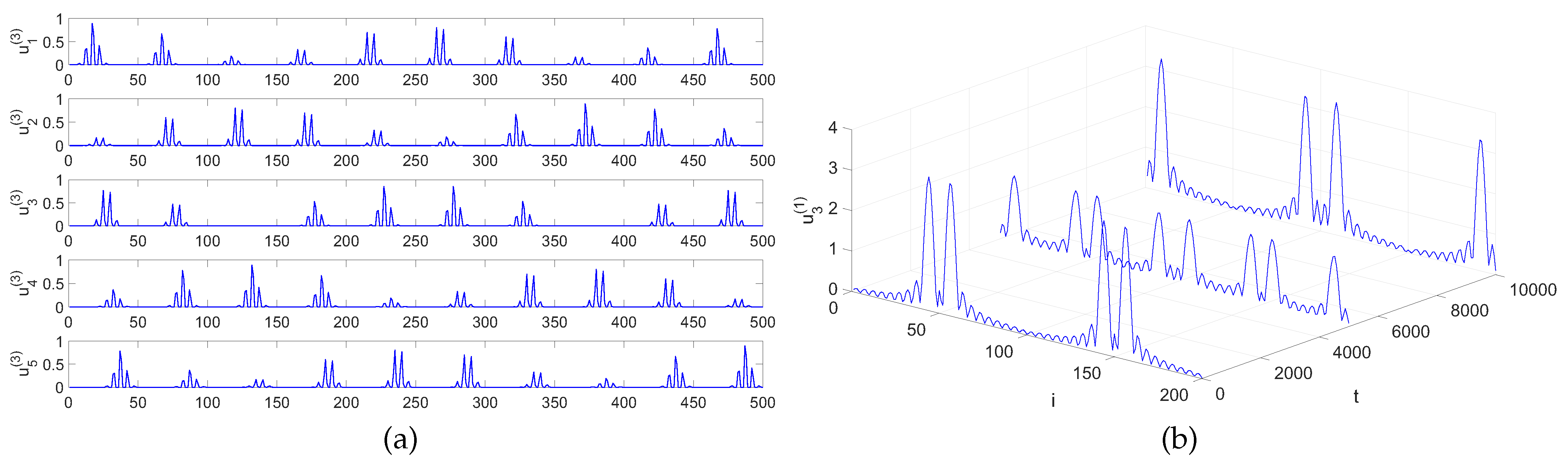
• Benchmark II: the observed dataset $\mathcal{Y}\in {\mathbb{R}}_{+}^{I_1\times I_2\times I_3}$ was also created using model (3). Factor matrices ${\mathit{U}}^{\left(1\right)}$ and ${\mathit{U}}^{\left(2\right)}$ were generated similarly as in Benchmark I. Each column in factor ${\mathit{U}}^{\left(3\right)}$ expresses the periodic Gaussian pulse train obtained by a repetition of Gaussian-modulated sinusoidal pulse, circularly shifted with a randomly selected time lag. The negative entries are replaced with a zero-value. One waveform of such a signal is plotted in Figure 1a. The frequency and the phase of the sinusoid signal was set individually for each component/column. Assuming ${\mathit{U}}^{\left(3\right)}$ represents source signals, the fibers in $\mathcal{Y}$ along the third mode can be regarded as mixed signals with a multi-linear mixing operator.
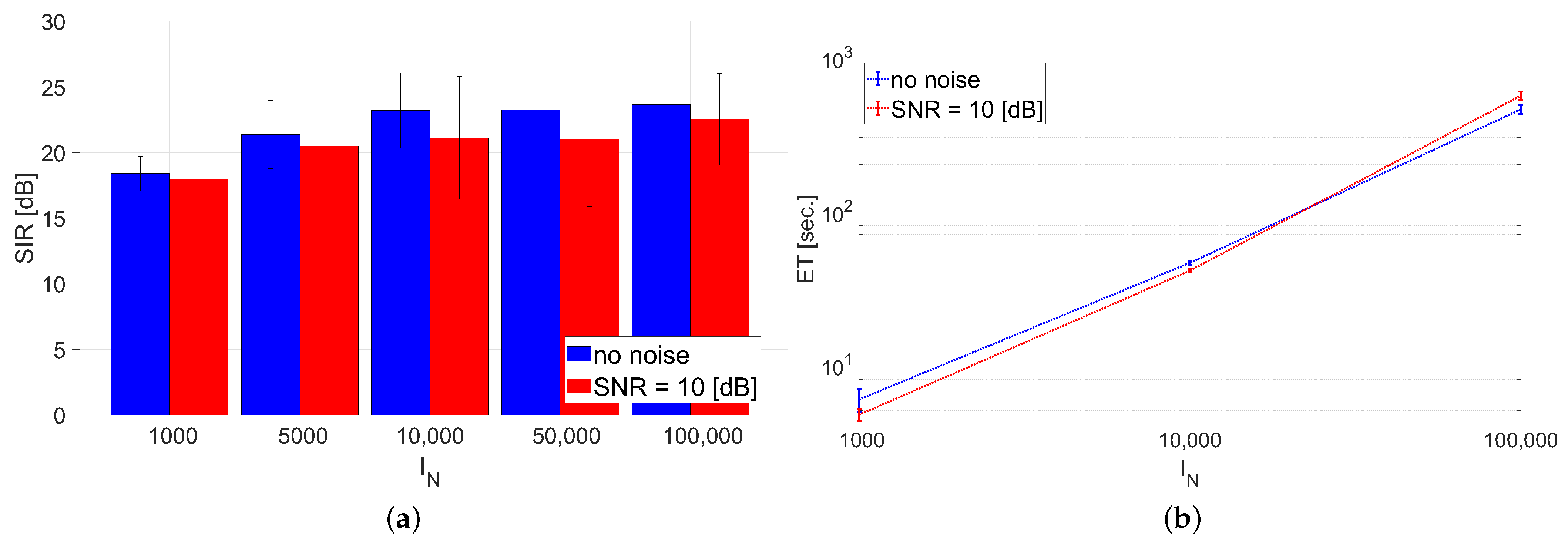
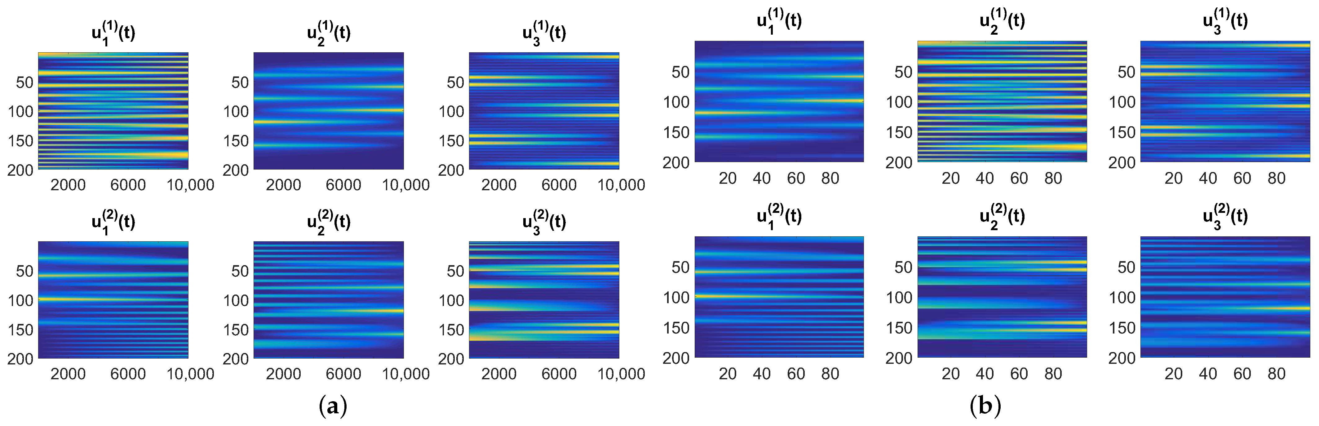
• Benchmark III: the observed dataset $\mathcal{Y}\in {\mathbb{R}}_{+}^{I_1\times I_2\times I_3}$ was created according to the dynamic NTD model in (38). For the whole set of temporal samples ($t=1,\dots ,T$), factors ${\mathit{U}}_t^{\left(1\right)}$ and ${\mathit{U}}_t^{\left(2\right)}$ take the form of three-way arrays ${\mathcal{U}}^{\left(1\right)}\in {\mathbb{R}}_{+}^{I_1\times J_1\times T}$ and ${\mathcal{U}}^{\left(2\right)}\in {\mathbb{R}}_{+}^{I_2\times J_2\times T}$ that contain $J_1$ and $J_2$ components, respectively. Each component is obtained by a linear interpolation of a pair of the spectral signals taken from the file AC10_art_spectr_noi in Matlab toolbox NMFLAB for Signal Processing [66]. Hence, $I_1$ and $I_2$ refer to spectral resolutions, while T denotes the number of time slots within the interpolated window. The example of one such component is illustrated in Figure 1b in the form of a 3D plot. Assuming the components in ${\mathcal{U}}^{\left(1\right)}$ and ${\mathcal{U}}^{\left(2\right)}$ are time-varying spectral signals, model (38) can be used to represent a time-varying multi-linear mixing process.

The proposed algorithms: BK-NTD (Algorithm 2) and RI-NTD (Algorithm 1) were compared with the HALS-NTD [67], which is regarded in the literature as one of the most efficient algorithms for NTD. The maximum number of iterations in the HALS-NTD was set to 100 and the tolerance for early termination was equal to ${10}^{-5}$. In the incremental versions of NTD, we set ${\tilde{I}}_3=100$ (the number of samples in an initial block) and $I_n^{\left(t\right)}=100$ (the number of samples in a regular block). The number of inner iterations in BK-NTD was set to 5, i.e., $K_i=5$. The maximum number of iterations in the NNLS algorithm both for BK-NTD as well as for RI-NTD was set to 300.

The BK-NTD and RI-NTD were implemented in MATLAB 2016b, and the HALS-NTD was taken from the Matlab toolbox TENSORBOX (https://faculty.skoltech.ru/people/anhhuyphan (accessed on 1 August 2018). All of the algorithms were run on a machine supplied with a 4-core Intel Core i7 CPU, 64 GB RAM, and an SSD drive.

To analyze the susceptibility of the algorithms to noisy perturbations, the synthetic data were perturbed with an additive zero-mean Gaussian noise $\mathcal{N}(0,{\sigma }^2)$ with the variance ${\sigma }^2$ selected to satisfy a given level of signal-to-noise ratio (SNR).

The following tests were performed using the above mentioned benchmarks:

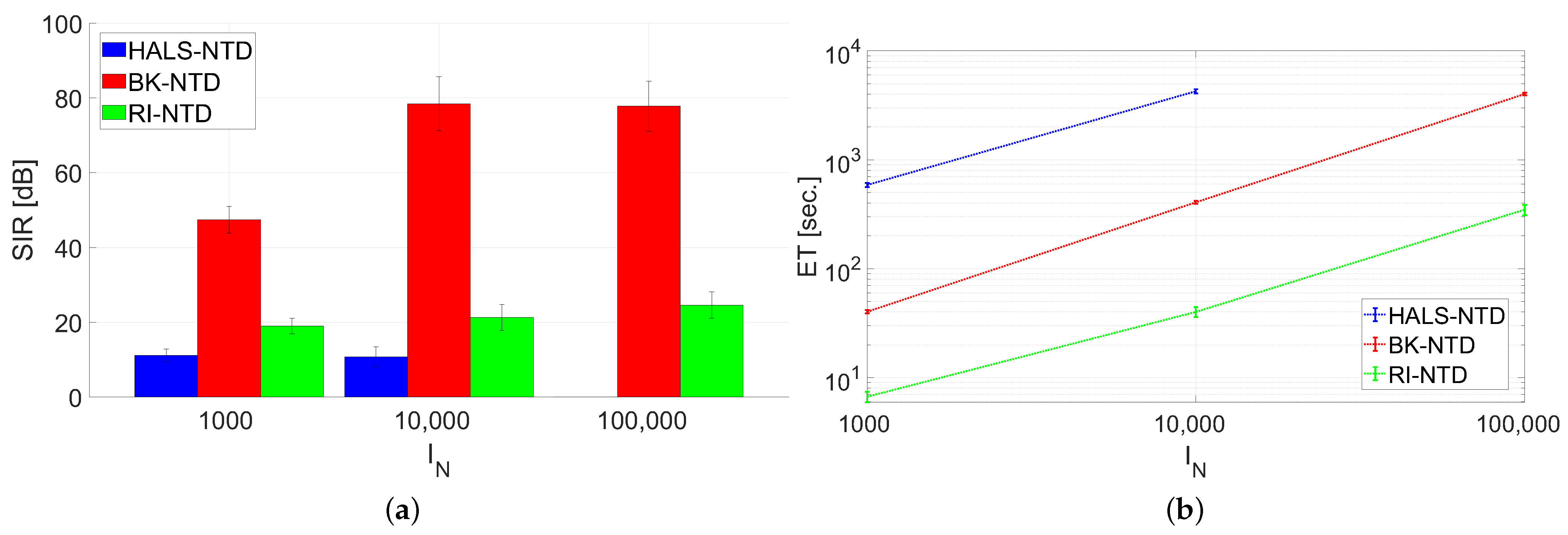
• Test A: Benchmark A was used in this test with settings: $I_1=I_2=100$ and $J_1=J_2=J_3=10$ in all the observed scenarios. The test was carried out for $I_3\in \{{10}^3,{10}^4,{10}^5\}$. No noisy perturbations were used in this test.
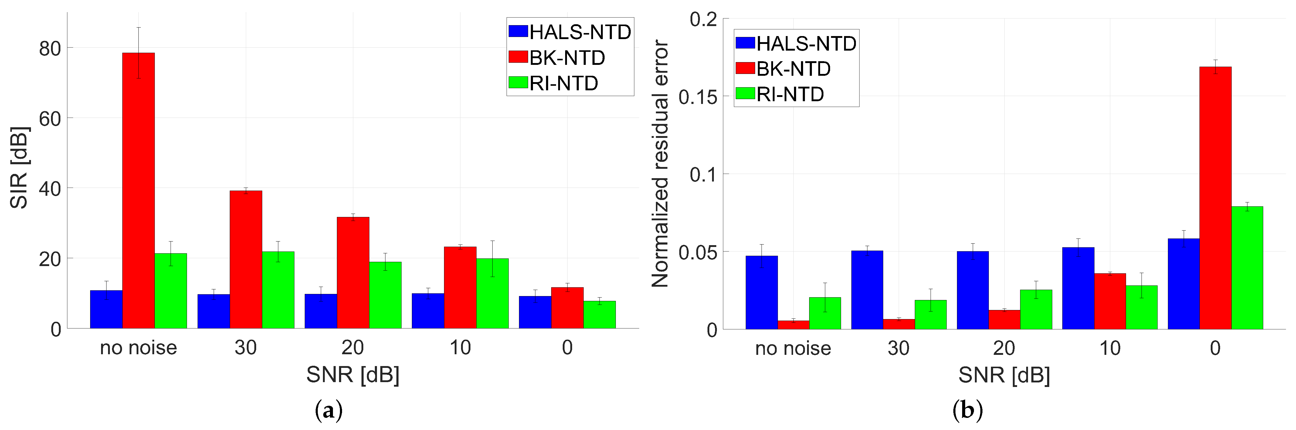
• Test B: Benchmark A was used in this test with settings: $I_1=I_2=100$, $I_3={10}^4$, and $J_1=J_2=J_3=10$ in all the observed scenarios. The synthetically generated data were additively perturbed with the zero-mean Gaussian noise with $\mathrm{SNR}\in \{30,20,10,0\}\left[\mathrm{dB}\right]$. Note that the noise with $\mathrm{SNR}=0\left[\mathrm{dB}\right]$ is very strong – the power of noise is equal to the power of the true signal.
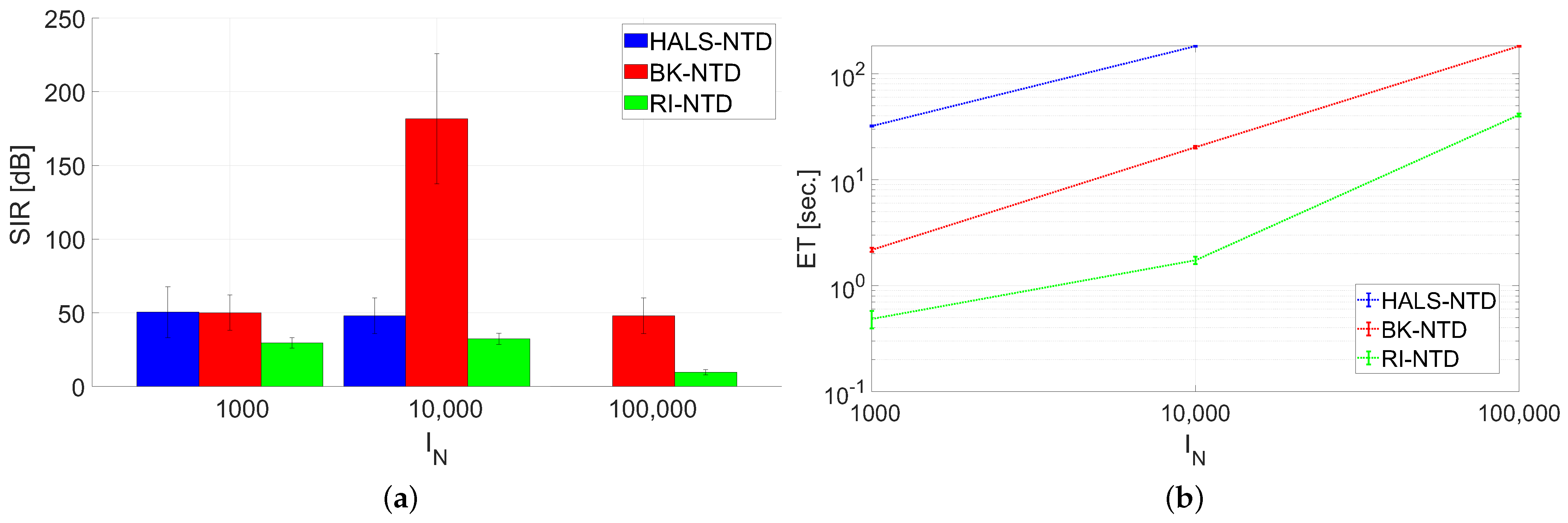
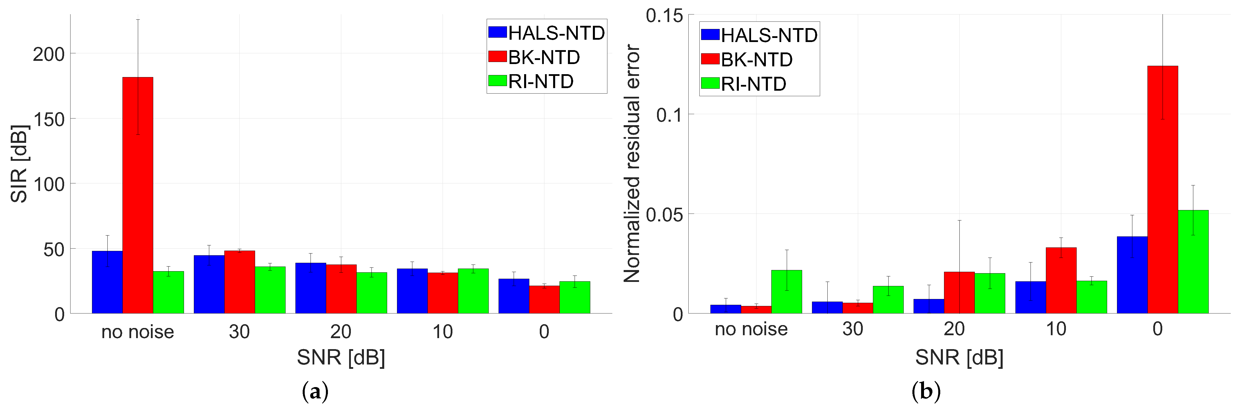
• Test C: Benchmark B was used in this test with settings: $I_1=I_2=50$ and $J_1=J_2=J_3=5$, and $I_3\in \{{10}^3,{10}^4,{10}^5\}$. No noisy perturbations were used in this test.
• Test D: Benchmark B was used in this test with settings: $I_1=I_2=50$, $I_3={10}^4$, and $J_1=J_2=J_3=5$ in all the observed scenarios. The synthetically generated data were additively perturbed with the zero-mean Gaussian noise with $\mathrm{SNR}\in \{30,20,10,0\}\left[\mathrm{dB}\right]$.
• Test E: Benchmark C was used in this test with settings: $I_1=I_2=200$ and $J_1=J_2=J_3=3$, and $I_3\in \{{10}^3,5\times {10}^3,{10}^4,5\times {10}^4,{10}^5\}$. Noise-free and noisy data with $\mathrm{SNR}=10\left[\mathrm{dB}\right]$ were tested.
  The algorithms were quantitatively evaluated in terms of the signal-to-interference ratio (SIR) measure [1], elapsed time (ET) of running (in seconds), and normalized residual error: ${\displaystyle r=\frac{\left|\right|\mathcal{Y}-\mathcal{G}{\times }_1{\mathbf{U}}^{\left(1\right)}{\times }_2\dots {\times }_N{\mathbf{U}}^{\left(N\right)}{\left|\right|}_F^2}{{\left|\right|\mathcal{Y}\left|\right|}_F}}$. Moreover, the selected estimated signals were also illustrated in the form of 2D plots.
  Since the optimization problem in the NTD model is non-convex and, hence, sensitive to initialization, we performed the Monte Carlo (MC) analysis with 10 runs. In each run, a new sample of dataset and a new initializer were randomly selected.

3.2. Results

Figure 2 presents the results obtained in Test A. The averaged SIR performance versus the length of the analyzed tensor with respect to the last mode (the third one) is illustrated in Figure 2a in the form of a bar plot. The standard deviation in the MC runs is marked with the whiskers. The averaged ET in Test A is illustrated in Figure 2b.

The results obtained in Test B are depicted in Figure 3. In this test, we demonstrate how the tested algorithms are prone to noisy perturbations. The averaged SIR performance and the normalized residual error versus the power of noisy disturbances are illustrated in Figure 3a,b, respectively. Figure 4a,b present the averaged SIR values and the ET versus the number of observed samples ($I_3$) in Test C, respectively. Figure 5a illustrates the averaged SIR performance versus the SNR values. The corresponding normalized residual errors are depicted in Figure 5b.

Figure 6 and Figure 7 show the results obtained in Test E in which only BK-NTD was used, but in the online version expressed by model (38). In this case, the SIR was computed for ${\mathit{U}}^{\left(3\right)}$ and the last samples in ${\mathit{U}}^{\left(1\right)}$ and ${\mathit{U}}^{\left(2\right)}$ since the temporal resolution decreases with respect to the original factors (due to sequential batch processing). The SIR performance versus the number of entries along the third mode is illustrated in Figure 6a for noise-free and noisy data. The corresponding averaged ET values are presented in Figure 6b.

The original and estimated spectral signals that are represented by factors ${\mathit{U}}^{\left(1\right)}$ and ${\mathit{U}}^{\left(2\right)}$ are displayed in Figure 7 in the form of 2D plots with scaled colors. Note that ${\mathit{u}}_3^{\left(1\right)}\left(t\right)$ in Figure 7a presents the same signal as shown in Figure 1b, but in a more compact and informative way, especially for subjective evaluation of time-varying peak profiles.

3.3. Discussion

The results demonstrate multiple advantages of the proposed incremental versions of NTD. First, these methods are much faster than batch processing, especially when the observed data contain large numbers of samples. Figure 2b and Figure 4b show that BK-NTD is at least 10 times faster than HALS-NTD, and RI-NTD is about 10 times faster than BK-NTD. The computational complexities of the proposed methods increase linearly with $I_N$, and the experimental results confirm the theoretical analyses in Remarks 1, 2, and 3. Second, the high speed of processing is neither obtained due to a decrease in the quality of model fitting nor the SIR performance. On the contrary, BK-NTD and RI-NTD in Tests A and B (Figure 2 and Figure 3) have considerably higher SIR performance than HALS-NTD if $\mathrm{SNR}\ge 10\left[\mathrm{dB}\right]$, at a significantly lower level of the residual error. For a very strong noise ($\mathrm{SNR}=0\left[\mathrm{dB}\right]$) all algorithms have a similar SIR performance, but HALS-NTD reaches a lower residual error.

Benchmark II is more difficult for the proposed algorithms than Benchmark I. However, BK-NTD considerably outperforms HALS-NTD for noise-free data with $I_N={10}^4$, as demonstrated in Test C. For other test cases (in Test C and D), there is no significant difference in the SIR performance between BK-NTD and HALS-NTD. RI-NTD yields the factors of a similar quality as the other algorithms, but only for strongly noisy data ($\mathrm{SNR}\le 10\left[\mathrm{dB}\right]$). Comparing RI-NTD with BK-NTD, we observed that the former is much faster, but has a better SIR performance only for very noisy data from Benchmark II.

The next advantage of the proposed algorithms is that they can process nearly an infinitely long sequence of multi-way samples, which is intractable for batch NTD algorithms, e.g., such as HALS-NTD. We were unable to run HALS-NTD when $I_3={10}^5$ due to the limit of RAM memory (we used 64 GB RAM), while the limit for the incremental versions of NTD restricts mostly to processing time in practice. Due to the incremental processing of multi-way data, factors ${\mathit{U}}^{\left(1\right)}$ and ${\mathit{U}}^{\left(2\right)}$ can capture a dynamic characteristics of the underlying processes. In other words, the factors can vary with time or along with the mode representing the samples. The results obtained in Test E confirmed that BK-NTD demonstrates a high efficiency in recovering dynamic factors ${\mathit{U}}^{\left(1\right)}$ and ${\mathit{U}}^{\left(2\right)}$, even for strongly noisy data. As shown in Figure 6a, the difference in the SIR performance between the noise-free and noisy data with $\mathrm{SNR}=10\left[\mathrm{dB}\right]$ is statistically not significant. The quality of estimation depends on the length of an input sequence but the SIR performance weakly changes if the sequences are not shorter than ${10}^4$ samples (see Figure 6a). The quality of the estimated factors can also be confirmed by the results shown in Figure 7. Similarly as in Tests A and B, the time complexity is linear in terms of the number of samples, which is confirmed by the results plotted in Figure 6b.

4. Conclusions

In this study, we proposed new computational algorithms for an incremental version of the NTD model. One of them is based on the concept of row-action projections with the block Kaczmarz method, and the other uses the recursive nonnegative least-squares updates. The algorithms were applied both for performing the NTD of a long sequence of multi-way samples as well as for extracting time-varying multi-linear features. All of the proposed solutions were validated experimentally with respect to multiple benchmarks and criteria, including the quality of estimated factors and the runtime. The numerical results demonstrated that both algorithms are at least ten times faster than the batch version of NTD (HALS-NTD), keeping at least the same quality of estimated factors. In a few test cases, the block Kaczmarz algorithm considerably outperforms the baseline version of NTF with respect to the quality of the estimated factors and the residual error, even for moderately noisy data. The block Kaczmarz method also demonstrated a high efficiency in processing a dynamic NTD model with all of the time-varying estimated factors. This approach can find a number of potential applications, e.g., for solving a blind source separation problem with a time-varying mixing operator or for a spectral signal unmixing problem with dynamic endmember spectra.

To summarize, we proposed efficient computational approaches for incremental processing of a long sequence of multi-way samples with the NTD model and for estimating time-varying features in the dynamic NTD model. The efficiency is confirmed with multiple experimental results. Obviously, the proposed methodology can be extended in the future, e.g., to tackle partially orthogonal time-varying features or as an extension to other tensor decomposition models, such as tensor networks.

References

1. Cichocki, A.; Zdunek, R.; Phan, A.H.; Amari, S.I. Nonnegative Matrix and Tensor Factorizations: Applications to Exploratory Multi-Way Data Analysis and Blind Source Separation; Wiley and Sons: Chichester, UK, 2009. [Google Scholar]
2. Kisil, I.; Calvi, G.G.; Scalzo Dees, B.; Mandic, D.P. Tensor Decompositions and Practical Applications: A Hands-on Tutorial. In Recent Trends in Learning From Data: Tutorials from the INNS Big Data and Deep Learning Conference (INNSBDDL2019); Oneto, L., Navarin, N., Sperduti, A., Anguita, D., Eds.; Springer International Publishing: Cham, Switzerland, 2020; pp. 69–97. [Google Scholar]
3. Carroll, J.D.; Chang, J.J. Analysis of individual differences in multidimensional scaling via an n-way generalization of Eckart-Young decomposition. Psychometrika 1970, 35, 283–319. [Google Scholar] [CrossRef]
4. Harshman, R.A. Foundations of the PARAFAC procedure: Models and conditions for an “explanatory”multimodal factor analysis. UCLA Work. Pap. Phon. 1970, 16, 1–84. [Google Scholar]
5. Lim, L.H.; Comon, P. Nonnegative approximations of nonnegative tensors. J. Chemom. 2009, 23, 432–441. [Google Scholar] [CrossRef] [Green Version]
6. Wang, D.; Cong, F.; Ristaniemi, T. Sparse Nonnegative CANDECOMP/PARAFAC Decomposition in Block Coordinate Descent Framework: A Comparison Study. arXiv 2018, arXiv:abs/1812.10637. [Google Scholar]
7. Alexandrov, B.S.; DeSantis, D.; Manzini, G.; Skau, E.W. Nonnegative Canonical Polyadic Decomposition with Rank Deficient Factors. arXiv 2019, arXiv:abs/1909.07570. [Google Scholar]
8. Tucker, L.R. The extension of factor analysis to three-dimensional matrices. In Contributions to Mathematical Psychology; Gulliksen, H., Frederiksen, N., Eds.; Holt, Rinehart and Winston: New York, NY, USA, 1964; pp. 110–127. [Google Scholar]
9. Tucker, L.R. Some mathematical notes on three-mode factor analysis. Psychometrika 1966, 31, 279–311. [Google Scholar] [CrossRef]
10. Mørup, M.; Hansen, L.K.; Arnfred, S.M. Algorithms for Sparse Nonnegative Tucker Decompositions. Neural Comput. 2008, 20, 2112–2131. [Google Scholar] [CrossRef]
11. Oh, S.; Park, N.; Lee, S.; Kang, U. Scalable Tucker Factorization for Sparse Tensors—Algorithms and Discoveries. In Proceedings of the 34th IEEE International Conference on Data Engineering (ICDE), Paris, France, 16–19 April 2018; pp. 1120–1131. [Google Scholar]
12. De Lathauwer, L.; de Moor, B.; Vandewalle, J. A multilinear singular value decomposition. SIAM J. Matrix Anal. Appl. 2000, 21, 1253–1278. [Google Scholar] [CrossRef] [Green Version]
13. Sheehan, B.N.; Saad, Y. Higher Order Orthogonal Iteration of Tensors (HOOI) and its Relation to PCA and GLRAM. In Proceedings of the Seventh SIAM International Conference on Data Mining, Minneapolis, MN, USA, 26–28 April 2007; pp. 355–365. [Google Scholar]
14. Hackbusch, W.; Kühn, S. A New Scheme for the Tensor Representation. J. Fourier Anal. Appl. 2009, 15, 706–722. [Google Scholar] [CrossRef] [Green Version]
15. Oseledets, I.V. Tensor-Train Decomposition. SIAM J. Sci. Comput. 2011, 33, 2295–2317. [Google Scholar] [CrossRef]
16. Cichocki, A.; Lee, N.; Oseledets, I.V.; Phan, A.H.; Zhao, Q.; Mandic, D.P. Tensor Networks for Dimensionality Reduction and Large-scale Optimization: Part 1 Low-Rank Tensor Decompositions. Found. Trends Mach. Learn. 2016, 9, 249–429. [Google Scholar] [CrossRef] [Green Version]
17. Cichocki, A.; Phan, A.H.; Zhao, Q.; Lee, N.; Oseledets, I.V.; Sugiyama, M.; Mandic, D.P. Tensor Networks for Dimensionality Reduction and Large-scale Optimization: Part 2 Applications and Future Perspectives. Found. Trends Mach. Learn. 2017, 9, 431–673. [Google Scholar] [CrossRef]
18. Zhao, Q.; Zhou, G.; Xie, S.; Zhang, L.; Cichocki, A. Tensor Ring Decomposition. arXiv 2016, arXiv:1606.05535. [Google Scholar]
19. Liu, J.; Zhu, C.; Liu, Y. Smooth Compact Tensor Ring Regression. IEEE Trans. Knowl. Data Eng. 2020. [Google Scholar] [CrossRef]
20. Vasilescu, M.A.O.; Terzopoulos, D. Multilinear analysis of image ensembles: Tensorfaces. In European Conf. on Computer Vision (ECCV); Springer: Berlin/Heidelberg, Germany, 2002; Volume 2350, pp. 447–460. [Google Scholar]
21. Wang, H.; Ahuja, N. Facial Expression Decomposition. In Proceedings of the Ninth IEEE International Conference on Computer Vision, Nice, France, 13–16 October 2003; Volume 2, pp. 958–965. [Google Scholar]
22. Vlasic, D.; Brand, M.; Phister, H.; Popovic, J. Face transfer with multilinear models. ACM Trans. Graph. 2005, 24, 426–433. [Google Scholar] [CrossRef]
23. Zhang, M.; Ding, C. Robust Tucker Tensor Decomposition for Effective Image Representation. In Proceedings of the 2013 IEEE International Conference on Computer Vision, Sydney, Australia, 1–8 December 2013; pp. 2448–2455. [Google Scholar]
24. Zaoralek, L.; Prilepok, M.; Snael, V. Recognition of Face Images with Noise Based on Tucker Decomposition. In Proceedings of the 2015 IEEE International Conference on Systems, Man, and Cybernetics, Hong Kong, China, 9–12 October 2015; pp. 2649–2653. [Google Scholar]
25. Savas, B.; Elden, L. Handwritten digit classification using higher order singular value decomposition. Pattern Recognit. 2007, 40, 993–1003. [Google Scholar] [CrossRef]
26. Phan, A.H.; Cichocki, A. Tensor decompositions for feature extraction and classification of high dimensional datasets. IEICE Nonlinear Theory Its Appl. 2010, 1, 37–68. [Google Scholar] [CrossRef] [Green Version]
27. Phan, A.H.; Cichocki, A.; Vu-Dinh, T. Classification of Scenes Based on Multiway Feature Extraction. In Proceedings of the 2010 International Conference on Advanced Technologies for Communications, Ho Chi Minh City, Vietnam, 20–22 October 2010; pp. 142–145. [Google Scholar]
28. Araujo, D.C.; de Almeida, A.L.F.; Da Costa, J.P.C.L.; de Sousa, R.T. Tensor-Based Channel Estimation for Massive MIMO-OFDM Systems. IEEE Access 2019, 7, 42133–42147. [Google Scholar] [CrossRef]
29. Sun, Y.; Gao, J.; Hong, X.; Mishra, B.; Yin, B. Heterogeneous Tensor Decomposition for Clustering via Manifold Optimization. IEEE Trans. Pattern Anal. Mach. Intell. 2016, 38, 476–489. [Google Scholar] [CrossRef] [PubMed] [Green Version]
30. Chen, H.; Ahmad, F.; Vorobyov, S.; Porikli, F. Tensor Decompositions in Wireless Communications and MIMO Radar. IEEE J. Sel. Top. Signal Process. 2021, 15, 438–453. [Google Scholar] [CrossRef]
31. Li, R.; Pan, Z.; Wang, Y.; Wang, P. The correlation-based Tucker decomposition for hyperspectral image compression. Neurocomputing 2021, 419, 357–370. [Google Scholar] [CrossRef]
32. Ebied, A.; Kinney-Lang, E.; Spyrou, L.; Escudero, J. Muscle Activity Analysis Using Higher-Order Tensor Decomposition: Application to Muscle Synergy Extraction. IEEE Access 2019, 7, 27257–27271. [Google Scholar] [CrossRef]
33. Kolda, T.G.; Bader, B.W. Tensor Decompositions and Applications. SIAM Rev. 2009, 51, 455–500. [Google Scholar] [CrossRef]
34. Rabanser, S.; Shchur, O.; Günnemann, S. Introduction to Tensor Decompositions and their Applications in Machine Learning. arXiv 2017, arXiv:1711.10781. [Google Scholar]
35. Kim, Y.D.; Choi, S. Nonnegative Tucker Decomposition. In Proceedings of the IEEE Conference on Computer Vision and Pattern Recognition (CVPR07), Minneapolis, MN, USA, 17–22 June 2007; pp. 1–8. [Google Scholar]
36. Li, X.; Ng, M.K.; Cong, G.; Ye, Y.; Wu, Q. MR-NTD: Manifold Regularization Nonnegative Tucker Decomposition for Tensor Data Dimension Reduction and Representation. IEEE Trans. Neural Netw. Learn. Syst. 2017, 28, 1787–1800. [Google Scholar] [CrossRef] [PubMed]
37. Zhou, G.; Cichocki, A.; Zhao, Q.; Xie, S. Efficient Nonnegative Tucker Decompositions: Algorithms and Uniqueness. IEEE Trans. Image Process. 2015, 24, 4990–5003. [Google Scholar] [CrossRef] [PubMed] [Green Version]
38. Qiu, Y.; Zhou, G.; Zhang, Y.; Xie, S. Graph Regularized Nonnegative Tucker Decomposition for Tensor Data Representation. In Proceedings of the 2019 IEEE International Conference on Acoustics, Speech and Signal Processing (ICASSP), Brighton, UK, 12–17 May 2019; pp. 8613–8617. [Google Scholar]
39. Qiu, Y.; Zhou, G.; Wang, Y.; Zhang, Y.; Xie, S. A Generalized Graph Regularized Non-Negative Tucker Decomposition Framework for Tensor Data Representation. IEEE Trans. Cybern. 2020; 1–14, in press. [Google Scholar] [CrossRef]
40. Bai, X.; Xu, F.; Zhou, L.; Xing, Y.; Bai, L.; Zhou, J. Nonlocal Similarity Based Nonnegative Tucker Decomposition for Hyperspectral Image Denoising. IEEE J. Sel. Top. Appl. Earth Obs. Remote Sens. 2018, 11, 701–712. [Google Scholar] [CrossRef] [Green Version]
41. Li, J.; Liu, Z. Compression of hyper-spectral images using an accelerated nonnegative tensor decomposition. Open Phys. 2017, 15, 992–996. [Google Scholar] [CrossRef] [Green Version]
42. Marmoret, A.; Cohen, J.E.; Bertin, N.; Bimbot, F. Uncovering audio patterns in music with Nonnegative Tucker Decomposition for structural segmentation. arXiv 2021, arXiv:2104.08580. [Google Scholar]
43. Zare, M.; Helfroush, M.S.; Kazemi, K.; Scheunders, P. Hyperspectral and Multispectral Image Fusion Using Coupled Non-Negative Tucker Tensor Decomposition. Remote Sens. 2021, 13, 2930. [Google Scholar] [CrossRef]
44. Anh-Dao, N.T.; Le Thanh, T.; Linh-Trung, N.; Vu Le, H. Nonnegative Tensor Decomposition for EEG Epileptic Spike Detection. In Proceedings of the 2018 5th NAFOSTED Conference on Information and Computer Science (NICS), Ho Chi Minh City, Vietnam, 23–24 November 2018; pp. 194–199. [Google Scholar]
45. Rostakova, Z.; Rosipal, R.; Seifpour, S.; Trejo, L.J. A Comparison of Non-negative Tucker Decomposition and Parallel Factor Analysis for Identification and Measurement of Human EEG Rhythms. Meas. Sci. Rev. 2020, 20, 126–138. [Google Scholar] [CrossRef]
46. Sidiropoulos, N.; De Lathauwer, L.; Fu, X.; Huang, K.; Papalexakis, E.; Faloutsos, C. Tensor Decomposition for Signal Processing and Machine Learning. IEEE Trans. Acoust. Speech Signal Process. 2017, 65, 3551–3582. [Google Scholar] [CrossRef]
47. Bjorck, A. Numerical Methods for Least Squares Problems; SIAM: Philadelphia, PA, USA, 1996. [Google Scholar]
48. Zdunek, R.; Kotyla, M. Extraction of Dynamic Nonnegative Features from Multidimensional Nonstationary Signals. In Proceedings of the Data Mining and Big Data, First International Conference, Bali, Indonesia, 25–30 June 2016; Tan, Y., Shi, Y., Eds.; Springer: Berlin, Germany, 2016. Lecture Notes in Computer Science. Volume 9714, pp. 557–566. [Google Scholar]
49. Xiao, H.; Wang, F.; Ma, F.; Gao, J. eOTD: An Efficient Online Tucker Decomposition for Higher Order Tensors. In Proceedings of the 2018 IEEE International Conference on Data Mining (ICDM), Singapore, 17–20 November 2018; pp. 1326–1331. [Google Scholar]
50. Needell, D.; Tropp, J.A. Paved with good intentions: Analysis of a randomized block Kaczmarz method. Linear Algebra Its Appl. 2014, 441, 199–221. [Google Scholar] [CrossRef] [Green Version]
51. Needell, D.; Zhao, R.; Zouzias, A. Randomized block Kaczmarz method with projection for solving least squares. Linear Algebra Its Appl. 2015, 484, 322–343. [Google Scholar] [CrossRef]
52. Zhou, S.; Erfani, S.M.; Bailey, J. Online CP Decomposition for Sparse Tensors. In Proceedings of the 2018 IEEE International Conference on Data Mining (ICDM), Singapore, 17–20 November 2018; pp. 1458–1463. [Google Scholar]
53. Zeng, C.; Ng, M.K. Incremental CP Tensor Decomposition by Alternating Minimization Method. SIAM J. Matrix Anal. Appl. 2021, 42, 832–858. [Google Scholar] [CrossRef]
54. Liu, H.; Yang, L.T.; Guo, Y.; Xie, X.; Ma, J. An Incremental Tensor-Train Decomposition for Cyber-Physical-Social Big Data. IEEE Trans. Big Data 2021, 7, 341–354. [Google Scholar] [CrossRef]
55. Lubich, C.; Rohwedder, T.; Schneider, R.; Vandereycken, B. Dynamical Approximation by Hierarchical Tucker and Tensor-Train Tensors. SIAM J. Matrix Anal. Appl. 2013, 34, 470–494. [Google Scholar] [CrossRef] [Green Version]
56. Sun, J.; Tao, D.; Faloutsos, C. Beyond streams and graphs: Dynamic tensor analysis. In Proceedings of the 12th ACM SIGKDD International Conference on Knowledge Discovery and Data Mining, Philadelphia, PA, USA, 20–23 August 2006. [Google Scholar]
57. Sun, J.; Papadimitriou, S.; Yu, P.S. Window-based Tensor Analysis on High-dimensional and Multi-aspect Streams. In Proceedings of the Sixth International Conference on Data Mining, Hong Kong, China, 18–22 December 2006; pp. 1076–1080. [Google Scholar]
58. Sun, J.; Tao, D.; Papadimitriou, S.; Yu, P.S.; Faloutsos, C. Incremental tensor analysis: Theory and applications. ACM Trans. Knowl. Discov. Data 2008, 2, 11:1–11:37. [Google Scholar] [CrossRef]
59. Fanaee-T, H.; Gama, J. Multi-aspect-streaming tensor analysis. Knowl. Based Syst. 2015, 89, 332–345. [Google Scholar] [CrossRef] [Green Version]
60. Gujral, E.; Pasricha, R.; Papalexakis, E.E. SamBaTen: Sampling-based Batch Incremental Tensor Decomposition. In Proceedings of the 2018 SIAM International Conference on Data Mining, San Diego Marriott Mission Valley, San Diego, CA, USA, 3–5 May 2018; pp. 387–395. [Google Scholar]
61. Malik, O.A.; Becker, S. Low-Rank Tucker Decomposition of Large Tensors Using TensorSketch. In Proceedings of the Advances in Neural Information Processing Systems, Montreal, QC, Canada, 2–8 December 2018; Volume 31. [Google Scholar]
62. Traore, A.; Berar, M.; Rakotomamonjy, A. Online multimodal dictionary learning through Tucker decomposition. Neurocomputing 2019, 368, 163–179. [Google Scholar] [CrossRef] [Green Version]
63. Fang, S.; Kirby, R.M.; Zhe, S. Bayesian streaming sparse Tucker decomposition. In Proceedings of the Thirty-Seventh Conference on Uncertainty in Artificial Intelligence, Toronto, QC, Canada, 26–30 July 2021; Volume 161, pp. 558–567. [Google Scholar]
64. Sobral, A.; Javed, S.; Ki Jung, S.; Bouwmans, T.; Zahzah, E.h. Online Stochastic Tensor Decomposition for Background Subtraction in Multispectral Video Sequences. In Proceedings of the IEEE International Conference on Computer Vision (ICCV) Workshops, Santiago, Chile, 7–13 December 2015. [Google Scholar]
65. Chachlakis, D.G.; Dhanaraj, M.; Prater-Bennette, A.; Markopoulos, P.P. Dynamic L1-Norm Tucker Tensor Decomposition. IEEE J. Sel. Top. Signal Process. 2021, 15, 587–602. [Google Scholar] [CrossRef]
66. Cichocki, A.; Zdunek, R. NMFLAB for Signal and Image Processing; Technical Report; Laboratory for Advanced Brain Signal Processing, BSI, RIKEN: Saitama, Japan, 2006. [Google Scholar]
67. Phan, A.H.; Cichocki, A. Extended HALS algorithm for nonnegative Tucker decomposition and its applications for multiway analysis and classification. Neurocomputing 2011, 74, 1956–1969. [Google Scholar] [CrossRef]
Figure 1. Original signals: (a) 500 samples of 5 source signals used to generate U ( 3 ) in Test B, (b) one exemplary time-varying component from U ( 1 ) used to generate the observed data in Test C.
Symmetry 14 00113 g001
Figure 2. Results obtained in Test A: (a) SIR performance versus the number of entries along the third mode ( I N ), (b) elapsed time versus the number of entries along the third mode ( I N ).
Symmetry 14 00113 g002
Figure 3. Results obtained in Test B: (a) SIR performance versus SNR values, (b) normalized residual error versus SNR values.
Symmetry 14 00113 g003
Figure 4. Results obtained in Test C: (a) SIR performance versus the number of entries along the third mode ( I N ), (b) elapsed time versus the number of entries along the third mode ( I N ).
Symmetry 14 00113 g004
Figure 5. Results obtained in Test D: (a) SIR performance versus SNR values, (b) normalized residual error versus SNR values.
Symmetry 14 00113 g005
Figure 6. Results obtained in Test E (only BK-NTD algorithm): (a) SIR performance versus the number of entries along the third mode ( I N ), (b) elapsed time versus the number of entries along the third mode ( I N ).
Symmetry 14 00113 g006
Figure 7. Results obtained in Test E (only BK-NTD algorithm) presented in the form of 2D color images (90 degrees viewpoint): (a) original spectral signals used to generate factors U ( 1 ) R + 200 × 3 × 10000 and U ( 2 ) R + 200 × 3 × 10000 , (b) estimated spectral signals obtained from factors U ( 1 ) R + 200 × 3 × 100 and U ( 2 ) R + 200 × 3 × 100 with the following SIR values for the subsequent components from U ( 1 ) : 19.33, 23.21, 27.35 [dB], and 25.34, 39.42, 27.54 [dB] for U ( 2 ) ( I 3 = 10 4 and noise-free data).
Symmetry 14 00113 g007
Publisher’s Note: MDPI stays neutral with regard to jurisdictional claims in published maps and institutional affiliations.