On a Surface Associated with Pascal’s Triangle

Abstract

An open problem in reliability theory is that of finding all the coefficients of the reliability polynomial associated with particular networks. Because reliability polynomials can be expressed in Bernstein form (hence linked to binomial coefficients), it is clear that an extension of the classical discrete Pascal’s triangle (comprising all the binomial coefficients) to a continuous version (exhibiting infinitely many values in between the binomial coefficients) might be geometrically helpful and revealing. That is why we have decided to investigate the geometric properties of a continuous extension of Pascal’s triangle including: Gauss curvatures, mean curvatures, geodesics, and level curves, as well as their symmetries.

1. Introduction

We have been working on circuit reliability for quite some time, see [1,2,3]. As such, digital system reliability is a field established in the 1950s by John von Neumann, who approached it from the gate level [4]. Around the same time, Edward F. Moore and Claude E. Shannon considered an alternate viewpoint and started from the lower device level [5,6]. Lately, the relentless scaling of CMOS transistors [7] has been the driving force calling for reliability enhancements of complex digital systems affected by noises and variations [8,9]. These have inspired us to investigate consecutive systems [10,11] and, more recently, hammocks [12], as well as other particular two-terminal networks [13].

Obviously, over time we had to become familiar with reliability polynomials and have realized that representing these polynomials in Bernstein form [14] is convenient as the associated coefficients have special meanings [15,16], but also as they might allow for easier comparisons and ranking of networks [13,17]. For an in-depth view, we refer the interested reader to the following two fresh surveys [18,19]. About four years ago, we realized that Bernstein polynomials, having coefficients that are a fraction of the binomial coefficients, could be mapped onto, or should we say in between, the binomial coefficients of the classical (discrete) Pascal’s triangle. That is why we started looking at extensions of Pascal’s triangle to real numbers, our expectations being that the coefficients of Bernstein reliability polynomials for “optimal” networks might correspond to particular geodesics on a continuous Pascal’s triangle or at least be correlated to some other geometrical properties.

This paper will start by presenting the state-of-the-art of Pascal’s triangle and follow with its extensions to real and complex numbers in Section 2. Afterwards, we shall focus on studying the surface represented by the continuous extension of the classical Pascal’s triangle (Pascal’s Surface) for positive real numbers, in Section 3. These will be followed by Discussion and Conclusions, including future directions for research.

2. State-of-the-Art

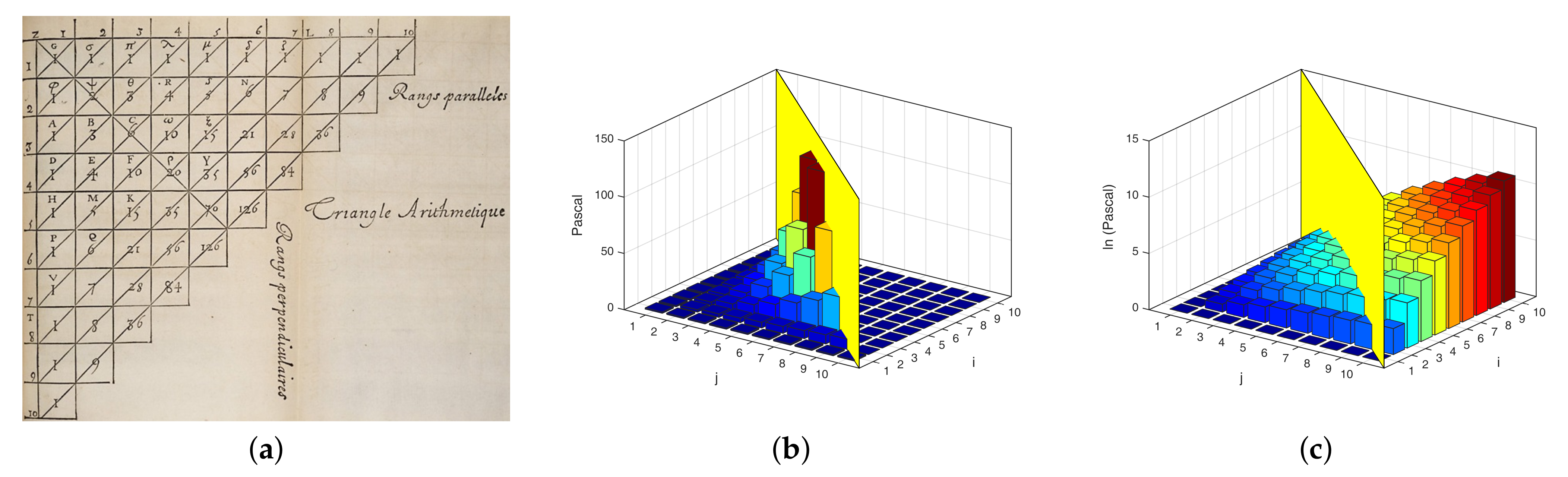
2.1. Pascal’s Triangle

Probably the most famous triangular arrangement of integers is the one containing the coefficients of the binomial expansion of ${\left(x+y\right)}^n$. It is known as Pascal’s triangle, although the triangle itself has been known and studied many centuries earlier by other mathematicians in India (Acharya Pingala 3rd/2nd century B.C.), Halayudha (c. 10th century), the Arab world and Persia (Al-Karaji (953–1029) and Omar Khayyam (1048–1131)), China (Jia Xian (1010–1070), Yang Hui (1238–1298), and Zhu Shijie (1249–1314)), as well as Europe (Ramon Llull (1232–1316), Michael Stifel (1487–1567), Petrus Apianus (1495–1552), Niccolo Tartaglia (1499–1557), and Marin Mersenne (1588–1648)). Still, Pascal proved several important properties of the binomial coefficients, and wrote the first modern treatise regarding this arithmetical triangle ([20]).

It seems that Blaise Pascal became aware of this arithmetical triangle for the first time when still in his teens, during a visit to Mersenne. In 1636, Father Mersenne published a large arithmetical triangle in Harmonicorum Libri XII (he wanted to apply the knowledge of combinatorics to musical theory). Almost two decades later, in 1654, Pascal wrote Traité du Triangle Arithmétique [20], which was not printed until 1665 (after Pascal’s death). Among other aspects, it details 19 properties (Pascal called them Consequences) of the binomial coefficients that could be derived from this arithmetic triangle. Some of the most important identities are represented by Consequences V and VIII, which currently can be found in any high school math curriculum.

The first mathematician who named the triangle after Pascal was Pierre Raymond de Montmort in 1708, who called it “Table de M. Pascal pour les combinaisons”. Around 1730, Abraham de Moivre called it “Triangulum Arithmeticum Pascalianum”, and this name has stuck with Western scientists, while being called Khayyam’s triangle in Iran, and Yang Hui’s triangle in China. It should be mentioned that, using Pascal’s triangle, one can derive and investigate many notable sequences of integers, e.g., Fibonacci, Catalan, Lucas, Bernoulli, and Stirling numbers. Moreover, if all the positions containing odd numbers are colored black and all the positions containing even numbers are colored white, the Sierpinski triangle is obtained. For additional properties and identities, the interested reader is referred to [21,22,23].

Over time, Pascal’s triangle has been represented in more than one form. In the following, two of these forms are shown to be related through a simple matrix identity [24]. Consider $P(\infty )$ the infinite symmetric matrix of components $P{(\infty )}_{i,j}=\left(\genfrac{}{}{0pt}{}{i+j}{i}\right)$, for $i,j\ge 1$ (the rows and columns of the matrix are indexed by positive integers):

$$P(\infty )=\left(\begin{array}{ccccccc}1& 1& 1& 1& 1& 1& ...\\ 1& 2& 3& 4& 5& 6& ...\\ 1& 3& 6& 10& 15& 21& ...\\ 1& 4& 10& 20& 35& 56& ...\\ 1& 5& 15& 35& 70& 126& ...\\ 1& 6& 21& 56& 126& 252& ...\\ ⋮& ⋮& ⋮& ⋮& ⋮& ⋮& \ddots \end{array}\right).$$

(1)

From Figure 1a (a scan provided by Cambridge University Library on Wikipedia, https://commons.wikimedia.org/wiki/File:TrianguloPascal.jpg, accessed on 6 February 2022), it can be seen that $P(\infty )$ is a perfect match of the form described by Pascal. Direct computation shows that

$$P(\infty )=L(\infty )·L{(\infty )}^t,$$

(2)

where $L(\infty )$ is the infinite lower triangular matrix

$$L(\infty )=\left(\begin{array}{ccccccc}1& & & & & & \\ 1& 1& & & & & \\ 1& 2& 1& & & & \\ 1& 3& 3& 1& & & \\ 1& 4& 6& 4& 1& & \\ 1& 5& 10& 10& 5& 1& \\ ⋮& ⋮& ⋮& ⋮& ⋮& ⋮& \ddots \end{array}\right)$$

(3)

with components $L{(\infty )}_{i,j}=\left(\genfrac{}{}{0pt}{}{i}{j}\right)$, where $\left(\genfrac{}{}{0pt}{}{i}{j}\right)=0$ if $i<j$.

2.2. Extensions of Pascal’s Triangle

A straightforward extension of Pascal’s triangle to real numbers was introduced in [25] by simply multiplying each and every binomial coefficient $\left(\genfrac{}{}{0pt}{}{n}{k}\right)$, where n and k are positive integers $1\le k\le n$, by $a^k{b}^{(n-k)}$, with a and b any real numbers. It took about thirty years until [26,27] were published (almost simultaneously), with [28] following shortly thereafter. These papers took the classical integer binomial coefficients $\left(\genfrac{}{}{0pt}{}{n}{k}\right)$ and extended them to real numbers $\left(\genfrac{}{}{0pt}{}{y}{x}\right)$ by making use of the $\mathsf{\Gamma }$ function (for $0\le x\le y$). Fowler mentions that this surface defined by the binomial function $C=y!/x!(y-x)!$ is Pascal’s triangle "interpolated to a steeply rising ridge” and that he knows “no evidence that the graph of C has ever been plotted before” [26]. This corresponds to the $L{(\infty )}_{i,j}$ form of the triangle.

About ten years later, [29] studied approximations of real binomial coefficients $\left(\genfrac{}{}{0pt}{}{y}{k}\right)$, where y is a real number, and k is a natural one, stating that these real binomial coefficients occur in analysis, combinatorics, discrete mathematics, computer science, and probability. Lampret (the author of [29]) also suggested using the $\mathsf{\Gamma }$ function to extend the classical binomial coefficients $\left(\genfrac{}{}{0pt}{}{n}{k}\right)$ to $\left(\genfrac{}{}{0pt}{}{\beta }{\alpha }\right)$, with $\alpha$ and $\beta$ arbitrary complex numbers (except for the negative integers). A few years later, Pellicer and Alvo argued extending the classical discrete Pascal’s triangle to a continuous graphical model corresponding to $P(\infty )$, as well as generalizations of $P(\infty )$, discussing some of their properties [30] while calling them Pascal’s Surfaces. For constructing continuous extensions they used the $\mathsf{\Gamma }$ and B functions, while they seem not to be aware of any of the earlier papers advocating for the same approach style [26,27,28,29] (they do not cite any of these papers).

More recently, [31] follows on from [26,29] dealing with generalized binomial coefficients $\left(\genfrac{}{}{0pt}{}{y}{k}\right)$ for any real number y and integer k. Salwinski also reiterated the continuous binomial coefficients $\left(\genfrac{}{}{0pt}{}{y}{x}\right)$ for which he derived several representations (including an infinite product and Taylor series), while also advancing the idea of using complex numbers to discover additional relations, linking generalized binomial coefficients to continuous ones. Although dealing with a different type of extension of the binomial coefficients (to the q-binomial version, also known as Gaussian polynomials), we do mention [32], as these polynomials occur in combinatorics, number theory, representation theory, and mathematical physics. Finally, [33] follows on from [26] by working with $\left(\genfrac{}{}{0pt}{}{\beta }{\alpha }\right)$, $\alpha$ and $\beta$ being arbitrary complex numbers, in particular, dealing with $\left(\genfrac{}{}{0pt}{}{n}{\alpha }\right)$ and $\left(\genfrac{}{}{0pt}{}{n}{x}\right)$.

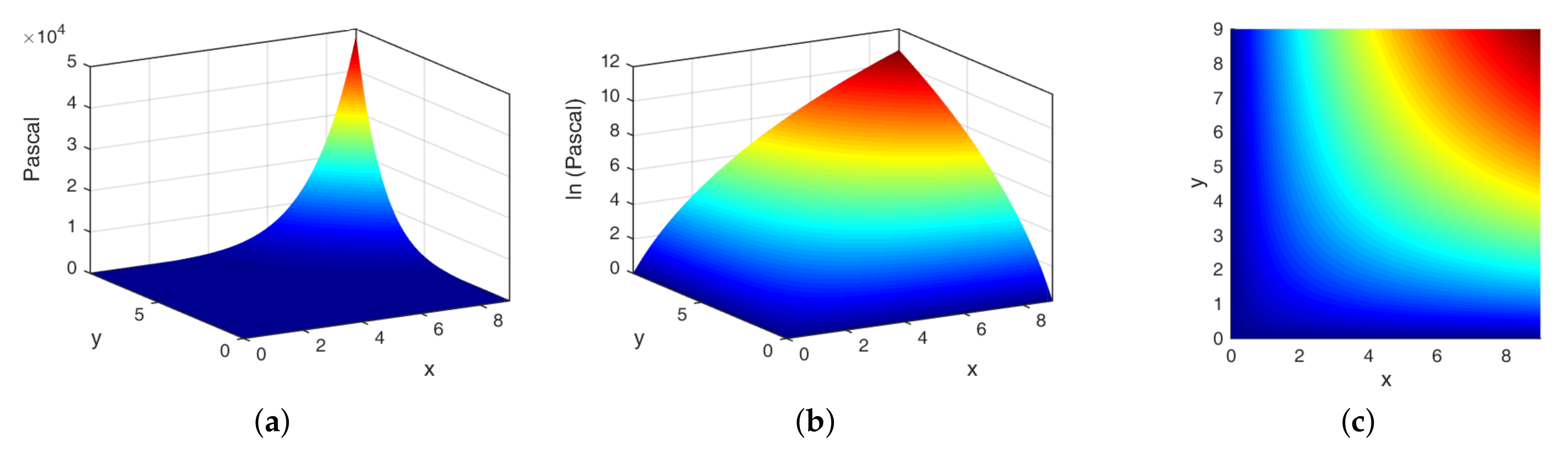
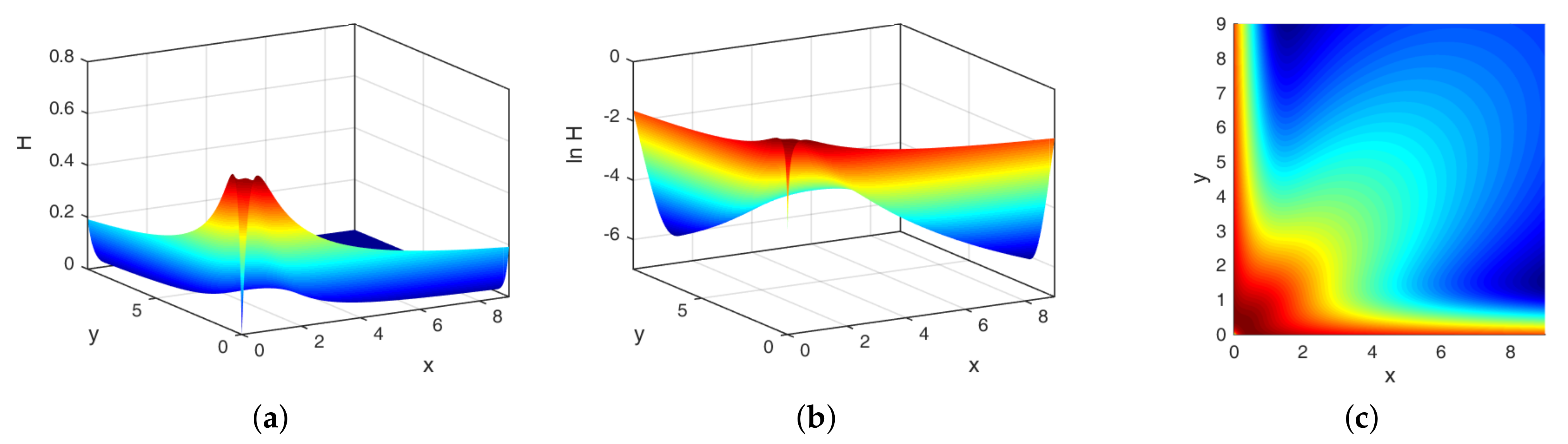
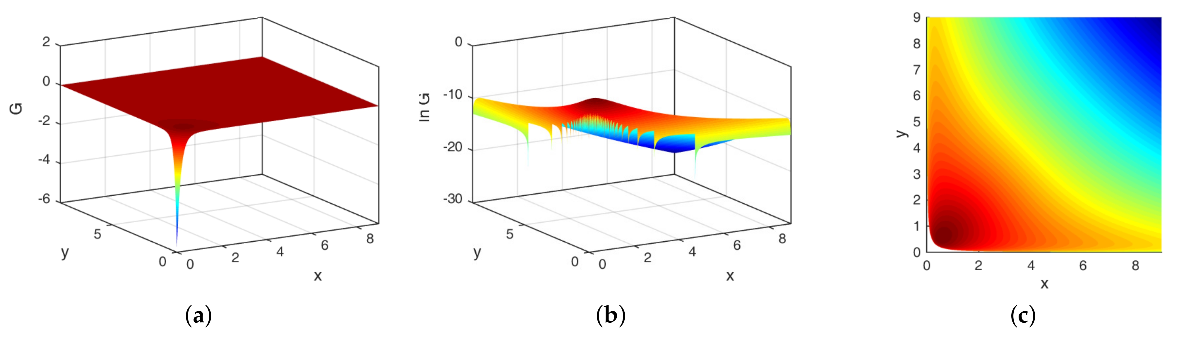
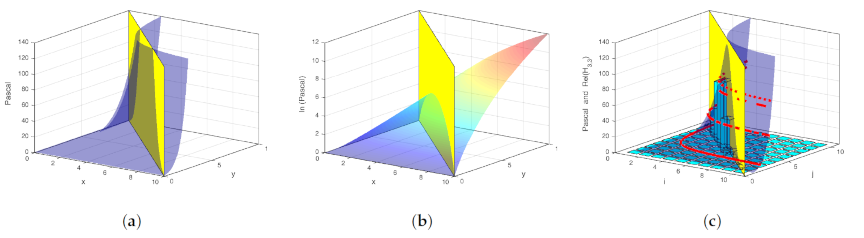
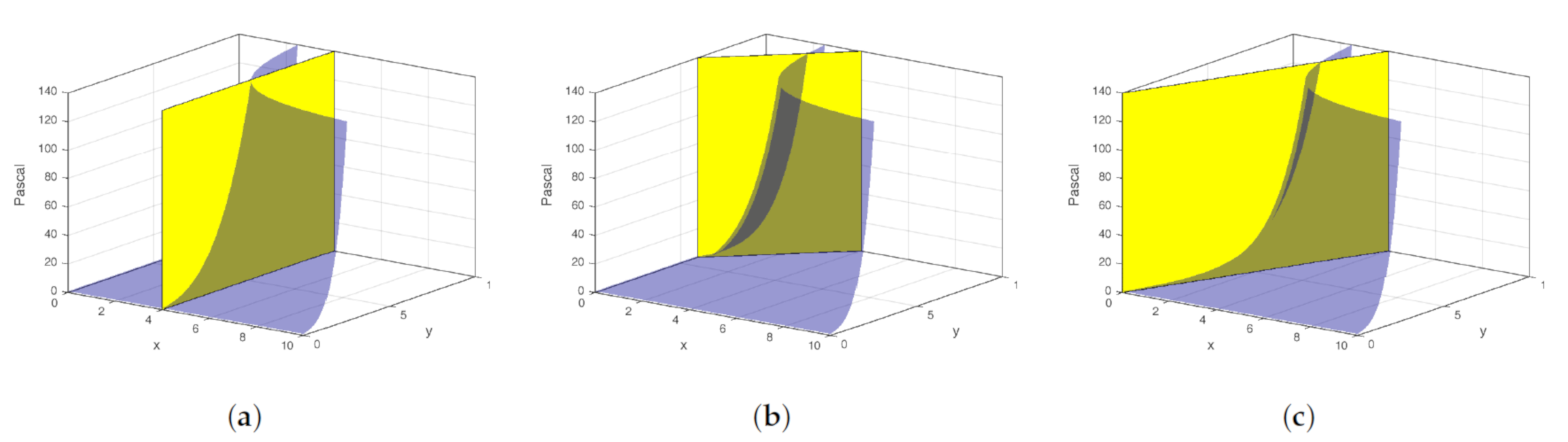
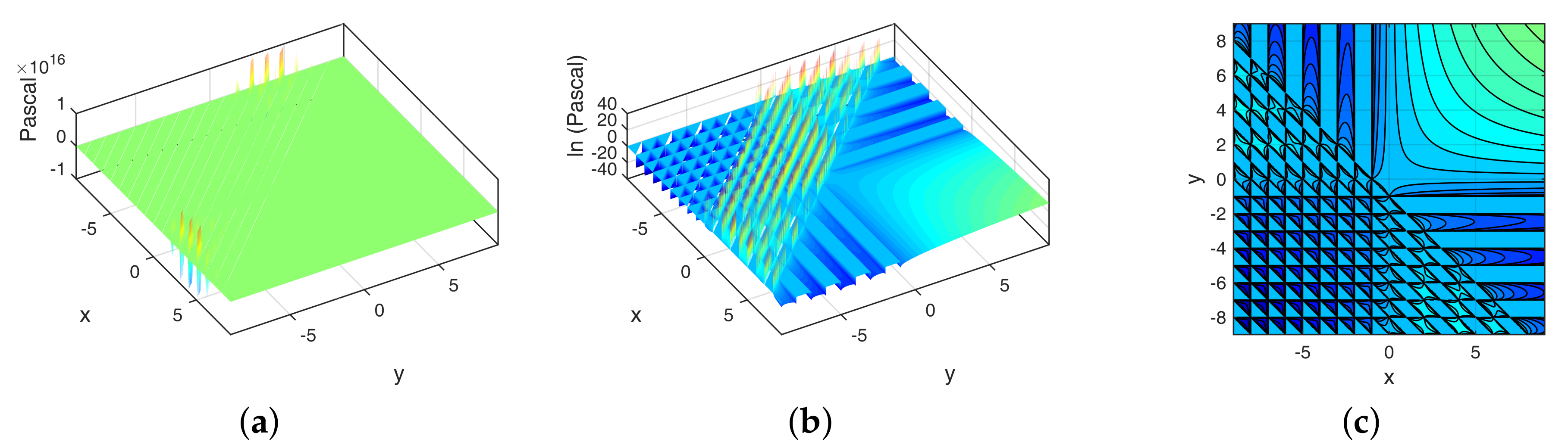
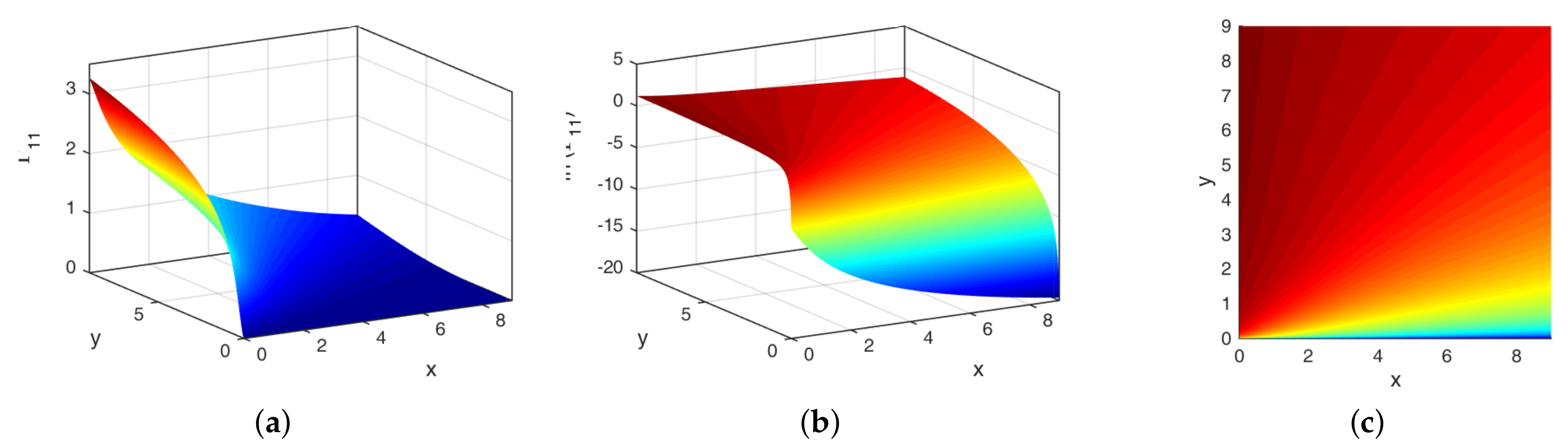
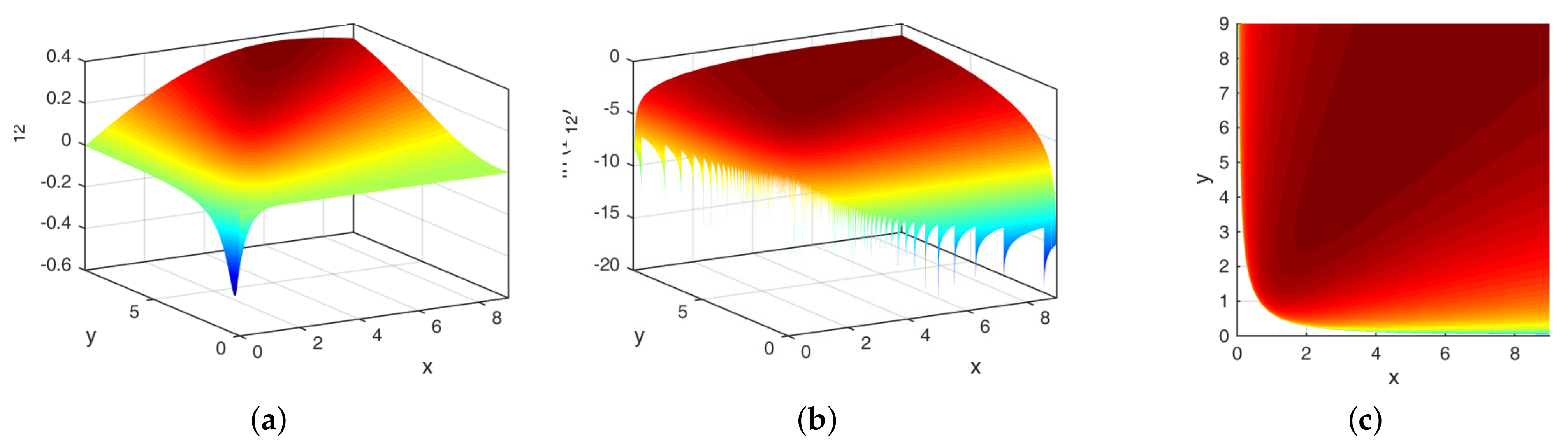
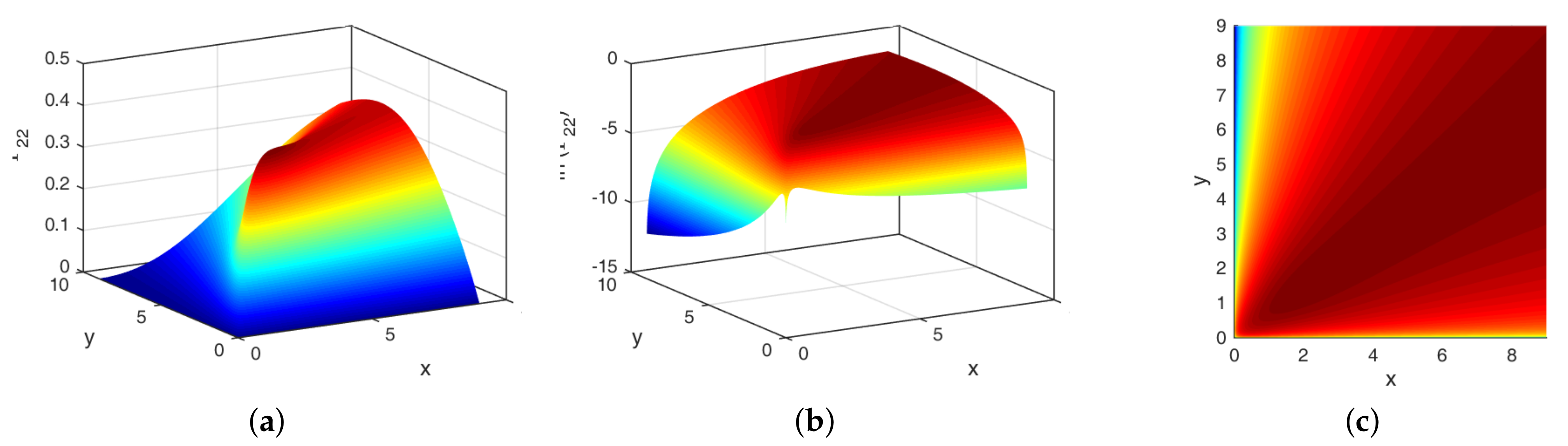
3. A Continuous Pascal’s Surface

Let $xOy$ be a Cartesian coordinate system. Starting from the original Pascal’s triangle depicted in Figure 1a, one should consider the infinite triangle corresponding to $P(\infty )$. Obviously, we can write the numerical entries of this triangle in the lattice points (i.e., points with integer coordinates) from the first quadrant of the Cartesian coordinate system $xOy$. In particular, this maps the components $P{(\infty )}_{ij}$ onto the lattice points $(i,j)$, where $i,j$ are positive integers. Here $i,j$ represent both indices in the matrix $P{(\infty )}_{ij}$ (hence, starting from 1), as well as the integer coordinates $(i,j)=(x+1,y+1)$ in the $xOy$ Cartesian coordinate system. Since $P{(\infty )}_{ij}=\left(\genfrac{}{}{0pt}{}{i+j}{i}\right),$ we may form the triple $\left(i,j,\left(\genfrac{}{}{0pt}{}{i+j}{i}\right)\right)$, which corresponds to a particular point in space. In Figure 1b, we have the graphical representation of the points $\left(i,j,\left(\genfrac{}{}{0pt}{}{i+j}{i}\right)\right)$, where $i,j\in \{1,2,...,10\}.$ To interpolate in between the points $\left(i,j,\left(\genfrac{}{}{0pt}{}{i+j}{i}\right)\right)$, a continuous smooth surface is needed, which can be obtained by simply replacing $\left(\genfrac{}{}{0pt}{}{i+j}{i}\right)$ with its continuous version $\frac{\mathsf{\Gamma }(x+y+1)}{\mathsf{\Gamma }(x+1)\mathsf{\Gamma }(y+1)}$.

Our aim here is to study in the 3-dimensional Euclidean space the surface given by

$$f:{\mathbb{R}}^2\to {\mathbb{E}}^3,f(x,y)=\left(x,y,z(x,y)\right),$$

where

$$z(x,y)=\frac{\mathsf{\Gamma }(x+y+1)}{\mathsf{\Gamma }(x+1)\mathsf{\Gamma }(y+1)},$$

which is a continuous version of $P(\infty )$. This surface is presented in Figure 2 and we shall call it Pascal’s Surface (as in [30]).

We shall use the digamma function $\psi$ which is defined as the logarithmic derivative of the gamma function

$$\psi \left(x\right)=\frac{d}{dx}ln\mathsf{\Gamma }\left(x\right)=\frac{{\mathsf{\Gamma }}^{\prime }\left(x\right)}{\mathsf{\Gamma }\left(x\right)}.$$

For formulas on the geometry of surfaces, we refer the reader to [34].

We have

$$\frac{\partial z}{\partial x}=\frac{1}{\mathsf{\Gamma }(y+1)}\frac{{\mathsf{\Gamma }}^{\prime }(x+y+1)\mathsf{\Gamma }(x+1)-\mathsf{\Gamma }(x+y+1){\mathsf{\Gamma }}^{\prime }(x+1)}{{\mathsf{\Gamma }}^2(x+1)}=$$

$$=\frac{1}{\mathsf{\Gamma }(y+1)}\frac{\psi (x+y+1)\mathsf{\Gamma }(x+y+1)-\mathsf{\Gamma }(x+y+1)\psi (x+1)}{\mathsf{\Gamma }(x+1)}=$$

$$=z(x,y)\left[\psi \right(x+y+1)-\psi (x+1\left)\right],$$

$$\frac{\partial z}{\partial y}=z(x,y)[\psi (x+y+1)-\psi (y+1)].$$

The coefficients of the first fundamental form can be computed as

$$g_{11}=〈\frac{\partial f}{\partial x},\frac{\partial f}{\partial x}〉=1+z^2(x,y){[\psi (x+y+1)-\psi (x+1)]}^2,$$

$$g_{12}=〈\frac{\partial f}{\partial x},\frac{\partial f}{\partial y}〉=z^2(x,y)[\psi (x+y+1)-\psi (x+1)][\psi (x+y+1)-\psi (y+1)],$$

$$g_{22}=〈\frac{\partial f}{\partial y},\frac{\partial f}{\partial y}〉=1+z^2(x,y){[\psi (x+y+1)-\psi (y+1)]}^2.$$

Using these, we determine

$$detg=g_{11}{g}_{22}-g_{12}^2=$$

$$=\{1+z^2(x,y){[\psi (x+y+1)-\psi (x+1)]}^2\}\{(1+z^2(x,y){[\psi (x+y+1)-\psi (y+1)]}^2\}-$$

$$-z^4(x,y){[\psi (x+y+1)-\psi (x+1)]}^2{[\psi (x+y+1)-\psi (y+1)]}^2=$$

$$=1+z^2(x,y){[\psi (x+y+1)-\psi (x+1)]}^2+z^2(x,y){[\psi (x+y+1)-\psi (y+1)]}^2.$$

The unit normal vector $N=\frac{1}{\sqrt{detg}}\frac{\partial f}{\partial x}\times \frac{\partial f}{\partial y}$ to the Pascal’s Surface is given by

$$N=\frac{1}{\sqrt{detg}}(-z(x,y)[\psi (x+y+1)-\psi (x+1)],-z(x,y)[\psi (x+y+1)-\psi (y+1)],1).$$

By straightforward derivations we obtain

$$\frac{{\partial }^{2}z}{\partial x^2}=z(x,y){[\psi (x+y+1)-\psi (x+1)]}^2+z(x,y)[{\psi }^{\prime }(x+y+1)-{\psi }^{\prime }(x+1)],$$

$$\frac{{\partial }^{2}z}{\partial y^2}=z(x,y){[\psi (x+y+1)-\psi (y+1)]}^2+z(x,y)[{\psi }^{\prime }(x+y+1)-{\psi }^{\prime }(y+1)],$$

$$\frac{{\partial }^{2}z}{\partial x\partial y}=z(x,y)[(\psi (x+y+1)-\psi (x+1))(\psi (x+y+1)-\psi (y+1))+{\psi }^{\prime }(x+y+1)].$$

It follows that the coefficients of the second fundamental form are

$$h_{11}=〈\frac{{\partial }^{2}f}{\partial x^2},N〉=\frac{z(x,y)}{\sqrt{detg}}\{{[\psi (x+y+1)-\psi (x+1)]}^2+[{\psi }^{\prime }(x+y+1)-{\psi }^{\prime }(x+1)]\},$$

$$h_{22}=〈\frac{{\partial }^{2}f}{\partial y^2},N〉=\frac{z(x,y)}{\sqrt{detg}}\{{[\psi (x+y+1)-\psi (y+1)]}^2+[{\psi }^{\prime }(x+y+1)-{\psi }^{\prime }(y+1)]\},$$

$$h_{12}=〈\frac{{\partial }^{2}f}{\partial x\partial y},N〉=\frac{z(x,y)}{\sqrt{detg}}[(\psi (x+y+1)-\psi (x+1))(\psi (x+y+1)-\psi (y+1))+{\psi }^{\prime }(x+y+1)].$$

We are now able to compute the mean curvature H and the Gauss curvature G, respectively.

$$H=\frac{g_{22}{h}_{11}-2g_{12}{h}_{12}+g_{11}{h}_{22}}{2detg}=$$

$$=\frac{z(x,y)}{2{(detg)}^{3/2}}\{[1+z^2(x,y){[\psi (x+y+1)-\psi (y+1)]}^2]·$$

$$·\{{[\psi (x+y+1)-\psi (x+1)]}^2+[{\psi }^{\prime }(x+y+1)-{\psi }^{\prime }(x+1)]\}-$$

$$-2z^2(x,y)[\psi (x+y+1)-\psi (x+1)][\psi (x+y+1)-\psi (y+1)]·$$

$$·\{{[\psi (x+y+1)-\psi (y+1)]}^2+[{\psi }^{\prime }(x+y+1)-{\psi }^{\prime }(y+1)]\}+$$

$$+[1+z^2(x,y){[\psi (x+y+1)-\psi (x+1)]}^2]·$$

$$·\{{[\psi (x+y+1)-\psi (y+1)]}^2+[{\psi }^{\prime }(x+y+1)-{\psi }^{\prime }(y+1)]\}.$$

For the Pascal’s Surface from Figure 2, Figure 3a details the mean curvature H. This mean curvature H is also presented in logarithmic scale and as a contour plot in Figure 3b and Figure 3c, respectively.

$$G=\frac{h_{11}{h}_{22}-h_{12}^2}{detg}=$$

$$=\frac{z^2(x,y)}{{det}^{2}g}\{\{{[\psi (x+y+1)-\psi (x+1)]}^2+[{\psi }^{\prime }(x+y+1)-{\psi }^{\prime }(x+1)]\}·$$

$$·\{{[\psi (x+y+1)-\psi (y+1)]}^2+[{\psi }^{\prime }(x+y+1)-{\psi }^{\prime }(y+1)]\}-$$

$$\left.-{[(\psi (x+y+1)-\psi (x+1))(\psi (x+y+1)-\psi (y+1))+{\psi }^{\prime }(x+y+1)]}^2\right\}.$$

Similarly, for the Pascal’s Surface presented in Figure 2, Figure 4a details the Gauss curvature G. This Gauss curvature G is also presented in logarithmic scale and as a contour plot in Figure 4b and Figure 4c, respectively.

In order to establish the differential equations of the geodesics, we first calculate the Christoffel symbols ${\mathsf{\Gamma }}_{ij}^k$, given by

$${\mathsf{\Gamma }}_{ij}^k=\frac{1}{2}\sum _{s=1}^2{g}^{ks}\left(\frac{\partial g_{js}}{\partial x^i}+\frac{\partial g_{is}}{\partial x^j}-\frac{\partial g_{ij}}{\partial x^s}\right),$$

where $x^1=x$, $x^2=y$, and

$$\left(\begin{array}{cc}{g}^{11}& g^{12}\\ g^{12}& g^{22}\end{array}\right)={\left(\begin{array}{cc}{g}_{11}& g_{12}\\ g_{12}& g_{22}\end{array}\right)}^{-1}.$$

We have:

$$\begin{array}{cc}\hfill \frac{\partial g_{11}}{\partial x}& =2z^2(x,y){[\psi (x+y+1)-\psi (x+1)]}^3+\hfill \\ \hfill & +2z^2(x,y)[\psi (x+y+1)-\psi (x+1)][{\psi }^{\prime }(x+y+1)-{\psi }^{\prime }(x+1)]=\hfill \\ \hfill & =2z^2(x,y)[\psi (x+y+1)-\psi (x+1)]·\hfill \\ \hfill & ·[{(\psi (x+y+1)-\psi (x+1))}^2+{\psi }^{\prime }(x+y+1)-{\psi }^{\prime }(x+1)],\hfill \end{array}$$

$$\begin{array}{cc}\hfill \frac{\partial g_{11}}{\partial y}& =2z^2(x,y){[\psi (x+y+1)-\psi (x+1)]}^2[\psi (x+y+1)-\psi (y+1)]+\hfill \\ \hfill & +2z^2(x,y)[\psi (x+y+1)-\psi (x+1)]{\psi }^{\prime }(x+y+1)=\hfill \\ \hfill & =2z^2(x,y)[\psi (x+y+1)-\psi (x+1)]·\hfill \\ \hfill & ·[(\psi (x+y+1)-\psi (x+1))(\psi (x+y+1)-\psi (y+1))+{\psi }^{\prime }(x+y+1)],\hfill \end{array}$$

$$\begin{array}{cc}\hfill \frac{\partial g_{12}}{\partial x}& =2z^2(x,y){[\psi (x+y+1)-\psi (x+1)]}^2[\psi (x+y+1)-\psi (y+1)]+\hfill \\ \hfill & +z^2(x,y)[{\psi }^{\prime }(x+y+1)-{\psi }^{\prime }(x+1)][\psi (x+y+1)-\psi (y+1)]+\hfill \\ \hfill & +z^2(x,y)[\psi (x+y+1)-\psi (x+1)]{\psi }^{\prime }(x+y+1),\hfill \end{array}$$

$$\begin{array}{cc}\hfill \frac{\partial g_{12}}{\partial y}& =2z^2(x,y)[\psi (x+y+1)-\psi (x+1)]{[\psi (x+y+1)-\psi (y+1)]}^2+\hfill \\ \hfill & +z^2(x,y)[\psi (x+y+1)-\psi (x+1)][{\psi }^{\prime }(x+y+1)-{\psi }^{\prime }(y+1)]+\hfill \\ \hfill & +z^2(x,y)[\psi (x+y+1)-\psi (y+1)]{\psi }^{\prime }(x+y+1),\hfill \end{array}$$

$$\begin{array}{cc}\hfill \frac{\partial g_{22}}{\partial x}& =2z^2(x,y)[\psi (x+y+1)-\psi (x+1)]{[\psi (x+y+1)-\psi (y+1)]}^2+\hfill \\ \hfill & +2z^2(x,y)[\psi (x+y+1)-\psi (y+1)]{\psi }^{\prime }(x+y+1)=\hfill \\ \hfill & =2z^2(x,y)[\psi (x+y+1)-\psi (y+1)]·\hfill \\ \hfill & ·[(\psi (x+y+1)-\psi (x+1))(\psi (x+y+1)-\psi (y+1))+{\psi }^{\prime }(x+y+1)],\hfill \end{array}$$

$$\begin{array}{cc}\hfill \frac{\partial g_{22}}{\partial y}& =2z^2(x,y){[\psi (x+y+1)-\psi (y+1)]}^3+\hfill \\ \hfill & +2z^2(x,y)[\psi (x+y+1)-\psi (y+1)][{\psi }^{\prime }(x+y+1)-{\psi }^{\prime }(y+1)]=\hfill \\ \hfill & =2z^2(x,y)[\psi (x+y+1)-\psi (y+1)]·\hfill \\ \hfill & ·[{(\psi (x+y+1)-\psi (y+1))}^2+{\psi }^{\prime }(x+y+1)-{\psi }^{\prime }(y+1)].\hfill \end{array}$$

The Christoffel symbols can be written as:

$$\begin{array}{cc}\hfill {\mathsf{\Gamma }}_{11}^1& =\frac{1}{2}\left[g^{11}\frac{\partial g_{11}}{\partial x}+g^{12}\left(2\frac{\partial g_{12}}{\partial x}-\frac{\partial g_{11}}{\partial y}\right)\right]=\hfill \\ \hfill & =\frac{z^2(x,y)}{detg}\{[1+z^2(x,y){[\psi (x+y+1)-\psi (y+1)]}^2][\psi (x+y+1)-\psi (x+1)]·\hfill \\ \hfill & ·[{(\psi (x+y+1)-\psi (x+1))}^2+{\psi }^{\prime }(x+y+1)-{\psi }^{\prime }(x+1)]-\hfill \\ \hfill & -z^2(x,y)[\psi (x+y+1)-\psi (x+1)][\psi (x+y+1)-\psi (y+1)]·\hfill \\ \hfill & ·\left\{2{[\psi (x+y+1)-\psi (x+1)]}^2[\psi (x+y+1)-\psi (y+1)]+\right.\hfill \\ \hfill & +[{\psi }^{\prime }(x+y+1)-{\psi }^{\prime }(x+1)][\psi (x+y+1)-\psi (y+1)]+\hfill \\ \hfill & +[\psi (x+y+1)-\psi (x+1)]{\psi }^{\prime }(x+y+1)-[\psi (x+y+1)-\psi (x+1)]·\hfill \\ \hfill & \left.·[(\psi (x+y+1)-\psi (x+1))(\psi (x+y+1)-\psi (y+1))+{\psi }^{\prime }(x+y+1)]\right\}\},\hfill \end{array}$$

$$\begin{array}{cc}\hfill {\mathsf{\Gamma }}_{12}^1& =\frac{1}{2}\left(g^{11}\frac{\partial g_{11}}{\partial y}+g^{12}\frac{\partial g_{22}}{\partial x}\right)=\hfill \\ \hfill & =\frac{z^2(x,y)}{detg}\{[1+z^2(x,y){[\psi (x+y+1)-\psi (y+1)]}^2][\psi (x+y+1)-\psi (x+1)]·\hfill \\ \hfill & ·[(\psi (x+y+1)-\psi (x+1))(\psi (x+y+1)-\psi (y+1))+{\psi }^{\prime }(x+y+1)]-\hfill \\ \hfill & -\left[\psi \right(x+y+1)-\psi (x+1\left)\right]\left[\psi \right(x+y+1)-\psi (y+1\left)\right]\left[\psi \right(x+y+1)-\psi (y+1\left)\right]·\hfill \\ \hfill & ·[(\psi (x+y+1)-\psi (y+1))(\psi (x+y+1)-\psi (x+1))+{\psi }^{\prime }(x+y+1)]\},\hfill \end{array}$$

$$\begin{array}{cc}\hfill {\mathsf{\Gamma }}_{22}^1& =\frac{1}{2}\left[g^{11}\left(2\frac{\partial g_{12}}{\partial y}-\frac{\partial g_{22}}{\partial x}\right)+g^{12}\frac{\partial g_{22}}{\partial y}\right]=\hfill \\ \hfill & =\frac{z^2(x,y)}{detg}\{[1+z^2(x,y){[\psi (x+y+1)-\psi (y+1)]}^2]·\hfill \\ \hfill & ·\left\{2{[\psi (x+y+1)-\psi (y+1)]}^2[\psi (x+y+1)-\psi (x+1)]+\right.\hfill \\ \hfill & +[{\psi }^{\prime }(x+y+1)-{\psi }^{\prime }(y+1)][\psi (x+y+1)-\psi (x+1)]+\hfill \\ \hfill & +[\psi (x+y+1)-\psi (y+1)]{\psi }^{\prime }(x+y+1)-[\psi (x+y+1)-\psi (y+1)]·\hfill \\ \hfill & ·[(\psi (x+y+1)-\psi (y+1))(\psi (x+y+1)-\psi (x+1))+{\psi }^{\prime }(x+y+1)]-\hfill \\ \hfill & -\left[\psi \right(x+y+1)-\psi (x+1\left)\right]\left[\psi \right(x+y+1)-\psi (y+1\left)\right]·\hfill \\ \hfill & ·[{(\psi (x+y+1)-\psi (y+1))}^2+{\psi }^{\prime }(x+y+1)-{\psi }^{\prime }(y+1)]\left\}\right\}.\hfill \end{array}$$

Appendix A presents the graphical representations of these Christoffel symbols computed for the Pascal’s Surface.

The equations of the geodesics are

$$\left\{\begin{array}{c}\frac{d^{2}x}{d{t}^2}+{\mathsf{\Gamma }}_{11}^1{\left(\frac{dx}{dt}\right)}^2+2{\mathsf{\Gamma }}_{12}^1\frac{dx}{dt}\frac{dy}{dt}+{\mathsf{\Gamma }}_{22}^1{\left(\frac{dy}{dt}\right)}^2=0,\hfill \\ \frac{d^{2}y}{d{t}^2}+{\mathsf{\Gamma }}_{11}^2{\left(\frac{dx}{dt}\right)}^2+2{\mathsf{\Gamma }}_{12}^2\frac{dx}{dt}\frac{dy}{dt}+{\mathsf{\Gamma }}_{22}^2{\left(\frac{dy}{dt}\right)}^2=0.\hfill \end{array}\right.$$

By substituting ${\mathsf{\Gamma }}_{11}^1,{\mathsf{\Gamma }}_{12}^1$ and ${\mathsf{\Gamma }}_{22}^1$ computed above, we can write the first equation. Interchanging x and y, we obtain the second equation.

4. Discussions and Conclusions

The results we have presented here are normal continuations of those reported in [26,30]. On the one side, our results are limited to positive real numbers, but they are thoroughly detailed with respect to geometric proprieties associated to Pascal’s Surface, properties which have never been analyzed before. Obviously, this line of research can and should be continued.

On the other side, let us see how such theoretical results are to be linked to more practical applications, such as the reliability polynomials. We shall take as a particular example the following reliability polynomial expressed in Bernstein form $Rel(H_{3,3},p)=\mathbf{8}{p}^3{q}^6+\mathbf{42}{p}^4{q}^5+\mathbf{84}{p}^5{q}^4+\mathbf{76}{p}^6{q}^3+36p^7{q}^2+9p^{8}q+p^9$, where $q=1-p$. This is the reliability polynomial associated with $H_{3,3}$, which is a classical hammock network having $w=l=3$ (w is the width and l is the length of the network); for details see [5,12]. A reliability polynomial will always have the first l coefficients 0, while the last w coefficients are all identical to the corresponding binomial coefficients. Thus, the coefficients of interest are the remaining $lw-l-w$ ones (the four red coefficients of $Rel(H_{3,3},p)$, namely: 8, 42, 84, and 76). The level curves corresponding to these four coefficients of interest can be seen in Figure 5c (also in red).

One additional remark is that computations such as the ones performed for generating these images are highly demanding and an option we intend to pursue is to rely on approximations which, while not absolutely accurate, would allow us to significantly reduce the computing time (time-complexity). These could also move us forward on time-efficient approximations of the coefficients of reliability polynomials, a topic of high interest in the context of advanced nanoscale CMOS transistors fabricated using EUV lithography [35].

Obviously, the surface we have investigated here was limited to the positive quadrant because all the coefficients of a Bernstein polynomial are positive. In particular, for reliability polynomials all the coefficients are integers (resulting from counting processes, i.e., particular numbers of paths), and one more variable is an integer as well (representing an index/exponent). This means that a normal continuation would be to investigate particular cuts on this surface, i.e., not only horizontal cuts which generate level curves. That is why we plan to investigate the intersection of Pascal’s Surface with at least three type of vertical cuts: (i) parallel with either $Ox$ or $Oy$; (ii) parallel with the line bisecting the first and third quadrants; and finally, (iii) radial ones from the origin (see Figure 6).

On the other hand, the approach we have presented here is generic, and the associated Pascal’s Surface for a small range of real values can be seen in Figure 7. This reveals (very) complex surfaces on the other three quadrants, which might be of interest in the longer run.

Last but not least, we expect that relying on a fractional view might allow us to study other curves on Pascal’s Surface. One of us has already been working on a related subject by defining the notions of equiaffine arclength and curvature with fractional order [36], a paper which has introduced a classification of the plane curves of constant equiaffine curvature with fractional order, while also providing several explanatory examples. That is why we plan to continue exploring symmetries appearing on such surfaces.

References

1. Beiu, V. A novel highly reliable low-power nano architecture—When von Neumann augments Kolmogorov. In Proceedings of the 15th IEEE International Conference on Application-Specific Systems, Architectures and Processors (ASAP’04), Galveston, TX, USA, 27–29 September 2004; IEEE: Piscataway, NJ, USA; pp. 167–177. [Google Scholar] [CrossRef]
2. Roy, S.; Beiu, V. Majority multiplexing—Economical redundant fault-tolerant design for nano architectures. IEEE Trans. Nano. 2005, 4, 441–451. [Google Scholar] [CrossRef]
3. Beiu, V.; Ibrahim, W. Devices and input vectors are shaping von Neumann multiplexing. IEEE Trans. Nano. 2011, 10, 606–616. [Google Scholar] [CrossRef]
4. von Neumann, J. Probabilistic logics and the synthesis of reliable organisms from unreliable components. In Automata Studies (AM-34); Shannon, C.E., McCarthy, J., Eds.; Princeton Univ. Press: Princeton, NJ, USA, 1956; pp. 43–98. Available online: https://archive.org/details/vonNeumann_Prob_Logics_Rel_Org_Unrel_Comp_Caltech_1952/mode/2up (accessed on 6 February 2022). [CrossRef] [Green Version]
5. Moore, E.F.; Shannon, C.E. Reliable circuits using less reliable relays—Part I. J. Frankl. Inst. 1956, 262, 191–208. [Google Scholar] [CrossRef]
6. Moore, E.F.; Shannon, C.E. Reliable circuits using less reliable relays—Part II. J. Frankl. Inst. 1956, 262, 281–297. [Google Scholar] [CrossRef]
7. International Roadmap for Devices and Systems (IRDS™), 2021 Edition; IEEE: Piscataway, NJ, USA. Available online: https://irds.ieee.org/editions/2021 (accessed on 6 February 2022).
8. Dixit, H.D.; Pendharkar, S.; Beadon, M.; Mason, C.; Chakravarthy, T.; Muthiah, B.; Sankar, S. Silent data corruptions at scale. Tech. Rep. 2021, arXiv:2102.11245. Available online: https://arxiv.org/abs/2102.11245 (accessed on 6 February 2022).
9. Hochschild, P.H.; Turner, P.; Mogul, J.C.; Govindaraju, R.; Ranganathan, P.; Culler, D.E.; Vahdat, A.M. Cores that don’t count. In Proceedings of the Workshop Hot Topics in Operating Systems (HotOS’21), Ann Arbor, MI, USA, 1–3 June 2021; ACM Press: New York, NY, USA, 2021; pp. 9–16. [Google Scholar] [CrossRef]
10. Dăuş, L.; Beiu, V. Lower and upper reliability bounds for consecutive-k-out-of-n:F systems. IEEE Trans. Rel. 2015, 64, 1128–1135. [Google Scholar] [CrossRef]
11. Beiu, V.; Dăuş, L. Reliability bounds for two dimensional consecutive systems. Nano Comm. Netw. 2015, 6, 145–152. [Google Scholar] [CrossRef]
12. Cowell, S.R.; Beiu, V.; Dăuş, L.; Poulin, P. On the exact reliability enhancements of small hammock networks. IEEE Access 2018, 6, 25411–25426. [Google Scholar] [CrossRef]
13. Beiu, V.; Drăgoi, V.-F.; Beiu, R.-M. Why reliability for computing needs rethinking. In Proceedings of the Conference Rebooting Computing (ICRC 2020), Atlanta, GA, USA, 1–3 December 2020; IEEE: Piscataway, NJ, USA, 2020; pp. 16–25. [Google Scholar] [CrossRef]
14. Bernstein, S.N. Démonstration du théorème de Weierstrass fondée sur le calcul des probabilities [Proof of the theorem of Weierstrass based on the calculus of probabilities]. Comm. Kharkov Math. Soc. 1912, 13, 1–2. [Google Scholar]
15. Colbourn, C.J. The Combinatorics of Network Reliability; Oxford University Press: New York, NY, USA, 1987. [Google Scholar]
16. Chari, M.; Colbourn, C.J. Reliability polynomials: A survey. J. Comb. Inf. Syst. Sci. 1997, 22, 177–193. [Google Scholar]
17. Drăgoi, V.-F.; Beiu, V. Fast reliability ranking of matchstick minimal networks. Networks 2021, 1–22, Early view. [Google Scholar] [CrossRef]
18. Pérez-Rosés, H. Sixty years of network reliability. Maths. Comp. Sci. 2018, 12, 275–293. [Google Scholar] [CrossRef]
19. Brown, J.I.; Colbourn, C.J.; Cox, D.; Graves, C.; Mol, L. Network reliability: Heading out on the highway. Networks (Sp. Iss. Celebr. 50 Years Networks) 2021, 77, 146–160. [Google Scholar] [CrossRef]
20. Pascal, B. Traité du Triangle Arithmétique, Avec Quelques Autres Petit Traitez sur la Mesme Matiere; G. Desprez: Paris, France, 1665; Available online: https://gallica.bnf.fr/ark:/12148/btv1b86262012/f1.image (accessed on 6 February 2022).
21. Bondarenko, B.A. Generalized Pascal Triangles and Pyramids—Their Fractals, Graphs, and Applications. Izdatel’stvo “FAN” RUz: Tashkent, 1990 [Translated by R.C. Bollinger, 1993]. Available online: https://www.fq.math.ca/pascal.html (accessed on 6 February 2022).
22. Gross, J.L. Combinatorial Methods with Computer Applications; Chapman and Hall/CRC, Taylor & Francis Group: London, UK, 2007; Available online: http://www.cs.columbia.edu/~cs4205/files/CM4.pdf (accessed on 6 February 2022).
23. Lawrencenko, S.A.; Magomedov, A.M.; Zgonnik, L.V. Problems with parameters and binomial identities. Math. Sch. 2018, 6, 16–26. (In Russian) [Google Scholar]
24. Cobeli, C.; Zaharescu, A. Promenade around Pascal triangle—Number motives. Bull. Math. Soc. Sci. Math. Roumanie 2013, 56, 73–98. [Google Scholar]
25. Raab, J.A. A generalization of the connection between the Fibonacci sequence and Pascal’s triangle. Fibonacci Q. 1963, 1, 21–31. [Google Scholar]
26. Fowler, D. The binomial coefficient function. Amer. Math. Month. 1996, 103, 1–17. [Google Scholar] [CrossRef]
27. Fowler, D. A simple approach to the factorial function. Math. Gazette 1996, 80, 378–381. [Google Scholar] [CrossRef]
28. Fowler, D. A simple approach to the factorial function—The next step. Math. Gazette 1999, 83, 53–57. [Google Scholar] [CrossRef]
29. Lampret, V. Estimating the sequence of real binomial coefficients. J. Inequal. Pure Appl. Math. 2006, 7, art. 166. [Google Scholar]
30. Pellicer, R.; Alvo, A. Modified Pascal Triangle and Pascal Surfaces. Tech. Rep. academia.edu:956605. 2012. Available online: http://www.academia.edu/956605 (accessed on 6 February 2022).
31. Salwinski, D. The continuous binomial coefficient: An elementary approach. Amer. Math. Mon. 2018, 125, 231–244. [Google Scholar] [CrossRef]
32. Formichella, S.; Straub, A. Gaussian binomial coefficients with negative arguments. Ann. Comb. 2019, 23, 725–748. [Google Scholar] [CrossRef] [Green Version]
33. Smith, S.T. The binomial coefficient C(n,x) for arbitrary x. Online J. Anal. Comb. 2020, 15, 176. [Google Scholar]
34. do Carmo, M. Differential Geometry of Curves and Surfaces; Prentice-Hall: Englewood Cliffs, NJ, USA, 1976. [Google Scholar]
35. Beiu, V. The unfolding road from dust to trust. In Proceedings of the International Conference Advances in 3OM (Adv3OM 2021), Timisoara, Romania, 13–16 December 2021; SPIE: Bellingham, WA, USA, 2021. in press. [Google Scholar]
36. Aydin, M.E.; Mihai, A.; Yokus, A. Applications of fractional calculus in equiaffine geometry: Plane curves with fractional order. Math. Methods Appl. Sci. 2021, 44, 13659. [Google Scholar] [CrossRef]
Figure 1. Classical (discrete) Pascal’s triangle: (a) Original Blaise Pascal’s writing, (b) 3D bar graph of P ( ) , and (c) 3D bar graph of ln P ( ) .
Symmetry 14 00411 g001
Figure 2. Surface matching the classical (discrete) Pascal’s triangle (presented in Figure 1): (a) Surface (linear scale), (b) Surface (logarithmic scale), and (c) Contours (Figure 2b).
Symmetry 14 00411 g002
Figure 3. The mean curvature H (of the surface presented in Figure 2): (a) Mean curvature H (linear scale), (b) Mean curvature H (logarithmic scale), and (c) Contours of H (Figure 3b).
Symmetry 14 00411 g003
Figure 4. The Gauss curvature G (of the surface presented in Figure 2): (a) Gauss curvature G (linear scale), (b) Gauss curvature G (logarithmic scale), and (c) Contours of G (Figure 4b).
Symmetry 14 00411 g004
Figure 5. Example for the continuous Pascal’s Surface: (a) Surface matching Figure 1b (P), (b) Surface matching Figure 1c ( ln P ), and (c) Surface, H 3 , 3 (bars), and level curves.
Symmetry 14 00411 g005
Figure 6. Three different cuts on Pascal’s Surface: (a) Parallel with O y , (b) Parallel with one of the bisecting lines, and (c) Radial from the origin.
Symmetry 14 00411 g006
Figure 7. Pascal’s Surface for 10 < x , y < 10 : (a) Linear view (large oscillations), (b) Logarithmic view, and (c) Contours of Figure 7b.
Symmetry 14 00411 g007
Publisher’s Note: MDPI stays neutral with regard to jurisdictional claims in published maps and institutional affiliations.