Similarity Measures Based on T-Spherical Fuzzy Information with Applications to Pattern Recognition and Decision Making

Abstract

T-spherical fuzzy set (TSFS) is a fuzzy layout aiming to provide a larger room for the processing of uncertain information-based data where four aspects of unpredictable information are studied. The frame of picture fuzzy sets (PFSs) and intuitionistic fuzzy sets (IFSs) provide limited room for processing such kinds of information. On a scale of zero to one, similarity measures (SMs) are a tool for evaluating the degrees of resemblance between various items or phenomena. The goal of this paper is to investigate the shortcomings of picture fuzzy (PF) SMs in order to introduce a new SM in a T-spherical fuzzy (TSF) environment. The newly improved SM has a larger ground for accommodating the uncertain information with three degrees and is also responsible for the reduction of information loss. The proposed SM’s validity is demonstrated mathematically and by examples. To examine the application of the suggested SM two real-life issues are discussed, including the concerns of medical diagnosis and pattern recognition. A comparison of the suggested SMs with current SMs is also made to assess the proposed work’s reliability. Since symmetric triangular fuzzy numbers are quite useful in database acquisition, we will consider the proposed SM for symmetric T-spherical triangular fuzzy numbers in the near future.

1. Introduction

Zadeh [1] conceived the concept of fuzzy sets (FSs) in 1965. In FSs, a function of memberships on a scale of $\left\{0,1\right\}$ was used to show the degree of membership (DM) of an element in a set with the degree of non-membership (DNM) calculated by subtracting DM from 1, i.e., $DNM=1-DM$. Later, Atanassov [2] refined the concept from FSs to intuitionistic fuzzy sets (IFSs) which define DM and DNM separately, but have their full scope in the range of $\left\{0, 1\right\}$, i.e., $DM+DNM\in \left[0, 1\right].$ Atanassov’s model of IFSs also has significant limitations, as the sum of DM and DNM might sometimes surpass the range of $\left\{0, 1\right\}$. As a result, Yager [3] developed Pythagorean FSs (PyFSs) by expanding the space of IFSs with a flexible constraint, i.e., $D{M}^2+DN{M}^2\in \left[0, 1\right]$. Yager [4] also introduced the concept of q-Rung Orthopair FSs (q-ROFSs). In q-ROFSs, the sum of qth power of DM and qth power of DNM is equal to or less than 1, i.e., $D{M}^q+DN{M}^q\in \left[0, 1\right]$.

Although Atanassov’s IFSs model revealed Zadeh’s notion of FSs, there exist some scenarios where there are more than two options including the degree of abstinence (DA) and degree of refusal (DR). In this case, IFSs failed to comment on these uncertainties. By considering all these shortcomings of IFSs, Cuong [5] devised picture FSs (PFSs) which have three membership functions represented by DM, DA, and DNM with a restriction that their total should lie in the range of $\left\{0, 1\right\}$, i.e., $DM+DA+DNM\in \left[0, 1\right].$ The term $\left(1-\left(DM+DA+DNM\right)\right)$ was referred to as the DR of an element of a PFS. Some recent studies on PFSs can be found in [6,7]. PFSs broadened the scope of FSs and IFSs, but there are still constraints, and we cannot assign DM, DA, and DNM independently. Mahmood et al. [8] proposed the idea of spherical fuzzy sets (SFSs) as a modification of PFSs by enhancing the range of PFSs by realizing the structures of FSs, IFSs, and PFSs. Similarly, the sum of DM, DA, and DNM may be more than the unit interval in the structure of SFSs, and their squares must fall within the unit interval which is defined as $D{M}^2+D{A}^2+DN{M}^2\in \left[0, 1\right]$. SFSs have a wider range than PFSs due to their new restriction. However, even squaring is not enough as the squared sum of DM, DA, and DNM exceeds the unit interval, i.e.,$D{M}^2+D{A}^2+DN{M}^2>1$. To deal with this kind of situation, Mahmood et al. [8] also presented a modification of SFSs which was known as T-spherical FSs (TSFSs). TSFSs have the condition that $D{M}^n+D{A}^n+DN{M}^n\in \left[0, 1\right]$ where $\mathrm{n}\in {\mathbb{Z}}^{+}$. We see that TSFSs are a more generic version of IFSs, PFSs, and SFSs. Some recent work on SFSs and TSFSs can be found in [9,10,11].

Similarity measures (SMs) are used to assess the degree of similarity between different items or phenomena on a scale of zero to one. SMs had been discussed on FSs since Zadeh [1] introduced FSs. For example, Chen et al. [12] proposed the comparison of SMs of fuzzy values in which they use fuzzy values to compare the attributes of several SMs. Yang et al. [13] considered similarity measures between fuzzy numbers and then applied them to database acquisition. Since Atanassov [2] proposed IFSs as a generalization of FSs, despite the introduction of many SMs for FSs, they were unable to solve problems when placed in an IFS environment. As a result, Dengfeng and Chuntian [14] proposed new SMs on IFSs that can cope with the problems given in the environment of IFSs. Liang and Shi [15] presented a new SM on IFSs based on the fact that the previously defined SMs are not useful in some situations. Li et al. [16] evaluated and summarized known SMs between IFSs and intuitionistic vague sets (IVSs). The benefits of each SM are explored as well as the circumstances in which they may or may not operate as intended. For IFSs induced by the Jaccard index, Hwang et al. [17] developed a novel SM. They demonstrate that the recommended SMs are more logical than the alternatives using numerical examples. By expanding the space of IFSs with a flexible constraint, Yager [3] established PyFSs. To cope with the data given in the PyFSs environment, SMs for PyFSs were also introduced. Wei and Wei [18] presented 10 SMs between PyFSs based on the cosine function with applications to medical diagnosis. Zeng et al. [19] proposed distance and SMs of PyFSs and used them in multiple criteria group decision making. Peng and Garg [20] proposed multiparametric SMs between PyFSs and they were put to the test by applying them to pattern recognition problems. Based on the Hausdorff metric, Hussain and Yang [21] presented distances and SMs of PyFSs and then gave a fuzzy TOPSIS. Concerning SMs for q-ROFSs, PFSs, and SFSs, Wang et al. [22] gave the SMs of q-ROFSs based on cosine functions.

Wei [23] considered SMs for PFSs and then used them to recognize construction materials and mineral fields. SMs for SFS based cosine function were proposed by Mahmood et al. [24] with applications in pattern recognition and medical diagnosis. Rafiq et al. [25] proposed the cosine SM of SFSs and offered a number of numerical decision-making applications to test the proposed SM’s correctness. After Mahmood et al. [8] presented the concept of TSFSs, which is the extension of FSs, IFSs, PFSs, and SFSs, Ullah et al. [26] proposed SMs for TSFSs with pattern recognition applications. Ye [27] proposed SMs based on the modified distance of neutrosophic Z-number sets and a multi-attribute decision-making technique. For pattern recognition and medical diagnostics, Mahmood et al. [28] suggested hybrid vector similarity metrics based on complex hesitant fuzzy sets. Power aggregation techniques and SMs based on improved intuitionistic hesitant fuzzy sets were suggested by Mahmood et al. [29], as well as their applicability to multiple attribute decision making. Chinram et al. [30] suggested and used a series of novel cosine SMs based on hesitant complex fuzzy sets. Mahmood et al. [31] introduced Jaccard and dice SMs and their applications based on complicated dual hesitant fuzzy sets that are one-of-a-kind.

Although Ullah et al. [26] had proposed SMs for TSFSs, we shall establish a new SM for TSFSs in this paper so that it can be a generalized form of PFSs as done in the previously proposed SMs by Luo and Zhang [32]. We begin by reviewing previously defined SMs for PFSs and observe their limitations when it comes to their applicability. The main reason to develop a new SM was the fact that TSFSs provide a flexible and larger range for data representation under uncertain circumstances. To check the effectiveness of the proposed SMs we provide an example of a pattern recognition system with its application for decision-making. It can also be determined which example is more suitable and effective by having a comparative study of both examples with the previously defined SMs. The followings are the major contributions of this paper:

• To view/observe the limitations of the previous SMs because of their applicability.
• To propose a new SM with flexibility in the environment of TSFSs.
• To check the validity of the proposed SM using some results.
• To apply the proposed SM in pattern recognition and decision making.
• To compare the proposed work with previous works by a comparative analysis where the efficacy of the suggested SM is discussed.

The rest of the paper is organized as follows. In Section 2, we go over some key TSFS concepts. A new SM for TSFSs is proposed in Section 3. In Section 4, the suggested SM is used to recognize patterns in a pattern recognition system as well as to make decisions. In Section 5, we come to a conclusion.

2. Preliminaries

Some SFSs and TSFSs definitions are outlined in this section. Throughout the work, $\mathrm{X}$ denotes a universal set.

Definition 1

[8]. A SFS $\mathrm{S}$ on $\mathrm{X}$ is written as:

$$\mathrm{S}=\left\{\mathsf{\mu }\left(\mathsf{ҳ}\right), \mathsf{\eta }\left(\mathsf{ҳ}\right), \mathrm{v}\left(\mathsf{ҳ}\right):0\le {\mathsf{\mu }}^2\left(\mathsf{ҳ}\right)+{\mathsf{\eta }}^2\left(\mathsf{ҳ}\right)+{\mathrm{v}}^2\left(\mathsf{ҳ}\right)\le 1\right\}$$

such that $\mathsf{\mu }$, $\mathsf{\eta },$and $\mathrm{v}$ranging from $0$to $1$denote the DM, DA, and DNM of $\mathsf{ҳ}\in \mathrm{X},$respectively, and $\mathrm{r}\left(\mathsf{ҳ}\right)=\sqrt{1-\mathrm{sum}\left({\mathsf{\mu }}^2,{\mathsf{\eta }}^2,{ \mathrm{v}}^2\right)},$with $\mathrm{sum}\left({\mathsf{\mu }}^2,{\mathsf{\eta }}^2,{ \mathrm{v}}^2\right)={\mathsf{\mu }}^2+{\mathsf{\eta }}^2+{ \mathrm{v}}^2,$is the DR of $\mathsf{ҳ}$in $\mathrm{S},$where$\left(\mathsf{\mu }, \mathsf{\eta }, \mathrm{v}\right)$is considered as a spherical fuzzy number (SFN) for $\mathrm{S}$.

Definition 2

[8]. A TSFS$\mathrm{S}$  $on \mathrm{X}$ is written as:

$$\mathrm{S}=\left\{\mathsf{\mu }\left(\mathsf{ҳ}\right), \mathsf{\eta }\left(\mathsf{ҳ}\right), \mathrm{v}\left(\mathsf{ҳ}\right):0\le {\mathsf{\mu }}^{\mathrm{n}}\left(\mathsf{ҳ}\right)+{\mathsf{\eta }}^{\mathrm{n}}\left(\mathsf{ҳ}\right)+{\mathrm{v}}^{\mathrm{n}}\left(\mathsf{ҳ}\right)\le 1\right\}$$

such that $\mathsf{\mu }$, $\mathsf{\eta },$and $\mathrm{v}$ranging from $0$to $1$denote the DM, DA, and DNM of $\mathsf{ҳ}\in \mathrm{X},$respectively, for $\mathrm{n}\in {\mathbb{Z}}^{+},$and $\mathrm{r}\left(\mathsf{ҳ}\right)=\sqrt[\mathrm{n}]{1-\mathrm{sum}\left({\mathsf{\mu }}^{\mathrm{n}},{\mathsf{\eta }}^{\mathrm{n}},{ \mathrm{v}}^{\mathrm{n}}\right)}$is the DR of $\mathsf{ҳ}$in $\mathrm{S}$. $\left(\mathsf{\mu }, \mathsf{\eta }, \mathrm{v}\right)$is considered as a T-spherical fuzzy number (TSFN).

Now, some notions of SMs are comparatively examined. The definitions described in this section provided a base for this work.

Definition 3

[2]. For two IFNs $\mathsf{Á}=\left({\mathsf{\mu }}_{\mathsf{Á}},{ \mathrm{v}}_{\mathsf{Á}}\right)$ and $\mathrm{B}=\left({\mathsf{\mu }}_{\mathrm{B}},{ \mathrm{v}}_{\mathrm{B}}\right)$, an SM is written as:

$$Ś\left(\mathsf{Á}, \mathrm{B}\right)=\frac{1}{\mathrm{m}}{\displaystyle \sum }_{ї=1}^{\mathrm{m}}\frac{{\mathsf{\mu }}_{{\mathsf{Á}}_{{\mathsf{ҳ}}_{ї}}}{\mathsf{\mu }}_{{\mathrm{B}}_{{\mathsf{ҳ}}_{ї}}}+{\mathrm{v}}_{{\mathsf{Á}}_{{\mathsf{ҳ}}_{ї}}}{\mathrm{v}}_{{\mathrm{B}}_{{\mathsf{ҳ}}_{ї}}}}{\sqrt{{\mathsf{\mu }}_{{\mathsf{Á}}_{{\mathsf{ҳ}}_{ї}}}^2+{ \mathrm{v}}_{\mathsf{Á}}^2\left({\mathsf{ҳ}}_{ї}\right)}\sqrt{{\mathsf{\mu }}_{{\mathrm{B}}_{{\mathsf{ҳ}}_{ї}}}^2+{ \mathrm{v}}_{{\mathrm{B}}_{{\mathsf{ҳ}}_{ї}}}^2}}$$

Definition 4

[5]. For two PFNs $\mathsf{Á}=\left({\mathsf{\mu }}_{\mathsf{Á}},{ \mathsf{\eta }}_{\mathsf{Á}},{ \mathrm{v}}_{\mathsf{Á}}\right)$ and $\mathrm{B}=\left({\mathsf{\mu }}_{\mathrm{B}},{ \mathsf{\eta }}_{\mathrm{B}},{ \mathrm{v}}_{\mathrm{B}}\right)$, an SM is written as:

$$Ś \left(\mathsf{Á}, \mathrm{B}\right)=\frac{1}{3}\left(\begin{array}{c}2\sqrt{{\mathsf{\mu }}_{\mathsf{Á}}{\mathsf{\mu }}_{\mathrm{B}}}+2\sqrt{{\mathsf{\eta }}_{\mathsf{Á}}{\mathsf{\eta }}_{\mathrm{B}}}+2\sqrt{{\mathrm{v}}_{\mathsf{Á}}{\mathrm{v}}_{\mathrm{B}}}+\sqrt{\left(1-{\mathsf{\eta }}_{\mathsf{Á}}-{\mathrm{v}}_{\mathsf{Á}}\right)\left(1-{\mathsf{\eta }}_{\mathrm{B}}-{\mathrm{v}}_{\mathrm{B}}\right)}+\\ \sqrt{\left(1-{\mathsf{\mu }}_{\mathsf{Á}}-{\mathrm{v}}_{\mathsf{Á}}\right)\left(1-{\mathsf{\mu }}_{\mathrm{B}}-{\mathrm{v}}_{\mathrm{B}}\right)}+\sqrt{\left(1-{\mathsf{\mu }}_{\mathsf{Á}}-{\mathsf{\eta }}_{\mathsf{Á}}\right)\left(1-{\mathsf{\mu }}_{\mathrm{B}}-{\mathsf{\eta }}_{\mathrm{B}}\right)}\end{array}\right)$$

Definition 5.

Let $\mathsf{Á}=\left({\mathsf{\mu }}_{\mathsf{Á}},{ \mathsf{\eta }}_{\mathsf{Á}},{ \mathrm{v}}_{\mathsf{Á}}\right)$and $\mathrm{B}=\left({\mathsf{\mu }}_{\mathrm{B}},{ \mathsf{\eta }}_{\mathrm{B}},{ \mathrm{v}}_{\mathrm{B}}\right)$be two TSFNs. Then

• $\mathsf{Á}\subseteq \mathrm{B}$ iff ${\mathsf{\mu }}_{\mathsf{Á}}\preccurlyeq {\mathsf{\mu }}_{\mathrm{B}},{ \mathsf{\eta }}_{\mathsf{Á}}\succcurlyeq {\mathsf{\eta }}_{\mathrm{B}},{ \mathrm{v}}_{\mathsf{Á}}\succcurlyeq {\mathrm{v}}_{\mathrm{B}}$
• $\mathsf{Á}=\mathrm{B}$ iff $\mathsf{Á}\subseteq \mathrm{B}$ and $\mathrm{B}\subseteq \mathsf{Á}$

Comparison rules are always crucial in FS theory, especially when it comes to decision-making and other challenges. The comparison criteria enable us to discriminate between two FNs or, in some situations, to assess the strength of a pair connection, i.e., how tightly two variables are linked.

Definition 6

[26]. A SM between two TSFNs $\mathsf{Á}=\left({\mathsf{\mu }}_{\mathsf{Á}},{ \mathsf{\eta }}_{\mathsf{Á}},{ \mathrm{v}}_{\mathsf{Á}}\right)$ and $\mathrm{B}=\left({\mathsf{\mu }}_{\mathrm{B}},{ \mathsf{\eta }}_{\mathrm{B}},{ \mathrm{v}}_{\mathrm{B}}\right)$ is a mapping $Ś\left(\mathsf{Á}, \mathrm{B}\right): \mathrm{TSFNs}\times \mathrm{TSFNs}\to \left[0, 1\right]$ satisfying the axioms:

$\left(\mathrm{S}1\right) Ś\left(\mathsf{Á}, \mathrm{B}\right)\in \left[0, 1\right];$

$\left(\mathrm{S}2\right) Ś\left(\mathsf{Á}, \mathrm{B}\right)=Ś\left(\mathrm{B}, \mathsf{Á}\right);$

$\left(\mathrm{S}3\right) Ś\left(\mathsf{Á}, \mathrm{B}\right)=1$ iff $\mathsf{Á}=\mathrm{B}$;

$\left(\mathrm{S}4\right)$ Let $\mathsf{Ҫ}$ be any TSFN(X), if $\mathsf{Á}\subseteq \mathrm{B}\subseteq \mathsf{Ҫ}$, then $Ś\left(\mathsf{Á},\mathsf{Ҫ}\right)\le Ś\left(\mathsf{Á},\mathrm{B}\right)$ and $Ś\left(\mathsf{Á},\mathsf{Ҫ}\right)\le Ś\left(\mathrm{B},\mathsf{Ҫ}\right)$.

3. A New Similarity Measure between T-Spherical Fuzzy Sets

The proposed SM for TSFSs takes DM, DA, and DNM into account in which the DM is represented by $\mathsf{\mu }$, the DA is represented by $\mathsf{\eta }$, and the DNM is represented by $\mathrm{v}.$ Furthermore, the RD is represented by $\mathrm{r}$ in this section. Let $\mathsf{Á} =\left({\mathsf{\mu }}_{\mathsf{Á}},{ \mathsf{\eta }}_{\mathsf{Á}},{ \mathrm{v}}_{\mathsf{Á}}\right)$ be a T spherical fuzzy number (TSFN) where ${\mathsf{\mu }}_{\mathsf{Á}},{ \mathsf{\eta }}_{\mathsf{Á}},{ \mathrm{v}}_{\mathsf{Á}} \mathsf{ϵ} \left[0, 1\right]{ \mathrm{with} \mathsf{\mu }}_{\mathsf{Á}}^{\mathrm{n}}+{\mathsf{\eta }}_{\mathsf{Á}}^{\mathrm{n}}+{\mathrm{v}}_{\mathsf{Á}}^{\mathrm{n}}\le 1$.

Proposition 1.

Let $\mathsf{Á}=\left({\mathsf{\mu }}_{\mathsf{Á}},{ \mathsf{\eta }}_{\mathsf{Á}},{ \mathrm{v}}_{\mathsf{Á}}\right)$and $\mathrm{B}=\left({\mathsf{\mu }}_{\mathrm{B}},{ \mathsf{\eta }}_{\mathrm{B}},{ \mathrm{v}}_{\mathrm{B}}\right)$be two TSFNs. Then, a mapping $Ś\left(\mathsf{Á}, \mathrm{B}\right): \mathrm{TSFNs}\times \mathrm{TSFNs}\to \left[0, 1\right]$is defined as

$$\begin{gathered} Ś \left(\mathsf{Á}, \mathrm{B}\right) \\ =\frac{1}{3}\left(\begin{array}{c}2\sqrt{{\mathsf{\mu }}_{\mathsf{Á}}^{\mathrm{n}}{\mathsf{\mu }}_{\mathrm{B}}^{\mathrm{n}}}+2\sqrt{{\mathsf{\eta }}_{\mathsf{Á}}^{\mathrm{n}}{\mathsf{\eta }}_{\mathrm{B}}^{\mathrm{n}}}+2\sqrt{{\mathrm{v}}_{\mathsf{Á}}^{\mathrm{n}}{\mathrm{v}}_{\mathrm{B}}^{\mathrm{n}}}+\sqrt{\left(1-{\mathsf{\eta }}_{\mathsf{Á}}^{\mathrm{n}}-{\mathrm{v}}_{\mathsf{Á}}^{\mathrm{n}}\right)\left(1-{\mathsf{\eta }}_{\mathrm{B}}^{\mathrm{n}}-{\mathrm{v}}_{\mathrm{B}}^{\mathrm{n}}\right)}+\\ \sqrt{\left(1-{\mathsf{\mu }}_{\mathsf{Á}}^{\mathrm{n}}-{\mathrm{v}}_{\mathsf{Á}}^{\mathrm{n}}\right)\left(1-{\mathsf{\mu }}_{\mathrm{B}}^{\mathrm{n}}-{\mathrm{v}}_{\mathrm{B}}^{\mathrm{n}}\right)}+\sqrt{\left(1-{\mathsf{\mu }}_{\mathsf{Á}}^{\mathrm{n}}-{\mathsf{\eta }}_{\mathsf{Á}}^{\mathrm{n}}\right)\left(1-{\mathsf{\mu }}_{\mathrm{B}}^{\mathrm{n}}-{\mathsf{\eta }}_{\mathrm{B}}^{\mathrm{n}}\right)}\end{array}\right) \end{gathered}$$

(1)

is a SM for the TSFNs $\mathsf{Á}$and $\mathrm{B}$.

Remark 1

. In Proposition 1, let $\mathsf{Á}=\left({\mathsf{\mu }}_{\mathsf{Á}},{ \mathsf{\eta }}_{\mathsf{Á}},{ \mathrm{v}}_{\mathsf{Á}}\right)$and $\mathrm{B}=\left({\mathsf{\mu }}_{\mathrm{B}},{ \mathsf{\eta }}_{\mathrm{B}},{ \mathrm{v}}_{\mathrm{B}}\right)$be TSFNs. For the TSFN $\mathsf{Á}$, ${\mathsf{\mu }}_{\mathsf{Á}}$ can be equal to an arbitrary value in $\left[{\mathsf{\mu }}_{\mathsf{Á}},{ \mathsf{\mu }}_{\mathsf{Á}}+{ \mathsf{\rho }}_{\mathsf{Á}}\right]$, ${\mathsf{\eta }}_{\mathsf{Á}}$ can be equal to an arbitrary value in $\left[{\mathsf{\eta }}_{\mathsf{Á}},{ \mathsf{\eta }}_{\mathsf{Á}}+{ \mathsf{\rho }}_{\mathsf{Á}}\right],$ and ${\mathrm{v}}_{\mathsf{Á}}$ can be equal to an arbitrary value in $\left[{\mathrm{v}}_{\mathsf{Á}},{ \mathrm{v}}_{\mathsf{Á}}+{ \mathsf{\rho }}_{\mathsf{Á}}\right]$, where ${\mathrm{r}}_{\mathsf{Á}}=\sqrt[\mathrm{n}]{1-{\mathsf{\mu }}_{\mathsf{Á}}^{\mathrm{n}}-{ \mathsf{\eta }}_{\mathsf{Á}}^{\mathrm{n}}-{ \mathrm{v}}_{\mathsf{Á}}^{\mathrm{n}}}$. Similarly, ${\mathsf{\mu }}_{\mathrm{B}}$ can be equal to an arbitrary value in $\left[{\mathsf{\mu }}_{\mathrm{B}},{ \mathsf{\mu }}_{\mathrm{B}}+{ \mathsf{\rho }}_{\mathrm{B}}\right]$, ${\mathsf{\eta }}_{\mathrm{B}}$ can be equal to an arbitrary value in $\left[{\mathsf{\eta }}_{\mathrm{B}},{ \mathsf{\eta }}_{\mathrm{B}}+{ \mathsf{\rho }}_{\mathrm{B}}\right],$ and ${\mathrm{v}}_{\mathrm{B}}$ can be equal to an arbitrary value in $\left[{\mathrm{v}}_{\mathrm{B}},{ \mathrm{v}}_{\mathrm{B}}+{ \mathsf{\rho }}_{\mathrm{B}}\right]$, where ${\mathrm{r}}_{\mathrm{B}}=\sqrt[\mathrm{n}]{1-{\mathsf{\mu }}_{\mathrm{B}}^{\mathrm{n}}-{ \mathsf{\eta }}_{\mathrm{B}}^{\mathrm{n}}-{ \mathrm{v}}_{\mathrm{B}}^{\mathrm{n}}}$. Hence in Equation (1),$\sqrt{{\mathsf{\mu }}_{\mathsf{Á}}^{\mathrm{n}}{\mathsf{\mu }}_{\mathrm{B}}^{\mathrm{n}}}$, $\sqrt{{\mathsf{\eta }}_{\mathsf{Á}}^{\mathrm{n}}{\mathsf{\eta }}_{\mathrm{B}}^{\mathrm{n}}}$ and $\sqrt{{\mathrm{v}}_{\mathsf{Á}}^{\mathrm{n}}{\mathrm{v}}_{\mathrm{B}}^{\mathrm{n}}}$ represent the operations on the left endpoint of the interval of ${\mathsf{\mu }}_{\mathsf{Á}} ,{ \mathsf{\mu }}_{\mathrm{B}}$ and ${\mathsf{\eta }}_{\mathsf{Á}} ,{ \mathsf{\eta }}_{\mathrm{B}}$ and ${\mathrm{v}}_{\mathsf{Á}} ,{ \mathrm{v}}_{\mathrm{B}}$, respectively. Furthermore, $\sqrt{\left(1-{\mathsf{\mu }}_{\mathsf{Á}}^{\mathrm{n}}-{\mathrm{v}}_{\mathsf{Á}}^{\mathrm{n}}\right)\left(1-{\mathsf{\mu }}_{\mathrm{B}}^{\mathrm{n}}-{\mathrm{v}}_{\mathrm{B}}^{\mathrm{n}}\right)} ,$ $\sqrt{\left(1-{\mathsf{\mu }}_{\mathsf{Á}}^{\mathrm{n}}-{\mathsf{\eta }}_{\mathsf{Á}}^{\mathrm{n}}\right)\left(1-{\mathsf{\mu }}_{\mathrm{B}}^{\mathrm{n}}-{\mathsf{\eta }}_{\mathrm{B}}^{\mathrm{n}}\right)}$ and $\sqrt{\left(1-{\mathsf{\eta }}_{\mathsf{Á}}^{\mathrm{n}}-{\mathrm{v}}_{\mathsf{Á}}^{\mathrm{n}}\right)\left(1-{\mathsf{\eta }}_{\mathrm{B}}^{\mathrm{n}}-{\mathrm{v}}_{\mathrm{B}}^{\mathrm{n}}\right)}$ represent the operations on the right endpoint of the interval of ${\mathsf{\mu }}_{\mathsf{Á}} ,{ \mathsf{\mu }}_{\mathrm{B}}$ and ${\mathsf{\eta }}_{\mathsf{Á}} ,{ \mathsf{\eta }}_{\mathrm{B}}$ and ${\mathrm{v}}_{\mathsf{Á}} ,{ \mathrm{v}}_{\mathrm{B}}$, respectively.

Proof of Proposition 1.

Let $\mathsf{Á}=\left\{\left({\mathsf{\mu }}_{\mathsf{Á}},{ \mathsf{\eta }}_{\mathsf{Á}},{ \mathrm{v}}_{\mathsf{Á}}\right)\right\}$, $\mathrm{B}=\left\{\left({\mathsf{\mu }}_{\mathrm{B}},{ \mathsf{\eta }}_{\mathrm{B}},{ \mathrm{v}}_{\mathrm{B}}\right)\right\},$ and $\mathsf{Ҫ}=\left\{\left({\mathsf{\mu }}_{\mathsf{Ҫ}},{ \mathsf{\eta }}_{\mathsf{Ҫ}},{ \mathrm{v}}_{\mathsf{Ҫ}}\right)\right\}$ be three TSFNs.

$\left(S1\right) 0 \le \sqrt{\mathsf{ҳ}\mathsf{ỵ}}\le \frac{\mathsf{ҳ}+\mathsf{ỵ}}{2}$, for each $\mathsf{ҳ},\mathsf{ỵ}\in \left[0,+\infty \right)$. We have

$$\begin{gathered} 0 \le 2\sqrt{{\mathsf{\mu }}_{\mathsf{Á}}^{\mathrm{n}}{\mathsf{\mu }}_{\mathrm{B}}^{\mathrm{n}}}+2\sqrt{{\mathsf{\eta }}_{\mathsf{Á}}^{\mathrm{n}}{\mathsf{\eta }}_{\mathrm{B}}^{\mathrm{n}}}+2\sqrt{{\mathrm{v}}_{\mathsf{Á}}^{\mathrm{n}}{\mathrm{v}}_{\mathrm{B}}^{\mathrm{n}}}+\sqrt{\left(1-{\mathsf{\eta }}_{\mathsf{Á}}^{\mathrm{n}}-{\mathrm{v}}_{\mathsf{Á}}^{\mathrm{n}}\right)\left(1-{\mathsf{\eta }}_{\mathrm{B}}^{\mathrm{n}}-{\mathrm{v}}_{\mathrm{B}}^{\mathrm{n}}\right)}+ \\ \sqrt{\left(1-{\mathsf{\mu }}_{\mathsf{Á}}^{\mathrm{n}}-{\mathrm{v}}_{\mathsf{Á}}^{\mathrm{n}}\right)\left(1-{\mathsf{\mu }}_{\mathrm{B}}^{\mathrm{n}}-{\mathrm{v}}_{\mathrm{B}}^{\mathrm{n}}\right)}+\sqrt{\left(1-{\mathsf{\mu }}_{\mathsf{Á}}^{\mathrm{n}}-{\mathsf{\eta }}_{\mathsf{Á}}^{\mathrm{n}}\right)\left(1-{\mathsf{\mu }}_{\mathrm{B}}^{\mathrm{n}}-{\mathsf{\eta }}_{\mathrm{B}}^{\mathrm{n}}\right)} \le \\ 2.\frac{{\mathsf{\mu }}_{\mathsf{Á}}^{\mathrm{n}}+{\mathsf{\mu }}_{\mathrm{B}}^{\mathrm{n}}}{2}+2. \frac{{\mathsf{\eta }}_{\mathsf{Á}}^{\mathrm{n}}+{\mathsf{\eta }}_{\mathrm{B}}^{\mathrm{n}}}{2}+2. \frac{{\mathrm{v}}_{\mathsf{Á}}^{\mathrm{n}}+{\mathrm{v}}_{\mathrm{B}}^{\mathrm{n}}}{2}+\frac{\left(1-{\mathsf{\eta }}_{\mathsf{Á}}^{\mathrm{n}}-{\mathrm{v}}_{\mathsf{Á}}^{\mathrm{n}}\right)+\left(1-{\mathsf{\eta }}_{\mathrm{B}}^{\mathrm{n}}-{\mathrm{v}}_{\mathrm{B}}^{\mathrm{n}}\right)}{2}+ \\ \frac{\left(1-{\mathsf{\mu }}_{\mathsf{Á}}^{\mathrm{n}}-{\mathrm{v}}_{\mathsf{Á}}^{\mathrm{n}}\right)+\left(1-{\mathsf{\mu }}_{\mathrm{B}}^{\mathrm{n}}-{\mathrm{v}}_{\mathrm{B}}^{\mathrm{n}}\right)}{2}+\frac{\left(1-{\mathsf{\mu }}_{\mathsf{Á}}^{\mathrm{n}}-{\mathsf{\eta }}_{\mathsf{Á}}^{\mathrm{n}}\right)\left(1-{\mathsf{\mu }}_{\mathrm{B}}^{\mathrm{n}}-{\mathsf{\eta }}_{\mathrm{B}}^{\mathrm{n}}\right)}{2}=3 \end{gathered}$$

Thus, we obtain

$$\begin{gathered} 0 \le \frac{1}{3}2\sqrt{{\mathsf{\mu }}_{\mathsf{Á}}^{\mathrm{n}}{\mathsf{\mu }}_{\mathrm{B}}^{\mathrm{n}}}+2\sqrt{{\mathsf{\eta }}_{\mathsf{Á}}^{\mathrm{n}}{\mathsf{\eta }}_{\mathrm{B}}^{\mathrm{n}}}+2\sqrt{{\mathrm{v}}_{\mathsf{Á}}^{\mathrm{n}}{\mathrm{v}}_{\mathrm{B}}^{\mathrm{n}}}+\sqrt{\left(1-{\mathsf{\eta }}_{\mathsf{Á}}^{\mathrm{n}}-{\mathrm{v}}_{\mathsf{Á}}^{\mathrm{n}}\right)\left(1-{\mathsf{\eta }}_{\mathrm{B}}^{\mathrm{n}}-{\mathrm{v}}_{\mathrm{B}}^{\mathrm{n}}\right)}+ \\ \sqrt{\left(1-{\mathsf{\mu }}_{\mathsf{Á}}^{\mathrm{n}}-{\mathrm{v}}_{\mathsf{Á}}^{\mathrm{n}}\right)\left(1-{\mathsf{\mu }}_{\mathrm{B}}^{\mathrm{n}}-{\mathrm{v}}_{\mathrm{B}}^{\mathrm{n}}\right)}+\sqrt{\left(1-{\mathsf{\mu }}_{\mathsf{Á}}^{\mathrm{n}}-{\mathsf{\eta }}_{\mathsf{Á}}^{\mathrm{n}}\right)\left(1-{\mathsf{\mu }}_{\mathrm{B}}^{\mathrm{n}}-{\mathsf{\eta }}_{\mathrm{B}}^{\mathrm{n}}\right)} \le 1 \end{gathered}$$

From the above analysis, we get $0\le Ś\left(\mathsf{Á}, \mathrm{B}\right)\le 1$.

$\left(\mathrm{S}2\right) Ś\left(\mathsf{Á}, \mathrm{B}\right)=Ś\left(\mathrm{B}, \mathsf{Á}\right)$ is obvious.

$\left(\mathrm{S}3\right) \sqrt{\mathsf{ҳ}\mathsf{ỵ}}$ achieves $\frac{\mathsf{ҳ}+\mathsf{ỵ}}{2}$ if $\mathsf{ҳ}=\mathsf{ỵ}$. Then,

$$\begin{gathered} Ś\left(\mathsf{Á}, \mathrm{B}\right)=1. \\ \iff 2\sqrt{{\mathsf{\mu }}_{\mathsf{Á}}^{\mathrm{n}}{\mathsf{\mu }}_{\mathrm{B}}^{\mathrm{n}}}+2\sqrt{{\mathsf{\eta }}_{\mathsf{Á}}^{\mathrm{n}}{\mathsf{\eta }}_{\mathrm{B}}^{\mathrm{n}}}+2\sqrt{{\mathrm{v}}_{\mathsf{Á}}^{\mathrm{n}}{\mathrm{v}}_{\mathrm{B}}^{\mathrm{n}}}+\sqrt{\left(1-{\mathsf{\eta }}_{\mathsf{Á}}^{\mathrm{n}}-{\mathrm{v}}_{\mathsf{Á}}^{\mathrm{n}}\right)\left(1-{\mathsf{\eta }}_{\mathrm{B}}^{\mathrm{n}}-{\mathrm{v}}_{\mathrm{B}}^{\mathrm{n}}\right)}+ \\ \sqrt{\left(1-{\mathsf{\mu }}_{\mathsf{Á}}^{\mathrm{n}}-{\mathrm{v}}_{\mathsf{Á}}^{\mathrm{n}}\right)\left(1-{\mathsf{\mu }}_{\mathrm{B}}^{\mathrm{n}}-{\mathrm{v}}_{\mathrm{B}}^{\mathrm{n}}\right)}+\sqrt{\left(1-{\mathsf{\mu }}_{\mathsf{Á}}^{\mathrm{n}}-{\mathsf{\eta }}_{\mathsf{Á}}^{\mathrm{n}}\right)\left(1-{\mathsf{\mu }}_{\mathrm{B}}^{\mathrm{n}}-{\mathsf{\eta }}_{\mathrm{B}}^{\mathrm{n}}\right)}=3 \\ \iff { \mathsf{\mu }}_{\mathsf{Á}}^{\mathrm{n}}={\mathsf{\mu }}_{\mathrm{B}}^{\mathrm{n}} ,{ \mathsf{\eta }}_{\mathsf{Á}}^{\mathrm{n}}={\mathsf{\eta }}_{\mathrm{B}}^{\mathrm{n}} ,{ \mathrm{v}}_{\mathsf{Á}}^{\mathrm{n}}={\mathrm{v}}_{\mathrm{B}}^{\mathrm{n}} \\ \left(1-{\mathsf{\eta }}_{\mathsf{Á}}^{\mathrm{n}}-{\mathrm{v}}_{\mathsf{Á}}^{\mathrm{n}}\right)=\left(1-{\mathsf{\eta }}_{\mathrm{B}}^{\mathrm{n}}-{\mathrm{v}}_{\mathrm{B}}^{\mathrm{n}}\right) \\ \left(1-{\mathsf{\mu }}_{\mathsf{Á}}^{\mathrm{n}}-{\mathrm{v}}_{\mathsf{Á}}^{\mathrm{n}}\right)=\left(1-{\mathsf{\mu }}_{\mathrm{B}}^{\mathrm{n}}-{\mathrm{v}}_{\mathrm{B}}^{\mathrm{n}}\right) \\ \left(1-{\mathsf{\mu }}_{\mathsf{Á}}^{\mathrm{n}}-{\mathsf{\eta }}_{\mathsf{Á}}^{\mathrm{n}}\right)=\left(1-{\mathsf{\mu }}_{\mathrm{B}}^{\mathrm{n}}-{\mathsf{\eta }}_{\mathrm{B}}^{\mathrm{n}}\right) \\ \iff \mathsf{Á}=\mathrm{B} \end{gathered}$$

From the above analysis, we get $Ś\left(\mathsf{Á}, \mathrm{B}\right)=1$ iff $\mathsf{Á}=\mathrm{B}$.

$\left(\mathrm{S}4\right)$ Let $\mathsf{Á}, \mathrm{B}, \mathsf{Ҫ}$ be three TSFNs that fulfills the criteria$\mathsf{Á}\subseteq \mathrm{B}\subseteq \mathsf{Ҫ}$. Therefore, we have $0 \le { \mathsf{\mu }}_{\mathsf{Á}} \le { \mathsf{\mu }}_{\mathrm{B}}\le { \mathsf{\mu }}_{\mathsf{Ҫ}} \le 1$, $0 \le { \mathsf{\eta }}_{\mathsf{Á}} \le { \mathsf{\eta }}_{\mathrm{B}} \le { \mathsf{\eta }}_{\mathsf{Ҫ}} \le 1$, and $0 \le { \mathrm{v}}_{\mathsf{Ҫ}} \le { \mathrm{v}}_{\mathrm{B}} \le { \mathrm{v}}_{\mathsf{Á}} \le 1.$ According to Equation (1), we obtain the SMs as follows:

$$\begin{gathered} Ś\left(\mathrm{B}, \mathsf{Ҫ}\right)=\frac{1}{3}(2\sqrt{{\mathsf{\mu }}_{\mathrm{B}}^{\mathrm{n}}{\mathsf{\mu }}_{\mathsf{Ҫ}}^{\mathrm{n}}}+2\sqrt{{\mathsf{\eta }}_{\mathrm{B}}^{\mathrm{n}}{\mathsf{\eta }}_{\mathsf{Ҫ}}^{\mathrm{n}}}+2\sqrt{{\mathrm{v}}_{\mathrm{B}}^{\mathrm{n}}{\mathrm{v}}_{\mathsf{Ҫ}}^{\mathrm{n}}}+\sqrt{\left(1-{\mathsf{\eta }}_{\mathrm{B}}^{\mathrm{n}}-{\mathrm{v}}_{\mathrm{B}}^{\mathrm{n}}\right)\left(1-{\mathsf{\eta }}_{\mathsf{Ҫ}}^{\mathrm{n}}-{\mathrm{v}}_{\mathsf{Ҫ}}^{\mathrm{n}}\right)}+ \\ \sqrt{\left(1-{\mathsf{\mu }}_{\mathrm{B}}^{\mathrm{n}}-{\mathrm{v}}_{\mathsf{Ҫ}}^{\mathrm{n}}\right)\left(1-{\mathsf{\mu }}_{\mathsf{Ҫ}}^{\mathrm{n}}-{\mathrm{v}}_{\mathsf{Ҫ}}^{\mathrm{n}}\right)}+\sqrt{\left(1-{\mathsf{\mu }}_{\mathrm{B}}^{\mathrm{n}}-{\mathsf{\eta }}_{\mathrm{B}}^{\mathrm{n}}\right)\left(1-{\mathsf{\mu }}_{\mathsf{Ҫ}}^{\mathrm{n}}-{\mathsf{\eta }}_{\mathsf{Ҫ}}^{\mathrm{n}}\right)}) \\ Ś\left(\mathsf{Á}, \mathsf{Ҫ}\right)=\frac{1}{3}(2\sqrt{{\mathsf{\mu }}_{\mathsf{Á}}^{\mathrm{n}}{\mathsf{\mu }}_{\mathsf{Ҫ}}^{\mathrm{n}}}+2\sqrt{{\mathsf{\eta }}_{\mathsf{Á}}^{\mathrm{n}}{\mathsf{\eta }}_{\mathsf{Ҫ}}^{\mathrm{n}}}+2\sqrt{{\mathrm{v}}_{\mathsf{Á}}^{\mathrm{n}}{\mathrm{v}}_{\mathsf{Ҫ}}^{\mathrm{n}}}+\sqrt{\left(1-{\mathsf{\eta }}_{\mathsf{Á}}^{\mathrm{n}}-{\mathrm{v}}_{\mathsf{Á}}^{\mathrm{n}}\right)\left(1-{\mathsf{\eta }}_{\mathsf{Ҫ}}^{\mathrm{n}}-{\mathrm{v}}_{\mathsf{Ҫ}}^{\mathrm{n}}\right)}+ \\ \sqrt{\left(1-{\mathsf{\mu }}_{\mathsf{Á}}^{\mathrm{n}}-{\mathrm{v}}_{\mathsf{Á}}^{\mathrm{n}}\right)\left(1-{\mathsf{\mu }}_{\mathsf{Ҫ}}^{\mathrm{n}}-{\mathrm{v}}_{\mathsf{Ҫ}}^{\mathrm{n}}\right)}+\sqrt{\left(1-{\mathsf{\mu }}_{\mathsf{Á}}^{\mathrm{n}}-{\mathsf{\eta }}_{\mathsf{Á}}^{\mathrm{n}}\right)\left(1-{\mathsf{\mu }}_{\mathsf{Ҫ}}^{\mathrm{n}}-{\mathsf{\eta }}_{\mathsf{Ҫ}}^{\mathrm{n}}\right)}) \\ Ś\left(\mathsf{Á}, \mathrm{B}\right)=\frac{1}{3}(2\sqrt{{\mathsf{\mu }}_{\mathsf{Á}}^{\mathrm{n}}{\mathsf{\mu }}_{\mathrm{B}}^{\mathrm{n}}}+2\sqrt{{\mathsf{\eta }}_{\mathsf{Á}}^{\mathrm{n}}{\mathsf{\eta }}_{\mathrm{B}}^{\mathrm{n}}}+2\sqrt{{\mathrm{v}}_{\mathsf{Á}}^{\mathrm{n}}{\mathrm{v}}_{\mathrm{B}}^{\mathrm{n}}}+\sqrt{\left(1-{\mathsf{\eta }}_{\mathsf{Á}}^{\mathrm{n}}-{\mathrm{v}}_{\mathsf{Á}}^{\mathrm{n}}\right)\left(1-{\mathsf{\eta }}_{\mathrm{B}}^{\mathrm{n}}-{\mathrm{v}}_{\mathrm{B}}^{\mathrm{n}}\right)}+ \\ \sqrt{\left(1-{\mathsf{\mu }}_{\mathsf{Á}}^{\mathrm{n}}-{\mathrm{v}}_{\mathsf{Á}}^{\mathrm{n}}\right)\left(1-{\mathsf{\mu }}_{\mathrm{B}}^{\mathrm{n}}-{\mathrm{v}}_{\mathrm{B}}^{\mathrm{n}}\right)}+\sqrt{\left(1-{\mathsf{\mu }}_{\mathsf{Á}}^{\mathrm{n}}-{\mathsf{\eta }}_{\mathsf{Á}}^{\mathrm{n}}\right)\left(1-{\mathsf{\mu }}_{\mathrm{B}}^{\mathrm{n}}-{\mathsf{\eta }}_{\mathrm{B}}^{\mathrm{n}}\right)}) \end{gathered}$$

For $ã, Ь, ç, \in \left[0, 1\right]$, $ã + Ь + ç \le 1$, $\mathsf{ҳ},\mathsf{ỵ}, ż \in \left[0, 1\right]$, $\mathsf{ҳ}+\mathsf{ỵ}+ ż \in \left[0, 1\right]$, then

$$\begin{gathered} \mathrm{f}\left(\mathsf{ҳ},\mathsf{ỵ}, ż\right)=2\sqrt{ã\mathsf{ҳ}}+2\sqrt{Ь\mathsf{ỵ}}+2\sqrt{çż}+\sqrt{\left(1-\mathsf{ỵ}-ż\right)\left(1-Ь-ç\right)}+ \\ \sqrt{\left(1-\mathsf{ҳ}-ż\right)\left(1-ã-ç\right)}+\sqrt{\left(1-\mathsf{ҳ}-\mathsf{ỵ}\right)\left(1-ã-Ь\right)} \end{gathered}$$

We can obtain

$$\begin{gathered} \frac{\mathsf{\partial }\mathrm{f}}{\mathsf{\partial }\mathsf{ҳ}}=\frac{\sqrt{ã}}{\sqrt{\mathsf{ҳ}}}-\frac{\sqrt{1-ã-ç}}{2\sqrt{1-\mathsf{ҳ}-ż}}-\frac{\sqrt{1-ã-Ь}}{2\sqrt{1-\mathsf{ҳ}-\mathsf{ỵ}}} \\ \frac{\mathsf{\partial }\mathrm{f}}{\mathsf{\partial }\mathsf{ҳ}}=\frac{\sqrt{ã}}{2\sqrt{\mathsf{ҳ}}}-\frac{\sqrt{1-ã-ç}}{2\sqrt{1-\mathsf{ҳ}-ż}}+\frac{\sqrt{ã}}{2\sqrt{\mathsf{ҳ}}}-\frac{\sqrt{1-ã-Ь}}{2\sqrt{1-\mathsf{ҳ}-\mathsf{ỵ}}} \\ \frac{\mathsf{\partial }\mathrm{f}}{\mathsf{\partial }\mathsf{ҳ}}=\frac{ã\left(1-ż\right)-\mathsf{ҳ}\left(1-ç\right)}{2\sqrt{\mathsf{ҳ}\left(1-\mathsf{ҳ}-ż\right)}\left(\sqrt{ã(1-\mathsf{ҳ}-ż}\right)+\sqrt{\mathsf{ҳ}(1-ã-ç}))}+ \\ \frac{ã\left(1-\mathsf{ỵ}\right)-\mathsf{ҳ}\left(1-Ь\right)}{2\sqrt{\mathsf{ҳ}\left(1-\mathsf{ҳ}-\mathsf{ỵ}\right)}\left(\sqrt{ã(1-\mathsf{ҳ}-\mathsf{ỵ}}\right)+\sqrt{\mathsf{ҳ}(1-ã-Ь}))} \\ {\left|\frac{\mathsf{\partial }\mathrm{f}}{\mathsf{\partial }\mathsf{ҳ}}\right|}_{\begin{array}{c}\mathsf{ỵ}=\mathsf{Ь}\\ \mathsf{ż}=\mathsf{ç}\end{array}}=\frac{\left(ã-\mathsf{ҳ}\right)\left(1-ç\right)}{2\sqrt{\mathsf{ҳ}\left(1-\mathsf{ҳ}-ç\right)}\left(\sqrt{ã(1-\mathsf{ҳ}-ç}\right)+\sqrt{\mathsf{ҳ}(1-ã-ç}))}+ \\ \frac{\left(ã-\mathsf{ҳ}\right)\left(1-Ь\right)}{2\sqrt{\mathsf{ҳ}\left(1-\mathsf{ҳ}-Ь\right)}\left(\sqrt{ã(1-\mathsf{ҳ}-Ь}\right)+\sqrt{\mathsf{ҳ}(1-ã-Ь}))} \\ \frac{\mathsf{\partial }\mathrm{f}}{\mathsf{\partial }\mathsf{ỵ}}=\frac{\sqrt{Ь}}{\sqrt{\mathsf{ỵ}}}-\frac{\sqrt{1-Ь-ç}}{2\sqrt{1-\mathsf{ỵ}-ż}}-\frac{\sqrt{1-ã-Ь}}{2\sqrt{1-\mathsf{ҳ}-\mathsf{ỵ}}} \\ \frac{\mathsf{\partial }\mathrm{f}}{\mathsf{\partial }\mathsf{ỵ}}=\frac{\sqrt{Ь}}{2\sqrt{\mathsf{ỵ}}}-\frac{\sqrt{1-Ь-ç}}{2\sqrt{1-\mathsf{ỵ}-ż}}+\frac{\sqrt{Ь}}{2\sqrt{\mathsf{ỵ}}}-\frac{\sqrt{1-ã-Ь}}{2\sqrt{1-\mathsf{ҳ}-\mathsf{ỵ}}} \\ \frac{\mathsf{\partial }\mathrm{f}}{\mathsf{\partial }\mathsf{ỵ}}=\frac{Ь\left(1-ż\right)-\mathsf{ỵ}\left(1-ç\right)}{2\sqrt{\mathsf{ỵ}\left(1-\mathsf{ỵ}-ż\right)}\left(\sqrt{Ь(1-\mathsf{ỵ}-ż}\right)+\sqrt{\mathsf{ỵ}(1-Ь-ç}))}+ \\ \frac{Ь\left(1-\mathsf{ҳ}\right)-\mathsf{ỵ}\left(1-ã\right)}{2\sqrt{\mathsf{ỵ}\left(1-\mathsf{ҳ}-\mathsf{ỵ}\right)}\left(\sqrt{Ь(1-\mathsf{ҳ}-\mathsf{ỵ}}\right)+\sqrt{\mathsf{ỵ}(1-ã-Ь}))} \\ {\left|\frac{\mathsf{\partial }\mathrm{f}}{\mathsf{\partial }\mathsf{ỵ}}\right|}_{\begin{array}{c}\mathsf{ҳ}=\mathsf{ã}\\ \mathsf{ż}=\mathsf{ç}\end{array}}=\frac{\left(Ь-\mathsf{ỵ}\right)\left(1-ç\right)}{2\sqrt{\mathsf{ỵ}\left(1-\mathsf{ỵ}-ç\right)}\left(\sqrt{Ь(1-\mathsf{ỵ}-ç}\right)+\sqrt{\mathsf{ỵ}(1-Ь-ç}))}+ \\ \frac{\left(Ь-\mathsf{ỵ}\right)\left(1-ã\right)}{2\sqrt{\mathsf{ỵ}\left(1-\mathsf{ỵ}-Ь\right)}\left(\sqrt{Ь(1-\mathsf{ỵ}-ã}\right)+\sqrt{\mathsf{ỵ}(1-ã-Ь}))} \end{gathered}$$

and

$$\begin{gathered} \frac{\mathsf{\partial }\mathrm{f}}{\mathsf{\partial }ż}=\frac{\sqrt{ç}}{\sqrt{ż}}-\frac{\sqrt{1-Ь-ç}}{2\sqrt{1-\mathsf{ỵ}-ż}}-\frac{\sqrt{1-ã-ç}}{2\sqrt{1-\mathsf{ҳ}-ż}} \\ \frac{\mathsf{\partial }\mathrm{f}}{\mathsf{\partial }ż}=\frac{\sqrt{ç}}{2\sqrt{ż}}-\frac{\sqrt{1-Ь-ç}}{2\sqrt{1-\mathsf{ỵ}-ż}}+\frac{\sqrt{ç}}{2\sqrt{ż}}-\frac{\sqrt{1-ã-ç}}{2\sqrt{1-\mathsf{ҳ}-ż}} \\ \frac{\mathsf{\partial }\mathrm{f}}{\mathsf{\partial }ż}=\frac{ç\left(1-\mathsf{ỵ}\right)-ż\left(1-Ь\right)}{2\sqrt{ż\left(1-\mathsf{ỵ}-ż\right)}\left(\sqrt{ç(1-\mathsf{ỵ}-ż}\right)+\sqrt{ż(1-Ь-ç}))}+ \\ \frac{ç\left(1-\mathsf{ҳ}\right)-ż\left(1-ã\right)}{2\sqrt{ż\left(1-\mathsf{ҳ}-ż\right)}\left(\sqrt{ç(1-\mathsf{ҳ}-ż}\right)+\sqrt{ż(1-ã-ç}))} \\ {\left|\frac{\mathsf{\partial }\mathrm{f}}{\mathsf{\partial }ż}\right|}_{\begin{array}{c}\mathsf{ҳ}=\mathsf{ã}\\ \mathsf{ỵ}=\mathsf{Ь}\end{array}}=\frac{\left(ç-ż\right)\left(1-Ь\right)}{2\sqrt{ż\left(1-Ь-ż\right)}\left(\sqrt{ç(1-ż-Ь}\right)+\sqrt{ż(1-Ь-ç}))}+ \\ \frac{\left(ç-ż\right)\left(1-ã\right)}{2\sqrt{ż\left(1-ż-ã\right)}\left(\sqrt{ç(1-ż-ã}\right)+\sqrt{ż(1-ã-ç}))} \end{gathered}$$

For $ã \le \mathsf{ҳ} \le 1$, we have $\mathsf{\partial }\mathrm{f}/\mathsf{\partial }\mathsf{ҳ} \le 0$, which shows that $\mathrm{f}$ is a reducing function of $\mathsf{ҳ}$, when $\mathsf{ỵ}=\mathsf{Ь}$, $ż = ç$, $\mathsf{ҳ} \ge ã$. For $0 \le \mathsf{ҳ} \le ã$, we have $\mathsf{\partial }\mathrm{f}/\mathsf{\partial }\mathsf{ҳ} \ge 0$, which means that $\mathrm{f}$ is a growing function of $\mathsf{ҳ}$, when $\mathsf{ỵ}= Ь$, $ż = ç$, $\mathsf{ҳ}< ã$.

Similarly, we may get $\mathsf{\partial }\mathrm{f}/\mathsf{\partial }\mathsf{ỵ}\le 0$ for $Ь\le \mathsf{ỵ}\le 1$. It indicates that $\mathrm{f}$ is a reducing function of $\mathsf{ỵ}$ when $\mathsf{ҳ}=ã$, $ż=ç$,$\mathsf{ỵ}\ge Ь$. We have $\mathsf{\partial }\mathrm{f}/\mathsf{\partial }\mathsf{ỵ}\ge 0$ for $0\le \mathsf{ỵ}<Ь$ and it indicates that $\mathrm{f}$ is an increasing function of $\mathsf{ỵ}$ when $\mathsf{ҳ}=ã$, $ż=ç$,$\mathsf{ỵ}<Ь$. Since $\mathsf{\partial }\mathrm{f}/\mathsf{\partial }ż\le 0$ for $ç\le ż\le 1$, it indicates that $\mathrm{f}$ is a reducing function of $ż$ when $\mathsf{ҳ}=ã$,$\mathsf{ỵ}=Ь$, $ż\ge ç$. We have $\mathsf{\partial }\mathrm{f}/\mathsf{\partial }ż\ge 0$ for $0\le ż<ç$ which indicates that $\mathrm{f}$ is a growing function of $ż$ when $\mathsf{ҳ}=ã$,$\mathsf{ỵ}=Ь$, $ż<ç$.

Let $ã={\mathsf{\mu }}_{\mathsf{Á}}$, $Ь={\mathsf{\eta }}_{\mathsf{Á}}$, $ç={\mathrm{v}}_{\mathsf{Á}}$, with two TSFNs $\left({\mathsf{\mu }}_{\mathrm{B}},{ \mathsf{\eta }}_{\mathrm{B}},{ \mathrm{v}}_{\mathrm{B}}\right)$ and $\left({\mathsf{\mu }}_{\mathsf{Ҫ}},{ \mathsf{\eta }}_{\mathsf{Ҫ}},{ \mathrm{v}}_{\mathsf{Ҫ}}\right)$, satisfying:

$$\begin{gathered} ã={\mathsf{\mu }}_{\mathsf{Á}}\le {\mathsf{\mu }}_{\mathrm{B}}\le {\mathsf{\mu }}_{\mathsf{Ҫ}} \\ Ь={\mathsf{\eta }}_{\mathsf{Á}}\le {\mathsf{\eta }}_{\mathrm{B}}\le {\mathsf{\eta }}_{\mathsf{Ҫ}} \\ ç={\mathrm{v}}_{\mathsf{Ҫ}}\le {\mathrm{v}}_{\mathrm{B}}\le {\mathrm{v}}_{\mathsf{Á}} \end{gathered}$$

we can obtain

$$\begin{gathered} \mathrm{f}\left({\mathsf{\mu }}_{\mathsf{Ҫ}}, Ь, ç\right)\le \mathrm{f}\left({\mathsf{\mu }}_{\mathrm{B}}, Ь, ç\right)\le \mathrm{f}\left(ã, Ь, ç\right) \\ \mathrm{f}\left(ã,{ \mathsf{\eta }}_{\mathsf{Ҫ}}, ç\right)\le \mathrm{f}\left(ã,{ \mathsf{\eta }}_{\mathrm{B}}, ç\right)\le \mathrm{f}\left(ã, Ь, ç\right) \\ \mathrm{f}\left(ã, Ь,{ \mathrm{v}}_{\mathsf{Ҫ}}\right)\le \mathrm{f}\left(ã, Ь,{ \mathrm{v}}_{\mathrm{B}}\right)\le \mathrm{f}\left(ã, Ь, ç\right) \end{gathered}$$

and then

$$\mathrm{f} \left({\mathsf{\mu }}_{\mathsf{Ҫ}},{ \mathsf{\eta }}_{\mathsf{Ҫ}},{ \mathrm{v}}_{\mathsf{Ҫ}}\right)\le \mathrm{f}\left({\mathsf{\mu }}_{\mathrm{B}},{ \mathsf{\eta }}_{\mathrm{B}},{ \mathrm{v}}_{\mathrm{B}}\right)$$

i.e.,

$$\begin{gathered} 2\sqrt{{\mathsf{\mu }}_{\mathrm{B}}^{\mathrm{n}}{\mathsf{\mu }}_{\mathsf{Ҫ}}^{\mathrm{n}}}+2\sqrt{{\mathsf{\eta }}_{\mathrm{B}}^{\mathrm{n}}{\mathsf{\eta }}_{\mathsf{Ҫ}}^{\mathrm{n}}}+2\sqrt{{\mathrm{v}}_{\mathrm{B}}^{\mathrm{n}}{\mathrm{v}}_{\mathsf{Ҫ}}^{\mathrm{n}}}+\sqrt{\left(1-{\mathsf{\eta }}_{\mathrm{B}}^{\mathrm{n}}-{\mathrm{v}}_{\mathrm{B}}^{\mathrm{n}}\right)\left(1-{\mathsf{\eta }}_{\mathsf{Ҫ}}^{\mathrm{n}}-{\mathrm{v}}_{\mathsf{Ҫ}}^{\mathrm{n}}\right)}+ \\ \sqrt{\left(1-{\mathsf{\mu }}_{\mathrm{B}}^{\mathrm{n}}-{\mathrm{v}}_{\mathsf{Ҫ}}^{\mathrm{n}}\right)\left(1-{\mathsf{\mu }}_{\mathsf{Ҫ}}^{\mathrm{n}}-{\mathrm{v}}_{\mathsf{Ҫ}}^{\mathrm{n}}\right)}+\sqrt{\left(1-{\mathsf{\mu }}_{\mathrm{B}}^{\mathrm{n}}-{\mathsf{\eta }}_{\mathrm{B}}^{\mathrm{n}}\right)\left(1-{\mathsf{\mu }}_{\mathsf{Ҫ}}^{\mathrm{n}}-{\mathsf{\eta }}_{\mathsf{Ҫ}}^{\mathrm{n}}\right)} \\ \le 2\sqrt{{\mathsf{\mu }}_{\mathsf{Á}}^{\mathrm{n}}{\mathsf{\mu }}_{\mathrm{B}}^{\mathrm{n}}}+2\sqrt{{\mathsf{\eta }}_{\mathsf{Á}}^{\mathrm{n}}{\mathsf{\eta }}_{\mathrm{B}}^{\mathrm{n}}}+2\sqrt{{\mathrm{v}}_{\mathsf{Á}}^{\mathrm{n}}{\mathrm{v}}_{\mathrm{B}}^{\mathrm{n}}}+\sqrt{\left(1-{\mathsf{\eta }}_{\mathsf{Á}}^{\mathrm{n}}-{\mathrm{v}}_{\mathsf{Á}}^{\mathrm{n}}\right)\left(1-{\mathsf{\eta }}_{\mathrm{B}}^{\mathrm{n}}-{\mathrm{v}}_{\mathrm{B}}^{\mathrm{n}}\right)}+ \\ \sqrt{\left(1-{\mathsf{\mu }}_{\mathsf{Á}}^{\mathrm{n}}-{\mathrm{v}}_{\mathsf{Á}}^{\mathrm{n}}\right)\left(1-{\mathsf{\mu }}_{\mathrm{B}}^{\mathrm{n}}-{\mathrm{v}}_{\mathrm{B}}^{\mathrm{n}}\right)}+\sqrt{\left(1-{\mathsf{\mu }}_{\mathsf{Á}}^{\mathrm{n}}-{\mathsf{\eta }}_{\mathsf{Á}}^{\mathrm{n}}\right)\left(1-{\mathsf{\mu }}_{\mathrm{B}}^{\mathrm{n}}-{\mathsf{\eta }}_{\mathrm{B}}^{\mathrm{n}}\right)} \end{gathered}$$

Thus, $Ś\left(\mathsf{Á}, \mathsf{Ҫ}\right)\le Ś\left(\mathsf{Á}, \mathrm{B}\right)$ according to the above analysis.

Similarly, if we suppose $ã={\mathsf{\mu }}_{\mathsf{Ҫ}}$, $Ь={\mathsf{\eta }}_{\mathsf{Ҫ}}$, $ç={\mathrm{v}}_{\mathsf{Ҫ}}$, and the two TSFNs $\left({\mathsf{\mu }}_{\mathsf{Á}},{ \mathsf{\eta }}_{\mathsf{Á}},{ \mathrm{v}}_{\mathsf{Á}}\right)$and$\left({\mathsf{\mu }}_{\mathrm{B}},{ \mathsf{\eta }}_{\mathrm{B}},{ \mathrm{v}}_{\mathrm{B}}\right)$ satisfy:

$$\begin{gathered} ã={\mathsf{\mu }}_{\mathsf{Á}}\le {\mathsf{\mu }}_{\mathrm{B}}\le {\mathsf{\mu }}_{\mathsf{Ҫ}} \\ Ь={\mathsf{\eta }}_{\mathsf{Á}}\le {\mathsf{\eta }}_{\mathrm{B}}\le {\mathsf{\eta }}_{\mathsf{Ҫ}} \\ ç={\mathrm{v}}_{\mathsf{Ҫ}}\le {\mathrm{v}}_{\mathrm{B}}\le {\mathrm{v}}_{\mathsf{Á}} \end{gathered}$$

we can obtain

$$\begin{gathered} \mathrm{f}\left({\mathsf{\mu }}_{\mathsf{Á}}, Ь, ç\right)\le \mathrm{f}\left({\mathsf{\mu }}_{\mathrm{B}}, Ь, ç\right)\le \mathrm{f}\left(ã, Ь, ç\right) \\ \mathrm{f}\left(ã,{ \mathsf{\eta }}_{\mathsf{Á}}, ç\right)\le \mathrm{f}\left(ã,{ \mathsf{\eta }}_{\mathrm{B}}, ç\right)\le \mathrm{f}\left(ã, Ь, ç\right) \\ \mathrm{f}\left(ã, Ь,{ \mathrm{v}}_{\mathsf{Á}}\right)\le \mathrm{f}\left(ã, Ь,{ \mathrm{v}}_{\mathrm{B}}\right)\le \mathrm{f}\left(ã, Ь, ç\right) \end{gathered}$$

and then

$$\mathrm{f}\left({\mathsf{\mu }}_{\mathsf{Á}},{ \mathsf{\eta }}_{\mathsf{Á}},{ \mathrm{v}}_{\mathsf{Á}}\right)\le \mathrm{f}\left({\mathsf{\mu }}_{\mathrm{B}},{ \mathsf{\eta }}_{\mathrm{B}},{ \mathrm{v}}_{\mathrm{B}}\right)$$

i.e.,

$$\begin{gathered} 2\sqrt{{\mathsf{\mu }}_{\mathsf{Á}}^{\mathrm{n}}{\mathsf{\mu }}_{\mathsf{Ҫ}}^{\mathrm{n}}}+2\sqrt{{\mathsf{\eta }}_{\mathsf{Á}}^{\mathrm{n}}{\mathsf{\eta }}_{\mathsf{Ҫ}}^{\mathrm{n}}}+2\sqrt{{\mathrm{v}}_{\mathsf{Á}}^{\mathrm{n}}{\mathrm{v}}_{\mathsf{Ҫ}}^{\mathrm{n}}}+\sqrt{\left(1-{\mathsf{\eta }}_{\mathsf{Á}}^{\mathrm{n}}-{\mathrm{v}}_{\mathsf{Á}}^{\mathrm{n}}\right)\left(1-{\mathsf{\eta }}_{\mathsf{Ҫ}}^{\mathrm{n}}-{\mathrm{v}}_{\mathsf{Ҫ}}^{\mathrm{n}}\right)}+ \\ \sqrt{\left(1-{\mathsf{\mu }}_{\mathsf{Á}}^{\mathrm{n}}-{\mathrm{v}}_{\mathsf{Á}}^{\mathrm{n}}\right)\left(1-{\mathsf{\mu }}_{\mathsf{Ҫ}}^{\mathrm{n}}-{\mathrm{v}}_{\mathsf{Ҫ}}^{\mathrm{n}}\right)}+\sqrt{\left(1-{\mathsf{\mu }}_{\mathsf{Á}}^{\mathrm{n}}-{\mathsf{\eta }}_{\mathsf{Á}}^{\mathrm{n}}\right)\left(1-{\mathsf{\mu }}_{\mathsf{Ҫ}}^{\mathrm{n}}-{\mathsf{\eta }}_{\mathsf{Ҫ}}^{\mathrm{n}}\right)}\le \\ 2\sqrt{{\mathsf{\mu }}_{\mathrm{B}}^{\mathrm{n}}{\mathsf{\mu }}_{\mathsf{Ҫ}}^{\mathrm{n}}}+2\sqrt{{\mathsf{\eta }}_{\mathrm{B}}^{\mathrm{n}}{\mathsf{\eta }}_{\mathsf{Ҫ}}^{\mathrm{n}}}+2\sqrt{{\mathrm{v}}_{\mathrm{B}}^{\mathrm{n}}{\mathrm{v}}_{\mathsf{Ҫ}}^{\mathrm{n}}}+\sqrt{\left(1-{\mathsf{\eta }}_{\mathrm{B}}^{\mathrm{n}}-{\mathrm{v}}_{\mathrm{B}}^{\mathrm{n}}\right)\left(1-{\mathsf{\eta }}_{\mathsf{Ҫ}}^{\mathrm{n}}-{\mathrm{v}}_{\mathsf{Ҫ}}^{\mathrm{n}}\right)}+ \\ \sqrt{\left(1-{\mathsf{\mu }}_{\mathrm{B}}^{\mathrm{n}}-{\mathrm{v}}_{\mathsf{Ҫ}}^{\mathrm{n}}\right)\left(1-{\mathsf{\mu }}_{\mathsf{Ҫ}}^{\mathrm{n}}-{\mathrm{v}}_{\mathsf{Ҫ}}^{\mathrm{n}}\right)}+\sqrt{\left(1-{\mathsf{\mu }}_{\mathrm{B}}^{\mathrm{n}}-{\mathsf{\eta }}_{\mathrm{B}}^{\mathrm{n}}\right)\left(1-{\mathsf{\mu }}_{\mathsf{Ҫ}}^{\mathrm{n}}-{\mathsf{\eta }}_{\mathsf{Ҫ}}^{\mathrm{n}}\right)}. \end{gathered}$$

Thus, $Ś\left(\mathsf{Á}, \mathsf{Ҫ}\right)\le Ś\left(\mathrm{B}, \mathsf{Ҫ}\right)$ based on the preceding analysis. The SM $Ś\left(\mathsf{Á}, \mathrm{B}\right)$ with Equation (1) satisfies Definition 6. $\square$

Theorem 3.

Let $\mathsf{Á}=\left\{\left({\mathsf{\mu }}_{{\mathsf{Á}}_{{\mathsf{ҳ}}_{ї}}},{ \mathsf{\eta }}_{{\mathsf{Á}}_{{\mathsf{ҳ}}_{ї}}},{ \mathrm{v}}_{{\mathsf{Á}}_{{\mathsf{ҳ}}_{ї}}}\right)|{\mathsf{ҳ}}_{ї}\in \mathrm{X}\right\}$, $\mathrm{B}=\left\{\left({\mathsf{\mu }}_{\mathrm{B}}{}_{{\mathsf{ҳ}}_{ї}},{ \mathsf{\eta }}_{\mathrm{B}}{}_{{\mathsf{ҳ}}_{ї}},{ \mathrm{v}}_{\mathrm{B}}{}_{{\mathsf{ҳ}}_{ї}}\right)|{\mathsf{ҳ}}_{ї}\in \mathrm{X}\right\}$be two TSFSs on $\mathrm{X}=\left\{{\mathsf{ҳ}}_1, {\mathsf{ҳ}}_2, \dots ,{\mathsf{ҳ}}_{\mathrm{n}}\right\}$. The mapping $Ś\left(\mathsf{Á}, \mathrm{B}\right): \mathrm{TSFS}\left(\mathrm{X}\right)\times \mathrm{TSFS}\left(\mathrm{X}\right)\to \left[0, 1\right]$is defined as follows:

$$Ś \left(\mathsf{Á}, \mathrm{B}\right)=\frac{1}{3\mathrm{n}}{\displaystyle \sum }_{ї=1}^{\mathrm{n}}\left(\begin{array}{c}2\sqrt{{\mathsf{\mu }}_{{\mathsf{Á}}_{{\mathsf{ҳ}}_{ї}}}^{\mathrm{n}}{\mathsf{\mu }}_{{\mathrm{B}}_{{\mathsf{ҳ}}_{ї}}}^{\mathrm{n}}}+2\sqrt{{\mathsf{\eta }}_{{\mathsf{Á}}_{{\mathsf{ҳ}}_{ї}}}^{\mathrm{n}}{\mathsf{\eta }}_{{\mathrm{B}}_{{\mathsf{ҳ}}_{ї}}}^{\mathrm{n}}}+2\sqrt{{\mathrm{v}}_{{\mathsf{Á}}_{{\mathsf{ҳ}}_{ї}}}^{\mathrm{n}}{\mathrm{v}}_{{\mathrm{B}}_{{\mathsf{ҳ}}_{ї}}}^{\mathrm{n}}}+\\ \sqrt{\left(1-{\mathsf{\eta }}_{{\mathsf{Á}}_{{\mathsf{ҳ}}_{ї}}}^{\mathrm{n}}-{\mathrm{v}}_{{\mathsf{Á}}_{{\mathsf{ҳ}}_{ї}}}^{\mathrm{n}}\right)\left(1-{\mathsf{\eta }}_{{\mathrm{B}}_{{\mathsf{ҳ}}_{ї}}}^{\mathrm{n}}-{\mathrm{v}}_{{\mathrm{B}}_{{\mathsf{ҳ}}_{ї}}}^{\mathrm{n}}\right)}+\\ \sqrt{\left(1-{\mathsf{\mu }}_{{\mathsf{Á}}_{{\mathsf{ҳ}}_{ї}}}^{\mathrm{n}}-{\mathrm{v}}_{{\mathsf{Á}}_{{\mathsf{ҳ}}_{ї}}}^{\mathrm{n}}\right)\left(1-{\mathsf{\mu }}_{{\mathrm{B}}_{{\mathsf{ҳ}}_{ї}}}^{\mathrm{n}}-{\mathrm{v}}_{{\mathrm{B}}_{{\mathsf{ҳ}}_{ї}}}^{\mathrm{n}}\right)}+\\ \sqrt{\left(1-{\mathsf{\mu }}_{{\mathsf{Á}}_{{\mathsf{ҳ}}_{ї}}}^{\mathrm{n}}-{\mathsf{\eta }}_{{\mathsf{Á}}_{{\mathsf{ҳ}}_{ї}}}^{\mathrm{n}}\right)\left(1-{\mathsf{\mu }}_{{\mathrm{B}}_{{\mathsf{ҳ}}_{ї}}}^{\mathrm{n}}-{\mathsf{\eta }}_{{\mathrm{B}}_{{\mathsf{ҳ}}_{ї}}}^{\mathrm{n}}\right)}\end{array}\right).$$

(2)

Then, $\mathsf{Ś}\left(\mathsf{Á}, \mathrm{B}\right)$ is a SM for the TSFSs $\mathsf{Á}$ and $\mathrm{B}$.

Proof of Theorem 3.

Let $\mathsf{Á}=\left\{\left({\mathsf{\mu }}_{{\mathsf{Á}}_{{\mathsf{ҳ}}_{ї}}},{ \mathsf{\eta }}_{{\mathsf{Á}}_{{\mathsf{ҳ}}_{ї}}},{ \mathrm{v}}_{{\mathsf{Á}}_{{\mathsf{ҳ}}_{ї}}}\right)|{\mathsf{ҳ}}_{ї}\in \mathrm{X}\right\}$, $\mathrm{B}=\left\{\left({\mathsf{\mu }}_{\mathrm{B}}{}_{{\mathsf{ҳ}}_{ї}},{ \mathsf{\eta }}_{\mathrm{B}}{}_{{\mathsf{ҳ}}_{ї}},{ \mathrm{v}}_{\mathrm{B}}{}_{{\mathsf{ҳ}}_{ї}}\right)|{\mathsf{ҳ}}_{ї}\in \mathrm{X}\right\}$ and $\mathsf{Ҫ}=\left\{\left({\mathsf{\mu }}_{{\mathsf{Ҫ}}_{{\mathsf{ҳ}}_{ї}}},{ \mathsf{\eta }}_{{\mathsf{Ҫ}}_{{\mathsf{ҳ}}_{ї}}},{ \mathrm{v}}_{{\mathsf{Ҫ}}_{{\mathsf{ҳ}}_{ї}}}\right)|{\mathsf{ҳ}}_{ї}\in \mathrm{X}\right\}$ be the three TSFSs on $\mathrm{X}=\left\{{\mathsf{ҳ}}_1, {\mathsf{ҳ}}_2, \dots ,{\mathsf{ҳ}}_{\mathrm{n}}\right\}$.

$\left(\mathrm{S}1\right) 0\le \sqrt{\mathsf{ҳ}\mathsf{ỵ}}\le \frac{\mathsf{ҳ}+\mathsf{ỵ}}{2}$, for each $\mathsf{ҳ},\mathsf{ỵ} \in \left[0,+\infty \right)$. We have

$$\begin{gathered} 0 \le 2\sqrt{{\mathsf{\mu }}_{{\mathsf{Á}}_{{\mathsf{ҳ}}_{ї}}}^{\mathrm{n}}{\mathsf{\mu }}_{{\mathrm{B}}_{{\mathsf{ҳ}}_{ї}}}^{\mathrm{n}}}+2\sqrt{{\mathsf{\eta }}_{{\mathsf{Á}}_{{\mathsf{ҳ}}_{ї}}}^{\mathrm{n}}{\mathsf{\eta }}_{{\mathrm{B}}_{{\mathsf{ҳ}}_{ї}}}^{\mathrm{n}}}+2\sqrt{{\mathrm{v}}_{{\mathsf{Á}}_{{\mathsf{ҳ}}_{ї}}}^{\mathrm{n}}{\mathrm{v}}_{{\mathrm{B}}_{{\mathsf{ҳ}}_{ї}}}^{\mathrm{n}}}+ \\ \sqrt{\left(1-{\mathsf{\eta }}_{{\mathsf{Á}}_{{\mathsf{ҳ}}_{ї}}}^{\mathrm{n}}-{\mathrm{v}}_{{\mathsf{Á}}_{{\mathsf{ҳ}}_{ї}}}^{\mathrm{n}}\right)\left(1-{\mathsf{\eta }}_{{\mathrm{B}}_{{\mathsf{ҳ}}_{ї}}}^{\mathrm{n}}-{\mathrm{v}}_{{\mathrm{B}}_{{\mathsf{ҳ}}_{ї}}}^{\mathrm{n}}\right)}+ \\ \sqrt{\left(1-{\mathsf{\mu }}_{{\mathsf{Á}}_{{\mathsf{ҳ}}_{ї}}}^{\mathrm{n}}-{\mathrm{v}}_{{\mathsf{Á}}_{{\mathsf{ҳ}}_{ї}}}^{\mathrm{n}}\right)\left(1-{\mathsf{\mu }}_{{\mathrm{B}}_{{\mathsf{ҳ}}_{ї}}}^{\mathrm{n}}-{\mathrm{v}}_{{\mathrm{B}}_{{\mathsf{ҳ}}_{ї}}}^{\mathrm{n}}\right)}+ \\ \sqrt{\left(1-{\mathsf{\mu }}_{{\mathsf{Á}}_{{\mathsf{ҳ}}_{ї}}}^{\mathrm{n}}-{\mathsf{\eta }}_{{\mathsf{Á}}_{{\mathsf{ҳ}}_{ї}}}^{\mathrm{n}}\right)\left(1-{\mathsf{\mu }}_{{\mathrm{B}}_{{\mathsf{ҳ}}_{ї}}}^{\mathrm{n}}-{\mathsf{\eta }}_{{\mathrm{B}}_{{\mathsf{ҳ}}_{ї}}}^{\mathrm{n}}\right)} \le \\ 2.\frac{{\mathsf{\mu }}_{{\mathsf{Á}}_{{\mathsf{ҳ}}_{ї}}}^{\mathrm{n}}+{\mathsf{\mu }}_{{\mathrm{B}}_{{\mathsf{ҳ}}_{ї}}}^{\mathrm{n}}}{2}+2. \frac{{\mathsf{\eta }}_{{\mathsf{Á}}_{{\mathsf{ҳ}}_{ї}}}^{\mathrm{n}}+{\mathsf{\eta }}_{{\mathrm{B}}_{{\mathsf{ҳ}}_{ї}}}^{\mathrm{n}}}{2}+2. \frac{{\mathrm{v}}_{{\mathsf{Á}}_{{\mathsf{ҳ}}_{ї}}}^{\mathrm{n}}+{\mathrm{v}}_{{\mathrm{B}}_{{\mathsf{ҳ}}_{ї}}}^{\mathrm{n}}}{2}+ \\ \frac{\left(1-{\mathsf{\mu }}_{{\mathsf{Á}}_{{\mathsf{ҳ}}_{ї}}}^{\mathrm{n}}-{\mathrm{v}}_{{\mathsf{Á}}_{{\mathsf{ҳ}}_{ї}}}^{\mathrm{n}}\right)+\left(1-{\mathsf{\mu }}_{{\mathrm{B}}_{{\mathsf{ҳ}}_{ї}}}^{\mathrm{n}}-{\mathrm{v}}_{{\mathrm{B}}_{{\mathsf{ҳ}}_{ї}}}^{\mathrm{n}}\right)}{2}+ \\ \frac{\left(1-{\mathsf{\mu }}_{{\mathsf{Á}}_{{\mathsf{ҳ}}_{ї}}}^{\mathrm{n}}-{\mathrm{v}}_{{\mathsf{Á}}_{{\mathsf{ҳ}}_{ї}}}^{\mathrm{n}}\right)+\left(1-{\mathsf{\mu }}_{{\mathrm{B}}_{{\mathsf{ҳ}}_{ї}}}^{\mathrm{n}}-{\mathrm{v}}_{{\mathrm{B}}_{{\mathsf{ҳ}}_{ї}}}^{\mathrm{n}}\right)}{2}+ \\ \frac{\left(1-{\mathsf{\mu }}_{{\mathsf{Á}}_{{\mathsf{ҳ}}_{ї}}}^{\mathrm{n}}-{\mathsf{\eta }}_{{\mathsf{Á}}_{{\mathsf{ҳ}}_{ї}}}^{\mathrm{n}}\right)+\left(1-{\mathsf{\mu }}_{{\mathrm{B}}_{{\mathsf{ҳ}}_{ї}}}^{\mathrm{n}}-{\mathsf{\eta }}_{{\mathrm{B}}_{{\mathsf{ҳ}}_{ї}}}^{\mathrm{n}}\right)}{2}=3 \end{gathered}$$

Thus, we can obtain

$$0\le \frac{1}{3\mathrm{n}}{\displaystyle \sum }_{ї=1}^{\mathrm{n}}\left(\begin{array}{c}2\sqrt{{\mathsf{\mu }}_{{\mathsf{Á}}_{{\mathsf{ҳ}}_{ї}}}^{\mathrm{n}}{\mathsf{\mu }}_{{\mathrm{B}}_{{\mathsf{ҳ}}_{ї}}}^{\mathrm{n}}}+2\sqrt{{\mathsf{\eta }}_{{\mathsf{Á}}_{{\mathsf{ҳ}}_{ї}}}^{\mathrm{n}}{\mathsf{\eta }}_{{\mathrm{B}}_{{\mathsf{ҳ}}_{ї}}}^{\mathrm{n}}}+2\sqrt{{\mathrm{v}}_{{\mathsf{Á}}_{{\mathsf{ҳ}}_{ї}}}^{\mathrm{n}}{\mathrm{v}}_{{\mathrm{B}}_{{\mathsf{ҳ}}_{ї}}}^{\mathrm{n}}}+\\ \sqrt{\left(1-{\mathsf{\eta }}_{{\mathsf{Á}}_{{\mathsf{ҳ}}_{ї}}}^{\mathrm{n}}-{\mathrm{v}}_{{\mathsf{Á}}_{{\mathsf{ҳ}}_{ї}}}^{\mathrm{n}}\right)\left(1-{\mathsf{\eta }}_{{\mathrm{B}}_{{\mathsf{ҳ}}_{ї}}}^{\mathrm{n}}-{\mathrm{v}}_{{\mathrm{B}}_{{\mathsf{ҳ}}_{ї}}}^{\mathrm{n}}\right)}+\\ \sqrt{\left(1-{\mathsf{\mu }}_{{\mathsf{Á}}_{{\mathsf{ҳ}}_{ї}}}^{\mathrm{n}}-{\mathrm{v}}_{{\mathsf{Á}}_{{\mathsf{ҳ}}_{ї}}}^{\mathrm{n}}\right)\left(1-{\mathsf{\mu }}_{{\mathrm{B}}_{{\mathsf{ҳ}}_{ї}}}^{\mathrm{n}}-{\mathrm{v}}_{{\mathrm{B}}_{{\mathsf{ҳ}}_{ї}}}^{\mathrm{n}}\right)}+\\ \sqrt{\left(1-{\mathsf{\mu }}_{{\mathsf{Á}}_{{\mathsf{ҳ}}_{ї}}}^{\mathrm{n}}-{\mathsf{\eta }}_{{\mathsf{Á}}_{{\mathsf{ҳ}}_{ї}}}^{\mathrm{n}}\right)\left(1-{\mathsf{\mu }}_{{\mathrm{B}}_{{\mathsf{ҳ}}_{ї}}}^{\mathrm{n}}-{\mathsf{\eta }}_{{\mathrm{B}}_{{\mathsf{ҳ}}_{ї}}}^{\mathrm{n}}\right)}\end{array}\right)\le 1.$$

From the above analysis, we get $0\le Ś\left(\mathsf{Á}, \mathrm{B}\right)\le 1$.

$\left(\mathrm{S}2\right) Ś\left(\mathsf{Á}, \mathrm{B}\right)=Ś\left(\mathrm{B}, \mathsf{Á}\right)$ is obvious.

$\left(\mathrm{S}3\right) \sqrt{\mathsf{ҳ}\mathsf{ỵ}}$ achieves $\frac{\mathsf{ҳ}+\mathsf{ỵ}}{2}$ if $\mathsf{ҳ}=\mathsf{ỵ}$. Then

$$\begin{gathered} Ś\left(\mathsf{Á}, \mathrm{B}\right)=1 \\ \iff 2\sqrt{{\mathsf{\mu }}_{{\mathsf{Á}}_{{\mathsf{ҳ}}_{ї}}}^{\mathrm{n}}{\mathsf{\mu }}_{{\mathrm{B}}_{{\mathsf{ҳ}}_{ї}}}^{\mathrm{n}}}+2\sqrt{{\mathsf{\eta }}_{{\mathsf{Á}}_{{\mathsf{ҳ}}_{ї}}}^{\mathrm{n}}{\mathsf{\eta }}_{{\mathrm{B}}_{{\mathsf{ҳ}}_{ї}}}^{\mathrm{n}}}+2\sqrt{{\mathrm{v}}_{{\mathsf{Á}}_{{\mathsf{ҳ}}_{ї}}}^{\mathrm{n}}{\mathrm{v}}_{{\mathrm{B}}_{{\mathsf{ҳ}}_{ї}}}^{\mathrm{n}}}+ \\ \sqrt{\left(1-{\mathsf{\eta }}_{{\mathsf{Á}}_{{\mathsf{ҳ}}_{ї}}}^{\mathrm{n}}-{\mathrm{v}}_{{\mathsf{Á}}_{{\mathsf{ҳ}}_{ї}}}^{\mathrm{n}}\right)\left(1-{\mathsf{\eta }}_{{\mathrm{B}}_{{\mathsf{ҳ}}_{ї}}}^{\mathrm{n}}-{\mathrm{v}}_{{\mathrm{B}}_{{\mathsf{ҳ}}_{ї}}}^{\mathrm{n}}\right)}+ \\ \sqrt{\left(1-{\mathsf{\mu }}_{{\mathsf{Á}}_{{\mathsf{ҳ}}_{ї}}}^{\mathrm{n}}-{\mathrm{v}}_{{\mathsf{Á}}_{{\mathsf{ҳ}}_{ї}}}^{\mathrm{n}}\right)\left(1-{\mathsf{\mu }}_{{\mathrm{B}}_{{\mathsf{ҳ}}_{ї}}}^{\mathrm{n}}-{\mathrm{v}}_{{\mathrm{B}}_{{\mathsf{ҳ}}_{ї}}}^{\mathrm{n}}\right)}+ \\ \sqrt{\left(1-{\mathsf{\mu }}_{{\mathsf{Á}}_{{\mathsf{ҳ}}_{ї}}}^{\mathrm{n}}-{\mathsf{\eta }}_{{\mathsf{Á}}_{{\mathsf{ҳ}}_{ї}}}^{\mathrm{n}}\right)\left(1-{\mathsf{\mu }}_{{\mathrm{B}}_{{\mathsf{ҳ}}_{ї}}}^{\mathrm{n}}-{\mathsf{\eta }}_{{\mathrm{B}}_{{\mathsf{ҳ}}_{ї}}}^{\mathrm{n}}\right)}=3 \\ \iff { \mathsf{\mu }}_{{\mathsf{Á}}_{{\mathsf{ҳ}}_{ї}}}={\mathsf{\mu }}_{{\mathrm{B}}_{{\mathsf{ҳ}}_{ї}}} ,{ \mathsf{\eta }}_{{\mathsf{Á}}_{{\mathsf{ҳ}}_{ї}}}={\mathsf{\eta }}_{{\mathrm{B}}_{{\mathsf{ҳ}}_{ї}}} ,{ \mathrm{v}}_{{\mathsf{Á}}_{{\mathsf{ҳ}}_{ї}}}={\mathrm{v}}_{{\mathrm{B}}_{{\mathsf{ҳ}}_{ї}}} \\ \left(1-{\mathsf{\eta }}_{{\mathsf{Á}}_{{\mathsf{ҳ}}_{ї}}}-{\mathrm{v}}_{{\mathsf{Á}}_{{\mathsf{ҳ}}_{ї}}}\right)=\left(1-{\mathsf{\eta }}_{{\mathrm{B}}_{{\mathsf{ҳ}}_{ї}}}-{\mathrm{v}}_{{\mathrm{B}}_{{\mathsf{ҳ}}_{ї}}}\right) \\ \left(1-{\mathsf{\mu }}_{{\mathsf{Á}}_{{\mathsf{ҳ}}_{ї}}}-{\mathrm{v}}_{{\mathsf{Á}}_{{\mathsf{ҳ}}_{ї}}}\right)=\left(1-{\mathsf{\mu }}_{{\mathrm{B}}_{{\mathsf{ҳ}}_{ї}}}-{\mathrm{v}}_{{\mathrm{B}}_{{\mathsf{ҳ}}_{ї}}}\right) \\ \left(1-{\mathsf{\mu }}_{{\mathsf{Á}}_{{\mathsf{ҳ}}_{ї}}}-{\mathsf{\eta }}_{{\mathsf{Á}}_{{\mathsf{ҳ}}_{ї}}}\right)=\left(1-{\mathsf{\mu }}_{{\mathrm{B}}_{{\mathsf{ҳ}}_{ї}}}-{\mathsf{\eta }}_{{\mathrm{B}}_{{\mathsf{ҳ}}_{ї}}}\right) \\ \iff \mathsf{Á}=\mathrm{B}. \end{gathered}$$

Therefore, $Ś\left(\mathsf{Á}, \mathrm{B}\right)=1$ iff $\mathsf{Á}=\mathrm{B}$.

$$\begin{gathered} \mathsf{Ś} \left(\mathsf{Á}, \mathrm{B}\right)=\frac{1}{3\mathrm{n}}{\displaystyle \sum }_{\mathsf{ї}=1}^{\mathrm{n}}\left(\begin{array}{c}2\sqrt{{\mathsf{\mu }}_{{\mathsf{Á}}_{{\mathsf{ҳ}}_{\mathsf{ї}}}}^{\mathrm{n}}{\mathsf{\mu }}_{{\mathrm{B}}_{{\mathsf{ҳ}}_{\mathsf{ї}}}}^{\mathrm{n}}}+2\sqrt{{\mathsf{\eta }}_{{\mathsf{Á}}_{{\mathsf{ҳ}}_{\mathsf{ї}}}}^{\mathrm{n}}{\mathsf{\eta }}_{{\mathrm{B}}_{{\mathsf{ҳ}}_{\mathsf{ї}}}}^{\mathrm{n}}}+2\sqrt{{\mathrm{v}}_{{\mathsf{Á}}_{{\mathsf{ҳ}}_{\mathsf{ї}}}}^{\mathrm{n}}{\mathrm{v}}_{{\mathrm{B}}_{{\mathsf{ҳ}}_{\mathsf{ї}}}}^{\mathrm{n}}}+\sqrt{\left(1-{\mathsf{\eta }}_{{\mathsf{Á}}_{{\mathsf{ҳ}}_{\mathsf{ї}}}}^{\mathrm{n}}-{\mathrm{v}}_{{\mathsf{Á}}_{{\mathsf{ҳ}}_{\mathsf{ї}}}}^{\mathrm{n}}\right)\left(1-{\mathsf{\eta }}_{{\mathrm{B}}_{{\mathsf{ҳ}}_{\mathsf{ї}}}}^{\mathrm{n}}-{\mathrm{v}}_{{\mathrm{B}}_{{\mathsf{ҳ}}_{\mathsf{ї}}}}^{\mathrm{n}}\right)}+\\ \sqrt{\left(1-{\mathsf{\mu }}_{{\mathsf{Á}}_{{\mathsf{ҳ}}_{\mathsf{ї}}}}^{\mathrm{n}}-{\mathrm{v}}_{{\mathsf{Á}}_{{\mathsf{ҳ}}_{\mathsf{ї}}}}^{\mathrm{n}}\right)\left(1-{\mathsf{\mu }}_{{\mathrm{B}}_{{\mathsf{ҳ}}_{\mathsf{ї}}}}^{\mathrm{n}}-{\mathrm{v}}_{{\mathrm{B}}_{{\mathsf{ҳ}}_{\mathsf{ї}}}}^{\mathrm{n}}\right)}+\sqrt{\left(1-{\mathsf{\mu }}_{{\mathsf{Á}}_{{\mathsf{ҳ}}_{\mathsf{ї}}}}^{\mathrm{n}}-{\mathsf{\eta }}_{{\mathsf{Á}}_{{\mathsf{ҳ}}_{\mathsf{ї}}}}^{\mathrm{n}}\right)\left(1-{\mathsf{\mu }}_{{\mathrm{B}}_{{\mathsf{ҳ}}_{\mathsf{ї}}}}^{\mathrm{n}}-{\mathsf{\eta }}_{{\mathrm{B}}_{{\mathsf{ҳ}}_{\mathsf{ї}}}}^{\mathrm{n}}\right)}\end{array}\right) \\ Ś \left(\mathrm{B}, \mathsf{Ҫ}\right)=\frac{1}{3\mathrm{n}}{\displaystyle \sum }_{ї=1}^{\mathrm{n}}\left(\begin{array}{c}2\sqrt{{\mathsf{\mu }}_{{\mathrm{B}}_{{\mathsf{ҳ}}_{ї}}}^{\mathrm{n}}{\mathsf{\mu }}_{{\mathsf{Ҫ}}_{{\mathsf{ҳ}}_{ї}}}^{\mathrm{n}}}+2\sqrt{{\mathsf{\eta }}_{{\mathrm{B}}_{{\mathsf{ҳ}}_{ї}}}^{\mathrm{n}}{\mathsf{\eta }}_{{\mathsf{Ҫ}}_{{\mathsf{ҳ}}_{ї}}}^{\mathrm{n}}}+2\sqrt{{\mathrm{v}}_{{\mathrm{B}}_{{\mathsf{ҳ}}_{ї}}}^{\mathrm{n}}{\mathrm{v}}_{{\mathsf{Ҫ}}_{{\mathsf{ҳ}}_{ї}}}^{\mathrm{n}}}+\sqrt{\left(1-{\mathsf{\eta }}_{{\mathrm{B}}_{{\mathsf{ҳ}}_{ї}}}^{\mathrm{n}}-{\mathrm{v}}_{{\mathrm{B}}_{{\mathsf{ҳ}}_{ї}}}^{\mathrm{n}}\right)\left(1-{\mathsf{\eta }}_{{\mathsf{Ҫ}}_{{\mathsf{ҳ}}_{ї}}}^{\mathrm{n}}-{\mathrm{v}}_{{\mathsf{Ҫ}}_{{\mathsf{ҳ}}_{ї}}}^{\mathrm{n}}\right)}\\ +\sqrt{\left(1-{\mathsf{\mu }}_{{\mathrm{B}}_{{\mathsf{ҳ}}_{ї}}}^{\mathrm{n}}-{\mathrm{v}}_{{\mathrm{B}}_{{\mathsf{ҳ}}_{ї}}}^{\mathrm{n}}\right)\left(1-{\mathsf{\mu }}_{{\mathsf{Ҫ}}_{{\mathsf{ҳ}}_{ї}}}^{\mathrm{n}}-{\mathrm{v}}_{{\mathsf{Ҫ}}_{{\mathsf{ҳ}}_{ї}}}^{\mathrm{n}}\right)}+\sqrt{\left(1-{\mathsf{\mu }}_{{\mathrm{B}}_{{\mathsf{ҳ}}_{ї}}}^{\mathrm{n}}-{\mathsf{\eta }}_{{\mathrm{B}}_{{\mathsf{ҳ}}_{ї}}}^{\mathrm{n}}\right)\left(1-{\mathsf{\mu }}_{{\mathsf{Ҫ}}_{{\mathsf{ҳ}}_{ї}}}^{\mathrm{n}}-{\mathsf{\eta }}_{{\mathsf{Ҫ}}_{{\mathsf{ҳ}}_{ї}}}^{\mathrm{n}}\right)}\end{array}\right) \\ Ś \left(\mathsf{Á}, \mathsf{Ҫ}\right)=\frac{1}{3\mathrm{n}}{{\displaystyle \sum }}_{ї=1}^{\mathrm{n}}\left(\begin{array}{c}2\sqrt{{\mathsf{\mu }}_{{\mathsf{Á}}_{{\mathsf{ҳ}}_{ї}}}^{\mathrm{n}}{\mathsf{\mu }}_{{\mathsf{Ҫ}}_{{\mathsf{ҳ}}_{ї}}}^{\mathrm{n}}}+2\sqrt{{\mathsf{\eta }}_{{\mathsf{Á}}_{{\mathsf{ҳ}}_{ї}}}^{\mathrm{n}}{\mathsf{\eta }}_{{\mathsf{Ҫ}}_{{\mathsf{ҳ}}_{ї}}}^{\mathrm{n}}}+2\sqrt{{\mathrm{v}}_{{\mathsf{Á}}_{{\mathsf{ҳ}}_{ї}}}^{\mathrm{n}}{\mathrm{v}}_{{\mathsf{Ҫ}}_{{\mathsf{ҳ}}_{ї}}}^{\mathrm{n}}}+\sqrt{\left(1-{\mathsf{\eta }}_{{\mathsf{Á}}_{{\mathsf{ҳ}}_{ї}}}^{\mathrm{n}}-{\mathrm{v}}_{{\mathsf{Á}}_{{\mathsf{ҳ}}_{ї}}}^{\mathrm{n}}\right)\left(1-{\mathsf{\eta }}_{{\mathsf{Ҫ}}_{{\mathsf{ҳ}}_{ї}}}^{\mathrm{n}}-{\mathrm{v}}_{{\mathsf{Ҫ}}_{{\mathsf{ҳ}}_{ї}}}^{\mathrm{n}}\right)}+\\ \sqrt{\left(1-{\mathsf{\mu }}_{{\mathsf{Á}}_{{\mathsf{ҳ}}_{ї}}}^{\mathrm{n}}-{\mathrm{v}}_{{\mathsf{Á}}_{{\mathsf{ҳ}}_{ї}}}^{\mathrm{n}}\right)\left(1-{\mathsf{\mu }}_{{\mathsf{Ҫ}}_{{\mathsf{ҳ}}_{ї}}}^{\mathrm{n}}-{\mathrm{v}}_{{\mathsf{Ҫ}}_{{\mathsf{ҳ}}_{ї}}}^{\mathrm{n}}\right)}+\sqrt{\left(1-{\mathsf{\mu }}_{{\mathsf{Á}}_{{\mathsf{ҳ}}_{ї}}}^{\mathrm{n}}-{\mathsf{\eta }}_{{\mathsf{Á}}_{{\mathsf{ҳ}}_{ї}}}^{\mathrm{n}}\right)\left(1-{\mathsf{\mu }}_{{\mathsf{Ҫ}}_{{\mathsf{ҳ}}_{ї}}}^{\mathrm{n}}-{\mathsf{\eta }}_{{\mathsf{Ҫ}}_{{\mathsf{ҳ}}_{ї}}}^{\mathrm{n}}\right)}\end{array}\right). \end{gathered}$$

This proof is similar to Proposition 1. We can get $Ś\left(\mathsf{Á}, \mathsf{Ҫ}\right)\le Ś\left(\mathsf{Á}, \mathrm{B}\right)$, $Ś\left(\mathsf{Á}, \mathsf{Ҫ}\right)\le Ś\left(\mathrm{B}, \mathsf{Ҫ}\right)$ according to the above analysis, and thus, SM $Ś\left(\mathsf{Á}, \mathrm{B}\right)$ with Equation (2) fulfills the criteria of Definition 6. □

4. Consequences of the Proposed Work

In the previous Section 3, we proposed a new SM for TSFNs $\mathsf{Á}=\left({\mathsf{\mu }}_{\mathsf{Á}},{ \mathsf{\eta }}_{\mathsf{Á}},{ \mathrm{v}}_{\mathsf{Á}}\right)$ and $\mathrm{B}=\left({\mathsf{\mu }}_{\mathrm{B}},{ \mathsf{\eta }}_{\mathrm{B}},{ \mathrm{v}}_{\mathrm{B}}\right),$ and also another SM for TSFSs $\mathsf{Á}=\left\{\left({\mathsf{\mu }}_{{\mathsf{Á}}_{{\mathsf{ҳ}}_{ї}}},{ \mathsf{\eta }}_{{\mathsf{Á}}_{{\mathsf{ҳ}}_{ї}}},{ \mathrm{v}}_{{\mathsf{Á}}_{{\mathsf{ҳ}}_{ї}}}\right)|{\mathsf{ҳ}}_{ї}\in \mathrm{X}\right\},$ and $\mathrm{B}=\left\{\left({\mathsf{\mu }}_{\mathrm{B}}{}_{{\mathsf{ҳ}}_{ї}},{ \mathsf{\eta }}_{\mathrm{B}}{}_{{\mathsf{ҳ}}_{ї}},{ \mathrm{v}}_{\mathrm{B}}{}_{{\mathsf{ҳ}}_{ї}}\right)|{\mathsf{ҳ}}_{ї}\in \mathrm{X}\right\}$ on $\mathrm{X}=\left\{{\mathsf{ҳ}}_1, {\mathsf{ҳ}}_2, \dots ,{\mathsf{ҳ}}_{\mathrm{n}}\right\}.$ Since the proposed SMs for TSFNs and TSFSs can be the generalizations of some SMs, we will present some consequences of the proposed SMs under some special cases in this section.

Recall that the proposed SM of Equation (1) for TSFNs $\mathsf{Á}=\left({\mathsf{\mu }}_{\mathsf{Á}},{ \mathsf{\eta }}_{\mathsf{Á}},{ \mathrm{v}}_{\mathsf{Á}}\right)$ and $\mathrm{B}=\left({\mathsf{\mu }}_{\mathrm{B}},{ \mathsf{\eta }}_{\mathrm{B}},{ \mathrm{v}}_{\mathrm{B}}\right)$is as follows:

$$Ś\left(\mathsf{Á}, \mathrm{B}\right)=\frac{1}{3}\left(\begin{array}{c}2\sqrt{{\mathsf{\mu }}_{\mathsf{Á}}^{\mathrm{n}}{\mathsf{\mu }}_{\mathrm{B}}^{\mathrm{n}}}+2\sqrt{{\mathsf{\eta }}_{\mathsf{Á}}^{\mathrm{n}}{\mathsf{\eta }}_{\mathrm{B}}^{\mathrm{n}}}+2\sqrt{{\mathrm{v}}_{\mathsf{Á}}^{\mathrm{n}}{\mathrm{v}}_{\mathrm{B}}^{\mathrm{n}}}+\sqrt{\left(1-{\mathsf{\eta }}_{\mathsf{Á}}^{\mathrm{n}}-{\mathrm{v}}_{\mathsf{Á}}^{\mathrm{n}}\right)\left(1-{\mathsf{\eta }}_{\mathrm{B}}^{\mathrm{n}}-{\mathrm{v}}_{\mathrm{B}}^{\mathrm{n}}\right)}+\\ \sqrt{\left(1-{\mathsf{\mu }}_{\mathsf{Á}}^{\mathrm{n}}-{\mathrm{v}}_{\mathsf{Á}}^{\mathrm{n}}\right)\left(1-{\mathsf{\mu }}_{\mathrm{B}}^{\mathrm{n}}-{\mathrm{v}}_{\mathrm{B}}^{\mathrm{n}}\right)}+\sqrt{\left(1-{\mathsf{\mu }}_{\mathsf{Á}}^{\mathrm{n}}-{\mathsf{\eta }}_{\mathsf{Á}}^{\mathrm{n}}\right)\left(1-{\mathsf{\mu }}_{\mathrm{B}}^{\mathrm{n}}-{\mathsf{\eta }}_{\mathrm{B}}^{\mathrm{n}}\right)}\end{array}\right)$$

• If we replace $\mathrm{n}=2$ in the proposed SM, then SM for SFSs is obtained and given as:

$$Ś \left(\mathsf{Á}, \mathrm{B}\right)=\frac{1}{3}\left(\begin{array}{c}2\sqrt{{\mathsf{\mu }}_{\mathsf{Á}}^2{\mathsf{\mu }}_{\mathrm{B}}^2}+2\sqrt{{\mathsf{\eta }}_{\mathsf{Á}}^2{\mathsf{\eta }}_{\mathrm{B}}^2}+2\sqrt{{\mathrm{v}}_{\mathsf{Á}}^2{\mathrm{v}}_{\mathrm{B}}^2}+\sqrt{\left(1-{\mathsf{\eta }}_{\mathsf{Á}}^2-{\mathrm{v}}_{\mathsf{Á}}^2\right)\left(1-{\mathsf{\eta }}_{\mathrm{B}}^2-{\mathrm{v}}_{\mathrm{B}}^2\right)}+\\ \sqrt{\left(1-{\mathsf{\mu }}_{\mathsf{Á}}^2-{\mathrm{v}}_{\mathsf{Á}}^2\right)\left(1-{\mathsf{\mu }}_{\mathrm{B}}^2-{\mathrm{v}}_{\mathrm{B}}^2\right)}+\sqrt{\left(1-{\mathsf{\mu }}_{\mathsf{Á}}^2-{\mathsf{\eta }}_{\mathsf{Á}}^2\right)\left(1-{\mathsf{\mu }}_{\mathrm{B}}^2-{\mathsf{\eta }}_{\mathrm{B}}^2\right)}\end{array}\right).$$

• If we replace $\mathrm{n}=1$ in the proposed SM, then the SM for PFSs is obtained and given as:

$$Ś \left(\mathsf{Á}, \mathrm{B}\right)=\frac{1}{3}\left(\begin{array}{c}2\sqrt{{\mathsf{\mu }}_{\mathsf{Á}}{\mathsf{\mu }}_{\mathrm{B}}}+2\sqrt{{\mathsf{\eta }}_{\mathsf{Á}}{\mathsf{\eta }}_{\mathrm{B}}}+2\sqrt{{\mathrm{v}}_{\mathsf{Á}}{\mathrm{v}}_{\mathrm{B}}}+\sqrt{\left(1-{\mathsf{\eta }}_{\mathsf{Á}}-{\mathrm{v}}_{\mathsf{Á}}\right)\left(1-{\mathsf{\eta }}_{\mathrm{B}}-{\mathrm{v}}_{\mathrm{B}}\right)}+\\ \sqrt{\left(1-{\mathsf{\mu }}_{\mathsf{Á}}-{\mathrm{v}}_{\mathsf{Á}}\right)\left(1-{\mathsf{\mu }}_{\mathrm{B}}-{\mathrm{v}}_{\mathrm{B}}\right)}+\sqrt{\left(1-{\mathsf{\mu }}_{\mathsf{Á}}-{\mathsf{\eta }}_{\mathsf{Á}}\right)\left(1-{\mathsf{\mu }}_{\mathrm{B}}-{\mathsf{\eta }}_{\mathrm{B}}\right)}\end{array}\right).$$

• If we neglect the DA in the proposed SM, then the SM for q-ROFSs is obtained and given as:

$$Ś \left(\mathsf{Á}, \mathrm{B}\right)=\frac{1}{3}\left(\begin{array}{c}2\sqrt{{\mathsf{\mu }}_{\mathsf{Á}}^{\mathrm{n}}{\mathsf{\mu }}_{\mathrm{B}}^{\mathrm{n}}}+2\sqrt{{\mathrm{v}}_{\mathsf{Á}}^{\mathrm{n}}{\mathrm{v}}_{\mathrm{B}}^{\mathrm{n}}}+\sqrt{\left(1-{\mathrm{v}}_{\mathsf{Á}}^{\mathrm{n}}\right)\left(1-{\mathrm{v}}_{\mathrm{B}}^{\mathrm{n}}\right)}+\\ \sqrt{\left(1-{\mathsf{\mu }}_{\mathsf{Á}}^{\mathrm{n}}-{\mathrm{v}}_{\mathsf{Á}}^{\mathrm{n}}\right)\left(1-{\mathsf{\mu }}_{\mathrm{B}}^{\mathrm{n}}-{\mathrm{v}}_{\mathrm{B}}^{\mathrm{n}}\right)}+\sqrt{\left(1-{\mathsf{\mu }}_{\mathsf{Á}}^{\mathrm{n}}\right)\left(1-{\mathsf{\mu }}_{\mathrm{B}}^{\mathrm{n}}\right)}\end{array}\right).$$

• If we replace $\mathrm{n}=2$ and neglect the DA in the proposed SM, then the SM for PyFSs is obtained and given as:

$$Ś \left(\mathsf{Á}, \mathrm{B}\right)=\frac{1}{3}\left(\begin{array}{c}2\sqrt{{\mathsf{\mu }}_{\mathsf{Á}}^2{\mathsf{\mu }}_{\mathrm{B}}^2}+2\sqrt{{\mathrm{v}}_{\mathsf{Á}}^2{\mathrm{v}}_{\mathrm{B}}^2}+\sqrt{\left(1-{\mathrm{v}}_{\mathsf{Á}}^2\right)\left(1-{\mathrm{v}}_{\mathrm{B}}^2\right)}+\\ \sqrt{\left(1-{\mathsf{\mu }}_{\mathsf{Á}}^2-{\mathrm{v}}_{\mathsf{Á}}^2\right)\left(1-{\mathsf{\mu }}_{\mathrm{B}}^2-{\mathrm{v}}_{\mathrm{B}}^2\right)}+\sqrt{\left(1-{\mathsf{\mu }}_{\mathsf{Á}}^2\right)\left(1-{\mathsf{\mu }}_{\mathrm{B}}^2\right)}\end{array}\right).$$

• If we replace $\mathrm{n}=1$ and neglect the DA in the proposed SM, then the SM for IFSs is obtained and given as:

$$Ś \left(\mathsf{Á}, \mathrm{B}\right)=\frac{1}{3}\left(\begin{array}{c}2\sqrt{{\mathsf{\mu }}_{\mathsf{Á}}{\mathsf{\mu }}_{\mathrm{B}}}+2\sqrt{{\mathrm{v}}_{\mathsf{Á}}{\mathrm{v}}_{\mathrm{B}}}+\sqrt{\left(1-{\mathrm{v}}_{\mathsf{Á}}\right)\left(1-{\mathrm{v}}_{\mathrm{B}}\right)}+\\ \sqrt{\left(1-{\mathsf{\mu }}_{\mathsf{Á}}-{\mathrm{v}}_{\mathsf{Á}}\right)\left(1-{\mathsf{\mu }}_{\mathrm{B}}-{\mathrm{v}}_{\mathrm{B}}\right)}+\sqrt{\left(1-{\mathsf{\mu }}_{\mathsf{Á}}\right)\left(1-{\mathsf{\mu }}_{\mathrm{B}}\right)}\end{array}\right).$$

Based on the preceding findings, we conclude that the proposed SMs can obtain some new SMs for IFSs, PyFSs, PFSs, and SFSs. The major goal of the SMs presented in this work is that they can solve problems when the data is provided in the TSF environment.

5. Applications and Algorithm

In this section, we create an algorithm for pattern recognition based on the proposed SMs to find out which pattern is the best to use. We also discuss the application of the proposed SMs in decision-making to sketch out which alternative is the finest for making a decision.

5.1. Algorithm for Pattern Recognition

Let $\mathrm{X}=\left\{{\mathsf{ҳ}}_1,{\mathsf{ҳ}}_2,\dots ,{\mathsf{ҳ}}_{\mathrm{n}}\right\},$ and let us have m patterns ${\mathrm{P}}_{\mathrm{j}}=\left\{\left({\mathsf{\mu }}_{\mathrm{Pj}}\left({\mathsf{ҳ}}_{ї}\right),{ \mathsf{\eta }}_{\mathrm{Pj}}\left({\mathsf{ҳ}}_{ї}\right),{\mathrm{v}}_{\mathrm{Pj}}\left({\mathsf{ҳ}}_{ї}\right)\right)|{\mathsf{ҳ}}_{ї}\in \mathrm{X}\right\},$ $\mathrm{j}=1,2,3,\dots ,\mathrm{m},$ and a test sample $\mathrm{P}=\left\{\left({\mathsf{\mu }}_{\mathrm{p}}\left({\mathsf{ҳ}}_{ї}\right),{ \mathsf{\eta }}_{\mathrm{p}}\left({\mathsf{ҳ}}_{ї}\right),{\mathrm{v}}_{\mathrm{p}}\left({\mathsf{ҳ}}_{ї}\right)\right)|{\mathsf{ҳ}}_{ї}\in \mathrm{X}\right\}$. To check which pattern of ${\mathrm{P}}_{\mathrm{j}},\mathrm{j}=1,2,3,\dots ,\mathrm{m}$ will mostly match the pattern $\mathrm{P}$, we give the following recognition steps:

Step 1. We calculate the SMs $Ś\left({\mathrm{P}}_{\mathrm{j}}, \mathrm{P}\right),$ $\mathrm{j}=1,2,3,\dots ,\mathrm{m}$ between ${\mathrm{P}}_{\mathrm{j}}$ and $\mathrm{P}$.

Step 2. We have to choose the maximum one $Ś\left({\mathrm{P}}_{\mathrm{j}0}, \mathrm{P}\right)$from $Ś\left({\mathrm{P}}_{\mathrm{j}}, \mathrm{P}\right),\mathrm{j}=1,2,3,\dots ,\mathrm{m}$, i.e., $Ś\left({\mathrm{P}}_{\mathrm{j}0}, \mathrm{P}\right)=\underset{1\le \mathrm{j}\le \mathrm{m}}{\max }\left\{Ś\left({\mathrm{P}}_{\mathrm{j}}, \mathrm{P}\right)\right\}$. Then, the sample $\mathrm{P}$ is classified to the pattern ${\mathrm{P}}_{\mathrm{j}0}$ by the maximum principle of SMs.

Example 1.

We use the proposed SMs to solve the building material recognition challenge in Ullah et al. [26]. Consider TSFNs ${\mathrm{P}}_{ї}\left(ї=1,2,3,4\right)$ which represent four types of construction materials. Let us consider $\mathrm{X}=\left\{{\mathsf{ҳ}}_{ї}:ї=1,2,3,\dots ,7\right\}$ to be the attributes. We have another unknown material $P$. Using the proposed SMs for TSFNs and TSFSs$,$ we use four materials to determine the class of an unknown material denoted by ${\mathrm{P}}_{ї}\left(ї=1,2,3,4\right)$. Now we have to evaluate class ${\mathrm{P}}_{ї}$ to $\mathrm{P}$.

Step 1. All the data are in the form of TSFNs given in

Table 1. Data on building material.

	${\mathbf{P}}_1$			${\mathbf{P}}_2$			${\mathbf{P}}_3$			${\mathbf{P}}_4$			$\mathbf{P}$
${\mathsf{ҳ}}_1$	$0.56$	$0.47$	$0.22$	0.81	0.3	0.37	0.43	0.43	0.55	0.57	0.51	0.39	0.34	0.56	0.78
${\mathsf{ҳ}}_2$	$0.11$	$0.11$	$0.11$	0.59	0.66	0.66	0.91	0.34	0.68	0.56	0.76	0.31	0.47	0.38	0.84
${\mathsf{ҳ}}_3$	$0.35$	$0.45$	$0.61$	0.42	0.56	0.71	0.81	0.41	0.35	0.27	0.59	0.72	0.55	0.44	0.65
${\mathsf{ҳ}}_4$	$0.33$	$0.54$	$0.31$	0.59	0.45	0.9	0.44	0.55	0.77	0.46	0.46	0.45	0.76	0.46	0.85
${\mathsf{ҳ}}_5$	$0.35$	$0.2$	$0.64$	0.16	0.33	0.42	0.55	0.44	0.77	0.57	0.66	0.91	0.13	0.35	0.57
${\mathsf{ҳ}}_6$	$0.47$	$0.37$	$0.68$	0.68	0.46	0.88	0.47	0.66	0.75	0.41	0.73	0.41	0.24	0.54	0.45
${\mathsf{ҳ}}_7$	$0.78$	$0.55$	$0.03$	0.49	0.54	0.39	0.58	0.34	0.23	0.21	0.43	0.13	0.82	0.46	0.69

. Assume that given values are TSFNs for $\mathrm{n}=4$; in Table 1, this indicates that when data is presented in the TSF environment, neither IFSs nor PFSs tools can resolve this issue.

Step 2. In this step, we apply Equation (1) on the information given in Table 1. The results using the SM for TSFNs are given in

Table 2. Similarity Measure of ${\mathrm{P}}_{ї}$ with $\mathrm{P}.$

SM	$\left({\mathbf{P}}_1,\mathbf{P}\right)$	$\left({\mathbf{P}}_2,\mathbf{P}\right)$	$\left({\mathbf{P}}_3,\mathbf{P}\right)$	$({\mathbf{P}}_4,\mathbf{P})$
Values	0.8872037	0.9014245	0.9010272	0.8464994

.

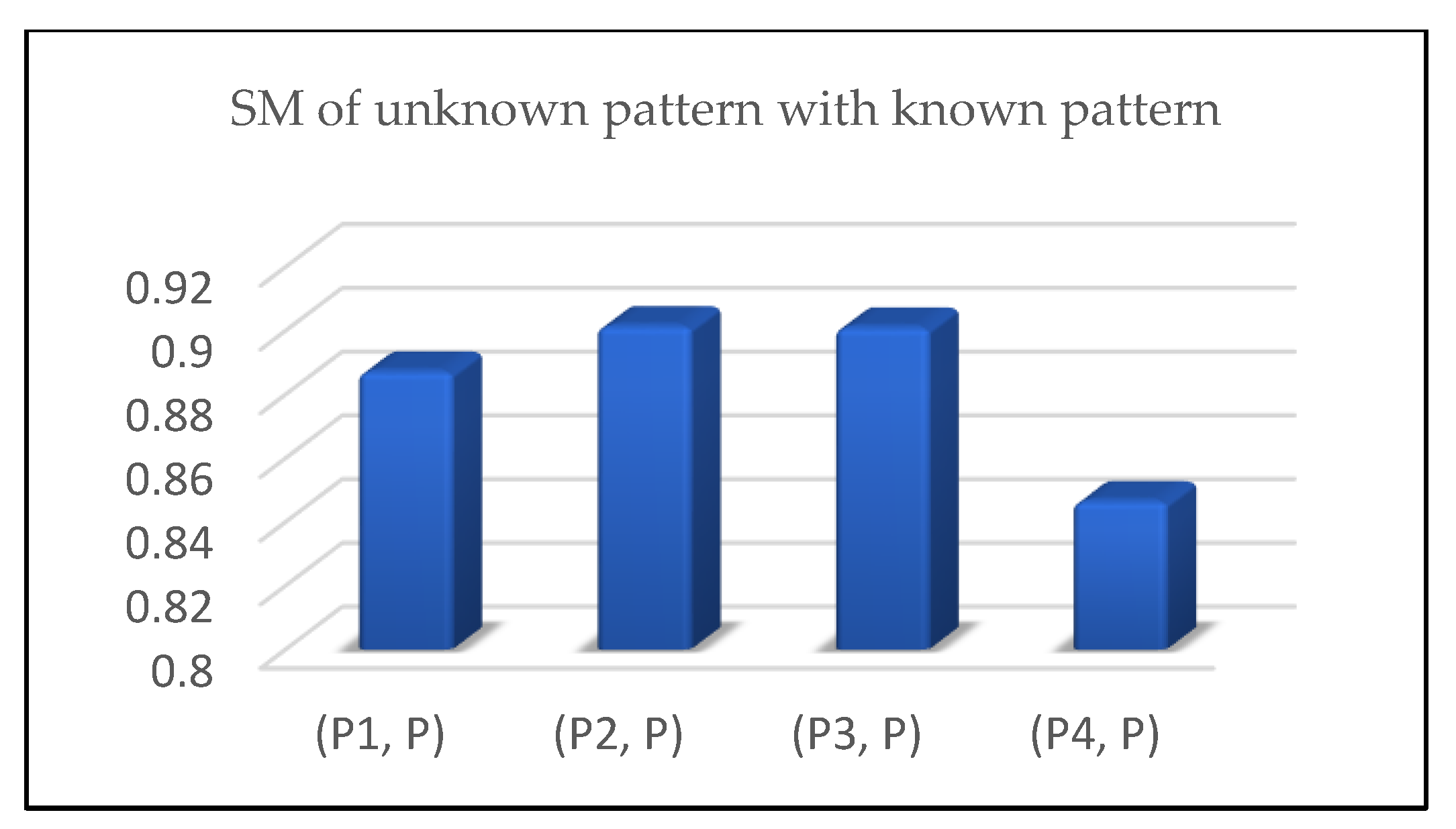
Step 3. Analyzing Table 2, we conclude that

$$\left({\mathrm{P}}_4, \mathrm{P}\right)<\left({\mathrm{P}}_1, \mathrm{P}\right)<\left({\mathrm{P}}_3, \mathrm{P}\right)<\left({\mathrm{P}}_2, \mathrm{P}\right)$$

As a result, the material ${\mathrm{P}}_2$ is nearest to $\mathrm{P}$ because the SM of $\left({\mathrm{P}}_2, \mathrm{P}\right)$ is greater than all the other pairs. Consequently, it is concluded that the unidentified material $\mathrm{P}$ corresponds to the ${\mathrm{P}}_2$ category of material. The results of Table 2 are also portrayed in Figure 1 where it shows that the unknown pattern $\mathrm{P}$ is closed to ${\mathrm{P}}_2$. The results also show that the unknown pattern $\mathrm{P}$ is still sufficiently close to the pattern ${\mathrm{P}}_3$ as well.

5.2. Comparative Study

In this section, we make comparisons of the results using the proposed SM for TSFSs with the results using the SM for TSFSs proposed by Ullah et al. [26] and Wu et al. [33].

Table 3. Comparative Study.

SM	Environment	Results
The proposed SM for TSFSs	TSFSs	$\left({\mathrm{P}}_4,\mathrm{P}\right)<\left({\mathrm{P}}_1,\mathrm{P}\right)<\left({\mathrm{P}}_3,\mathrm{P}\right)<\left({\mathrm{P}}_2,\mathrm{P}\right)$
The SM for TSFSs by Ullah et al. [25]	TSFSs	$\left({\mathrm{P}}_4,\mathrm{P}\right)<\left({\mathrm{P}}_3,\mathrm{P}\right)<\left({\mathrm{P}}_1,\mathrm{P}\right)<\left({\mathrm{P}}_2,\mathrm{P}\right)$
The SM for TSFSs by Wu et al. [32]	TSFSs	$\left({\mathrm{P}}_4,\mathrm{P}\right)<\left({\mathrm{P}}_1,\mathrm{P}\right)<\left({\mathrm{P}}_3,\mathrm{P}\right)<\left({\mathrm{P}}_2,\mathrm{P}\right)$

summarizes the findings. We find that the results using the proposed SM for TSFSs are the same as the results using the SM for TSFSs proposed by Wu et al. [33]. Here, we also show the limited nature of IFSs and PFSs. A brief comparison of the current paper’s aggregated results with those of other previous papers is provided in Table 3.

5.3. Applications for Decision Making

Now we will discuss how the proposed SM can be used to make decisions. The bigger the SM, according to the SM principle, the more correct the decision.

Example 2.

We use the proposed SM to solve the decision-making challenge proposed in Ullah et al. [34]. Islamabad, Pakistan’s capital, is regarded as one of the most beautiful cities in the world. There are various parks and picnic areas in Islamabad where a large number of people visit on a daily basis. The Metropolitan Corporation of Islamabad (MCI) is in charge of the city government. To maintain its appeal, the MCI decided to restore all of the parks and picnic areas. MCI will need to recruit some private contractors to do so. MCI chose four private firms for further consideration after some preliminary screening.${\mathsf{Á}}_1$: Arish Associates,${\mathsf{Á}}_2$: Nauman Estate and Builders,${\mathsf{Á}}_3$: Areva Engineering, Construction and Interiors, and${\mathsf{Á}}_4$: The Wow Architects, are among the four firms. MCI’s specialists devised five point criteria for selecting the best corporation or company.${\mathsf{Ҫ}}_1$: Cost,${\mathsf{Ҫ}}_2$: Previous performance,${\mathsf{Ҫ}}_3$: Time constraint,${\mathsf{Ҫ}}_4$: Quality assurance, and${\mathsf{Ҫ}}_5$: Labor quantity, are the five criteria. The decision-making panel has given all the information in TSFNs which is given in Table 3. The followings are the designated steps for the decision-making algorithm:

Step 1. Decision-makers’ views are expressed in the form of TSFNs, as indicated in

Table 4. Data on decision making.

	${\mathsf{Ҫ}}_1$			${\mathsf{Ҫ}}_2$			${\mathsf{Ҫ}}_3$			${\mathsf{Ҫ}}_4$			${\mathsf{Ҫ}}_5$
${\mathsf{Á}}_1$	0.1	0.7	0.4	0.5	0.8	0.9	0.8	0.8	0.8	0.6	0.7	0.8	0.3	0.5	0.7
${\mathsf{Á}}_2$	0.2	0.7	0.6	0.6	0.7	0.8	0.3	0.7	0.7	0.1	0.7	0.9	0.4	0.6	0.8
${\mathsf{Á}}_3$	0.5	0.6	0.6	0.5	0.6	0.7	0.5	0.7	0.1	0.9	0.6	0.2	0.5	0.6	0.9
${\mathsf{Á}}_4$	0.5	0.6	0.8	0.8	0.7	0.4	0.8	0.7	0.3	0.6	0.6	0.1	0.8	0.4	0.4
$\mathsf{Ҫ}$	1	0	0	1	0	0	1	0	0	1	0	0	1	0	0

.

Step 2. The SM of each TSFN given in Table 4 are evaluated with $\mathsf{Ҫ}\left(1,0,0\right)$ based on Equation (1).

Table 5. SM of ${\mathsf{Á}}_{ї}$ with $\mathsf{Ҫ}.$

SM	$\left({\mathsf{Á}}_1,\mathsf{Ҫ}\right)$	$\left({\mathsf{Á}}_2,\mathsf{Ҫ}\right)$	$\left({\mathsf{Á}}_3,\mathsf{Ҫ}\right)$	$\left({\mathsf{Á}}_4,\mathsf{Ҫ}\right)$
Values	0.5110507	0.3707117	0.5988922	0.7403513

summarizes the findings.

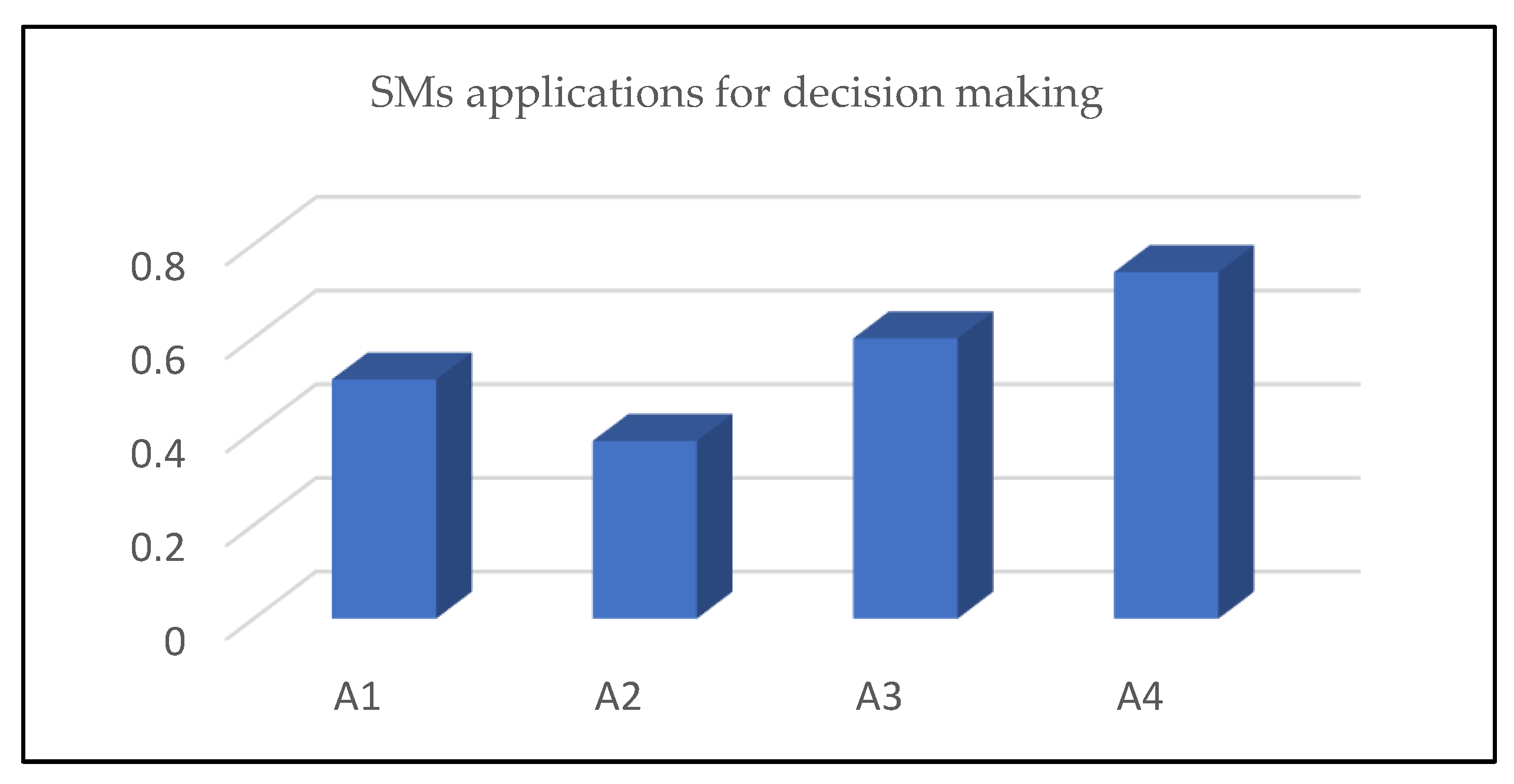
Step 3. Analyzing Table 5, we obtain

$${\mathsf{Á}}_2<{\mathsf{Á}}_1<{\mathsf{Á}}_3<{\mathsf{Á}}_4.$$

Therefore, ${\mathsf{Á}}_4$ is the best choice. The results of Table 5 are also shown in Figure 2 which indicates that, after applying the proposed SM, ${\mathsf{Á}}_4$ should be the best choice.

The findings of the proposed SM for TSFSs are then compared to the results of the SMs for TSFSs proposed by Ullah et al. [34].

Table 6. Comparative Study.

SM	Environment	Results
The proposed SM for TSFSs	TSFSs	${\mathsf{Á}}_2<{\mathsf{Á}}_1<{\mathsf{Á}}_3<{\mathsf{Á}}_4$
The SM for TSFSs by Ullah et al. [29]	TSFSs	${\mathsf{Á}}_2<{\mathsf{Á}}_1<{\mathsf{Á}}_3<{\mathsf{Á}}_4$

summarizes the findings. We find that both methods give the same decision.

6. Conclusions

In this paper, a new SM was presented for TSFSs which is based on DM, DA, and DNM. We had shown that the proposed SM for TSFSs satisfies the axiom of SM. It was also observed that the proposed SM provides a flexible and larger range for data representation under uncertain circumstances in which it can be a generalized SM for IFSs, PyFSs, PFSs, or SFSs. By using numerical examples, it was shown that the presented SM is more efficient and can provide accurate results as the information under consideration was based on TSFNs where more than two aspects of uncertain information were discussed. In addition, we applied the proposed SM in pattern recognition and decision-making to observe its effectiveness. The comparative studies on pattern recognition and decision making indicate that the proposed SM is valid and can be used in some real-life problems, especially in decision making, pattern recognition, and clustering. In general, symmetric triangular fuzzy numbers can be well used in database acquisition and so our further work shall first consider the proposed SM for symmetric T-spherical triangular fuzzy numbers. In our future works, we will also extend the proposed SM for interval valued TSFSs and complex TSFSs. We shall further develop new distances for TSFSs and give more entropy measures for TSFSs and then apply them in clustering and medical diagnosis problems under TSFSs environment.