
Mixtures of Semi-Parametric Generalised Linear Models


Department of Statistics, University of Pretoria, Pretoria 0002, South Africa
*
Author to whom correspondence should be addressed.
†
These authors contributed equally to this work.
Symmetry 2022, 14(2), 409; https://doi.org/10.3390/sym14020409
Submission received: 19 January 2022
/
Revised: 5 February 2022
/
Accepted: 15 February 2022
/
Published: 18 February 2022
(This article belongs to the Special Issue Symmetry in Multivariate Analysis)
Abstract
:The mixture of generalised linear models (MGLM) requires knowledge about each mixture component’s specific exponential family (EF) distribution. This assumption is relaxed and a mixture of semi-parametric generalised linear models (MSPGLM) approach is proposed, which allows for unknown distributions of the EF for each mixture component while much of the parametric structure of the traditional MGLM is retained. Such an approach inherently allows for both symmetric and non-symmetric component distributions, frequently leading to non-symmetrical response variable distributions. It is assumed that the random component of each mixture component follows an unknown distribution of the EF. The specific member can either be from the standard class of distributions or from the broader set of admissible distributions of the EF which is accessible through the semi-parametric procedure. Since the inverse link functions of the mixture components are unknown, the MSPGLM estimates each mixture component’s inverse link function using a kernel smoother. The MSPGLM algorithm alternates the estimation of the regression parameters with the estimation of the inverse link functions. The properties of the proposed MSPGLM are illustrated through a simulation study on the separable individual components. The MSPGLM procedure is also applied on two data sets.
1. Introduction
In many situations, mixture of regression modelling focuses on Gaussian distributions, and hence symmetrical component distributions [1,2]. Frequently, data follow a distribution that is non-standard, e.g., non-symmetric or skewed multi-modal. The flexibility embedded in mixture modelling based on known component distributions enables the modelling of both symmetric and non-symmetric data patterns. In many applications, the individual component distributions are of importance, and the selection of appropriate component distributions are essential. In the case of MGLM, both the selection of the correct component distribution members and the selection of the component link functions are required. Azzalini et al. [3] and Wainer [4] presented examples for a single component model, highlighting the inadequacy of using the typical logistic link to model binary responses. Weisberg [5] argued that if the chosen distributions are inadequate, a better fit might be obtained if the inverse link function is estimated from the data. Estimating the inverse link function directly from the data enables more flexible models. The proposed semi-parametric procedure for estimating the component inverse link functions facilitates the selection of component members from the broader class of EF distributions. Finite mixture modelling provides a statistical modelling approach with applications in a wide variety of random phenomena, including marketing and market segmentation [6], insurance [7], biology [8], medicine [9], and economics [10]. Recently, there has been an enhanced focus on non-parametric and semi-parametric mixture models. In 2019, Xiang, Yao, and Yang [11] published an overview of semi-parametric extensions of finite mixture models, and in 2020, Ma, Wang, and Lee [12] considered semi-parametric mixture regression with unspecified error distributions.
In this paper we start by considering MGLM [13,14], proposing a semi-parametric estimation of the component inverse link functions for modelling the component conditional expected value of the response variable given explanatory variables. The proposed MSPGLM has several important advantages:
- A semi-parametric, estimated, component inverse link function assists in determining if a selected parametric component link function is appropriate to be used as a component link function;
- If the selected parametric component link function is inadequate, a better component fit can be obtained by estimating a semi-parametric component link function. Improved component fits will improve the overall fitted mixture model;
- Relaxing the assumption of a common component link function by estimating individual semi-parametric component link functions;
- In [5], it is shown that under fairly general conditions, consistent estimates of the component parameter directions are obtained.
The MSPGLM has limitations similar to that of the SPGLM. Since a scale and location factor can be absorbed into the component link functions, the estimated component regression coefficients estimate a direction in p dimensional space. The magnitudes of the estimated component regression coefficients can therefore not be directly related to component rates of change in the explanatory variables. However, ratios of the estimated component regression coefficients are useful indications of the relative impact of variables at the component level, which is analogous to the findings in [15].
The performance of the proposed MSPGLM is evaluated through a simulation study, evaluating the performance of the individual components that are separable within the overall procedure. The procedure is also implemented on a data set from an insurance company and on a South African COVID-19 data set.
The paper is structured as follows. Section 2 describes the SPGLM, followed by the MSPGLM. Section 3 gives simulation results of the SPGLM performance for continuous and categorical response variables. In Section 4 and Section 5, applications of the proposed MSPGLM procedure on insurance and COVID-19 data are given. Lastly, Section 6 contains a discussion of the results, conclusions, and possibilities for future research.
2. Materials and Methods
2.1. Semi-Parametric Mixture of Generalised Linear Models
The GLM is a generalisation of the mean regression model, selecting a distribution of the EF for the random component, Y, with the following density or mass function:
where is the cumulant function and a dispersion parameter. , with , and is a smooth and invertible link function; is the vector of explanatory or feature variables, and is the vector of regression parameters. It follows for the EF that:
The canonical inverse link function is [16].
The SPGLM considers cases where the random component is assumed to follow an unknown distribution from the EF. The inverse link function is therefore also unknown and needs to be estimated in addition to the regression parameters .
2.2. SPGLM Estimation
Consider a random sample of pairs for . Set , and =. Following from (2), we estimate the expected value using the Nadaraya–Watson weighted average in the focal point z, varying over the range of possible values:
with as the normalising constant. This approach uses a one-dimensional smoother obtained from the linear predictor in contrast to a full non-parametric approach requiring a p dimensional smoother.
We use an alternating estimation scheme [5] by first estimating using the Newton Raphson algorithm, followed by the estimation of the inverse link function.
Next, we derive the Newton Raphson update rule for . The likelihood function for is as follows:
with the following log-likelihood:
which simplifies for the canonical link function to:
Maximising using the Newton Rapshon algorithm yields the update rule for :
with , and For , we substitute the Nadaraya–Watson weighted average of (4) into (5).
The second derivative of is estimated using the following:
which is the derivative of , or
derived using (3) for a fixed value of the dispersion parameter .
Weisberg and Welsh [5] proposed to initialise the semi-parametric estimation procedure by selecting a suitable parametric GLM to obtain initial values for and the inverse link function. This parametric inverse link function is updated using the non-parametric estimate . In the following step, updated values for are determined using (5). The procedure is iterated until convergence, selecting h through the use of cross-validation. The proposed procedure for estimating the SPGLM is given in Algorithm 1.
| Algorithm 1 Semi-parametric generalised linear models (SPGLM) |
|
2.3. Mixture of Semi-Parametric Generalised Linear Models
Consider K components, each with an SPGLM structure with an unknown link function for . The expected value of the kth component is . The random variable Y is observed from mixture component k with probability . For an MSPGLM, the density or mass function is as follows:
with , as the regression parameters and as the mixing probabilities.
For a random sample of n pairs for , the complete data log-likelihood function is the following:
where the unobserved component membership matrix , with
The complete data log-likelihood is maximised using the Expectation Maximisation (EM) algorithm [17]. We start with a suitable parametric MGLM to obtain initial parameter estimates , initial inverse link functions , and the estimated responsibilities for the ith observation in component k, , as in Millard [18]. The component inverse link functions are updated using the Nadaraya–Watson weighted average (4), with the following responsibilities incorporated:
where
and . The second derivative is estimated using the following:
The update rule for is as follows:
with . The MSPGLM estimation procedure is summarised in Algorithm 2.
| Algorithm 2 Mixture of semi-parametric generalised linear models (MSPGLM) |
|
3. Simulation Study
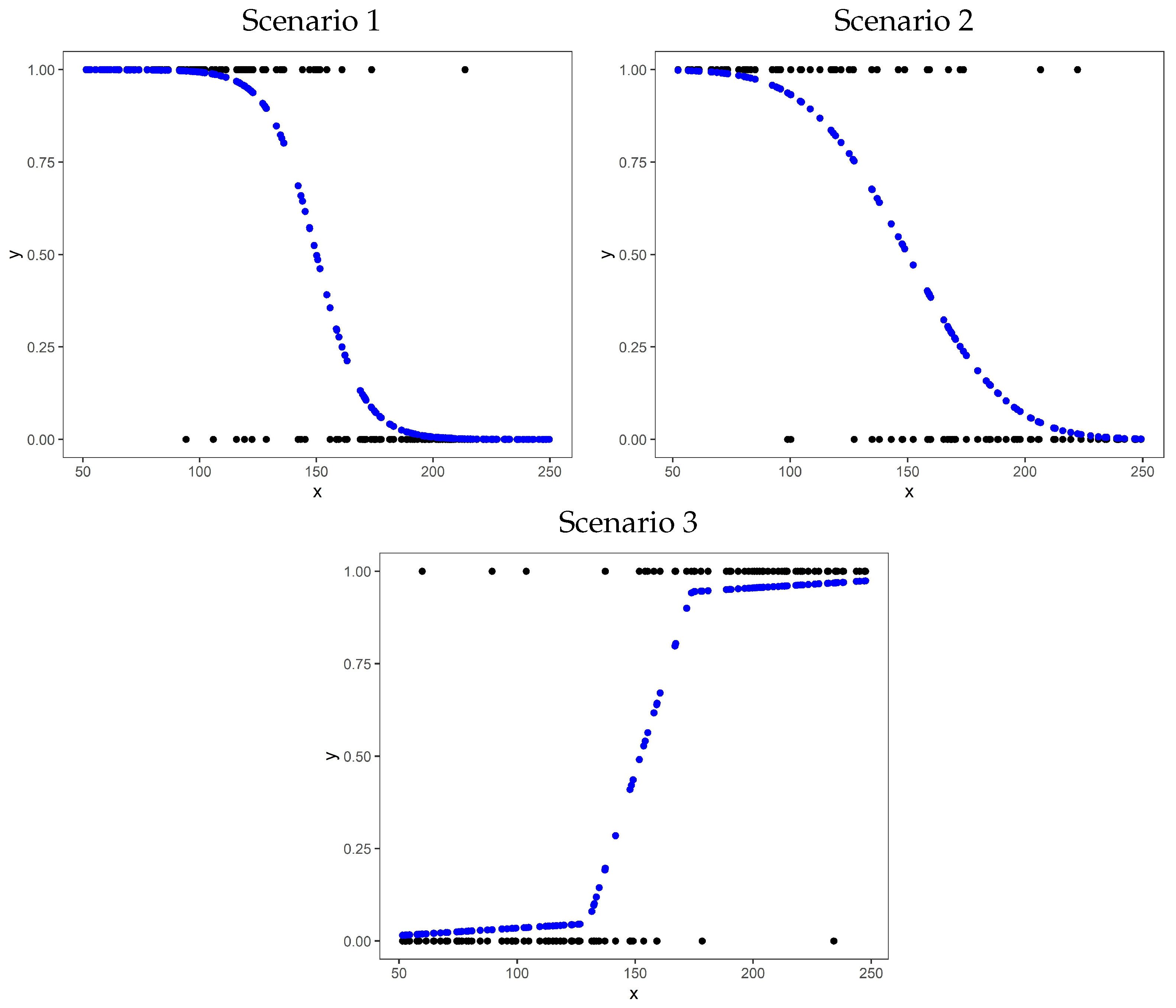
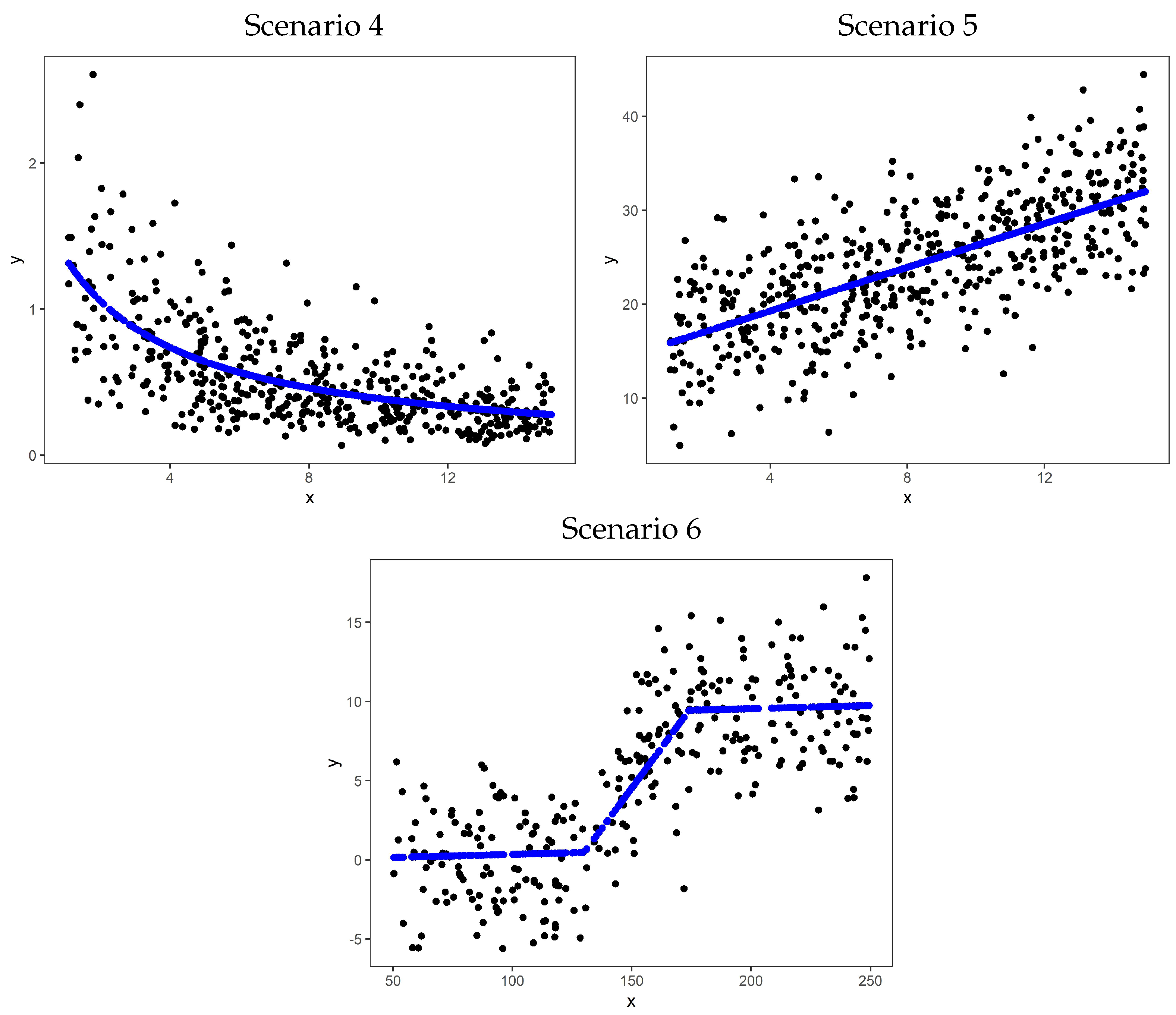
We assess the performance of the SPGLM estimation algorithm, Algorithm 1, in discrete and continuous scenarios considering different link functions and sample sizes. Data are generated using the specified link functions as indicated in Table 1. A GLM with a single feature variable is used in the generation. Scenarios 1–3 consider binary response models, with scenario 1 using a logit link. Scenarios 2 and 3 use the probit and piecewise linear link functions, respectively. Scenarios 4–6 are continuous response variable models using inverse, identity, and piecewise linear link functions.
A suitable GLM is fitted to the generated data to identify initial values for and an initial link function. The initial link functions are given in Table 1. The fitted model is obtained using Algorithm 1. Aligned to recent trends in simulation designs [19,20,21], this process is repeated 1000 times for each scenario. These simulation results also guide the MSPGLM since the mixture components are separable.
Figure 1 shows the inverse link functions used to generate the data and the response variable values for a single simulation iteration of the discrete response scenarios.
Similarly, Figure 2 shows the inverse link functions used to generate the data and the response variable values for a single simulation iteration of the continuous response scenarios.
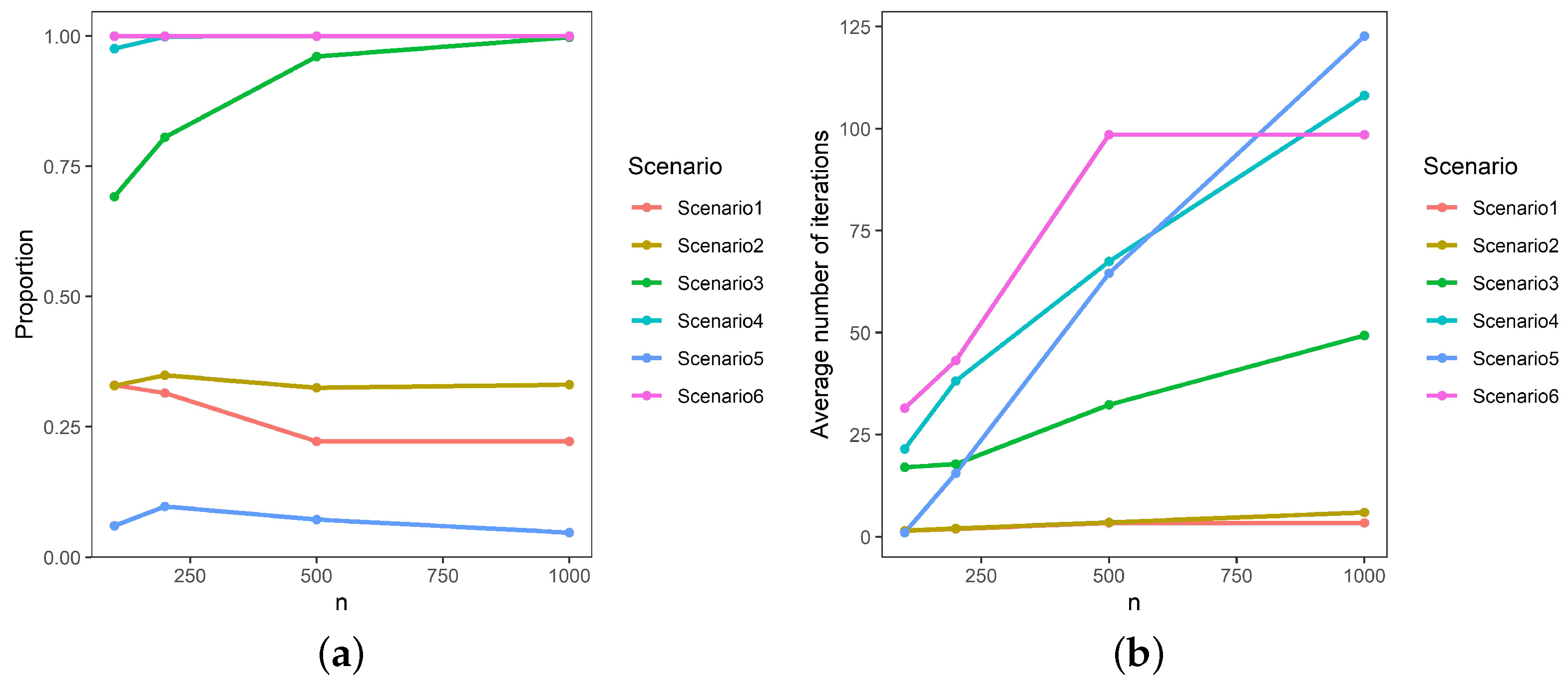
Table 2 gives the simulation results of the proportion of instances where the SPGLM procedure outperforms the initial link function based on the prediction error, which is also presented in the left pane of Figure 3. These scenarios clearly indicate the diverse results that can be obtained by the SPGLM. In scenario 1, the SPGLM outperforms the logit link function in – of the cases, with the lower percentages occurring as the sample size increases. This indicates that with larger sample sizes, the signal from the initial logit link function is of such a nature that the SPGLM procedure can only perform better in of the simulations. This low value is to be expected as the generation link function and the initial link function are the same. The SPGLM outperforms the logit link function for scenario 2 in – of the cases. This trend does not seem to change as the sample size increases. Scenario 3 shows that the prediction error decreases as the sample size increases. The SPGLM yields better results than the logit link function, varying between and as the sample size increases.
The SPGLM outperforms the inverse link function in scenario 4 in more than of the cases for all sample sizes evaluated. In scenario 5, the SPGLM only performs better in 4.5– of the cases. This is to be expected as the chosen initial link function is the link function that generated the data and therefore serves as confirmation of the parametric model. The piecewise linear link function, scenario 6, shows that the SPGLM outperforms the initial link function in all cases.
For scenarios 1 and 5, the SPGLM does not perform better than the initial link function. It can therefore be argued that the semi-parametric process is not able to identify a better inverse link structure compared to the parametric model under consideration, confirming the chosen initial link function as suitable. For scenarios 3, 4, and 6, the SPGLM generally outperforms the chosen initial link function, indicating the advantage of a data-driven link function. The estimated link function selects an unknown distribution from the broader class of distributions in the EF.
Table 3 gives the simulation results, based on the prediction error, of the number of iterations required for convergence in the cases where the SPGLM performs better than the initial link function, which is also shown in the right pane of Figure 3. The results are consistent in that the average number of iterations to convergence increases as the sample size increases.
This simulation study clearly illustrates the flexibility that can be achieved using the SPGLM procedure.
4. Application: Premium Collection Rates
4.1. Problem Statement and Data
This application is based on data received from a start-up insurance company. The company has 2227 active policies. Their target market is the lower income group. They market two unique products specifically designed to support the households of the policy holders in the event of a claim.
A major challenge in the insurance industry, specifically in the lower income bracket, is the premium collection rate. Collection rates in this market varies between and . The company is in need of a better understanding of the behaviour of its customer base and must use this understanding to focus their marketing efforts on customers in order to improve collection rates.
A model predicting the likelihood of a policyholder paying at least one premium in the next three months is required. The variables available are indicated in Table 4.
Relevant data were used to ensure that all policies are measured up to three months after the last month under consideration. A brief summary of the data is given in Table 5 and Table 6.
The exploratory results consider the marginal relationships between variables, not taking into account the differences between possible latent segments in the data. The section below considers an MSPGLM to model the collection rate. The identification of the latent segments will highlight differences in the regression structures, likely due to latent behavioural groups.
4.2. Modelling and Results
A two-component MSPGLM is fitted using the premium collection data. The estimated MSPGLM regression parameters are given in Table 7.
The parameters of the MSPGLM are not directly comparable to parametric MGLM parameters. We therefore use ratios of the regression parameters in Table 8 and Table 9 to determine the relative importance of the explanatory variables in components 1 and 2, respectively.
In both Table 8 and Table 9, the values above the diagonal of contain ratios indicating the relative importance of the parameters associated with the rows to parameters associated with the columns. Table 8 shows that for component 1, the variable Current had a contribution more than five times that of the variable Last3, and more than eight times that of Gender. Similarly, it can be seen that the relative importance of Bank-A is more than 160 times that of Bank-B. The corresponding importance for component 2 are and when comparing the variable Current to the variable Last3 and Gender, respectively, in Table 9. Comparing Bank-A to Bank-B yields a relative importance of , showing a different relationship when measuring the impact of the banks between components 1 and 2.
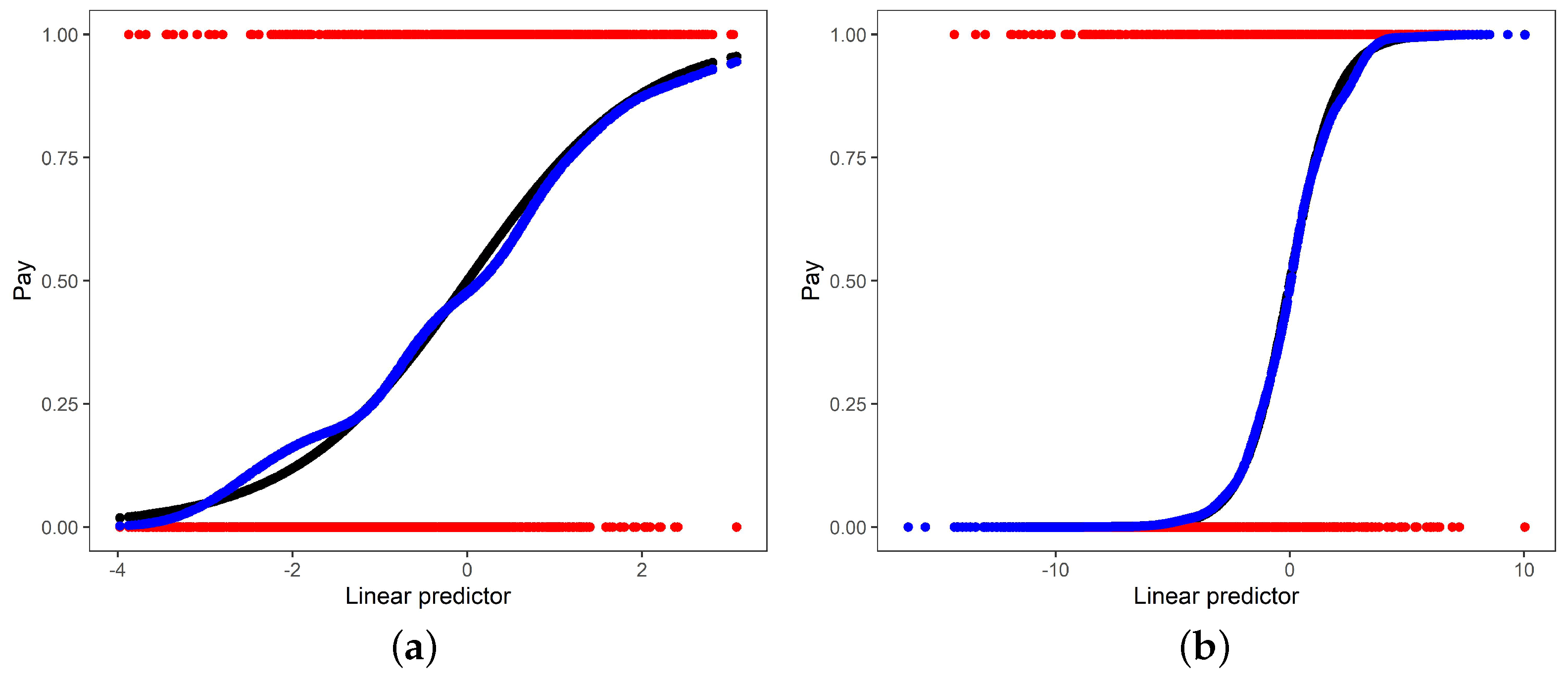
Figure 4 shows the estimated MGSPLM link function compared to the initial link function for component 1 in the left pane and for component 2 in the right pane. It is clear that the initial link, MGLM, and the MSPGLM link functions are similar, especially for component 2. This is supported by the prediction errors, as indicated in Table 10. In both components as well as overall, the MSPGLM performs marginally better than the MGLM model based on the initial link.
Table 11 gives the classification accuracy of the estimated MGLM and MSPGLM, respectively. The classification accuracy of both models are similar, with the MSPGLM again performing slightly better.
Given the marginal differences in the estimated inverse link functions of the MGLM and MSPGLM, the results support the use of the initial logit link function as the correct link function. The MGLM, a mixture of logistic regression models, could therefore be used as an appropriate model for the client retention application.
5. Application: COVID-19 Data
5.1. Problem Description and Data
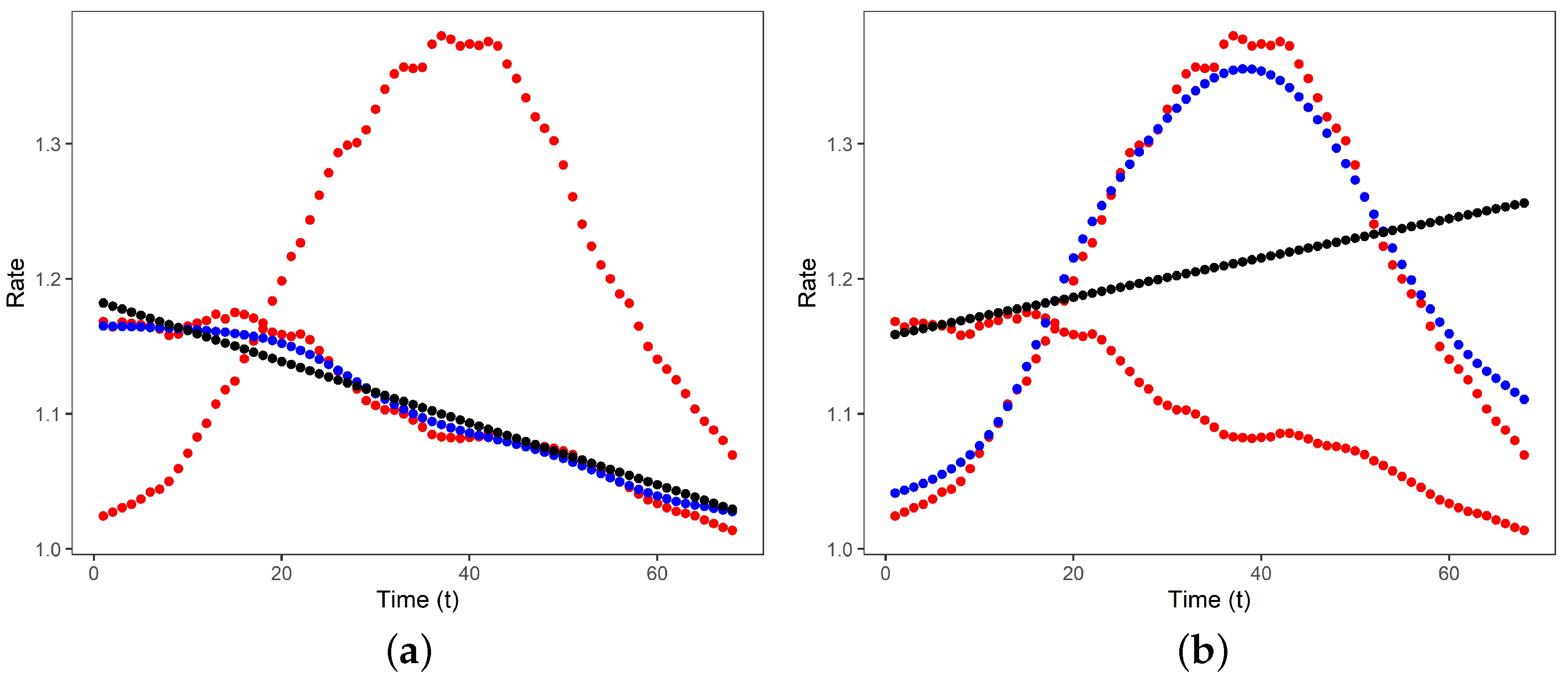
This section considers an application of MSPGLM to COVID-19 infection rates, with time as the explanatory variable. Data are observed for the Kwazulu-Natal and Eastern Cape provinces in South Africa. The response variable is the 14-day infection rate, calculated as , with as the daily cumulative COVID-19 positive cases in province p in time period t. This measure is useful in modelling the spread of the disease over time. We considered data spanning the period from December 2020 to 15 February 2021, which include the second wave of infections in South Africa. During this period, the 14-day infection rates varied between and , covering periods where the 14-day growth was almost stationary up to periods where the growth was more than 38%. The data were sourced from the Data Science for Social Impact COVID-19 data repository, hosted by the University of Pretoria.
5.2. Modelling and Results
A two-component MSPGLM is fitted to the COVID-19 14-day infection rate data, specifically to illustrate the ability of the estimation algorithm to update and improve the inverse link functions and to identify the latent provinces. Estimation Algorithm 2 is used to fit the MSPGLM model, selecting identity link functions as initial link functions and using only time as the explanatory variable in the linear predictor. The regression coefficients for the time variable, t, are and for the two components, respectively.
Figure 5 shows the observed data, initial inverse link functions as well as the estimated MSPGLM inverse link functions for both components, plotted against time. The components are identified using hard clustering.
It is clear that the mixture model could identify the two latent provinces. Based on the observed data, it is also clear that Eastern Cape has a downward sloping 14-day infection rate, while Kwazulu-Natal has a shape that increases and later decreases over the time period.
Figure 5 also clearly shows the ability of the estimation algorithm to update the initial inverse link functions to much more appropriate estimated inverse link functions. Component 1 is identified as the Eastern Cape and Component 2 as Kwazulu-Natal.
This improved fit of the MSPGLM is supported by the prediction errors in Table 12. In both components, the MSPGLM performs much better than the model based on the initial link functions.
The MSPGLM model therefore shows that the chosen initial link functions are not appropriate and that the estimated MSPGLM inverse link functions should rather be used.
6. Discussion and Conclusions
In this paper, we introduced an MSPGLM that estimates appropriate, semi-parametric component inverse link functions, which facilitates the selection of component members from the broader class of EF distributions. The approach allows for a more flexible modelling capability, resulting in an improved capturing of the observed structure.
The first derivative of the component cumulant function is the component inverse canonical link function, estimated using the Nadaraya–Watson weighted average. The MSPGLM procedure uses an alternating estimation scheme by first updating the component regression parameters, followed by updating the component inverse link function. The MSPGLM procedure either confirms the choice of the initial, parametric component inverse link function or estimates a component inverse link function from the broader class of distributions in the EF, resulting in a better model fit. These properties were explored in the simulation study.
The prediction accuracy in the simulation scenarios where the initial parametric link function was different from the generating link function was drastically improved by the MSPGLM, highlighting the value of the proposed data-driven semi-parametric procedure. This procedure outperformed the MGLM in 69.2– of the cases where the generating link function was substantially different from the initial parametric link function. The procedure also confirmed the suitability of the initial parametric link function in cases where the initial parametric link function corresponded to the generating link function.
Two practical applications were considered. The first application modelled premium collection rates in an insurance company. The estimation results confirm the logit component link functions as appropriate component link functions. In the second application, 14-day infection rates for COVID-19 were modelled. The estimated model improved the initial parametric link functions by updating the initial component identity link functions with estimated non-linear component link functions, showing a substantial improvement in the prediction accuracy. The latent provinces were also successfully identified.
Recent trends confirm a continued interest in a semi-parametric mixture regression, as indicated by [11]. Further research could include the development of an alternative approach to using the estimated regression parameters in order to simplify the interpretation thereof. Additionally, one could investigate different updating strategies for the responsibilities in the MSPGLM.
Author Contributions
Conceptualization, S.M.M. and F.H.J.K.; methodology, S.M.M. and F.H.J.K.; software, S.M.M.; formal analysis, S.M.M. and F.H.J.K.; writing—review and editing, S.M.M. and F.H.J.K.; visualization, S.M.M. and F.H.J.K.; project administration, S.M.M.; funding acquisition, S.M.M. and F.H.J.K. All authors have read and agreed to the published version of the manuscript.
Funding
This research was funded by STATOMET, the Bureau for Statistical and Survey Methodology at the University of Pretoria, grant number STM21a.
Institutional Review Board Statement
Not applicable.
Informed Consent Statement
Not applicable.
Data Availability Statement
Data used in the application are available in a publicly accessible repository.
Conflicts of Interest
The authors declare no conflict of interest.
Abbreviations
| EF | Exponential family |
| GLM | Generalised linear model |
| SPGLM | Semi-parametric generalised linear model |
| MGLM | Mixture of generalised linear models |
| MSPGM | Mixture of semi-parametric generalised linear models |
References
- An, P.; Wang, Z.; Zhang, C. Ensemble unsupervised autoencoders and Gaussian mixture model for cyberattack detection. Inf. Process. Manag. 2022, 59, 102844. [Google Scholar] [CrossRef]
- Huang, T.; Peng, H.; Zhang, K. Model selection for Gaussian mixture models. Stat. Sin. 2017, 27, 147–169. [Google Scholar] [CrossRef] [Green Version]
- Azzalini, A.; Bowman, A.; Härdle, W. On the use of nonoparametric regression for model checking. Biometrika 1989, 76, 1–12. [Google Scholar] [CrossRef]
- Wainer, H. Pyramid power: Searching for an error in test scoring with 830,000 helpers. Am. Stat. 1983, 37, 87–91. [Google Scholar]
- Weisberg, S.; Welsh, A.H. Adapting for the missing link. Ann. Stat. 1994, 22, 1674–1700. [Google Scholar] [CrossRef]
- Caracciolo, F.; Furno, M.; D’Amico, M.; Califano, G.; Di Vita, G. Variety seeking behavior in the wine domain: A consumers segmentation using big data. Food Qual. Prefer. 2022, 97, 104481. [Google Scholar] [CrossRef]
- Pacáková, V.; Zapletal, D. Mixture distributions in modelling of insurance losses. In Proceedings of the 2013 International Conference on Applied Mathematics and Computational Methods in Engineering, Sun Valley, ID, USA, 5–9 May 2013; pp. 16–19. [Google Scholar]
- Hamel, S.; Yoccoz, N.G.; Gaillard, J. Assessing variation in life-history tactics within a population using mixture regression models: A practical guide for evolutionary ecologists. Biol. Rev. 2017, 92, 754–775. [Google Scholar] [CrossRef] [PubMed]
- Kurz, C.F.; Hatfield, L.A. Identifying and interpreting subgroups in health care utilization data with count mixture regression models. Stat. Med. 2019, 38, 4423–4435. [Google Scholar] [CrossRef] [PubMed]
- Wang, E.; Lee, C. The impact of clean energy consumption on economic growth in China: Is environmental regulation a curse or a blessing? Int. Rev. Econ. Financ. 2022, 77, 39–58. [Google Scholar] [CrossRef]
- Xiang, S.; Yao, W.; Yang, G. An overview of semiparametric extensions of finite mixture models. Stat. Sci. 2019, 34, 391–404. [Google Scholar] [CrossRef] [Green Version]
- Ma, Y.; Wang, S.; Xu, L.; Yao, W. Semiparametric mixture regression with unspecified error distributions. Test 2020, 30, 429–444. [Google Scholar] [CrossRef]
- Jansen, R.C. Maximum likelihood in a generalized linear finite mixture model by using the EM algorithm. Biometrics 1993, 49, 227–231. [Google Scholar] [CrossRef]
- Nguyen, H.D. Finite Mixture Models for Regression Problems. Ph.D. Thesis, University of Queensland, St Lucia, Australia, 2015. [Google Scholar]
- Li, K.; Duan, N. Regression analysis under link violation. Annals Stat. 1989, 17, 1009–1052. [Google Scholar] [CrossRef]
- Dunn, P.K.; Smyth, G. Generalized Linear Models with Examples in R, 1st ed.; Springer: Berlin/Heidelberg, Germany, 2018. [Google Scholar]
- Dempster, A.P.; Laird, N.M.; Rubin, D.B. Maximum likelihood from incomplete data via the EM algorithm. J. R. Stat. Soc. Ser. B 1977, 39, 1–38. [Google Scholar]
- Millard, S.M. Contributions to Mixture Regression with Applications in Industry. Ph.D. Thesis, University of Pretoria, Pretoria, South Africa, 2018. [Google Scholar]
- Asar, Y.; Algamal, Z. A New Two-parameter Estimator for the Gamma Regression Model. Stat. Optim. Inf. Comput. 2022. [Google Scholar] [CrossRef]
- Belias, M.; Rovers, M.M.; Reitsma, J.B.; Debray, T.P.A.; IntHout, J. Statistical approaches to identify subgroups in meta-analysis of individual participant data: A simulation study. BMC Med. Res. Methodol. 2019, 19, 183. [Google Scholar] [CrossRef] [PubMed]
- Jia, B. The application of Monte Carlo methods for learning generalized linear mode. Biom. Biostat. Int. J. 2018, 7, 422–428. [Google Scholar]
Figure 1.
SPGLM discrete simulation cases, generated data, and inverse link functions for a single simulation iteration.
Figure 1.
SPGLM discrete simulation cases, generated data, and inverse link functions for a single simulation iteration.

Figure 2.
SPGLM continuous simulation cases, generated data, and inverse link functions for a single simulation iteration.
Figure 2.
SPGLM continuous simulation cases, generated data, and inverse link functions for a single simulation iteration.

Figure 3.
Proportion of cases (a) where the SPGLM outperforms the initial link, and the average number of iterations (b) until convergence versus sample size.
Figure 3.
Proportion of cases (a) where the SPGLM outperforms the initial link, and the average number of iterations (b) until convergence versus sample size.

Figure 4.
Observed data (red), the initial inverse link functions MGLM (black), and estimated MSPGLM inverse link functions (blue). Component 1 is presented in the left pane (a), with Component 2 in the right pane (b).
Figure 4.
Observed data (red), the initial inverse link functions MGLM (black), and estimated MSPGLM inverse link functions (blue). Component 1 is presented in the left pane (a), with Component 2 in the right pane (b).

Figure 5.
Observed data (red), the initial inverse link functions MGLM (black), and the estimated MSPGLM inverse link functions (blue). Component 1 is presented in the left pane (a), with Component 2 in the right pane (b). The first day of December 2020 corresponds to .
Figure 5.
Observed data (red), the initial inverse link functions MGLM (black), and the estimated MSPGLM inverse link functions (blue). Component 1 is presented in the left pane (a), with Component 2 in the right pane (b). The first day of December 2020 corresponds to .


Table 1.
Simulation scenarios considered for the SPGLM.
| Scenario | Response Type | Generating Link | Initial Link | Sample Sizes |
|---|---|---|---|---|
| 1 | Discrete | Logit | Logit | |
| 2 | Discrete | Probit | Logit | |
| 3 | Discrete | Piecewise linear | Logit | |
| 4 | Continuous | Inverse link | Identity | |
| 5 | Continuous | Identity | Identity | |
| 6 | Continuous | Piecewise linear | Identity |
Table 2.
Proportion of simulations where the SPGLM model outperforms the initial link, based on the prediction error, with standard deviations in brackets.
Table 2.
Proportion of simulations where the SPGLM model outperforms the initial link, based on the prediction error, with standard deviations in brackets.
| Response Type | Discrete | ||
|---|---|---|---|
| Scenario | 1 | 2 | 3 |
| Generating link | Logit | Probit | Piecewise linear |
| Initial link | Logit | Logit | Logit |
| Sample size | |||
| 100 | |||
| 200 | |||
| 500 | |||
| 1000 | |||
| Response Type | Continuous | ||
| Scenario | 4 | 5 | 6 |
| Generating link | Inverse | Identity | Piecewise linear |
| Initial link | Identity | Identity | Identity |
| Sample size | |||
| 100 | |||
| 200 | |||
| 500 | |||
| 1000 | |||
Table 3.
Average number of iterations until convergence, based on the prediction error, with standard deviations in brackets.
Table 3.
Average number of iterations until convergence, based on the prediction error, with standard deviations in brackets.
| Response Type | Discrete | ||
|---|---|---|---|
| Scenario | 1 | 2 | 3 |
| Generating link | Logit | Probit | Piecewise linear |
| Initial link | Logit | Logit | Logit |
| Sample size | |||
| 100 | |||
| 200 | |||
| 500 | |||
| 1000 | |||
| Response Type | Continuous | ||
| Scenario | 4 | 5 | 6 |
| Generating link | Inverse | Identity | Piecewise linear |
| Initial link | Identity | Identity | Identity |
| Sample size | |||
| 100 | |||
| 200 | |||
| 500 | |||
| 1000 | |||
Only the cases where the SPGLM outperforms the initial link.
Table 4.
Customer retention data available for modelling payment behaviour.
| Variable | Description | Role | Type |
|---|---|---|---|
| Pay (y) | A binary response variable indicating at least one payment in the following three months. | Response | Categorical |
| Current | A binary indicator of a payment in the current month. | Explanatory | Categorical |
| Last3 | The number of payments in the three months prior to the current month. | Explanatory | Numerical |
| Gender | Gender of the policy holder. | Explanatory | Categorical |
| Product | Product indicator (two products). | Explanatory | Categorical |
| Bank | Bank used for payments (4 banks). | Explanatory | Categorical |
| Age | Age of the policy holder during the month of evaluation. | Explanatory | Numerical |
Table 5.
Data summary: Age, Bank, and Gender versus Payment.
| Age | ||||
|---|---|---|---|---|
| Level | Frequency Non-Pay | Percentage Non-Pay | Frequency Pay | Percentage Pay |
| a:–24 | 88 | 65.185 | 47 | 34.815 |
| b:25–35 | 640 | 64.581 | 351 | 35.419 |
| c:35–45 | 526 | 65.504 | 277 | 34.496 |
| d:45–55 | 154 | 66.667 | 77 | 33.333 |
| e:55+ | 41 | 61.194 | 26 | 38.806 |
| Total | 1449 | 65.065 | 778 | 34.935 |
| Bank | ||||
| Level | Frequency Non-Pay | Percentage Non-Pay | Frequency Pay | Percentage Pay |
| A | 511 | 79.844 | 129 | 20.156 |
| B | 173 | 52.744 | 155 | 47.256 |
| C | 565 | 60.884 | 363 | 39.116 |
| D | 200 | 60.423 | 131 | 39.577 |
| Total | 1449 | 65.065 | 778 | 34.935 |
| Gender | ||||
| Level | Frequency Non-Pay | Percentage Non-Pay | Frequency Pay | Percentage Pay |
| Female | 625 | 62.189 | 380 | 37.811 |
| Male | 824 | 67.430 | 398 | 32.570 |
| Total | 1449 | 65.065 | 778 | 34.935 |
Table 6.
Data summary: Product and payment history versus Payment.
| Product | ||||
|---|---|---|---|---|
| Level | Frequency Non-Pay | Percentage Non-Pay | Frequency Pay | Percentage Pay |
| 0 | 686 | 70.143 | 292 | 29.857 |
| 1 | 763 | 61.089 | 486 | 38.911 |
| Total | 1449 | 65.065 | 778 | 34.935 |
| Current month payment indicator | ||||
| Level | Frequency Non-Pay | Percentage Non-Pay | Frequency Pay | Percentage Pay |
| 0 | 815 | 70.077 | 348 | 29.923 |
| 1 | 634 | 59.586 | 430 | 40.414 |
| Total | 1449 | 65.065 | 778 | 34.935 |
| Number of payments in the previous three months | ||||
| Level | Frequency Non-Pay | Percentage Non-Pay | Frequency Pay | Percentage Pay |
| 0 | 535 | 89.916 | 60 | 10.084 |
| 1 | 624 | 76.377 | 193 | 23.623 |
| 2 | 262 | 45.095 | 319 | 54.905 |
| 3 | 28 | 11.966 | 206 | 88.034 |
| Total | 1449 | 65.065 | 778 | 34.935 |
Table 7.
Estimated parameters of the MSPGLM model.
| Parameter Estimates | ||
|---|---|---|
| Variable | Component 1 | Component 2 |
| Current | 0.327 | 0.687 |
| Last3 | 0.063 | 0.357 |
| Gender | 0.040 | 0.025 |
| Product | 0.167 | 0.055 |
| Bank-A | −0.437 | −0.131 |
| Bank-B | −0.003 | 0.386 |
| Bank-C | −0.086 | 0.178 |
| Age | 0.011 | −0.030 |
Table 8.
Relative importance of the estimated regression parameters for component 1 of the MSPGLM.
| Variable | Current | Last3 | Gender | Product |
|---|---|---|---|---|
| Current | 1 | 5.160 | 8.161 | 1.961 |
| Last3 | 0.194 | 1 | 1.581 | 0.380 |
| Gender | 0.123 | 0.632 | 1 | 0.240 |
| Product | 0.510 | 2.632 | 4.162 | 1 |
| Bank-A | 1.334 | 6.887 | 10.890 | 2.617 |
| Bank-B | 0.008 | 0.042 | 0.066 | 0.016 |
| Bank-C | 0.264 | 1.363 | 2.155 | 0.518 |
| Age | 0.034 | 0.176 | 0.279 | 0.067 |
| Variable | Bank-A | Bank-B | Bank-C | Age |
| Current | 0.749 | 123.245 | 3.787 | 29.244 |
| Last3 | 0.145 | 23.883 | 0.734 | 5.667 |
| Gender | 0.092 | 15.103 | 0.464 | 3.584 |
| Product | 0.382 | 62.854 | 1.931 | 14.914 |
| Bank-A | 1 | 164.470 | 5.054 | 39.026 |
| Bank-B | 0.006 | 1 | 0.031 | 0.237 |
| Bank-C | 0.198 | 32.545 | 1 | 7.722 |
| Age | 0.026 | 4.214 | 0.129 | 1 |
Table 9.
Relative importance of the estimated regression parameters for component 2 of the MSPGLM.
| Variable | Current | Last3 | Gender | Product |
|---|---|---|---|---|
| Current | 1 | 1.923 | 27.097 | 12.565 |
| Last3 | 0.520 | 1 | 14.091 | 6.534 |
| Gender | 0.037 | 0.071 | 1 | 0.464 |
| Product | 0.080 | 0.153 | 2.157 | 1 |
| Bank-A | 0.191 | 0.368 | 5.18 | 2.402 |
| Bank-B | 0.562 | 1.080 | 15.225 | 7.060 |
| Bank-C | 0.260 | 0.500 | 7.040 | 3.264 |
| Age | 0.044 | 0.085 | 1.202 | 0.557 |
| Variable | Bank-A | Bank-B | Bank-C | Age |
| Current | 5.231 | 1.780 | 3.849 | 22.552 |
| Last3 | 2.720 | 0.926 | 2.001 | 11.728 |
| Gender | 0.193 | 0.066 | 0.142 | 0.832 |
| Product | 0.416 | 0.142 | 0.306 | 1.795 |
| Bank-A | 1 | 0.340 | 0.736 | 4.311 |
| Bank-B | 2.939 | 1 | 2.163 | 12.672 |
| Bank-C | 1.359 | 0.462 | 1 | 5.859 |
| Age | 0.232 | 0.079 | 0.171 | 1 |
Table 10.
Prediction errors for the MGLM and MSPGLM models.
| Component | MGLM | MSPGLM |
|---|---|---|
| Overall | 295.904 | 295.336 |
| Component 1 | 241.914 | 241.394 |
| Component 2 | 53.990 | 53.942 |
Table 11.
Classification accuracy for the MGLM and MSPGLM models.
| Model | Classification Acuracy |
|---|---|
| MGLM | |
| MSPGLM |
Table 12.
Prediction errors for the MGLM and MSPGLM models.
| Component | MGLM | MSPGLM |
|---|---|---|
| Overall | 7.706 | 1.736 |
| Component 1 | 1.144 | 0.819 |
| Component 2 | 6.562 | 0.917 |
Publisher’s Note: MDPI stays neutral with regard to jurisdictional claims in published maps and institutional affiliations. |
© 2022 by the authors. Licensee MDPI, Basel, Switzerland. This article is an open access article distributed under the terms and conditions of the Creative Commons Attribution (CC BY) license (https://creativecommons.org/licenses/by/4.0/).
Share and Cite
MDPI and ACS Style
Millard, S.M.; Kanfer, F.H.J. Mixtures of Semi-Parametric Generalised Linear Models. Symmetry 2022, 14, 409. https://doi.org/10.3390/sym14020409
AMA Style
Millard SM, Kanfer FHJ. Mixtures of Semi-Parametric Generalised Linear Models. Symmetry. 2022; 14(2):409. https://doi.org/10.3390/sym14020409
Chicago/Turabian StyleMillard, Salomon M., and Frans H. J. Kanfer. 2022. "Mixtures of Semi-Parametric Generalised Linear Models" Symmetry 14, no. 2: 409. https://doi.org/10.3390/sym14020409
Note that from the first issue of 2016, this journal uses article numbers instead of page numbers. See further details here.