An Integrated Framework Based on GAN and RBI for Learning with Insufficient Datasets

Abstract

Generative adversarial networks are known as being capable of outputting data that can imitate the input well. This characteristic has led the previous research to propose the WGAN_MTD model, which joins the common version of Generative Adversarial Networks and Mega-Trend-Diffusion methods. To prevent the data-driven model from becoming susceptible to small datasets with insufficient information, we introduced a robust Bayesian inference to the process of virtual sample generation based on the previous version and proposed its refined version, WGAN_MTD2. The new version allows users to append subjective information to the contaminated estimation of the unknown population, at a certain level. It helps Mega-Trend-Diffusion methods take into account not only the information from original small datasets but also the user’s subjective information when generating virtual samples. The flexible model will not be subject to the information from the present datasets. To verify the performance and confirm whether a robust Bayesian inference benefits the effective generation of virtual samples, we applied the proposed model to the learning task with three open data and conducted corresponding experiments for the significance tests. As the experimental study revealed, the integrated framework based on GAN and RBI, WGAN_MTD2, can perform better and lead to higher learning accuracies than the previous one. The results also confirm that a robust Bayesian inference can improve the information capturing from insufficient datasets.

1. Introduction

We have stepped into the era of AI for decades, and our generation has even been named the Big Data generation. However, we probably encounter fewer, small, and insufficient data available for decision-making, albeit usually requiring enough data to form reliable strategies amid rapid real-world changes. Insufficient datasets are often collected everywhere: by developing new products or new modules, modeling and detecting abnormal and unpredictable manufacturing problems [1,2,3,4,5], rare disease diagnoses [6,7,8], DNA analyses of cancer patients [9], etc. It is ironic that we can only collect rare data because of personal privacy in the data explosion age, but it is inevitable. In the real world, every company owns confidential data, such as medical data and banking data, and is prohibited by law to share them with the public. Another occasion when small samples are a problem is the processing of imbalanced datasets, as the data collected are extremely uneven among each class. Moreover, the modeling process based on imbalanced datasets would value the majority classes more highly and ignore the information from the minority classes, thereby yielding potentially biased results [10,11,12].

For the learning tasks with small or insufficient datasets, we proposed a method to generate more reliable virtual data. In the proposed method, we integrated the robust Bayesian inference and the mega-trend-diffusion method to establish a robust estimation of unknown population for the small dataset and adopted the Wasserstein Generative Adversarial Network, which can imitate the original dataset as closely as possible, as the implementation tool, to monitor the virtual sample generation process. The main contribution of this study is to propose a method to generate more informative virtual samples for small datasets, which can help improve the learning accuracy when conducting learning tasks with small datasets that contain insufficient information.

Insufficient datasets, with insufficient data size and imbalanced amounts among classes, lead to information asymmetry and compromise the model fit. When the trained model results from an insufficient dataset, it is expected that the overfitting model will have lower training errors and higher test errors. In addition, it is expected that the model will not work well in the real world. To make machine learning more reliable and robust, the first task should be to address the information asymmetry issue, the information gap between insufficient datasets and real data. In other words, it is possible to explore the underlying distribution of insufficient data and to estimate it as reasonably as possible, although we cannot make up for non-existent information.

When tackling the issue of insufficient datasets, artificially generating more data is an intuitive solution. It is the case, for example, of the Bootstrapping method [13]. The results of machine learning depend on the representative sample of data when implementing Bootstrapping. Furthermore, these kinds of intuitively generating methods are subject to important assumptions, like the independence of samples and a large enough sample size. The apparent simplicity and intuition may conceal the weakness of the original small datasets. The distribution underlying the insufficient datasets should possess the information requested by sample generating. Instead of repeating samples or other bootstrapping-like methods, generating data from an underlying distribution estimated from insufficient data would be more acceptable.

Virtual sample generation (VSG) is one solution for addressing the issues of learning with small sample data and insufficient datasets. It aims to exhaust the information from the insufficient datasets for estimating the underlying distribution to infer the possible population. Furthermore, VSG generates new data, named virtual samples, based on the estimated distribution, instead of resampling from the insufficient datasets. The distribution mentioned in the article does not mean the statistical distribution, but the functional distribution referring to the range according to which the population can be distributed. The VSG method provides an alternative way of learning with small datasets, while often raising another issue—namely, that the quality of the virtual samples produced is not stable and varies depending on the sample-generating algorithm adopted. If a biased generated virtual sample is obtained, the result of the subsequent modeling would be biased. Generative adversarial networks (GANs) [14] have been a popular VSG method, which consists of two parts—the generative network, known as Generator, and the discriminative network, known as Discriminator. The Generator is used to generate new data with a distribution like that of the original real data, so that the Discriminator is unable to distinguish them from the dataset of the original mixing and the generated data. The confrontation between the Generator and the Discriminator is the core concept of GAN, to ensure that the generated virtual samples are more like the training samples. Moreover, it is interesting that the VSG process of GAN does not really aim to handle the learning with small datasets, but usually to imitate the target image by generating mass virtual data, like the followed revisions (Wasserstein GAN (WGAN) [15], conditional GAN (GAN) [16]). Although the GAN and its extension versions enhance the similarity between generated virtual samples and real data, the need for vast amounts of data and heavy computational ties make the training costs unaffordable.

The previous research [17] proposed the improved GAN architecture, named WGAN_MTD, for the learning task with small numerical datasets. It integrated the mega-trend-diffusion (MTD) method and the generative network of GAN to construct an acceptable learning framework for small dataset learning. This framework makes the learning task more feasible when only insufficient data are available. The MTD method provides a new way to exhaust the last information of the small dataset through rebuilding the possible, estimated distribution for the small datasets on hand based on fuzzy theory. It addresses the data consumption issue in the training process of GAN, to a certain extent. To assure the stabilization of the learning performance resulting from MTD and make the learning framework more applicable to small datasets, we introduce the Bayesian technique to improve the modeling of small datasets’ estimated distributions. Bayesian inference allows researchers to combine subjective information or domain knowledge with the model establishment, when there is a lack of sufficient data for reliable modeling. Robust Bayesian inference (RBI) can help the extraction of information about the estimated distribution from small datasets and then avoid, as much as possible, the biased inference—in the form, for example, of learning results—coming from the insufficient datasets. This study aims to propose a machine learning framework capable of this robustness and of handling the insufficient datasets.

In the following sections, the Literature Review (Section 2) discusses several concepts and research articles related to the current topic. Our proposed approach to improving the MTD method and integrating it with the generative network of GANs is presented in Section 3. The integrated learning framework proposed was validated based on experiments with two public datasets, as presented in Section 4. Section 5 concludes the research and provides a summary.

2. Literature Review

2.1. Virtual Sample Generation

Since small data sizes limit the ability of modeling, especially for machine learning tools, ill-performance makes the modeling based on small datasets unsuitable for solving real-world problems. As mentioned above, VSG can intuitively generate virtual samples meeting the data required for most training processes and learning tools, and guarantee that the derived data follows the estimated distribution of original small datasets. In pattern recognition, VSG helps to solve the lack of training samples. Niyogi et al. [18] converted 2D images into 3D images by transforming mathematical algorithms. The generated virtual samples follow statistical inference mechanisms and the principle of repeated sampling without replacement. In industrial contexts, VSG tries to explore the possible range of manufacturing data and extends the basis of decision-support for rapid strategy-making to react to changing business challenges. Li et al. [19] produced a functional virtual population (FVP) through trial-and-error methods. This approach is the first method proposed for small dataset learning, and it aims to extend the domain of variables and generate virtual samples under the scenario of constructing early scheduling knowledge. It requires a trial-and-error procedure which takes time to complete [1]. When applying FVP to the system with nominal input variables or high covariance between time stages, it has significant limitations, keeping the modeling from converging toward a stable learning result [20].

To address the issue of insufficient information, the principle of information diffusion based on fuzzy theory provides VSG with a more robust and sufficient development [21]. Huang and Moraga [22] proposed the diffusion neural network based on the concept that each sample point following the normal diffusion function can be distributed or scattered on both sides of the center. This approach succeeded in raising the learning accuracy and improving the performance when learning with a small dataset. The information diffusion concept has been adopted in the development of the mega-trend diffusion (MTD) method. MTD was first proposed in [23] and considered to fill the information gap within the insufficient datasets based on the information diffusion method and fuzzy theory [21,24]. Unlike the information diffusion method, applying diffusion techniques to each data separately, MTD adopts the fuzzy-diffusion function to scatter a set of data across the entire dataset.

The above proposed method can improve the learning performance significantly when handling small datasets in the scenarios of less-heavy data consumption. When training the deep learning structure and facing huge amounts of data requirements, the amount of network parameters is much higher than the size of the data input.

2.2. Generative Adversarial Networks

A Generative Adversarial Network (GAN) [14] can be regarded as a type of machine learning framework composed of two mutually competing neural networks. With a given training dataset, GAN learns to generate new data with the same statistics as the training set, meaning that it follows the same distribution. In the application of image processing, a GAN trained on photographs can develop new photographs that are similar, at least superficially, to those produced by humans. Although GAN and its extension methods improve the similarity between the generated virtual sample and the real data, they mostly use a large number of graphic datasets as their input rather than small datasets of numeric data. Besides, the development of GAN is based on the convolutional neural network (CNN), which is a deep neural network (DNN) structure that is not suitable for learning scenarios with a sparse sample [25].

According to the website of GAN Zoo, more than 70 kinds of GAN are proposed and widely adopted in many fields. Mirza and Sander [16] proposed an improved version of GAN, conditional generative adversarial nets (can), subject to additional conditions of the generative/discriminative network. Besides, the improvement converted the GAN structure into a supervised learning model. Wasserstein GAN (WGAN) was proposed by Arjovsky et al. [15] and mainly improves the problem of gradient vanishing when adding the 1-Lipschitz continuous function, replacing the sigmoid function with the discriminative network and introducing the concept of Wasserstein Distance. As a result of these changes, the discriminative network output [0, 1] determines the degree of similarity to the training sample.

Li et al. [17] proposed a learning framework of GAN that can generate effective virtual samples with the small datasets, named WGAN_MTD. Based on the architecture of GAN, WGAN_MTD consists of a generative network for generating numerical data instead of graphical data, with leveraging MTD for virtual sample generation. It is developed based on the Wasserstein GAN (WGAN) architecture and modified mega-trend-diffusion (MTD), as the limitation of the generative network to control the VSG process.

2.3. Robust Bayesian Inference

In statistical inference, there are two mainstream philosophies: Bayesian and frequentist. Frequentist inference regards an unknown population with fixed, unvarying information. Based on this concept, researchers calculate confidence intervals for population parameters or significance tests of hypotheses [26]. Bayesian inference introduces Bayes’ theorem to update the probability of concerning hypotheses as more evidence or information becomes available. In the decision-making process, Bayesian inference depends closely on subjective probability, often defined by researchers or observers [27]. When the information from the data population is insufficient, Bayesian inference provides an alternative way to support the modeling of small datasets. Bayesian inference has been adopted in various fields, such as software development [28], medical diagnosis [29], civil engineering [30] and business negotiations [31]. It suggests that researchers consider leveraging subjective information or domain knowledge when they lack sufficient data for reliable modeling.

Robust Bayesian analysis (RBI) aims to explore the robustness of the inference obtained from the Bayesian analysis [32]. A robust inference means it does not vary sensitively by changing inputs and it depends more on the given subjective information. In RBI, researchers applied the Bayesian approach to all possible combinations of prior distributions functions, which are selected based on what they empirically consider reasonable. RBI provides an idea for extracting information about the population distribution from small datasets, with less influence from insufficient information on the population. Related research [33,34] shows that the learning performance can be acceptably improved by introducing RBI to the modeling process, and RBI can benefit small dataset learning by providing a robust information base for training the learning tools.

3. Learning Framework of Integrating RBI and GAN

3.1. Modified MTD with RBI

The ε-contaminated prior distribution of RBI has the following form:

$$\mathsf{\Gamma }=\left\{\pi :\pi =\left(1-\epsilon \right){\pi }_0\left(\theta |\mathsf{\lambda }\right)+\epsilon q, q\in Q\right\},$$

where ${\pi }_0\left(\theta |\mathsf{\lambda }\right)$ denotes the basic prior of parameter vector $\theta$ estimated with samples, λ is the hyperparameter vector, $q$ is a predefined contamination belonging to class $Q$, and ε means the extent of error in ${\pi }_0\left(\theta |\mathsf{\lambda }\right)$. The MTD framework depends totally on the computation based on the original dataset. For systematically controlling the risk behind the small dataset, we introduce the concept of RBI with $\epsilon$-level contamination to the MTD model. The controlling parameter, $\epsilon$, refers to any value between 1 and 0, used to express the error rate that could result from adopting the original dataset, and $\left(1-\epsilon \right)$ means the confidence level of believing the information from the original datasets. In the section, we modify the original MTD framework to acquire information from the collected data, but it is also reasonable to consider the subjective information from researchers.

By reshaping MTD, we first redefine each of its elements in terms of RBI as follows. In the MTD method, the location parameters of variable $X_j$ include its upper bound, $U{B}_j$, central location, $C{L}_j$, and lower bound, $L{B}_j$, which can form the parameter vector ${\theta }_j$ and ${\theta }_j=\left(L{B}_j,C{L}_j,U{B}_j\right)$. Moreover, $N_j^L$ and $N_j^U$ can be regarded as elements of the hyperparameter vector ${\mathsf{\lambda }}_j$, or ${\mathsf{\lambda }}_j=\left(N_j^L,N_j^U\right)$, which are used to compute the corresponding lower and upper bound, $L{B}_j$ and $U{B}_j$. $C{L}_j$, the center point of the range for variable $X_j$, can be found by averaging the minimum and the maximum value of $\left\{x_{1j}, x_{2j},\dots ,x_{nj}\right\}$, the data collected from size $n$, and it is involved with the formula computing of ${\theta }_j$ and ${\mathsf{\lambda }}_j$. Since this section aims to modify the MTD model, we adopt the same the form and formula of each element for ${\theta }_j$ and ${\mathsf{\lambda }}_j$, which can be referred to [17].

In the research, we take the same form of $L{B}_j,$ $C{L}_j$, $U{B}_j$, $N_j^L,$ and $N_j^U$, as suggested in [17]. Hence, $C{L}_j$ can be defined as the center point between the minimum and the maximum of values for the given $\left\{x_{1j}, x_{2j},\dots ,x_{nj}\right\}$, indicated as $mi{n}_j$ and $ma{x}_j$. The number of data that are less than, and greater than, $C{L}_j$ can be defined as $N_j^L$ and $N_j^U$, respectively, and $L{B}_j$ has the form as

$$L{B}_j=\left\{\begin{array}{c}min\left\{C{L}_j-\left(N_j^L/\left(N_j^L+N_j^U\right)\right)\sqrt{-2\left(s_j^2/N_j^L\right)ln\left({10}^{-20}\right)}, mi{n}_j\right\}\\ \\ mi{n}_j/5, s_j^2=0\end{array}\right.$$

(1)

In a large dataset, we would hardly ever get a sample variance of zero, i.e., $s_j^2=0$. However, this often occurs when processing a small dataset, and we need to define the value of $L{B}_j$ for that case. Analogous to $L{B}_j$, we set the form of $U{B}_j$ as

$$U{B}_j=\left\{\begin{array}{c}max\left\{C{L}_j-\left(N_j^U/\left(N_j^L+N_j^U\right)\right)\sqrt{-2\left(s_j^2/N_j^U\right)ln\left({10}^{-20}\right)}, ma{x}_j\right\}\\ \\ 5 ma{x}_j , s_j^2=0\end{array}\right.$$

(2)

Besides generating virtual samples, MTD constructs new variables that can produce more useful information for learning tools’ training, with membership function $MF$. When considering the RBI model, the membership function $MF$ can have the following form:

$$MF=\left(1-\epsilon \right)M{F}_0\left(\theta |\mathsf{\lambda } \right)+\epsilon q, q\in Q \mathrm{and} \epsilon \in \left(0, 1\right)$$

(3)

where $M{F}_0$ can be referred to the original form in [17], which is constructed with $\theta$ and $\mathsf{\lambda }$. Its membership value concerns a set of linear functions subject to the relative location of input $x_{ij}$, the ith data value of the jth variable. As Figure 1 shows, the triangle-shaped $M{F}_0\left(x_{i,j}\right)$ should consist of two linear functions concerning different cases of $x_{ij}$’s location: in the right side ($x_{ij}>C{L}_j$) and in the left side ($x_{ij}\le C{L}_j$). However, $M{F}_0$ is not necessarily a symmetric function, since $C{L}_j$ is not subject to $L{B}_j$ and $U{B}_j$, even if it looks like the center between them.

When integrating RBI, a $q$ function is introduced to the modified membership function $MF$, where $q$ can refer to any prior probability density form, such as a gaussian function with parameter $C{L}_j$ and sample variance $s_j^2$, $g$. Consequently, considering the ε-level of contamination with a gaussian prior $g$, the modified MTD has the ε-contaminated $MF$ formed as:

$$MF\left(x_{i,j}\right)=\left\{\begin{array}{cc}\left(1-\epsilon \right)\frac{x_{i,j}-L{B}_j}{C{L}_j-L{B}_j}+\epsilon g\left(C{L}_j, s_j^2\right),& if x_{i,j}\le C{L}_j\\ \left(1-\epsilon \right)\frac{U{B}_j-x_{i,j}}{U{B}_j-C{L}_j}+\epsilon g\left(C{L}_j, s_j^2\right),& otherwise\end{array}\right.$$

(4)

Supposing the researcher has come to know some specific characteristics unobserved from the small dataset on hand, the modified MTD model integrating RBI provides an operational $q$ to add certain subjective information. As the above $MF\left(x_{i,j}\right)$ shows, users can consider a symmetric gaussian prior $g$ and include it to $MF$ with a weight $\epsilon$, should $M{F}_0$ have a non-symmetric shape.

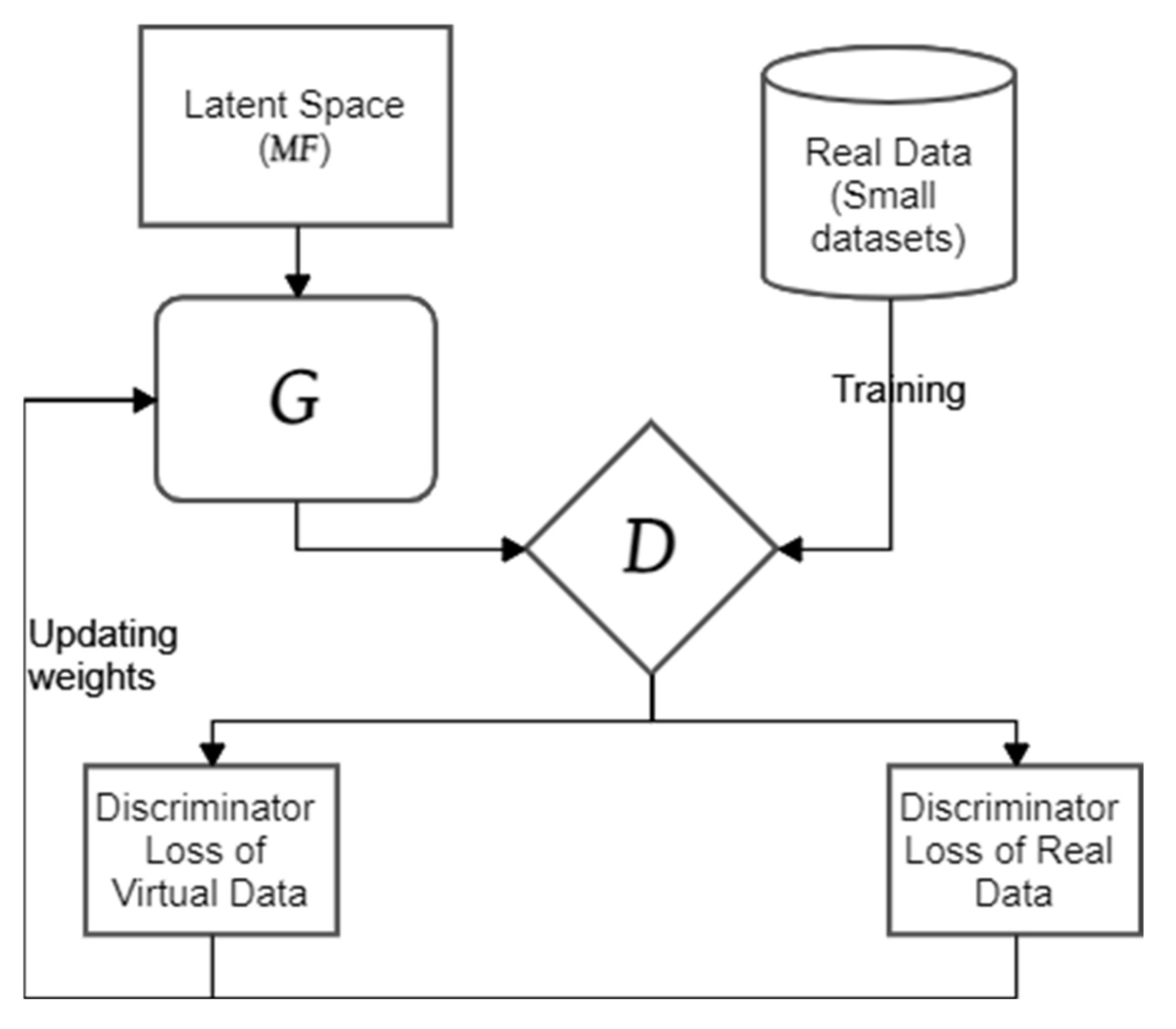
3.2. The Architecture of Modified WGAN_MTD

This study adopted the WGAN [15] as the basic adversarial architecture for further modification, in which the discriminating and generative networks take the back-propagation network as the training method, set the output layer activation function of output layers in the generative network to the tanh function, and propose the modified version of WGAN_MTD, named WGAN_MTD2. For the modified WGAN_MTD2, the WGAN determines whether the virtual sample, generated by the modified MTD (named MTD2), is like the real data, and then learns how to produce a set of virtual samples that resemble the original input more closely. The MTD2 limits the range of generated virtual samples with the mechanism consisting of RBI, including the data-driven $M{F}_0$ and a subjective prior $g$. The built-in RBI helps to minify the scope of virtual sample generation effectively, instead of irregularly producing virtual samples at the beginning of WGAN’s training. This is the main reason to integrate WGAN and MTD2 while applying the small-dataset learning.

The original purpose of GAN and its derivated WGAN is to solve the image problems of the real world by imitating the target image. When dealing with the numerical input, the generative-discriminative architecture must be modified accordingly. Furthermore, the original architecture adopts convolution neural networks (CNNs) as its discriminative and generative networks. The training process of CNNs requires heavy data consuming to tune the parameters and optimize the loss function that can be barely enough to achieve a stable learning result. Moreover, this is not feasible when applied to small datasets. In the research, the proposed architecture replaces the elements of CNNs with back-propagation networks (BPNs). Figure 2 shows the modified WGAN architecture adopting the BPN, requiring relatively less data for training processes, for setting both the generative and discriminative networks. When training the Discriminator, the discriminative network, the loss function consists of the loss in identifying real data and generated data instead of the original single network, so that the training of the discriminative network can be specific.

The modified MTD, MTD2, does make the training process of WGAN_MTD2 different from the previous WGAN_MTDs. Before inputting the training data into the modified architecture, we added an augmented variable, named Identifier, used to indicate a value of −1 for real data and 1 for the generated (virtual) sample. The new variable, Identifier, is designed to flag the input as real or generated, and the created information joins the training process for updating the parameters and tuning the corresponding loss function. As for the original design of generating random numbers from Latent Space, we specified Latent Space as the MTD2 in the modified version, so that it would turn to draw data from the estimated population constructed by MTD2 as the input for the following generative network and set the Identifier’s values of these virtual samples to 1.

The training of D, the discriminative network, takes both the ordinal, small data and the virtual data outputted by the Generator, the generative network, into account. The whole process will adjust, update, and tune the weights of the discriminative network by optimizing its loss function. The pathway including the Generator, the Discriminator, and both of the loss functions forms a training loop. This applies to random numbers generated from Latent Space, MTD2, and virtual generated samples with Generator. The corresponding Identifier values of these virtual samples are assigned a value of −1 when the training process has stabilized and learnt how to generate a set of virtual samples similar to the real data, meaning that the generated virtual data should look like they came from the same population as the real data. The above process will be operated iteratively until it meets the stopping rules, such as the set number of epoch and reaching the given threshold or the acceptable loss value. Then, the training task can be regarded as finished. It is expected that WGAN_MTD2 will entail less training costs then WGAN, because WGAN_MTD2 requires less data-consuming and light computational works.

We summarized the operating steps of WGN_MTD2 as follows:

Step 1: Estimate Latent Space for a virtual dataset with size $N;$ suppose a set of real data $X$ with size $n$ is given, by calculating $L{B}_j$ $C{L}_j$ $U{B}_j$ $N_j^L$ and $N_j^U$ with the formular mentioned above for each $X_j$, where $j=1,2,\dots ,m$.

Step 2: Construct the form of $MF\left(x_{i,j}\right)$ for $\left\{x_{i,j}\right|i=1,2,\dots ,N\}$ with a presetting $\epsilon$ and $g$ based on MTD2.

Step 3: Draw a random number $r$ from $\left\{\left(0,i\right)\right|i=1,2,\dots ,N\}$ iteratively and map these $N$ random numbers, $\left\{r_1,\dots ,r_N\right\}$, into $\left(L{B}_j,U{B}_j\right)$ by $\left\{v_{i,j}\right|i=1,2,\dots ,N\}$, where $v_{i,j}=L{B}_j+r_i\left(U{B}_j-L{B}_j\right), i=1,2,\dots ,N$

Step 4: Calculate the value of $MF$ for each point of the real dataset with size $n$ and $\left\{v_{i,j}\right|i=1,2,\dots ,N\}$, and obtain $n+N$ membership function values as the additional information, new variable, for original data $X$.

Step 5: Combine the data generated for each $X_j$, including the augmented new variable, based on the assumption of independence for the variables, for the virtual dataset.

Step 6: Train Generator of WGAN_MTD2 with the virtual dataset obtained from Step 5.

Step 7: Train Discriminator of WGAN_MTD2 with the output obtained from Step 6, the real dataset, and the corresponding values of the Identifier variable.

Step 8: Update weights and parameters iteratively until they meet the stopping rules.

4. Experimental Studies

By verifying the effectiveness of our proposed WGAN_MTD2, we conducted experiments to examine its performance. The section details the implementation of these experiments and the corresponding results, as well as the comparison with the previous version model, WGAN_MTD [17]. We used the same datasets as the inputs for both WGAN_MTD and WGAN_MTD2 to compare their performance, which enabled a fair judgement of whether the new version works better. Furthermore, we also compared its performance with those of other learning models, such as support vector machines (SVM), decision trees (DT), and naive Bayes classifiers (NBC). Public data sets from the UC Irvine Machine Learning Repository are adopted for our verification.

4.1. Evaluation Criterion

The criteria for the performance evaluation include the learning accuracy, standard deviation, and p-value of the significance test. Learning accuracy refers to how the virtual generated data perform subject to various prediction models, in particular to the models based on only considering small dataset inputs. We took the standard deviation and the p-value as the measurement of the consistency and stability of the experiments. For a given dataset as the input of different models, the smaller value of standard deviation means that the corresponding model can lead to higher stability and more reliable learning results. And a smaller p-value of significant tests shows that the differences of learning accuracies between various models can be more consistent. On the contrary, there might be no significant difference among the accuracies from various models if a higher p-value is shown, meaning the performance of compared models might not be far-off.

4.2. Experiment Environment and Datasets

To conduct the experiments, we adopted the Python integrated development environment in Anaconda, including the libraries Pandas, NumPy, Scikit-learn, and TensorFlow. All the tools mentioned above are open-sourced and available from the internet. When setting up the experimental environment, the hardware specification we selected includes an Intel Core i7 processor, 16 GB of RAM, and a NVIDIA GeForce GTX 1650 graphics chip. For verifying the model performances, three common learning tools, SVM, DT, and NBC (these abbreviations stand for Support Vector Machines, Decision Trees, and Naive Bayes Classifiers), are considered in the comparison with WGAN_MTD2 and WGAM_MTD. In the setting of SVM, two types of kernel functions are included: polynomial functions and radial basis functions (RBF). We included a scikit-learn library to perform learning tools’ training. When setting DT, we selected C5.0 as the training algorithm, since it uses less memory and builds smaller rulesets than C4.5 while being more accurate. When comparing the performances of various models, the learning processes are based on the same datasets, cited from UC Irvine Machine Learning Repository (UCI, Retrieved 15 June 2021, from https://archive.ics.uci.edu/). As

Table 1. Detail of datasets from UC Irvine Machine Learning Repository (UCI, Retrieved 15 June 2021, from https://archive.ics.uci.edu/).

Datasets	Total Samples	Input Attributes	Output Attributes	Number of Samples
				Class 1	Class 2	Class 3
Wine	178	13	1	59	71	48
Seeds	210	6	1	70	70	70
Cervical Cancer	72	18	1	21	51	-
Lung Cancer	32	55	1	9	13	10

shows, these datasets, Wine, Seeds, Cervical Cancer and Lung Cancer, are relatively small in sample size, from 32 to 210, with respect to the number of variables (input attributes), and from 6 to 55. All three datasets contain a single independent variable, the output variable, for classification.

4.3. Experiment Results

Table 2. The learning accuracies of 4 different models considering original small datasets (SDS) and virtual samples by WGAN_MTD and WGAN_MTD2, respectively (10 TD, Wine dataset).

Averaged Accuracy	SVM_poly	SVM_rbf	DT	NBC
SDS	55.323%	57.684%	68.171%	61.905%
WGAN_MTD	77.673% *	78.323% *	85.632%	74.271%
WGAN_MTD2	83.119% **,++	79.160% *,+	86.342% **,+	79.104% ***,++

* and ⁺ mean a p-value less than 0.05, ** and ⁺⁺ mean a p-value less than 0.01, *** mean a p-value less than 0.001.

lists various results of the virtual sample generated by WGAN_MTD2 based on the training datasets of size 10, referred to as 10 TD, from the Wine dataset. For every dataset, we repeated the experiments 30 times for each learning tool (SVM, DT, and NBC). As mentioned before, we considered SVMs of two different kernels; SVM_poly denotes SVMs with polynomial kernel functions, while SVM_rbf denotes SVMs with a radial basis function kernel. After training the learning tools and conducting a 10-fold cross-validation, we averaged the accuracies for each learning tool and each kinds of input. Table 2 shows averaged learning accuracies and a significance test result with considering p-values for each kind of experiment for the Wine dataset. For every learning model, the experiments include the training process based on training sets from three scenarios, meaning three kinds of inputs, with only the original small dataset (the Wine dataset cited for Table 2), with virtual samples generated by WGAN_MTD and WGAN_MTD2, respectively. To examine the effectiveness of the proposed method and how it works better than others, we compared the averaged accuracies resulted from three kinds of inputs, for each learning tool (SVM_poly, SVM_rbf, DT, and NBC). We denoted each kind of input as SDS, WGAN_MTD and WGAN_MTD2. SDS means that the learning tool will include only the original small dataset for training. WGAN_MTD and WGAN_MTD2 indicate that the learning tool will be trained with virtual samples generated by WGAN_MTD and WGAN_MTD2, respectively.

As to the comparison, we conducted the significance t tests with p-value for differences between SDS and WGAN_MTD, and differences between SDS and WGAN_MTD2. The star mark denotes the significance in statistics for different comparisons: * means a p-value less than 0.05, ** means a p-value less than 0.01, and *** means a p-value less than 0.001. We also conducted the significance t tests with p-value for differences between WGAN_MTD and WGAN_MTD2. The “+” mark denotes the significance in statistics for these comparisons: ⁺ means a p-value less than 0.05, ⁺⁺ means a p-value less than 0.01, and ⁺⁺⁺ means a p-value less than 0.001.

In Table 2, the experiments show that our proposed WGAN_MTD2 works better in these four models, as indicated by the better average accuracies and significance by the p-value (under 0.01) for 10 TD in the Wine dataset with 100 virtual data generated. The significance tests show that WGAN_MTD and WGAN_MTD2 improve the learning tools and lead to a better learning accuracy than SDS, both for SVM_poly and SVM_rbf. WGAN_MTD2 performs better than WGAN_MTD, both for SVM_poly and SVM_rbf, as the + marks imply. For DT and NBC, WGAN_MTD2 can help raise the learning accuracy higher than WGAN_MTD and SDS.

Further experiments were conducted with various amounts of training datasets (10, 15, and 20) in the Wine dataset. The sample size of virtual data generated was set to 100, for the aforementioned experiments, when applying WGAN_MTD and WGAN_MTD2 to each model.

Table 3. The experiment results of SDS, WGAN_MTD, and WGAN_MTD2 when generating 100 virtual samples for the Wine dataset.

Accuracy (%)		Learning Model
		SVM_poly			SVM_rbf			DT			NBC
		SDS	WGAN_MTD	WGAN_MTD2	SDS	WGAN_MTD	WGAN_MTD2	SDS	WGAN_MTD	WGAN_MTD2	SDS	WGAN_MTD	WGAN_MTD2
10 with 100 virtual samples	average	55.323	77.673	83.119	57.684	78.323	79.160	68.171	85.632	86.342	61.905	74.271	79.104
	Comparsion		*	**,++		*	**,+			**,+			***,++
15 with 100 virtual samples	average	70.319	80.849	86.421	72.438	80.077	82.109	73.119	84.371	86.231	75.125	81.903	80.111
	Comparsion		**	**,++			*,+		**	***,+		ns	*,+
20 with 100 virtual samples	average	75.369	82.263	85.157	77.069	85.512	86.287	74.731	83.132	84.781	79.709	80.739	82.246
	Comparsion		**	***,++		ns	*,+		**	***,++		ns	*,+

* and ⁺ mean a p-value less than 0.05, ** and ⁺⁺ mean a p-value less than 0.01, *** mean a p-value less than 0.001.

lists the averaged accuracies for each learning model trained by SDS, WGAN_MTD, and WGAN_MTD2, where each averaged value is calculated from 30 repeated experiment results. As Table 3 shows, WGAN_MTD2 provides a better performance for the four learning models listed when using only 10 training data as the virtual data generation seeds, and WGAN_MTD2 provides a better performance in averaged accuracy for SVM_ploy and DT when 15 training data are selected from the original Wine dataset as the seed to generate 100 virtual data, where the corresponding marks show the significant difference based on the p-value. Similarly, WGAN_MTD2 also results in higher averaged accuracies for SVM_ploy and DT when increasing the size of original data for virtual sample generation, such as a size of 20, where the corresponding marks show the significant difference based on the p-value.

For the Seed dataset, we conducted experiments using various amounts of training datasets (10, 15, and 20), considering 100 virtual generated data when applying WGAN_MTD and WGAN_MTD2 to each model. Using the layout of Table 3 and

Table 4. The experiment results of SDS, WGAN_MTD, and WGAN_MTD2 when generating 100 virtual samples for the Seed dataset.

Accuracy (%)		Learning Model
		SVM_poly			SVM_rbf			DT			NBC
		SDS	WGAN_MTD	WGAN_MTD2	SDS	WGAN_MTD	WGAN_MTD2	SDS	WGAN_MTD	WGAN_MTD2	SDS	WGAN_MTD	WGAN_MTD2
10 with 100 virtual samples	average	69.403	74.532	80.619	83.527	85.720	84.760	79.797	79.180	81.275	71.895	74.907	78.944
	Comparsion		*	**,++		ns	*,+		ns	+		*	**,++
15 with 100 virtual samples	average	72.785	80.171	82.219	87.303	87.711	86.809	82.018	82.191	84.233	81.837	82.328	82.191
	Comparsion		***	***,++		ns	ns		ns	*,+		ns	*,+
20 with 100 virtual samples	average	76.789	81.981	82.578	88.762	89.563	87.876	84.705	85.561	85.192	86.004	85.372	84.286
	Comparsion		**	***,++		ns	*		ns	ns		ns	*,+

* and ⁺ mean a p-value less than 0.05, ** and ⁺⁺ mean a p-value less than 0.01, *** mean a p-value less than 0.001.

, we list the averaged accuracies for each learning model trained by SDS, WGAN_MTD, WGAN_MTD2, where each averaged value is calculated from 30 repeated experiment results. As Table 4 shows, WGAN_MTD2 provides a better performance in the averaged accuracy for SVM_poly and NBC when using only 10 training data as the virtual data generation seeds to generate 100 virtual data for training. Besides, WGAN_MTD2 also works well for SVM_poly when increasing the size of the original Seed dataset, to 15 and 20. As for

Table 5. The experiment results of SDS, WGAN_MTD, and WGAN_MTD2 when generating 100 virtual samples for the Cervical Cancer dataset.

Accuracy (%)		Learning Model
		SVM_poly			SVM_rbf			DT			NBC
		SDS	WGAN_MTD	WGAN_MTD2	SDS	WGAN_MTD	WGAN_MTD2	SDS	WGAN_MTD	WGAN_MTD2	SDS	WGAN_MTD	WGAN_MTD2
10 with 100 virtual samples	average	70.593	75.391	82.953	84.771	84.953	83.701	73.184	76.453	80.372	70.462	72.682	80.944
	Comparsion		*	**,++		*	*,++		ns	*,+		*	**,++
15 with 100 virtual samples	average	74.963	81.224	84.829	86.921	88.761	87.139	80.253	81.741	83.723	79.937	81.592	82.143
	Comparsion		***	***,+++		*	ns		ns	*,++		*	*,+
20 with 100 virtual samples	average	75.971	82.891	83.816	87.267	88.938	87.943	83.535	86.171	84.982	80.922	82.782	83.736
	Comparsion		**	***,++		*	*		ns	ns		ns	*,++

* and ⁺ mean a p-value less than 0.05, ** and ⁺⁺ mean a p-value less than 0.01, *** and ⁺⁺⁺ mean a p-value less than 0.001.

, the experiments for the Cervical Cancer dataset show results similar to those from Table 4. The proposed WGAN_MTD2 provides a better performance in the averaged accuracies for the SVM_ploy and NBC and is even better than the results from the previous version, WGAN_MTD. Similarly, WGAN_MTD2 also works well for SVM_poly when increasing the size of the Cervical Cancer dataset with 100 virtual samples, to 15 and 20.

In the experiments for the Lung Cancer dataset, the proposed WGAN_MTD2 provides a better performance in averaged accuracies for SVM_ploy, SVM_rbf, DT, and NBC. By increasing the training data and virtual samples, the averaged accuracies is apparently raised for SDS, WGAN_MTD, and WGAN_MTD2. Furthermore, the averaged accuracies from WGAN_MTD2 are even better than the results from the previous version, WGAN_MTD. For the two cancer datasets, we demonstrated medical applications that, by applying WGAN_MTD2, can help the learning performance when dealing with the classification task. With the assistance of WGAN_MTD2, it can generate more informative virtual data as the input for learning tools and help them achieve better accuracies when classifying the cases of cancer. Moreover, the results from these four learning tools support this view.

From Table 3, Table 4, Table 5 and

Table 6. The experiment results of SDS, WGAN_MTD, and WGAN_MTD2 when generating 100 virtual samples for the Lung Cancer dataset.

Accuracy (%)		Learning Model
		SVM_poly			SVM_rbf			DT			NBC
		SDS	WGAN_MTD	WGAN_MTD2	SDS	WGAN_MTD	WGAN_MTD2	SDS	WGAN_MTD	WGAN_MTD2	SDS	WGAN_MTD	WGAN_MTD2
10 with 100 virtual samples	average	55.443	63.102	71.528	60.173	69.040	73.811	61.053	72.610	75.732	61.231	70.432	74.567
	Comparsion		*	**,++		*	*,+			*,+		*	**,++
15 with 100 virtual samples	average	60.683	70.214	75.289	61.034	70.671	77.019	64.431	73.341	77.873	65.387	71.052	76.431
	Comparsion		**	***,+++		*	**,+			*,+		*	*,++
20 with 100 virtual samples	average	71.251	76.981	78.386	70.426	74.898	78.413	72.139	76.711	80.802	70.112	72.892	81.076
	Comparsion		**	**,++		*	**,+		**	**,+		**	**,++

* and ⁺ mean a p-value less than 0.05, ** and ⁺⁺ mean a p-value less than 0.01, *** and ⁺⁺⁺ mean a p-value less than 0.001.

, the experimental results show that WGAN_MTD2 can improve the learning performance by adding more informative virtual data, when only small datasets are available for training. For each learning model, we compared the averaged accuracies of WGAN_MTD2 and its previous version, WGAN_MTD, and found the difference is statistically significant, meaning that the built-in VSG of WGAN_MTD2 can produce more robust and more informative virtual data than the previous version. The experimental results indicate that WGAN_MTD2 can help the learning models achieve higher learning accuracies even when increasing the size of the original data as VSG seeds. This implies that the virtual samples generated by WGAN_MTD2 can have a better quality as regards population information.

Table 7. The comparison of SDS, WGAN_MTD, and WGAN_MTD2 considering SVM_poly as the learning tool, SDS subject to a size of 20, randomly selected from the original dataset for each, and 100 virtual samples generated by WGAN_MRD and WGAN_MTD2, respectively. All the averaged accuracies are calculated based on 10-fold cross-validation experiments.

Learning Accuracy from SVM_poly	Wine	Seeds	Cervical Cancer	Lung Cancer
SDS	75.369%	76.789%	75.971%	71.251%
WGAN_MTD	82.263% **	81.981% **	82.891% **	76.981% **
WGAN_MTD2	85.157% ***,++	82.578% ***,++	83.816% ***,++	78.386% **,++

** and ⁺⁺ mean a p-value less than 0.01, *** mean a p-value less than 0.001.

digests the experimental results of SVM_poly from Table 3, Table 4, Table 5 and Table 6: Wine, Seeds, Cervical Cancer, and Lung Cancer, showing that WGAN_MTD2 can work better than SDS and WGAN_MTD, as implied by the results of statistical significance tests.

5. Conclusions and Discussion

When encountering a learning task with small datasets, the common steps would start by exhausting the last useful information within the present dataset for establishing a well-trained model. A relatively small dataset always limits the exploration for useful information, though the previous WGAN_MTD has constructed an acceptable VSG process for estimating the possible population behind the present small datasets. When conducting the learning task with small datasets, WGAN_MTD can generate virtual samples for augmenting the original training dataset, based on our previous research. For the fully data-driven WGAN_MTD, estimations of the unknown population range cannot always guarantee an effective capture of the underlying information. In the research, we refined WGAN_MTD and integrated RBI to propose a new version, WGAN_MTD2. The integrated model, WGAN_MTD2, retains the original mechanism of monitoring the consistency for both original small datasets and virtually generated datasets, and introduces RBI to the VSG process of keeping the room for adding the researcher’s subjective information. Therefore, WGAN_MTD2 is not fully data-driven, but flexible. As shown in Table 3, Table 4, Table 5 and Table 6, the VSG process based on WGAN_MTD2 can improve the learning performance by raising the accuracy, in particular in the cases of small dataset learning. Besides, VSG can provide decision-makers with more informative data for diversifying the decision-making, though including excessive virtual samples might bias the prediction to a certain extent.

According to the experimental results, in most cases of these three datasets, WGAN_MTD2 can perform better and more stably for SVM with polynomial kernel functions, based on the p-values of the significance tests. However, augmented data bring more information and noise, as the number of virtual data increases. The noise would lead to a higher standard deviation of accuracies, even though the averaged accuracy increases. This might explain why the unstable learning accuracies occur when applied to the Decision Tree model and the Naive Bayes Classifier.

In the training process, it was found that the discriminate network causes overfitting when increasing iterates to converge stable weights for WGAN_MTD2. Overfitting leads WGAN_MTD2 to generate virtual data that failed to pass the discriminate network. By introducing RBI into WGAN_MTD2, the subjective information added by users can make the generated dataset less reliable on the original datasets, since WGAN_MTD training is relatively dependent on the initially generated virtual samples.

In the experimental study, we set the subjective prior function for RBI as a gaussian function when implementing WGAN_MTD2. The setting of subjective information is independent of the original data on hand and would affect the convergence and the number of iterative, required researchers searching by trial-and-error. The mechanism of searching a proper subjective prior deserves further study for the sake of future users’ implementation of WGAN_MTD2.

The parameters in the algorithm include ε and $q$ for setting the RBI. In the research, it is reasonable to assume that the small dataset follows a simple distribution, with a simple pattern, and it is uneasy to infer the population results by setting a distribution as complicated as the prior q. Moreover, we set a gaussian function as the prior q, with its features of single-mode and symmetry. The contamination level ε can take a small value of 0.1, meaning a 90% confidence level for believing the unknown population would follow ${\pi }_0$. However, these parameters can be adjusted by the users, since the basic concept of including RBI to WGAN_MTD2 is to allow users to add their subjective information.

Even though WGAN_MTD2 can help raise the learning accuracy for learning machines by generating virtual samples similar enough to the original dataset, there still needs to be a mechanism to determine the optimal size of virtual samples. When increasing the size of the virtual sample generated, it was found that the learning accuracy would raise and then drop for certain datasets in our experimental studies. Trial-and-error would be the inefficient way to find the optimal virtual sample size. Therefore, future research should establish a process or mechanism to determine the optimal size for saving the implementation cost.

References

1. Chao, G.Y.; Tsai, T.I.; Lu, T.J.; Hsu, H.C.; Bao, B.Y.; Wu, W.Y.; Lin, M.T.; Lu, T.L. A new approach to prediction of radiotherapy of bladder cancer cells in small dataset analysis. Expert Syst. Appl. 2011, 38, 7963–7969. [Google Scholar] [CrossRef]
2. Ivǎnescu, V.C.; Bertrand, J.W.M.; Fransoo, J.C.; Kleijnen, J.P.C. Bootstrapping to solve the limited data problem in production control: An application in batch process industries. J. Oper. Res. Soc. 2006, 57, 2–9. [Google Scholar] [CrossRef] [Green Version]
3. Kuo, Y.; Yang, T.; Peters, B.A.; Chang, I. Simulation metamodel development using uniform design and neural networks for automated material handling systems in semiconductor wafer fabrication. Simul. Model. Pract. Theory 2007, 15, 1002–1015. [Google Scholar] [CrossRef]
4. Lanouette, R.; Thibault, J.; Valade, J.L. Process modeling with neural networks using small experimental datasets. Comput. Chem. Eng. 1999, 23, 1167–1176. [Google Scholar] [CrossRef]
5. Oniśko, A.; Druzdzel, M.J.; Wasyluk, H. Learning Bayesian network parameters from small data sets: Application of Noisy-OR gates. Int. J. Approx. Reason. 2001, 27, 165–182. [Google Scholar] [CrossRef] [Green Version]
6. Huang, C.J.; Wang, H.F.; Chiu, H.J.; Lan, T.H.; Hu, T.M.; Loh, E.W. Prediction of the period of psychotic episode in individual schizophrenics by simulation-data construction approach. J. Med. Syst. 2010, 34, 799–808. [Google Scholar] [CrossRef]
7. Li, D.C.; Lin, W.K.; Chen, C.C.; Chen, H.Y.; Lin, L.S. Rebuilding sample distributions for small dataset learning. Decis. Support Syst. 2018, 105, 66–76. [Google Scholar] [CrossRef]
8. Liu, Y.; Zhou, Y.; Liu, X.; Dong, F.; Wang, C.; Wang, Z. Wasserstein GAN-Based Small-Sample Augmentation for New-Generation Artificial Intelligence: A Case Study of Cancer-Staging Data in Biology. Engineering 2019, 5, 156–163. [Google Scholar] [CrossRef]
9. Gonzalez-Abril, L.; Angulo, C.; Ortega, J.A.; Lopez-Guerra, J.L. Generative Adversarial Networks for Anonymized Healthcare of Lung Cancer Patients. Electronics 2021, 10, 2220. [Google Scholar] [CrossRef]
10. Ali-Gombe, A.; Elyan, E. MFC-GAN: Class-imbalanced dataset classification using multiple fake class generative adversarial network. Neurocomputing 2019, 361, 212–221. [Google Scholar] [CrossRef]
11. Shamsolmoali, P.; Zareapoor, M.; Shen, L.; Sadka, A.H.; Yang, J. Imbalanced data learning by minority class augmentation using capsule adversarial networks. Neurocomputing 2021, 459, 481–493. [Google Scholar] [CrossRef]
12. Vuttipittayamongkol, P.; Elyan, E. Improved overlap-based undersampling for imbalanced dataset classification with application to epilepsy and parkinson’s disease. Int. J. Neural Syst. 2020, 30, 2050043. [Google Scholar] [CrossRef] [PubMed]
13. Efron, B.; Tibshirani, R.J. An Introduction to the Bootstrap; CRC Press: New York, NY, USA, 1994. [Google Scholar]
14. Goodfellow, I.; Pouget-Abadie, J.; Mirza, M.; Xu, B.; Warde-Farley, D.; Ozair, S.; Courville, A.; Bengio, Y. Generative adversarial nets. Adv. Neural Inf. Process. Syst. 2014, 27, 2672–2680. [Google Scholar]
15. Arjovsky, M.; Chintala, S.; Bottou, L. Wasserstein Generative Adversarial Networks. arXiv 2017, arXiv:1701.07875. [Google Scholar]
16. Mirza, M.; Osindero, S. Conditional generative adversarial nets. arXiv 2014, arXiv:1411.1784. [Google Scholar]
17. Li, D.-C.; Chen, S.-C.; Lin, Y.-S.; Huang, K.-C. A Generative Adversarial Network Structure for Learning with Small Numerical Data Sets. Appl. Sci. 2021, 11, 10823. [Google Scholar] [CrossRef]
18. Niyogi, P.; Girosi, F.; Poggio, T. Incorporating prior information in machine learning by creating virtual examples. Proc. IEEE 1998, 86, 2196–2208. [Google Scholar] [CrossRef] [Green Version]
19. Li, D.C.; Chen, L.S.; Lin, Y.S. Using functional virtual population as assistance to learn scheduling knowledge in dynamic manufacturing environments. Int. J. Prod. Res. 2003, 41, 4011–4024. [Google Scholar] [CrossRef]
20. Li, D.C.; Lin, Y.S. Using virtual sample generation to build up management knowledge in the early manufacturing stages. Eur. J. Oper. Res. 2006, 175, 413–434. [Google Scholar] [CrossRef]
21. Huang, C.F. Principle of information diffusion. Fuzzy Sets Syst. 1997, 91, 69–90. [Google Scholar]
22. Huang, C.; Moraga, C. A diffusion-neural-network for learning from small samples. Int. J. Approx. Reason. 2004, 35, 137–161. [Google Scholar] [CrossRef] [Green Version]
23. Li, D.C.; Wu, C.S.; Tsai, T.I.; Lina, Y.S. Using mega-trend-diffusion and artificial samples in small data set learning for early flexible manufacturing system scheduling knowledge. Comput. Oper. Res. 2007, 34, 966–982. [Google Scholar] [CrossRef]
24. Khot, L.; Panigrahi, S.; Woznica, S. Neural-network-based classification of meat: Evaluation of techniques to overcome small dataset problems. Biol. Eng. Trans. 2008, 1, 127–143. [Google Scholar] [CrossRef]
25. Yamashita, R.; Nishio, M.; Do, R.K.G.; Togashi, K. Convolutional neural networks: An overview and application in radiology. Insights Imaging 2018, 9, 611–629. [Google Scholar] [CrossRef] [PubMed] [Green Version]
26. Bland, J.M.; Altman, D.G. Bayesians and frequentists. Br. Med. J. 1998, 317, 1151–1160. [Google Scholar] [CrossRef] [PubMed] [Green Version]
27. De Finetti, B. Theory of Probability: A Critical Introductory Treatment; John Wiley & Sons, Ltd: Chichester, UK, 2017; ISBN 9781119286370. [Google Scholar]
28. Avila, L.; Martínez, E. An active inference approach to on-line agent monitoring in safety–critical systems. Adv. Eng. Inform. 2015, 29, 1083–1095. [Google Scholar] [CrossRef]
29. Chen, P.; Wu, K.; Ghattas, O. Bayesian inference of heterogeneous epidemic models: Application to COVID-19 spread accounting for long-term care facilities. Comput. Methods Appl. Mech. Eng. 2021, 385, 114020. [Google Scholar] [CrossRef] [PubMed]
30. Huang, Y.; Shao, C.; Wu, B.; Beck, J.L.; Li, H. State-of-the-art review on Bayesian inference in structural system identification and damage assessment. Adv. Struct. Eng. 2019, 22, 1329–1351. [Google Scholar] [CrossRef]
31. Snihur, Y.; Wiklund, J. Searching for innovation: Product, process, and business model innovations and search behavior in established firms. Long Range Planning 2019, 52, 305–325. [Google Scholar] [CrossRef]
32. Berger, J.O.; Moreno, E.; Pericchi, L.R.; Bayarri, M.J.; Bernardo, J.M.; Cano, J.A.; De la Horra, J.; Martín, J.; Ríos-Insúa, D.; Betrò, B.; et al. An overview of robust Bayesian analysis. Test 1994, 3, 5–124. [Google Scholar]
33. Lin, Y.S. Modeling with insufficient data to increase prediction stability. In Proceedings of the 2016 5th IIAI International Congress on Advanced Applied Informatics (IIAI-AAI), Kumamoto, Japan, 10–14 July 2016; IEEE: Piscataway, NJ, USA, 2016; pp. 719–724. [Google Scholar]
34. Lin, Y.S. Small sample regression: Modeling with insufficient data. In Proceedings of the 40th International Conference on Computers & Indutrial Engineering, Awaji Island, Japan, 26–28 July 2010; IEEE: Piscataway, NJ, USA, 2010; pp. 1–7. [Google Scholar]
Figure 1. The membership function M F 0 of the original MTD method, whose corresponding value of C L j is set to 1 (the highest plausibility of this value occurring) [17].
Symmetry 14 00339 g001
Figure 2. The training flow and architecture of WGAN_MTD2.
Symmetry 14 00339 g002