Confidence Levels Complex q-Rung Orthopair Fuzzy Aggregation Operators and Its Application in Decision Making Problem

Abstract

The theory investigated in this analysis is substantially more suitable for evaluating the dilemmas in real life to manage complicated, risk-illustrating, and asymmetric information. The complex Pythagorean fuzzy set is expanded upon by the complex q-rung orthopair fuzzy set (Cq-ROFS). They stand out by having a qth power of the real part of the complex-valued membership degree and a qth power of the real part and imaginary part of the complex-valued non-membership degree that is equal to or less than 1. We define the comparison method for two complex q-rung orthopair fuzzy numbers as well as the score and accuracy functions (Cq-ROFNs). Some averaging and geometric aggregation operators are examined using the Cq-ROFSs operational rules. Additionally, their main characteristics have been fully illustrated. Based on the suggested operators, we give a novel approach to solve the multi-attribute group decision-making issues that arise in environmental contexts. Making the best choice when there are asymmetric types of information offered by different specialists is the major goal of this work. Finally, we used real data to choose an ideal extinguisher from a variety of options in order to show the effectiveness of our decision-making technique. The effectiveness of the experimental outcomes compared to earlier research efforts is then shown by comparing them to other methods.

1. Introduction

In $1965,$ Zadeh [1] defined the theory of fuzzy set (FS). A fuzzy set is a fantastic achievement with several applications in numerous industries. A fuzzy set is centered on the characteristic function whose membership degree (MD) is expressed by $\sigma$ for every element of universal set X on the $[0,1]$. A relative fundamental uncertain information in preference and uncertain involved information fusion were defined by Jin et al. [2]. In group decision-making given basic uncertain information, Li et al. [3] presented some extensive rules-based and preferences-induced weights allocation. An intuitionistic fuzzy set (IFS) [4] has two functions, MD and non-membership degree (NMD), for every element of universal set X, on the closed interval $[0,1]$. Further, the total of $\mu$ and $\upsilon$, or sum $\left(\mu ,\upsilon \right)\in [0,1],$ belongs to this range. The intuitionistic fuzzy set is aware that values should not be permitted to exist apart from their attributes. Yager [5,6] established the Pythagorean fuzzy set (PFS) definition for this restriction by broadening the IFS domain. Additionally, a Pythagorean fuzzy set has two functions, MD and NMD, which represented by $\mu$ and $\upsilon$ for each number on the closed interval $[0,1]$. Because Pythagorean fuzzy set has a wider domain than the intuitionistic fuzzy set, it is the generalized version of the intuitionistic fuzzy set. For additional information on the IFS and Pythagorean fuzzy set see (Asiain et al. [7], Li [8], and Peng and Yang [9], Garg [10], Lu et al. [11]).

There are still some problems that IFSs and PFSs are unable to resolve, against the fact that IFSs and PFSs can precisely characterize the confusing data. For instance, the criterion of Pythagorean fuzzy numbers, such as $0.7+0.9=1.6>1,$ is met when the expert chooses $0.7$ for MD and $0.9$ for NMD. In order to deal with complex and ambiguous information, Yager [12] developed the idea of q-rung orthopair fuzzy set (q-ROFS), which is more effective and general than the intuitionistic fuzzy set and Pythagorean fuzzy set. To calculate the assessment details, Liu and Wang [13] proposed q-ROF aggregation operators. The q-ROF Bonferroni mean q-ROFS setting operators have been studied by Liu et al. [14]. Riaz et al. [15] developed some q-ROF hybrid aggregation operators and TOPSIS method for multi-attribute decision making (MADM). Riaz et al. [16] studied a robust q-ROF Einstein prioritized aggregation operators (AOs) with application towards multi-attribute group decision making (MAGDM). The AOs for q-ROFS are defined by Peng et al. [17], and additional q-ROFS research was presented in [18,19,20,21,22,23,24].

It should be kept in mind that other researchers have combined fuzzy sets and complex numbers, including Buckly [25], Zhang et al. [26], and Nguyen et al. [27]. The complex fuzzy sets (CFSs) paradigm, which is a generalization of FSs, was also described by Ramot et al. [28]. This definition is somewhat distinct from earlier research in that it broadened the range of membership function of the unit circle in the complex plane. The CFS is denoted by a complex valued function, for example ${\mu }_A\left(z\right)={\kappa }_A\left(z\right)e^{2\pi i{✠}_{{\kappa }_A}\left(z\right)}$ and satisfied the condition: $0\le {\kappa }_A\left(z\right)+{✠}_{{\kappa }_A}\left(z\right)\le 1$. The difference between complex fuzzy sets and fuzzy sets is that complex fuzzy sets range is stretched out in a sophisticated plan to a unit disc rather than being restricted to $[0,1].$ The information in the CFSs has drawn more focus in the fuzzy set theory. The time series forecasting utilizing the complex fuzzy logic and a thorough examination of CFSs has been proposed by Yazdanbakhsh and Dick [29]. Recently, complex fuzzy geometric aggregation operators were defined by Bi et al. [30]. The CFS has been widely used to solve issues in decision making (DM) and other domains because of its advantages and qualities [31]. Since then, fuzzy sets and complex fuzzy sets can define only the MD and their complex-valued degree, and cannot express NMD and complex-valued degree. Alkouri et al. [32] defined the structure of CIFSs that is represented by MD and NMD. Ma et al. [33] developed the idea of complex fuzzy set for resolving issues with several periodic factors. Dick et al. [34] studied a number of CFSs. Hu et al. [35] evaluated the consistency of CFS operations and proposed some new procedures for the complex fuzzy set. Greenfield et al. [36] proposed a fresh definition of a complex interval-valued fuzzy set, which unquestionably advanced the idea of complex fuzzy sets and broadened the interval-valued fuzzy set concept.

After all, some theories, such as fuzzy set, intuitionistic fuzzy set, complex fuzzy set, and complex interval-valued fuzzy set, are frequently employed to treat data imprecision. Singh et al. [37] constructed interval valued lattices for CFS and their granular decomposition. The notion of a complex fuzzy soft set and entropy measure were first suggested and examined by Selvachandran et al. [38] in their study. Selvachandran et al. [39] offered a number of CFS similarity tests, and their properties in pattern recognition were researched. Quek and Selvachandran investigated group-associated CIFS algebraic structures in [40], while [41] discussed the uses of CFS in e-commerce. Complex fuzzy lattice and complex fuzzy interval-valued soft set concepts are covered in [42,43], respectively. New generalized Bonferroni mean (BM) operators, as well as robust average/geometric aggregation operators, were created for CIFS by Garg and Rani [44,45]. By combining competition graphs with CPFSs, Akram and Aqsa [46] developed the new idea of CPF competition graphs. Garg et al. [47] studied the unique technique of Cq-ROFS as a combination of q-ROFS to deal with difficult and complex information in real life problems. The Cq-ROFS requirement states that the sum of the q-powers of the real part (imaginary) part of the MD and NMD shall not exceed one from the unit interval.

The theory of confidence level among the Cq-ROFS is presented in this paper, maintaining the advantages of this hybrid concept and emphasizing the importance of aggregation operators. To fuse various kinds of data, several averaging and geometric aggregation operators based on confidence levels complex q-rung orthopair are provided. The discussion of some fundamental features continues. These operators are able to more clearly explain the real-world problems. We provide details about these operators’ fundamental characteristics. We also define a multi-criteria group decision-making (MCGDM) approach based on the CCq-ROFS operators. An illustrative example is used to demonstrate the strategy’s practicality and effectiveness.

The rest of the paper is organized as follows. We provide a brief summary of the definitions of CFSs, CIFS, and CPFSs, in Section 2. In Section 3, we define Cq-ROFSs and suggest a few straightforward operational laws for CCq-ROFNs, and on the basis of these stated operational rules, a few series of averaging and geometric aggregation operators was built. An algorithm using the defined operators and CCq-ROFS information about MCGDM problem is discussed in Section 4. In Section 5, we describe an illustrative case to demonstrate the functioning of the proposed method and contrast its outcomes with some of the existing outcomes of the approaches, In Section 6, we summarize this study.

2. Preliminaries

In this section, we show other concepts and provide a brief literature review of earlier ideas including CFS, CIFS, CPFS, and Cq-ROFSs.

Complex fuzzy set

It was Buckley [25] who first proposed this idea, and it has since grown to be a hot area of study in fuzzy set theory. Complex numbers and fuzzy sets are absolutely relevant to the complex fuzzy number, but in a quite different way from the way that is covered in this article. The diversity of values that the membership function of the complex fuzzy set may achieve is what makes it novel. This range is expanded to the complex plane’s unit circle rather than being constrained to the range $[0,1],$ as is the case with a typical fuzzy membership function. A mathematical framework for expressing membership in a set in terms of a complex number is thus provided by the complex fuzzy set.

Definition 1 

([28]). A CFS C on a universal set $X\ne \varphi$ is defined as $C=\left\{〈z,{\mu }_C\left(z\right)〉|z\in X\right\}$, where ${\mu }_C:X\to \{z:z\in C,\left|z\right|\le 1\}$ and ${\mu }_C\left(z\right)=a+ib={\kappa }_C\left(z\right)·e^{2\pi i{✠}_C\left(z\right)}.$ Here, ${\kappa }_C\left(z\right)=\sqrt{a^2+b^2}\in R$ and ${\kappa }_C\left(z\right),{✠}_{C\left(z\right)}\in \left[0,1\right],$ where $i=\sqrt{-1}.$

Complex intuitionistic fuzzy set

Alkouri and Salleh [32] presented the idea of the complex intuitionistic fuzzy set, which is generalized from the ground-breaking idea of a complex fuzzy set by including the non-membership term in the definition of CFS. Instead of [0, 1] as in the conventional intuitionistic fuzzy functions, the ranges of values for both membership and non-membership functions are extended to the unit circle in the complex plane.

Definition 2 

([31]). A CIFS I on a universal set $X\ne \varphi$ is defined as $I=\left\{〈z,{\mu }_I\left(z\right),{\upsilon }_I\left(z\right)〉|z\in X\right\}$, where ${\mu }_I:X\to \{z_1:z_1\in I,\left|z_1\right|\le 1\},$${\upsilon }_i:X\to \{z_2:z_2\in I,\left|z_2\right|\le 1\},$ such as ${\mu }_I\left(z\right)=z_1=a_1+i{b}_1$ and ${\upsilon }_I\left(z\right)=z_2=a_2+i{b}_2$ with $0\le \left|z_1\right|+\left|z_2\right|\le 1$ or ${\mu }_I\left(z\right)={\kappa }_I\left(z\right)·e^{2\pi i{✠}_{{\kappa }_I\left(z\right)}}$ and ${\upsilon }_i\left(z\right)={\xi }_I\left(z\right)·e^{2\pi i{✠}_{{\xi }_I\left(z\right)}}$ satisfy the condition; $0\le {\kappa }_I\left(z\right)+{\xi }_I\left(z\right)\le 1$ and $0\le {✠}_{{\kappa }_I\left(z\right)}+{✠}_{{\xi }_I\left(z\right)}\le 1.$ The term $H_I\left(z\right)=R·e^{2\pi i{✠}_R},$ such as $R=1-(\left|z_1\right|+\left|z_2\right|)$ and ${✠}_R\left(z\right)=1-\left({✠}_{{\kappa }_I\left(z\right)}+{✠}_{{\xi }_I\left(z\right)}\right)$ is considered as a hesitancy degree of $z.$ Furthermore, $I=\left(\kappa ·e^{2\pi i{✠}_{\kappa }},\xi ·e^{2\pi i{✠}_{\xi }}\right)$ is called complex intuitionistic fuzzy number.

Complex Pythagorean fuzzy set

Ullah et al. [46] presented the idea of the complex Pythagorean fuzzy set. The Pythagorean fuzzy set extension known as complex Pythagorean fuzzy set is utilized to manage degrees whose ranges are expanded from real to complex subset with unit disc. The limitations of CIFS are addressed by the complex Pythagorean fuzzy set (CPFS), which has relatively liberal amplitude and phase term constraints. Due to its propensity to handle two-dimensional ambiguous information effectively, the phase term of the CPFS is crucial and gives it the upper hand over all other models.

Definition 3 

([46]). A CPFS P on a universal set $X\ne \varphi$ is defined as $P=\left\{〈z,{\mu }_P\left(z\right),{\upsilon }_P\left(z\right)〉|z\in X\right\}$, where ${\mu }_P:X\to \{z_1:z_1\in P,\left|z_1\right|\le 1\},$${\upsilon }_P:X\to \{z_2:z_2\in P,\left|z_2\right|\le 1\}$ such as ${\mu }_P\left(z\right)=z_1=a_1+i{b}_1$ and ${\upsilon }_P\left(z\right)=z_2=a_2+i{b}_2$ with $0\le {\left|z_1\right|}^2+{\left|z_2\right|}^2\le 1$ or ${\mu }_P\left(z\right)={\kappa }_P\left(z\right)·e^{2\pi i{✠}_{{\kappa }_P\left(z\right)}}$ and ${\upsilon }_P\left(z\right)={\xi }_P\left(z\right)·e^{2\pi i{✠}_{{\xi }_P\left(z\right)}}$ satisfy the condition, $0\le {\kappa }_P^2\left(z\right)+{\xi }_P^2\left(z\right)\le 1$ and $0\le {✠}_{{\kappa }_P\left(z\right)}^2+{✠}_{{\xi }_P\left(z\right)}^2\le 1.$ The term $H_P\left(z\right)=R·e^{2\pi i{✠}_R},$ such as $R=\sqrt{1-({\kappa }_P^2\left(z\right)+{\xi }_P^2\left(z\right))}$ and ${✠}_R\left(z\right)=\sqrt{1-\left({✠}_{{\kappa }_P\left(z\right)}^2+{✠}_{{\xi }_P\left(z\right)}^2\right)}$ is the hesitancy degree of $z.$ Furthermore, $P=\left(\kappa ·e^{2\pi i{✠}_{\kappa }},\xi ·e^{2\pi i{✠}_{\xi }}\right)$ is called complex Pythagorean fuzzy number.

3. Complex q-Rung Orthopair Fuzzy Aggregation Operators

This section introduces complex q-rung orthopair fuzzy set and its fundamental operating laws and AOs for complex q-rung orthopair fuzzy numbers.

Complex q-rung orthopair fuzzy set

Liu [48] was the first to present the idea of the complicated q-rung orthopair fuzzy set. The complex intuitionistic fuzzy sets and the complex Pythagorean fuzzy sets cannot compare to the Cq-ROFS in terms of their ability to communicate ambiguous information. Their distinguishing feature is that the space of uncertain information they can describe is larger because the sum of the qth powers of the real part (or imaginary part, in the case of complex-valued membership degrees), and the qth powers of the real part (or imaginary part, in the case of complex-valued non-membership degrees, is equal to or less than 1.

Definition 4 

([48]). A Cq-ROFS S on a universal set $X\ne \varphi$ is of the shape $S=\left\{〈z,{\mu }_S\left(z\right),{\upsilon }_S\left(z\right)〉\right|$$z\in X\}$, where ${\mu }_S:X\to \{z_1:z_1\in S,\left|z_1\right|\le 1\},$ and ${\upsilon }_S:X\to \{z_2:z_2\in S,\left|z_2\right|\le 1\},$ such as ${\mu }_S\left(z\right)=z_1=a_1+i{b}_1$ and ${\upsilon }_S\left(z\right)=z_2=a_2+i{b}_2$, with $0\le {\left|z_1\right|}^q+{\left|z_2\right|}^q\le 1$ or ${\mu }_S\left(z\right)={\kappa }_S\left(z\right)·e^{2\pi i{✠}_{{\kappa }_S\left(z\right)}}$ and ${\upsilon }_S\left(z\right)={\xi }_S\left(z\right)·e^{2\pi i{✠}_{{\xi }_S\left(z\right)}}$ satisfy the conditions; $0\le {\kappa }_S^q\left(z\right)+{\xi }_S^q\left(z\right)\le 1$ and $0\le {✠}_{{\kappa }_S\left(z\right)}^q+{✠}_{{\xi }_S\left(z\right)}^q\le 1.$ The term $H_S\left(z\right)=R·e^{2\pi i{✠}_R},$ such as $R=\sqrt[q]{\left(1-{\kappa }_S^q\left(z\right)-{\xi }_S^q\left(z\right)\right)}$ and ${✠}_R\left(z\right)=\sqrt[q]{1-\left({✠}_{{\kappa }_S\left(z\right)}^q+{✠}_{{\xi }_S\left(z\right)}^q\right)}$ is the hesitancy degree of $z.$ Furthermore, $S=\left(\kappa ·e^{2\pi i{✠}_{\kappa }},\xi ·e^{2\pi i{✠}_{\xi }}\right)$ is referred as complex q-rung orthopair fuzzy number.

Definition 5 

([48]). For a Cq-ROFN $\Re =\left\{\left({\kappa }_{\Re },{✠}_{{\kappa }_{\Re }}\right),({\xi }_{\Re },{✠}_{{\xi }_{\Re }})\right\},$ the score function is defined as,

$$Sc{o}^{*}\left(\Re \right)=\frac{1}{2}\left|\left({\kappa }_{\Re }^q-{\xi }_{\Re }^q\right)+\left({✠}_{{\kappa }_{\Re }}^q-{✠}_{{\xi }_{\Re }}^q\right)\right|,$$

(1)

and accuracy function,

$$Hc{o}^{*}\left(\Re \right)=\frac{1}{2}\left|\left({\kappa }_{\Re }^q+{\xi }_{\Re }^q\right)+\left({✠}_{{\kappa }_{\Re }}^q+{✠}_{{\xi }_{\Re }}^q\right)\right|,$$

(2)

where $Sc{o}^{*}\left(\Re \right)\in [-2,2]$ and $Hc{o}^{*}\left(\Re \right)\in [0,2].$

Definition 6 

([48]). The two Cq-ROFNs ${\Re }_1$ and ${\Re }_2$ satisfy the subsequent comparison conditions:

• If $Sc{o}^{*}\left({\Re }_1\right)>Sc{o}^{*}\left({\Re }_2\right),$ then ${\Re }_1>{\Re }_2.$
• If $Sc{o}^{*}\left({\Re }_1\right)=Sc{o}^{*}\left({\Re }_2\right),$ then ${\Re }_1={\Re }_2.$

  (a).

  If $Hc{o}^{*}\left({\Re }_1\right)>Hc{o}^{*}\left({\Re }_2\right),$ then ${\Re }_1>{\Re }_2.$

  (b).

  If $Hc{o}^{*}\left({\Re }_1\right)=Hc{o}^{*}\left({\Re }_2\right),$ then ${\Re }_1={\Re }_2.$

Definition 7. 

Let ${\Re }_1=\left\{\left({\kappa }_{{\Re }_1},{✠}_{{\kappa }_{{\Re }_1}}\right),\left({\xi }_{{\Re }_1},{✠}_{{\xi }_{{\Re }_1}}\right)\right\}$ and

${\Re }_2=\left\{\left({\kappa }_{{\Re }_2},{✠}_{{\kappa }_{{\Re }_2}}\right),\left({\xi }_{{\Re }_2},{✠}_{{\xi }_{{\Re }_2}}\right)\right\}$ are the two Cq-ROFNs. Then, their distance measure is defined as,

$$d({\Re }_1,{\Re }_2)=\frac{1}{4}\left[\begin{array}{c}\left|{\kappa }_{{\Re }_1}^q-{\kappa }_{{\Re }_2}^q\right|+\left|{\xi }_{{\Re }_1}^q-{\xi }_{{\Re }_2}^q\right|\\ +\frac{1}{2\pi }\left(\left|{✠}_{{\kappa }_{{\Re }_1}}^q-{✠}_{{\kappa }_{{\Re }_2}}^q\right|+\left|{✠}_{{\xi }_{{\Re }_1}}^q-{✠}_{{\xi }_{{\Re }_2}}^q\right|\right)\end{array}\right].$$

(3)

Operational Laws on Complex q-Rung Orthopair Fuzzy Numbers

Definition 8 

([48]). For two Cq-ROFNs ${\Re }_1=\left\{\left({\kappa }_{{\Re }_1},{✠}_{{\kappa }_{{\Re }_1}}\right),\left({\xi }_{{\Re }_1},{✠}_{{\xi }_{{\Re }_1}}\right)\right\}$ and

${\Re }_2=\left\{\left({\kappa }_{{\Re }_2},{✠}_{{\kappa }_{{\Re }_2}}\right),\left({\xi }_{{\Re }_2},{✠}_{{\xi }_{{\Re }_2}}\right)\right\}$ and λ (positive real number). Then, the basic operation laws are defined as,

• ${\Re }_1\oplus {\Re }_2=\left\{\begin{array}{c}\left(\sqrt[q]{1-{\displaystyle \prod _{i=1}^2}\left(1-{\kappa }_{{\Re }_i}^q\right),2\pi \left(1-{\displaystyle \prod _{i=1}^2}\left(1-\frac{{✠}_{{\kappa }_{{\Re }_i}}^q}{2\pi }\right)\right)}\right),\\ \left({\displaystyle \prod _{i=1}^2}{\xi }_{{\Re }_i},2\pi \left({\displaystyle \prod _{i=1}^2}\frac{{✠}_{{\xi }_{{\Re }_i}}}{2\pi }\right)\right)\end{array}\right\}.$
• ${\Re }_1\otimes {\Re }_2=\left\{\begin{array}{c}\left({\displaystyle \prod _{i=1}^2}{\kappa }_{{\Re }_i},2\pi \left({\displaystyle \prod _{i=1}^2}\frac{{✠}_{{\kappa }_{{\Re }_i}}}{2\pi }\right)\right),\\ \left(\sqrt[q]{1-{\displaystyle \prod _{i=1}^2}\left(1-{\xi }_{{\Re }_i}^q\right),2\pi \left(1-{\displaystyle \prod _{i=1}^2}\left(1-\frac{{✠}_{{\xi }_{{\Re }_i}}^q}{2\pi }\right)\right)}\right)\end{array}\right\}.$
• $\lambda {\Re }_1=\left\{\left(\sqrt[q]{1-{\left(1-{\kappa }_{{\Re }_1}^q\right)}^{\lambda },2\pi \left(1-{\left(1-\frac{{✠}_{{\kappa }_{{\Re }_1}}^q}{2\pi }\right)}^{\lambda }\right)}\right),\left({\xi }_{{\Re }_1}^{\lambda },2\pi {\left(\frac{{✠}_{{\xi }_{{\Re }_1}}}{2\pi }\right)}^{\lambda }\right)\right\}.$
• ${\Re }_1^{\lambda }=\left\{\left({\kappa }_{{\Re }_1}^{\lambda },2\pi {\left(\frac{{✠}_{{\kappa }_{{\Re }_1}}}{2\pi }\right)}^{\lambda }\right),\left(\sqrt[q]{1-{\left(1-{\xi }_{{\Re }_1}^q\right)}^{\lambda },2\pi \left(1-{\left(1-\frac{{✠}_{{\xi }_{{\Re }_1}}^q}{2\pi }\right)}^{\lambda }\right)}\right)\right\}.$

Aggregation Operators on Complex q-Rung Orthopair Fuzzy Numbers

Definition 9 

([48]). Let a set of Cq-ROFNs are ${\Re }_i=\left\{\left({\kappa }_{{\Re }_i},{✠}_{{\kappa }_{{\Re }_i}}\right),\left({\xi }_{{\Re }_i},{✠}_{{\xi }_{{\Re }_i}}\right)\right\}(i=1,\dots ,n).$ Then, the aggregated value collected by utilizing the Cq-ROFA operator is still a Cq-ROFN and is given as,

$$\begin{array}{ccc}& & Cq-ROFWA\left({\Re }_1,dots,{\Re }_n\right)\hfill \\ & =& \left\{\begin{array}{c}\left(\sqrt[q]{1-{\displaystyle \prod _{i=1}^n}{\left(1-{\kappa }_{{\Re }_i}^q\right)}^{w_i},2\pi \left(1-{\displaystyle \prod _{i=1}^n}{\left(1-\frac{{✠}_{{\kappa }_{{\Re }_i}}^q}{2\pi }\right)}^{w_i}\right)}\right),\\ \left({\displaystyle \prod _{i=1}^n}{\xi }_{{\Re }_i}^{w_i},2\pi \left({\displaystyle \prod _{i=1}^n}{\left(\frac{{✠}_{{\xi }_{{\Re }_i}}}{2\pi }\right)}^{w_i}\right)\right)\end{array}\right\},\hfill \end{array}$$

(4)

the weight vector of Cq-ROFNs are $w={\left(w_1,\dots ,w_n\right)}^T$, such as $w_i>0$ and ${\sum }_{i=1}^n{w}_i=1.$

Definition 10 

([48]). Let a set of Cq-ROFNs be ${\Re }_i=\left\{\left({\kappa }_{{\Re }_i},{✠}_{{\kappa }_{{\Re }_i}}\right),\left({\xi }_{{\Re }_i},{✠}_{{\xi }_{{\Re }_i}}\right)\right\}(i=1,\dots ,n).$ Then, the aggregated value collected by utilizing the Cq-ROFG operator is still a Cq-ROFN and is given as,

$$\begin{array}{ccc}& & Cq-ROFWG\left({\Re }_1,\dots ,{\Re }_n\right)\hfill \\ & =& \left\{\begin{array}{c}\left({\displaystyle \prod _{i=1}^n}{\kappa }_{{\Re }_i}^{w_i},2\pi \left({\displaystyle \prod _{i=1}^n}{\left(\frac{{✠}_{{\kappa }_{{\Re }_i}}}{2\pi }\right)}^{w_i}\right)\right)\\ \left(\sqrt[q]{1-{\displaystyle \prod _{i=1}^n}{\left(1-{\xi }_{{\Re }_i}^q\right)}^{w_i},2\pi \left(1-{\displaystyle \prod _{i=1}^n}{\left(1-\frac{{✠}_{{\xi }_{{\Re }_i}}^q}{2\pi }\right)}^{w_i}\right)}\right)\end{array}\right\},\hfill \end{array}$$

(5)

the weight vector of Cq-ROFNs are $w={\left(w_1,\dots ,w_n\right)}^T$, such as $w_i>0$ and ${\sum }_{i=1}^n{w}_i=1.$

4. Complex q-Rung Orthopair Fuzzy Operator with Confidence Levels

In general, not all current concepts include the confidence levels of experts regarding their familiarity and grasp of the evaluated alternatives in the fusion of Cq-ROFNs. Integrating expert confidence levels with the options evaluated results in the proposal of a set of confidence complex q-rung orthopair fuzzy average and geometric aggregation operators.

4.1. Confidence Complex q-Rung Orthopair Fuzzy Averaging Operator

Definition 11. 

Let ${\Re }_i=\left\{\left({\kappa }_{{\Re }_i},{✠}_{{\kappa }_{{\Re }_i}}\right),\left({\xi }_{{\Re }_i},{✠}_{{\xi }_{{\Re }_i}}\right)\right\}(i=1,\dots ,n)$ be the set of Cq-ROFNs and $I_i$ is the confidence levels of ${\Re }_i$. Then, a confidence complex q-rung orthopair fuzzy weighted average (CCq-ROFWA) aggregation operator is a function $CCq-ROFA:{\Omega }^n\to \Omega$ is defined by

$$\begin{array}{ccc}\hfill CCq-ROFWA\left(〈{\Re }_1,I_1〉,\dots ,〈{\Re }_n,I_n〉\right)& =& {\displaystyle \underset{i=1}{\overset{n}{⨁}}}{w}_i\left(I_i{\Re }_i\right),\hfill \\ & =& w_1\left(I_1{\Re }_1\right)\oplus w_2\left(I_2{\Re }_2\right)\oplus \dots \oplus w_n\left(I_n{\Re }_n\right)\hfill \end{array}$$

(6)

where the weight vector of Cq-ROFNs are $w={\left(w_1,\dots ,w_n\right)}^T$, such as $w_i>0$ and ${\sum }_{i=1}^n{w}_i=1.$

Theorem 1. 

Let ${\Re }_i=\left\{\left({\kappa }_{{\Re }_i},{✠}_{{\kappa }_{{\Re }_i}}\right),\left({\xi }_{{\Re }_i},{✠}_{{\xi }_{{\Re }_i}}\right)\right\}(i=1,\dots ,n)$ be the set of Cq-ROFNs and $I_i$ be the confidence levels of ${\Re }_i$ with $0\le I_i\le 1,$ the corresponding weight vector $w={\left(w_1,\dots ,w_n\right)}^T$, such as $w_i>0$ and ${\sum }_{i=1}^n{w}_i=1.$ Then, the aggregated value obtain by utilizing CCq-ROFWA operator is again a Cq-ROFN and given as,

$$\begin{array}{ccc}& & CCq-ROFWA\left(〈{\Re }_1,I_1〉,\dots ,〈{\Re }_n,I_n〉\right)\hfill \\ & =& \left\{\begin{array}{c}\left(\sqrt[q]{1-{\displaystyle \prod _{i=1}^n}{\left(1-{\kappa }_{{\Re }_i}^q\right)}^{I_i{w}_i},2\pi \left(1-{\displaystyle \prod _{i=1}^n}{\left(1-\frac{{✠}_{{\kappa }_{{\Re }_i}}^q}{2\pi }\right)}^{I_i{w}_i}\right)}\right),\\ \left({\displaystyle \prod _{i=1}^n}{\xi }_{{\Re }_i}^{I_i{w}_i},2\pi \left({\displaystyle \prod _{i=1}^n}{\left(\frac{{✠}_{{\xi }_{{\Re }_i}}}{2\pi }\right)}^{I_i{w}_i}\right)\right)\end{array}\right\}\hfill \end{array}$$

(7)

Proof. 

We prove that Equation (7) holds by using mathematical induction principle. For each $i,{\Re }_i$ is a Cq-ROFN and ${\Re }_i>0$, therefore, $w_i\left(I_i{\Re }_i\right)$ is again Cq-ROFN. Utilizing mathematical induction on $n,$ we obtain

(1). For $n=2,$ we have

$$CCq-ROFWA\left(〈{\Re }_1,I_1〉,〈{\Re }_2,I_2〉\right)=w_1\left(I_1{\Re }_1\right)\oplus w_2\left({\Re }_2,I_2\right).$$

We have,

$$w_1\left(I_1{\Re }_1\right)=\left\{\begin{array}{c}\left(\sqrt[q]{1-{\left(1-{\kappa }_{{\Re }_1}^q\right)}^{I_1{w}_1},2\pi \left(1-{\left(1-\frac{{✠}_{{\kappa }_{{\Re }_1}}^q}{2\pi }\right)}^{I_1{w}_1}\right)}\right),\\ \left({\xi }_{{\Re }_1}^{I_1{w}_1},2\pi {\left(\frac{{✠}_{{\xi }_{{\Re }_1}}}{2\pi }\right)}^{I_1{w}_1}\right)\end{array}\right\}$$

and

$$I_2\left(w_2{\Re }_2\right)=\left\{\begin{array}{c}\left(\sqrt[q]{1-{\left(1-{\kappa }_{{\Re }_2}^q\right)}^{I_2{w}_2},2\pi \left(1-{\left(1-\frac{{✠}_{{\kappa }_{{\Re }_2}}^q}{2\pi }\right)}^{I_2{w}_2}\right)}\right),\\ \left({\xi }_{{\Re }_2}^{I_2{w}_2},2\pi {\left(\frac{{✠}_{{\xi }_{{\Re }_2}}}{2\pi }\right)}^{I_2{w}_2}\right)\end{array}\right\}$$

Thus, by applying the Cq-ROFNs addition law, we have

$$\begin{array}{ccc}& & CCq-ROFWA\left(〈{\Re }_1,I_1〉,〈{\Re }_2,I_2〉\right)\hfill \\ & =& \left\{\begin{array}{c}\left(\sqrt[q]{1-{\left(1-{\kappa }_{{\Re }_1}^q\right)}^{I_1{w}_1},2\pi \left(1-{\left(1-\frac{{✠}_{{\kappa }_{{\Re }_1}}^q}{2\pi }\right)}^{I_1{w}_1}\right)}\right),\\ \left({\xi }_{{\Re }_1}^{I_1{w}_1},2\pi {\left(\frac{{✠}_{{\xi }_{{\Re }_1}}}{2\pi }\right)}^{I_1{w}_1}\right)\end{array}\right\}\hfill \end{array}$$

$$\oplus \left\{\begin{array}{c}\left(\sqrt[q]{1-{\left(1-{\kappa }_{{\Re }_2}^q\right)}^{I_2{w}_2},2\pi \left(1-{\left(1-\frac{{✠}_{{\kappa }_{{\Re }_2}}^q}{2\pi }\right)}^{I_2{w}_2}\right)}\right),\\ \left({\xi }_{{\Re }_2}^{I_2{w}_2},2\pi {\left(\frac{{✠}_{{\xi }_{{\Re }_2}}}{2\pi }\right)}^{I_2{w}_2}\right)\end{array}\right\}$$

$$=\left\{\begin{array}{c}\left(\sqrt[q]{1-{\displaystyle \prod _{i=1}^2}{\left(1-{\kappa }_{{\Re }_i}^q\right)}^{I_i{w}_i},2\pi \left(1-{\displaystyle \prod _{i=1}^2}{\left(1-\frac{{✠}_{{\kappa }_{{\Re }_i}}^q}{2\pi }\right)}^{I_i{w}_i}\right)}\right),\\ \left({\displaystyle \prod _{i=1}^2}{\xi }_{{\Re }_i}^{I_i{w}_i},2\pi \left({\displaystyle \prod _{i=1}^2}{\left(\frac{{✠}_{{\xi }_{{\Re }_i}}}{2\pi }\right)}^{I_i{w}_i}\right)\right)\end{array}\right\}$$

Thus, the result holds for $n=2$

(2). Suppose that Equation (7) is true for $n=\kappa ,$ then

$$\begin{array}{ccc}& & CCq-ROFWA\left(〈{\Re }_1,I_1〉,\dots ,〈{\Re }_{\kappa },I_{\kappa }〉\right)\hfill \\ & =& \left\{\begin{array}{c}\left(\sqrt[q]{1-{\displaystyle \prod _{i=1}^{\kappa }}{\left(1-{\kappa }_{{\Re }_i}^q\right)}^{I_i{w}_i},2\pi \left(1-{\displaystyle \prod _{i=1}^{\kappa }}{\left(1-\frac{{✠}_{{\kappa }_{{\Re }_i}}^q}{2\pi }\right)}^{I_i{w}_i}\right)}\right),\\ \left({\displaystyle \prod _{i=1}^{\kappa }}{\xi }_{{\Re }_i}^{I_i{w}_i},2\pi {\left({\displaystyle \prod _{i=1}^{\kappa }}\left(\frac{{✠}_{{\xi }_{{\Re }_i}}}{2\pi }\right)\right)}^{I_i{w}_i}\right)\end{array}\right\}\hfill \end{array}$$

Then, for $n=\kappa +1,$ we obtain

$$\begin{array}{ccc}& & CCq-ROFWA\left(〈{\Re }_1,I_1〉,\dots ,〈{\Re }_{\kappa },I_{\kappa }〉,〈{\Re }_{\kappa +1},I_{\kappa +1}〉\right)\hfill \\ & =& CCq-ROFWA\left(w_1\left(I_1{\Re }_1\right),\dots ,w_{\kappa }\left(I_{\kappa }{\Re }_{\kappa }\right)\oplus w_{\kappa +1}\left(I_{\kappa +1}{\Re }_{\kappa +1}\right)\right)\hfill \\ & =& \left\{\begin{array}{c}\left(\sqrt[q]{1-{\displaystyle \prod _{i=1}^{\kappa }}{\left(1-{\kappa }_{{\Re }_i}^q\right)}^{I_i{w}_i},2\pi \left(1-{\displaystyle \prod _{i=1}^{\kappa }}{\left(1-\frac{{✠}_{{\kappa }_{{\Re }_i}}^q}{2\pi }\right)}^{I_i{w}_i}\right)}\right),\\ \left({\displaystyle \prod _{i=1}^{\kappa }}{\xi }_{{\Re }_i}^{I_i{w}_i},2\pi \left({\displaystyle \prod _{i=1}^{\kappa }}{\left(\frac{{✠}_{{\xi }_{{\Re }_i}}}{2\pi }\right)}^{I_i{w}_i}\right)\right)\end{array}\right\}\hfill \end{array}$$

$$\oplus \left\{\begin{array}{c}\left(\sqrt[q]{1-{\left(1-{\kappa }_{{\Re }_{\kappa +1}}^q\right)}^{I_{\kappa +1}{w}_{\kappa +1}},2\pi \left(1-{\left(1-\frac{{✠}_{{\kappa }_{{\Re }_{\kappa +1}}}^q}{2\pi }\right)}^{I_{\kappa +1}{w}_{\kappa +1}}\right)}\right),\\ \left({\xi }_{{\Re }_{\kappa +1}}^{I_{\kappa +1}{w}_{\kappa +1}},2\pi {\left(\frac{{✠}_{{\xi }_{{\Re }_{\kappa +1}}}}{2\pi }\right)}^{I_{\kappa +1}{w}_{\kappa +1}}\right)\end{array}\right\}$$

$$=\left\{\begin{array}{c}\left(\sqrt[q]{1-{\displaystyle \prod _{i=1}^{\kappa +1}}{\left(1-{\kappa }_{{\Re }_i}^q\right)}^{I_i{w}_i},2\pi \left(1-{\displaystyle \prod _{i=1}^{\kappa +1}}{\left(1-\frac{{✠}_{{\kappa }_{{\Re }_i}}^q}{2\pi }\right)}^{I_i{w}_i}\right)}\right),\\ \left({\displaystyle \prod _{i=1}^{\kappa +1}}{\xi }_{{\Re }_i}^{I_I{w}_i},2\pi \left({\displaystyle \prod _{i=1}^{\kappa +1}}{\left(\frac{{✠}_{{\xi }_{{\Re }_i}}}{2\pi }\right)}^{I_i{w}_i}\right)\right)\end{array}\right\}$$

Hence, Equation (7) is true for all value of $n.$ □

Using Theorem (1), the Cq-ROFA operator satisfies some of the properties described below.

Property 1 (Idempotency). 

Let ${\Re }_0=\left\{\left({\kappa }_{{\Re }_0},{✠}_{{\kappa }_{{\Re }_0}}\right),\left({\xi }_{{\Re }_0},{✠}_{{\xi }_{{\Re }_0}}\right)\right\}\left(i=1,\dots ,n\right)$ be the set of Cq-ROFNs, and $I_0$ is the confidence levels of ${\Re }_0$, and if $\left({\Re }_i,I_i\right)=\left({\Re }_0,I_0\right)$$\forall (i=1,\dots ,n).$ Then,

$$CCq-ROFWA(〈{\Re }_1,I_1〉,\dots ,〈{\Re }_n,I_n〉)=\left({\Re }_0,I_0\right)$$

(8)

Proof. 

Let $\left({\Re }_0,I_0\right)$ and $\left({\Re }_n,I_n\right)$ be the CCq-ROFNs, such that ${\Re }_i={\Re }_0$ for all $i,$ which implies that ${\kappa }_{{\Re }_i}={\kappa }_{{\Re }_0},{\xi }_{{\Re }_i}={\xi }_{{\Re }_0},{✠}_{{\kappa }_{{\Re }_i}}={✠}_{{\kappa }_{{\Re }_0}},$${✠}_{{\xi }_{{\Re }_i}}={✠}_{{\xi }_{{\Re }_0}}$ and $I_i=I_0$ for all $i.$ Then, using Definition of $w_i$, we have ${\sum }_{i=1}^n{w}_i=1.$ So, by the Theorem (1), we obtain

$$\begin{array}{ccc}& & CCq-ROFWA(〈{\Re }_1,I_1〉,\dots ,〈{\Re }_n,I_n〉)\hfill \\ & =& \left\{\begin{array}{c}\left(\sqrt[q]{1-{\displaystyle \prod _{i=1}^n}{\left(1-{\kappa }_{{\Re }_0}^q\right)}^{I{w}_i},2\pi \left(1-{\displaystyle \prod _{i=1}^n}{\left(1-\frac{{✠}_{{\kappa }_{{\Re }_0}}^q}{2\pi }\right)}^{I{w}_i}\right)}\right),\\ \left({\displaystyle \prod _{i=1}^n}{\xi }_{{\Re }_0}^{I{w}_i},2\pi \left({\displaystyle \prod _{i=1}^n}{\left(\frac{{✠}_{{\xi }_{{\Re }_0}}}{2\pi }\right)}^{I{w}_i}\right)\right)\end{array}\right\}\hfill \\ & =& \left\{\begin{array}{c}\left(\sqrt[q]{1-{\left(1-{\kappa }_{{\Re }_0}^q\right)}^{I{\displaystyle \sum _{i=1}^n}{w}_i},2\pi \left(1-{\left(1-\frac{{✠}_{{\kappa }_{{\Re }_0}}^q}{2\pi }\right)}^{I{\displaystyle \sum _{i=1}^n}{w}_i}\right)}\right),\\ \left({\xi }_{{\Re }_0}^{I{\displaystyle \sum _{i=1}^n}{w}_i},2\pi {\left(\frac{{✠}_{{\xi }_{{\Re }_0}}}{2\pi }\right)}^{I{\displaystyle \sum _{i=1}^n}{w}_i}\right)\end{array}\right\}\hfill \end{array}$$

$$\begin{array}{ccc}& =& \left\{\begin{array}{c}\left(\sqrt[q]{1-{\left(1-{\kappa }_{{\Re }_0}^q\right)}^I,2\pi \left(1-{\left(1-\frac{{✠}_{{\kappa }_{{\Re }_0}}^q}{2\pi }\right)}^I\right)}\right),\\ \left({\xi }_{{\Re }_0}^I,2\pi {\left(\frac{{✠}_{{\xi }_{{\Re }_0}}}{2\pi }\right)}^I\right)\end{array}\right\}\hfill \\ & =& \left({\Re }_0,I_0\right)\hfill \end{array}$$

□

Property 2 (Boundedness). 

Let ${\Re }_i=\left\{\left({\kappa }_{{\Re }_i},{✠}_{{\kappa }_{{\Re }_i}}\right),\left({\xi }_{{\Re }_i},{✠}_{{\xi }_{{\Re }_i}}\right)\right\}\left(i=1,\dots ,n\right)$ be the set of Cq-ROFNs, and $I_i$ is the confidence levels of ${\Re }_i,$ where ${\Re }^{-}=\{{\displaystyle \underset{i}{min}}\left({\kappa }_{{\Re }_i}\right),{\displaystyle \underset{i}{min}}\left({✠}_{{\kappa }_{{\Re }_i}}\right),{\displaystyle \underset{i}{max}}\left({\xi }_{{\Re }_i}\right),$ ${\displaystyle \underset{i}{max}}\left({✠}_{{\xi }_{{\Re }_i}}\right)\}$ and

${\Re }^{+}=\left\{{\displaystyle \underset{i}{max}}\left({\kappa }_{{\Re }_i}\right),{\displaystyle \underset{i}{max}}\left({✠}_{{\kappa }_{{\Re }_i}}\right),{\displaystyle \underset{i}{min}}\left({\xi }_{{\Re }_i}\right),{\displaystyle \underset{i}{min}}\left({✠}_{{\xi }_{{\Re }_i}}\right)\right\}.$ Then,

$${\Re }^{-}\le CCq-ROFWA(〈{\Re }_1,I_1〉,\dots ,〈{\Re }_n,I_n〉)\le {\Re }^{+}.$$

(9)

Proof. 

Take $\left(\Re ,I\right)\le CCq-ROFWA(〈{\Re }_1,I_1〉,\dots ,〈{\Re }_n,I_n〉),$ then by the Theorem (1), for a Cq-ROFN ${\Re }_i,$ we have

$$\begin{array}{ccc}\hfill {\displaystyle \underset{i}{min}}\left({\kappa }_{{\Re }_i}\right)& \le & {\kappa }_{{\Re }_i}\le {\displaystyle \underset{i}{max}}\left({\kappa }_{{\Re }_i}\right)\hfill \\ & \Rightarrow & 1-{\displaystyle \underset{i}{max}}\left({\kappa }_{{\Re }_i}\right)\le 1-\left({\kappa }_{{\Re }_i}\right)\le 1-{\displaystyle \underset{i}{min}}\left({\kappa }_{{\Re }_i}\right)\Rightarrow {\left(1-{\displaystyle \underset{i}{max}}\left({\kappa }_{{\Re }_i}\right)\right)}^{w_i}\hfill \\ & \le & {\left(1-{\Re }_i\right)}^{w_i}\le {\left(1-{\displaystyle \underset{i}{min}}\left({\kappa }_{{\Re }_i}\right)\right)}^{I_i{w}_i}\hfill \\ & \Rightarrow & {\displaystyle \prod _{i=1}^n}{\left(1-{\displaystyle \underset{i}{max}}\left({\kappa }_{{\Re }_i}\right)\right)}^{I_i{w}_i}\le {\displaystyle \prod _{i=1}^n}{\left(1-{\kappa }_{{\Re }_i}\right)}^{I_i{w}_i}\le {\displaystyle \prod _{i=1}^n}{\left(1-{\displaystyle \underset{i}{min}}\left({\kappa }_{{\Re }_i}\right)\right)}^{I_i{w}_i}\hfill \\ & \Rightarrow & {\left(1-{\displaystyle \underset{i}{max}}\left({\kappa }_{{\Re }_i}\right)\right)}^{I_i{\displaystyle \sum _{i=1}^n}{w}_i}\le {\displaystyle \prod _{i=1}^n}{\left(1-{\kappa }_{{\Re }_i}\right)}^{w_i}\le {\left(1-{\displaystyle \underset{i}{min}}\left({\kappa }_{{\Re }_i}\right)\right)}^{{\displaystyle \sum _{i=1}^n}{w}_i}\hfill \\ & \Rightarrow & 1-{\displaystyle \underset{i}{max}}\left({\kappa }_{{\Re }_i}\right)\le {\displaystyle \prod _{i=1}^n}{\left(1-{\kappa }_{{\Re }_i}\right)}^{I_i{w}_i}\le 1-{\displaystyle \underset{i}{min}}\left({\kappa }_{{\Re }_i}\right)\hfill \\ & \Rightarrow & {\displaystyle \underset{i}{min}}\left({\kappa }_{{\Re }_i}\right)\le 1-{\displaystyle \prod _{i=1}^n}{\left(1-{\kappa }_{{\Re }_i}\right)}^{I_i{w}_i}\le {\displaystyle \underset{i}{max}}\left({\kappa }_{{\Re }_i}\right)\hfill \\ & \Rightarrow & {\displaystyle \underset{i}{min}}\left({\kappa }_{{\Re }_i}\right)\le {\kappa }_{\Re }\le {\displaystyle \underset{i}{max}}\left({\kappa }_{{\Re }_i}\right).\hfill \end{array}$$

Further,

$$\begin{array}{ccc}\hfill {\displaystyle \underset{i}{min}}\left({\xi }_{{\Re }_i}\right)& \le & {\xi }_{{\Re }_i}\le {\displaystyle \underset{i}{max}}\left({\xi }_{{\Re }_i}\right)\hfill \\ & \Rightarrow & {\left({\displaystyle \underset{i}{min}}\left({\xi }_{{\Re }_i}\right)\right)}^{I_i{w}_i}\le {\left({\xi }_{{\Re }_i}\right)}^{w_i}\le {\left({\displaystyle \underset{i}{max}}\left({\xi }_{{\Re }_i}\right)\right)}^{I_i{w}_i}\hfill \\ & \Rightarrow & {\displaystyle \prod _{i=1}^n}{\left({\displaystyle \underset{i}{min}}\left({\xi }_{{\Re }_i}\right)\right)}^{I_i{w}_i}\le {\displaystyle \prod _{i=1}^n}{\left({\xi }_{{\Re }_i}\right)}^{w_i}\le {\displaystyle \prod _{i=1}^n}{\left({\displaystyle \underset{i}{max}}\left({\xi }_{{\Re }_i}\right)\right)}^{I_i{w}_i}\hfill \\ & \Rightarrow & {\left({\displaystyle \underset{i}{min}}\left({\xi }_{{\Re }_i}\right)\right)}^{{\displaystyle \sum _{i=1}^n}{I}_i{w}_i}\le {\displaystyle \prod _{i=1}^n}{\left({\xi }_{{\Re }_i}\right)}^{I_i{w}_i}\le {\left({\displaystyle \underset{i}{max}}\left({\xi }_{{\Re }_i}\right)\right)}^{{\displaystyle \sum _{i=1}^n}{I}_i{w}_i}\hfill \\ & \Rightarrow & {\displaystyle \underset{i}{min}}\left({\xi }_{{\Re }_i}\right)\le {\displaystyle \prod _{i=1}^n}{\left({\xi }_{{\Re }_i}\right)}^{I_i{w}_i}\le {\displaystyle \underset{i}{max}}\left({\xi }_{{\Re }_i}\right)\hfill \\ & \Rightarrow & {\displaystyle \underset{i}{min}}\left({\xi }_{{\Re }_i}\right)\le {\xi }_{\Re }\le {\displaystyle \underset{i}{max}}\left({\xi }_{{\Re }_i}\right).\hfill \end{array}$$

Similarly, we can obtain ${\displaystyle \underset{i}{min}}\left({✠}_{{\kappa }_{{\Re }_i}}\right)\le {✠}_{{\kappa }_{\Re }}\le {\displaystyle \underset{i}{max}}\left({✠}_{{\kappa }_{{\Re }_i}}\right),$ and ${\displaystyle \underset{i}{min}}\left({✠}_{{\xi }_{{\Re }_i}}\right)\le {✠}_{{\xi }_{\Re }}\le {\displaystyle \underset{i}{max}}\left({✠}_{{\xi }_{{\Re }_i}}\right).$ Now, by using Definition (5), we obtain

$$\begin{array}{ccc}\hfill Sc{o}^{*}\left(\Re \right)& =& \frac{1}{2}\left|\left({\kappa }_{\Re }^q-{\xi }_{\Re }^q\right)+\left({✠}_{{\kappa }_{\Re }}^q-{✠}_{{\xi }_{\Re }}^q\right)\right|\hfill \\ & \le & \left({\displaystyle \underset{i}{max}}\left({\kappa }_{{\Re }_i}\right)-{\displaystyle \underset{i}{min}}\left({\xi }_{{\Re }_i}\right)\right)+\frac{1}{2}\left({\displaystyle \underset{i}{max}}\left({✠}_{{\kappa }_{{\Re }_i}}\right)-{\displaystyle \underset{i}{min}}\left({✠}_{{\xi }_{{\Re }_i}}\right)\right)\hfill \\ & =& S{c}^{*}\left({\Re }^{-}\right)\hfill \end{array}$$

$$\begin{array}{ccc}\hfill Sc{o}^{*}\left(\Re \right)& =& \frac{1}{2}\left|\left({\kappa }_{\Re }^q-{\xi }_{\Re }^q\right)+\left({✠}_{{\kappa }_{\Re }}^q-{✠}_{{\xi }_{\Re }}^q\right)\right|\hfill \\ & \ge & \left({\displaystyle \underset{i}{min}}\left({\kappa }_{{\Re }_i}\right)-{\displaystyle \underset{i}{max}}\left({\xi }_{{\Re }_i}\right)\right)+\frac{1}{2}\left({\displaystyle \underset{i}{min}}\left({✠}_{{\kappa }_{{\Re }_i}}\right)-{\displaystyle \underset{i}{max}}\left({✠}_{{\xi }_{{\Re }_i}}\right)\right)\hfill \\ & =& Sc{o}^{*}\left({\Re }^{+}\right)\hfill \end{array}$$

Thus, $Sc{o}^{*}\left({\Re }^{-}\right)\le Sc{o}^{*}\left(\Re \right)\le Sc{o}^{*}\left({\Re }^{+}\right),$ hence by the ranking order, we obtain

$${\Re }^{-}\le CCq-ROFWA(〈{\Re }_1,I_1〉,\dots ,〈{\Re }_n,I_n〉)\le {\Re }^{+}.$$

□

Property 3 (Monotonicity). 

Let ${\Re }_i^{*}=\left\{\left({\kappa }_{{\Re }_i}^{*},{✠}_{{\kappa }_{{\Re }_i}}^{*}\right),\left({\xi }_{{\Re }_i}^{*},{✠}_{{\xi }_{{\Re }_i}}^{*}\right)\right\}\left(i=1,\dots ,n\right)$ be the set of Cq-ROFNs, if $\left({\Re }_1^{*},\dots ,{\Re }_n^{*}\right)$ are the permutation of $\left({\Re }_1,\dots ,{\Re }_n\right),$ such that ${\kappa }_{{\Re }_i}\le {\kappa }_{{\Re }_i^{*}},{✠}_{{\kappa }_{{\Re }_i}}\le {✠}_{{\kappa }_{{\Re }_i^{*}}},{\xi }_{{\Re }_i}\ge {\xi }_{{\Re }_i^{*}}$ and ${✠}_{{\xi }_{{\Re }_i}}\ge {✠}_{{\xi }_{{\Re }_i^{*}}}.$ Then,

$$CCq-ROFWA(〈{\Re }_1,I_1〉,\dots ,〈{\Re }_n,I_n〉)\le CCq-ROFWA\left(〈{\Re }_1^{*},I_1〉,\dots ,〈{\Re }_n^{*},I_n〉\right).$$

(10)

Proof. 

Since, its given that ${\kappa }_{{\Re }_i}\le {\kappa }_{{\Re }_i^{*}},{✠}_{{\kappa }_{{\Re }_i}}\le {✠}_{{\kappa }_{{\Re }_i^{*}}},{\xi }_{{\Re }_i}\ge {\xi }_{{\Re }_i^{*}}$ and ${✠}_{{\xi }_{{\Re }_i}}\ge {✠}_{{\xi }_{{\Re }_i^{*}}}$ for all $i,$ then

$$\begin{array}{ccc}\hfill 1-{\kappa }_{{\Re }_i^{*}}& \le & 1-{\kappa }_{{\Re }_i}\hfill \\ & ⟹& {\displaystyle \prod _{i=1}^n}{\left(1-{\kappa }_{{\Re }_i^{*}}^q\right)}^{I_i{w}_i}\le {\displaystyle \prod _{i=1}^n}{\left(1-{\kappa }_{{\Re }_i}^q\right)}^{I_i{w}_i}\hfill \\ & ⟹& \sqrt[q]{\left(1-{\displaystyle \prod _{i=1}^n}{\left(1-{\kappa }_{{\Re }_i}^q\right)}^{I_i{w}_i}\right)}\le \sqrt[q]{\left(1-{\displaystyle \prod _{i=1}^n}{\left(1-{\kappa }_{{\Re }_i^{*}}^q\right)}^{I_i{w}_i}\right)}\hfill \end{array}$$

Similarly, we can show that ${✠}_{{\kappa }_{{\Re }_i}}\le {✠}_{{\kappa }_{{\Re }_i^{*}}},{\xi }_{{\Re }_i}\le {\xi }_{{\Re }_i^{*}}$ and ${✠}_{{\xi }_{{\Re }_i}}\le {✠}_{{\xi }_{{\Re }_i^{*}}}.$

Thus,

$$\begin{array}{ccc}& ⟹& \left\{\begin{array}{c}\left(\sqrt[q]{1-{\displaystyle \prod _{i=1}^n}{\left(1-{\kappa }_{{\Re }_i}^q\right)}^{I_i{w}_i},2\pi \left(1-{\displaystyle \prod _{i=1}^n}{\left(1-\frac{{✠}_{{\kappa }_{{\Re }_i}}^q}{2\pi }\right)}^{I_i{w}_i}\right)}\right),\\ \left({\displaystyle \prod _{i=1}^n}{\xi }_{{\Re }_i}^{I_i{w}_i},2\pi \left({\displaystyle \prod _{i=1}^n}{\left(\frac{{✠}_{{\xi }_{{\Re }_i}}}{2\pi }\right)}^{I_i{w}_i}\right)\right)\end{array}\right\}\hfill \\ & \le & \left\{\begin{array}{c}\left(\sqrt[q]{1-{\displaystyle \prod _{i=1}^n}{\left(1-{\kappa }_{{\Re }_i^{*}}^q\right)}^{I_i{w}_i},2\pi \left(1-{\displaystyle \prod _{i=1}^n}{\left(1-\frac{{✠}_{{\kappa }_{{\Re }_i^{*}}}^q}{2\pi }\right)}^{I_i{w}_i}\right)}\right),\\ \left({\displaystyle \prod _{i=1}^n}{\xi }_{{\Re }_i^{*}}^{I_i{w}_i},2\pi \left({\displaystyle \prod _{i=1}^n}{\left(\frac{{✠}_{{\xi }_{{\Re }_i^{*}}}}{2\pi }\right)}^{I_i{w}_i}\right)\right)\end{array}\right\}\hfill \end{array}$$

If $CCq-ROFWA(〈{\Re }_1,I_1〉,\dots ,〈{\Re }_n,I_n〉)=\Psi$ and $CCq-ROFWA\left(〈{\Re }_1^{*},I_1〉,\dots ,〈{\Re }_n^{*},I_n〉\right)={\Psi }^{*},$ then by using score function $S(\Psi )\le S\left({\Psi }^{*}\right)$, we obtain

$$CCq-ROFWA(〈{\Re }_1,I_1〉,\dots ,〈{\Re }_n,I_n〉)\le CCq-ROFWA\left(〈{\Re }_1^{*},I_1〉,\dots ,〈{\Re }_n^{*},I_n〉\right).$$

□

4.2. Confidence Complex q-Rung Orthopair Fuzzy Ordered Weighted Average Operator

In this subsection, the defined weighted averaging aggregation operator has been extended to its ordered weighted averaging operator.

Definition 12. 

Let ${\Re }_i=\left\{\left({\kappa }_{{\Re }_i},{✠}_{{\kappa }_{{\Re }_i}}\right),\left({\xi }_{{\Re }_i},{✠}_{{\xi }_{{\Re }_i}}\right)\right\}(i=1,\dots ,n)$ be the set of Cq-ROFNs and $I_i$ is the confidence levels of ${\Re }_i$ withe $0\le I_i\le 1,$ and corresponding weight vector $w={\left(w_1,\dots ,w_n\right)}^T$, such as $w_i>0$ and ${\sum }_{i=1}^n{w}_i=1.$ Then, a confidence complex q-rung orthopair fuzzy ordered weighted average (CCq-ROFOWA) operator is a function $CCq-ROFOWA:{\Omega }^n\to \Omega$ defined as follows:

$$CCq-ROFOWA\left(〈{\Re }_1,I_1〉\dots ,〈{\Re }_n,I_n〉\right)=w_1\left({\Re }_{\sigma \left(1\right)},I_{\sigma \left(1\right)}\right)\oplus \dots \oplus w_n\left({\Re }_{\sigma \left(n\right)},I_{\sigma \left(n\right)}\right),$$

(11)

where Ω denote the set of Cq-ROFNs and $\sigma \left(1\right),\dots ,\sigma \left(n\right)$ are the permutation of $(1,\dots ,n)$ satisfies that ${\Re }_{\sigma (i-1)}\ge {\Re }_{\sigma \left(i\right)}$ for $i=2,\dots ,n.$

Theorem 2. 

Let ${\Re }_i=\left\{\left({\kappa }_{{\Re }_i},{✠}_{{\kappa }_{{\Re }_i}}\right),\left({\xi }_{{\Re }_i},{✠}_{{\xi }_{{\Re }_i}}\right)\right\}(i=1,\dots ,n)$ be the set of Cq-ROFNs and $I_i$ is the confidence levels of ${\Re }_i$ withe $0\le I_i\le 1.$ Then, aggregated value obtain by using the CCq-ROFOWA operator is again a Cq-ROFN as,

$$\begin{array}{ccc}& & CCq-ROFOWA\left(〈{\Re }_1,I_1〉\dots ,〈{\Re }_n,I_n〉\right)\hfill \\ & =& \left\{\begin{array}{c}\left(\sqrt[q]{1-{\displaystyle \prod _{i=1}^n}{\left(1-{\kappa }_{{\Re }_{\sigma \left(i\right)}}^q\right)}^{I_{\sigma \left(i\right)}{w}_i},2\pi \left(1-{\displaystyle \prod _{i=1}^n}{\left(1-\frac{{✠}_{{\kappa }_{{\Re }_{\sigma \left(i\right)}}}^q}{2\pi }\right)}^{I_{\sigma \left(i\right)}{w}_i}\right)}\right),\\ \left({\displaystyle \prod _{i=1}^n}{\xi }_{{\Re }_{\sigma \left(i\right)}}^{I_{\sigma \left(i\right)}{w}_i},2\pi \left({\displaystyle \prod _{i=1}^n}{\left(\frac{{✠}_{{\xi }_{{\Re }_{\sigma \left(i\right)}}}}{2\pi }\right)}^{I_{\sigma \left(i\right)}{w}_i}\right)\right)\end{array}\right\}.\hfill \end{array}$$

(12)

Proof. 

The proof is similar to the Theorem (1) □

Similar to the CCq-ROFWA operator, the same property is also satisfied by the CCq-ROFOWA operator, but these properties were introduced without proof here.

Property 1 (Idempotency). 

Let ${\Re }_0=\left\{\left({\kappa }_{{\Re }_0},{✠}_{{\kappa }_{{\Re }_0}}\right),\left({\xi }_{{\Re }_0},{✠}_{{\xi }_{{\Re }_0}}\right)\right\}\left(i=1,\dots ,n\right)$ be the set of Cq-ROFNs, and $I_0$ is the confidence levels of ${\Re }_0$, and if $\left({\Re }_i,I_i\right)=\left({\Re }_0,I_0\right)$ for all $i=1,\dots ,n.$ Then,

$$CCq-ROFOWA(〈{\Re }_1,I_1〉,\dots ,〈{\Re }_n,I_n〉)=\left({\Re }_0,I_0\right)$$

(13)

Property 2 (Boundedness). 

Let ${\Re }_i=\left\{\left({\kappa }_{{\Re }_i},{✠}_{{\kappa }_{{\Re }_i}}\right),\left({\xi }_{{\Re }_i},{✠}_{{\xi }_{{\Re }_i}}\right)\right\}\left(i=1,\dots ,n\right)$ be the set of Cq-ROFNs, and $I_i$ is the confidence levels of ${\Re }_i,$ where

${\Re }^{-}=\left\{{\displaystyle \underset{i}{min}}\left({\kappa }_{{\Re }_i}\right),{\displaystyle \underset{i}{min}}\left({✠}_{{\kappa }_{{\Re }_i}}\right),{\displaystyle \underset{i}{max}}\left({\xi }_{{\Re }_i}\right),{\displaystyle \underset{i}{max}}\left({✠}_{{\xi }_{{\Re }_i}}\right)\right\}$ and

${\Re }^{+}=\left\{{\displaystyle \underset{i}{max}}\left({\kappa }_{{\Re }_i}\right),{\displaystyle \underset{i}{max}}\left({✠}_{{\kappa }_{{\Re }_i}}\right),{\displaystyle \underset{i}{min}}\left({\xi }_{{\Re }_i}\right),{\displaystyle \underset{i}{min}}\left({✠}_{{\xi }_{{\Re }_i}}\right)\right\}.$ Then,

$${\Re }^{-}\le CCq-ROFOWA(〈{\Re }_1,I_1〉,\dots ,〈{\Re }_n,I_n〉)\le {\Re }^{+}.$$

(14)

Property 3 (Monotonicity). 

Let ${\Re }_i^{*}=\left\{\left({\kappa }_{{\Re }_i}^{*},{✠}_{{\kappa }_{{\Re }_i}}^{*}\right),\left({\xi }_{{\Re }_i}^{*},{✠}_{{\xi }_{{\Re }_i}}^{*}\right)\right\}\left(i=1,\dots ,n\right)$ be the set of Cq-ROFNs, if $\left({\Re }_1^{*},\dots ,{\Re }_n^{*}\right)$ are the permutation of $\left({\Re }_1,\dots ,{\Re }_n\right),$ such as ${\kappa }_{{\Re }_i}\le {\kappa }_{{\Re }_i^{*}},{✠}_{{\kappa }_{{\Re }_i}}\le {✠}_{{\kappa }_{{\Re }_i^{*}}},{\xi }_{{\Re }_i}\ge {\xi }_{{\Re }_i^{*}}$ and ${✠}_{{\xi }_{{\Re }_i}}\ge {✠}_{{\xi }_{{\Re }_i^{*}}}.$ Then,

$$CCq-ROFOWA(〈{\Re }_1,I_1〉,\dots ,〈{\Re }_n,I_n〉)\le CCq-ROFOWA\left(〈{\Re }_1^{*},I_1〉,\dots ,〈{\Re }_n^{*},I_n〉\right).$$

(15)

4.3. Confidence Complex q-Rung Orthopair Fuzzy Geometric Operator

The aggregation operators discussed above are expanded to geometric aggregation operators with Cq-ROFNs and confidence level information throughout this part.

Definition 13. 

Let ${\Re }_i=\left\{\left({\kappa }_{{\Re }_i},{✠}_{{\kappa }_{{\Re }_i}}\right),\left({\xi }_{{\Re }_i},{✠}_{{\xi }_{{\Re }_i}}\right)\right\}(i=1,\dots ,n)$ be the set of Cq-ROFNs and $I_i$ be the confidence levels of ${\Re }_i$ withe $0\le I_i\le 1.$ Then, a confidence complex q-rung orthopair fuzzy weighted geometric (Cq-ROFWG) operator is a function $CCq-ROFWG:{\Omega }^n\to \Omega$ is defined by

$$\begin{array}{ccc}\hfill CCq-ROFWG(〈{\Re }_1,I_1〉,\dots ,〈{\Re }_n,I_n〉)& =& {\displaystyle \underset{i=1}{\overset{n}{⨂}}}{\left({\Re }_i^{I_i}\right)}^{w_1}\hfill \\ & =& {\left({\Re }_1^{I_1}\right)}^{w_1}\otimes {\left({\Re }_2^{I_2}\right)}^{w_2}\otimes \dots \otimes {\left({\Re }_n^{I_n}\right)}^{w_n}\hfill \end{array}$$

(16)

where the weight vector of Cq-ROFNs are $w={\left(w_1,\dots ,w_n\right)}^T$, such as $w_i>0$ and ${\sum }_{i=1}^n{w}_i=1.$

Theorem 3. 

Let ${\Re }_i=\left\{\left({\kappa }_{{\Re }_i},{✠}_{{\kappa }_{{\Re }_i}}\right),\left({\xi }_{{\Re }_i},{✠}_{{\xi }_{{\Re }_i}}\right)\right\}(i=1,\dots ,n)$ be the set of Cq-ROFNs and $I_i$ be the confidence levels of ${\Re }_i$ withe $0\le I_i\le 1.$ Then, the aggregated value are obtain by using CCq-ROFWG operator is again a Cq-ROFN as,

$$\begin{array}{ccc}& & CCq-ROFWG(〈{\Re }_1,I_1〉,\dots ,〈{\Re }_n,I_n〉)\hfill \\ & =& \left\{\begin{array}{c}\left({\displaystyle \prod _{i=1}^n}{\kappa }_{{\Re }_i}^{I_i{w}_i},2\pi \left({\displaystyle \prod _{i=1}^n}{\left(\frac{{✠}_{{\kappa }_{{\Re }_i}}}{2\pi }\right)}^{I_i{w}_i}\right)\right),\\ \left(\sqrt[q]{1-{\displaystyle \prod _{i=1}^n}{\left(1-{\xi }_{{\Re }_i}^q\right)}^{I_i{w}_i},2\pi \left(1-{\displaystyle \prod _{i=1}^n}{\left(1-\frac{{✠}_{{\xi }_{{\Re }_i}}^q}{2\pi }\right)}^{I_i{w}_i}\right)}\right)\end{array}\right\}.\hfill \end{array}$$

(17)

Proof. 

We prove that Equation (17) holds by using mathematical induction. For each $i,{\Re }_i$ is a Cq-ROFN and ${\Re }_i>0$, therefore, we have $w_i\left(I_i{\Re }_i\right)$ is again Cq-ROFN. Utilizing mathematical induction principle.

(1). For $n=2,$ we obtain

$$CCq-ROFWG\left(〈{\Re }_1,I_1〉,〈{\Re }_2,I_2〉\right)={\left({\Re }_1^{I_1}\right)}^{w_1}\otimes {\left({\Re }_2^{I_2}\right)}^{w_2}.$$

Using operational law, we have

$${\left({\Re }_1^{I_1}\right)}^{w_1}=\left\{\begin{array}{c}\left({\kappa }_{{\Re }_1}^{I_1{w}_1},2\pi {\left(\frac{{✠}_{{\kappa }_{{\Re }_1}}}{2\pi }\right)}^{I_1{w}_1}\right)\\ \left(\sqrt[q]{1-{\left(1-{\xi }_{{\Re }_1}^q\right)}^{I_1{w}_1},2\pi \left(1-{\left(1-\frac{{✠}_{{\xi }_{{\Re }_1}}^q}{2\pi }\right)}^{I_1{w}_1}\right)}\right)\end{array}\right\}$$

and

$$w_2{\Re }_2=\left\{\begin{array}{c}\left({\kappa }_{{\Re }_2}^{w_2},2\pi {\left(\frac{{✠}_{{\kappa }_{{\Re }_2}}}{2\pi }\right)}^{w_2}\right),\\ \left(\sqrt[q]{1-{\left(1-{\xi }_{{\Re }_2}^q\right)}^{w_2},2\pi \left(1-{\left(1-\frac{{✠}_{{\xi }_{{\Re }_2}}^q}{2\pi }\right)}^{w_2}\right)}\right)\end{array}\right\}$$

Consequently, we obtain using the Cq-ROFNs addition law

$$\begin{array}{ccc}\hfill {\left({\Re }_1^{I_1}\right)}^{w_1}\otimes {\left({\Re }_2^{I_2}\right)}^{w_2}& =& \left\{\begin{array}{c}\left({\kappa }_{{\Re }_1}^{I_1{w}_1},2\pi {\left(\frac{{✠}_{{\kappa }_{{\Re }_1}}}{2\pi }\right)}^{I_1{w}_1}\right),\\ \left(\sqrt[q]{1-{\left(1-{\xi }_{{\Re }_1}^q\right)}^{I_1{w}_1},2\pi \left(1-{\left(1-\frac{{✠}_{{\xi }_{{\Re }_1}}^q}{2\pi }\right)}^{I_1{w}_1}\right)}\right)\end{array}\right\}\hfill \\ & & \otimes \left\{\begin{array}{c}\left({\kappa }_{{\Re }_2}^{I_2{w}_2},2\pi {\left(\frac{{✠}_{{\kappa }_{{\Re }_2}}}{2\pi }\right)}^{I_2{w}_2}\right),\\ \left(\sqrt[q]{1-{\left(1-{\xi }_{{\Re }_2}^q\right)}^{I_2{w}_2},2\pi \left(1-{\left(1-\frac{{✠}_{{\xi }_{{\Re }_2}}^q}{2\pi }\right)}^{I_2{w}_2}\right)}\right)\end{array}\right\}\hfill \\ & =& \left\{\begin{array}{c}\left({\displaystyle \prod _{i=1}^2}{\kappa }_{{\Re }_i}^{I_i{w}_i},2\pi \left({\displaystyle \prod _{i=1}^2}{\left(\frac{{✠}_{{\kappa }_{{\Re }_i}}}{2\pi }\right)}^{I_i{w}_i}\right)\right),\\ \left(\sqrt[q]{1-{\displaystyle \prod _{i=1}^2}{\left(1-{\xi }_{{\Re }_i}^q\right)}^{I_i{w}_i},2\pi \left(1-{\displaystyle \prod _{i=1}^2}{\left(1-\frac{{✠}_{{\xi }_{{\Re }_i}}^q}{2\pi }\right)}^{I_i{w}_i}\right)}\right)\end{array}\right\}\hfill \end{array}$$

Thus, the result is hold for $n=2.$

(2). Let Equation (17) be true for $n=\kappa ,$ then

$$\begin{array}{ccc}& & CCq-ROFWG\left(\left(〈{\Re }_1,I_1〉,\dots ,〈{\Re }_{\kappa },I_{\kappa }〉\right)\right)\hfill \\ & =& CCq-ROFWG\left({\left({\Re }_1^{I_1}\right)}^{w_1}\otimes {\left({\Re }_2^{I_2}\right)}^{w_2}\otimes \dots \otimes {\left({\Re }_{\kappa }^{I_{\kappa }}\right)}^{w_{\kappa }}\right)\hfill \\ & =& \left\{\begin{array}{c}\left({\displaystyle \prod _{i=1}^{\kappa }}{\kappa }_{{\Re }_i}^{I_i{w}_i},2\pi \left({\displaystyle \prod _{i=1}^{\kappa }}{\left(\frac{{✠}_{{\kappa }_{{\Re }_i}}}{2\pi }\right)}^{I_i{w}_i}\right)\right),\\ \left(\sqrt[q]{1-{\displaystyle \prod _{i=1}^{\kappa }}{\left(1-{\xi }_{{\Re }_i}^q\right)}^{I_i{w}_i},2\pi \left(1-{\displaystyle \prod _{i=1}^{\kappa }}{\left(1-\frac{{✠}_{{\xi }_{{\Re }_i}}^q}{2\pi }\right)}^{I_i{w}_i}\right)}\right)\end{array}\right\}\hfill \end{array}$$

Then, $n=\kappa +1,$ we obtain

$$\begin{array}{ccc}& & CCq-ROFWG\left(〈{\Re }_1,I_1〉,\dots ,〈{\Re }_{\kappa +1},I_{\kappa +1}〉\right)\hfill \\ & =& CCq-ROFWG\left(〈{\Re }_1,I_1〉,\dots ,〈{\Re }_{\kappa },I_{\kappa }〉\right)\otimes CCq-ROFWG〈{\Re }_{\kappa +1},I_{\kappa +1}〉\hfill \\ & =& \left\{\begin{array}{c}\left({\displaystyle \prod _{i=1}^{\kappa }}{\kappa }_{{\Re }_i}^{I_i{w}_i},2\pi \left({\displaystyle \prod _{i=1}^{\kappa }}{\left(\frac{{✠}_{{\kappa }_{{\Re }_i}}}{2\pi }\right)}^{I_i{w}_i}\right)\right),\\ \left(\sqrt[q]{1-{\displaystyle \prod _{i=1}^{\kappa }}{\left(1-{\xi }_{{\Re }_i}^q\right)}^{I_i{w}_i},2\pi \left(1-{\displaystyle \prod _{i=1}^{\kappa }}{\left(1-\frac{{✠}_{{\xi }_{{\Re }_i}}^q}{2\pi }\right)}^{I_i{w}_i}\right)}\right),\end{array}\right\}\hfill \\ & \otimes & \left\{\begin{array}{c}\left({\kappa }_{{\Re }_{\kappa +1}}^{w_{\kappa +1}},2\pi {\left(\frac{{✠}_{{\kappa }_{{\Re }_{\kappa +1}}}}{2\pi }\right)}^{I_i{w}_{\kappa +1}}\right),\\ \left(\sqrt[q]{1-{\left(1-{\xi }_{{\Re }_{\kappa +1}}^q\right)}^{I_i{w}_{\kappa +1}},2\pi \left(1-{\left(1-\frac{{✠}_{{\xi }_{{\Re }_{\kappa +1}}}^q}{2\pi }\right)}^{I_i{w}_{\kappa +1}}\right)}\right)\end{array}\right\}\hfill \\ & =& \left\{\begin{array}{c}\left({\displaystyle \prod _{i=1}^{\kappa +1}}{\kappa }_{{\Re }_i}^{I_i{w}_i},2\pi \left({\displaystyle \prod _{i=1}^{\kappa +1}}{\left(\frac{{✠}_{{\kappa }_{{\Re }_i}}}{2\pi }\right)}^{I_i{w}_i}\right)\right),\\ \left(\sqrt[q]{1-{\displaystyle \prod _{i=1}^{\kappa +1}}{\left(1-{\xi }_{{\Re }_i}^q\right)}^{I_i{w}_i},2\pi \left(1-{\displaystyle \prod _{i=1}^{\kappa +1}}{\left(1-\frac{{✠}_{{\xi }_{{\Re }_i}}^q}{2\pi }\right)}^{I_i{w}_i}\right)}\right)\end{array}\right\}\hfill \end{array}$$

Thus, Equation (17) is true for all values of $n.$ □

The Cq-ROFWPG operator also satisfies the following qualities, which are listed below but without justification.

Property 1 (Idempotency). 

Let ${\Re }_0=\left\{\left({\kappa }_{{\Re }_0},{✠}_{{\kappa }_{{\Re }_0}}\right),\left({\xi }_{{\Re }_0},{✠}_{{\xi }_{{\Re }_0}}\right)\right\}\left(i=1,\dots ,n\right)$ be the set of Cq-ROFNs, and $I_0$ is the confidence levels of ${\Re }_0$, and if $\left({\Re }_i,I_i\right)=\left({\Re }_0,I_0\right)$$\forall (i=1,\dots ,n).$ Then,

$$CCq-ROFWG(〈{\Re }_1,I_1〉,\dots ,〈{\Re }_n,I_n〉)=\left({\Re }_0,I_0\right)$$

(18)

Property 2 (Boundedness). 

Let ${\Re }_i=\left\{\left({\kappa }_{{\Re }_i},{✠}_{{\kappa }_{{\Re }_i}}\right),\left({\xi }_{{\Re }_i},{✠}_{{\xi }_{{\Re }_i}}\right)\right\}\left(i=1,\dots ,n\right)$ be the set of Cq-ROFNs, and $I_i$ is the confidence levels of ${\Re }_i,$ where

${\Re }^{-}=\left\{{\displaystyle \underset{i}{min}}\left({\kappa }_{{\Re }_i}\right),{\displaystyle \underset{i}{min}}\left({✠}_{{\kappa }_{{\Re }_i}}\right),{\displaystyle \underset{i}{max}}\left({\xi }_{{\Re }_i}\right),{\displaystyle \underset{i}{max}}\left({✠}_{{\xi }_{{\Re }_i}}\right)\right\}$ and

${\Re }^{+}=\left\{{\displaystyle \underset{i}{max}}\left({\kappa }_{{\Re }_i}\right),{\displaystyle \underset{i}{max}}\left({✠}_{{\kappa }_{{\Re }_i}}\right),{\displaystyle \underset{i}{min}}\left({\xi }_{{\Re }_i}\right),{\displaystyle \underset{i}{min}}\left({✠}_{{\xi }_{{\Re }_i}}\right)\right\}.$ Then,

$${\Re }^{\_}\le CCq-ROFWG(〈{\Re }_1,I_1〉,\dots ,〈{\Re }_n,I_n〉)\le {\Re }^{+}.$$

(19)

Property 3 (Monotonicity). 

Let ${\Re }_i^{*}=\left\{\left({\kappa }_{{\Re }_i}^{*},{✠}_{{\kappa }_{{\Re }_i}}^{*}\right),\left({\xi }_{{\Re }_i}^{*},{✠}_{{\xi }_{{\Re }_i}}^{*}\right)\right\}\left(i=1,\dots ,n\right)$ be the set of Cq-ROFNs, if $\left({\Re }_1^{*},\dots ,{\Re }_n^{*}\right)$ are the permutation of $\left({\Re }_1,\dots ,{\Re }_n\right),$ such that ${\kappa }_{{\Re }_i}\le {\kappa }_{{\Re }_i^{*}},{✠}_{{\kappa }_{{\Re }_i}}\le {✠}_{{\kappa }_{{\Re }_i^{*}}},{\xi }_{{\Re }_i}\ge {\xi }_{{\Re }_i^{*}}$ and ${✠}_{{\xi }_{{\Re }_i}}\ge {✠}_{{\xi }_{{\Re }_i^{*}}}.$ Then,

$$CCq-ROFWG(〈{\Re }_1,I_1〉,\dots ,〈{\Re }_n,I_n〉)\le CCq-ROFWG\left(〈{\Re }_1^{*},I_1〉,\dots ,〈{\Re }_n^{*},I_n〉\right).$$

(20)

4.4. Confidence Complex q-Rung Orthopair Fuzzy Ordered Weighted Geometric Operator

The existing weighted geometric aggregation operator was expanded to include their ordered weighted AOs in this section.

Definition 14. 

Let ${\Re }_i=\left\{\left({\kappa }_{{\Re }_i},{✠}_{{\kappa }_{{\Re }_i}}\right),\left({\xi }_{{\Re }_i},{✠}_{{\xi }_{{\Re }_i}}\right)\right\}(i=1,\dots ,n)$ be the set of Cq-ROFNs and $I_i$ is the confidence levels of ${\Re }_i$ withe $0\le I_i\le 1,$ and corresponding weight vector $w={\left(w_1,\dots ,w_n\right)}^T$, such as $w_i>0$ and ${\sum }_{i=1}^n{w}_i=1.$ Then, a confidence complex q-rung orthopair fuzzy ordered weighted geometric (CCq-ROFOWG) operator is a function $CCq-ROFOWG:{\Omega }^n\to \Omega$ defined by

$$\begin{array}{ccc}\hfill CCq-ROFOWG(〈{\Re }_1,I_1〉,\dots ,〈{\Re }_n,I_n〉)& =& {\displaystyle \underset{i=1}{\overset{n}{⨂}}}{\left({\Re }_{\sigma \left(i\right)}^{I_{\sigma \left(i\right)}}\right)}^{w_1}\hfill \\ & =& {\left({\Re }_{\sigma \left(1\right)}^{I_{\sigma \left(1\right)}}\right)}^{w_1}\otimes {\left({\Re }_{\sigma \left(2\right)}^{I_{\sigma \left(2\right)}}\right)}^{w_2}\otimes \dots \otimes {\left({\Re }_{\sigma \left(n\right)}^{I_{\sigma \left(n\right)}}\right)}^{w_n}\hfill \end{array}$$

(21)

where Ω denoted the set of Cq-ROFNs and $\sigma \left(1\right),\dots ,\sigma \left(n\right)$ are the permutation of $(1,\dots ,n)$ satisfies that ${\Re }_{\sigma (i-1)}\ge {\Re }_{\sigma \left(i\right)}$ for $i=2,\dots ,n.$

Theorem 4. 

Let ${\Re }_i=\left\{\left({\kappa }_{{\Re }_i},{✠}_{{\kappa }_{{\Re }_i}}\right),\left({\xi }_{{\Re }_i},{✠}_{{\xi }_{{\Re }_i}}\right)\right\}(i=1,\dots ,n)$ be the set of Cq-ROFNs and $I_i$ is the confidence levels of ${\Re }_i$ withe $0\le I_i\le 1.$ Then, the aggregated value obtained by using CCq-ROFOWG operator is again a Cq-ROFN as,

$$\begin{array}{ccc}& & CCq-ROFOWG(〈{\Re }_1,I_1〉,\dots ,〈{\Re }_n,I_n〉)\hfill \\ & =& \left\{\begin{array}{c}\left({\displaystyle \prod _{i=1}^n}{\kappa }_{{\Re }_{\sigma \left(i\right)}}^{I_{\sigma \left(i\right)}{w}_i},2\pi \left({\displaystyle \prod _{i=1}^n}{\left(\frac{{✠}_{{\kappa }_{{\Re }_{\sigma \left(i\right)}}}}{2\pi }\right)}^{I_{\sigma \left(i\right)}{w}_i}\right)\right),\\ \left(\sqrt[q]{1-{\displaystyle \prod _{i=1}^n}{\left(1-{\xi }_{{\Re }_{\sigma \left(i\right)}}^q\right)}^{I_{\sigma \left(i\right)}{w}_i},2\pi \left(1-{\displaystyle \prod _{i=1}^n}{\left(1-\frac{{✠}_{{\xi }_{{\Re }_{\sigma \left(i\right)}}}^q}{2\pi }\right)}^{I_{\sigma \left(i\right)}{w}_i}\right)}\right)\end{array}\right\}.\hfill \end{array}$$

(22)

Proof. 

Proof is similar to Theorem (3). □

The CCq-ROFWG operator also fulfills some properties, such as the properties of CCq-ROFWG operator, which are as follows:

Property 1 (Idempotency). 

Let ${\Re }_0=\left\{\left({\kappa }_{{\Re }_0},{✠}_{{\kappa }_{{\Re }_0}}\right),\left({\xi }_{{\Re }_0},{✠}_{{\xi }_{{\Re }_0}}\right)\right\}\left(i=1,\dots ,n\right)$ be the set of Cq-ROFNs, and $I_0$ be the confidence levels of ${\Re }_0$, and if $\left({\Re }_i,I_i\right)=\left({\Re }_0,I_0\right)$$\forall (i=1,\dots ,n).$ Then,

$$CCq-ROFOWG(〈{\Re }_1,I_1〉,\dots ,〈{\Re }_n,I_n〉)=\left({\Re }_0,I_0\right)$$

(23)

Property 2 (Boundedness). 

Let ${\Re }_i=\left\{\left({\kappa }_{{\Re }_i},{✠}_{{\kappa }_{{\Re }_i}}\right),\left({\xi }_{{\Re }_i},{✠}_{{\xi }_{{\Re }_i}}\right)\right\}\left(i=1,\dots ,n\right)$ be the set of Cq-ROFNs, and $I_i$ be the confidence levels of ${\Re }_i,$ where

${\Re }^{-}=\left\{{\displaystyle \underset{i}{min}}\left({\kappa }_{{\Re }_i}\right),{\displaystyle \underset{i}{min}}\left({✠}_{{\kappa }_{{\Re }_i}}\right),{\displaystyle \underset{i}{max}}\left({\xi }_{{\Re }_i}\right),{\displaystyle \underset{i}{max}}\left({✠}_{{\xi }_{{\Re }_i}}\right)\right\}$ and

${\Re }^{+}=\left\{{\displaystyle \underset{i}{max}}\left({\kappa }_{{\Re }_i}\right),{\displaystyle \underset{i}{max}}\left({✠}_{{\kappa }_{{\Re }_i}}\right),{\displaystyle \underset{i}{min}}\left({\xi }_{{\Re }_i}\right),{\displaystyle \underset{i}{min}}\left({✠}_{{\xi }_{{\Re }_i}}\right)\right\}.$ Then,

$${\Re }^{\_}\le CCq-ROFOWG(〈{\Re }_1,I_1〉,\dots ,〈{\Re }_n,I_n〉)\le {\Re }^{+}.$$

(24)

Property 3 (Monotonicity). 

Let ${\Re }_i^{*}=\left\{\left({\kappa }_{{\Re }_i}^{*},{✠}_{{\kappa }_{{\Re }_i}}^{*}\right),\left({\xi }_{{\Re }_i}^{*},{✠}_{{\xi }_{{\Re }_i}}^{*}\right)\right\}\left(i=1,\dots ,n\right)$ be the set of Cq-ROFNs, if $\left({\Re }_1^{*},\dots ,{\Re }_n^{*}\right)$ are the permutation of $\left({\Re }_1,\dots ,{\Re }_n\right),$ such as ${\kappa }_{{\Re }_i}\le {\kappa }_{{\Re }_i^{*}},{✠}_{{\kappa }_{{\Re }_i}}\le {✠}_{{\kappa }_{{\Re }_i^{*}}},{\xi }_{{\Re }_i}\ge {\xi }_{{\Re }_i^{*}}$ and ${✠}_{{\xi }_{{\Re }_i}}\ge {✠}_{{\xi }_{{\Re }_i^{*}}}.$ Then,

$$CCq-ROFOWG(〈{\Re }_1,I_1〉,\dots ,〈{\Re }_n,I_n〉)\le CCq-ROFOWG\left(〈{\Re }_1^{*},I_1〉,\dots ,〈{\Re }_n^{*},I_n〉\right).$$

(25)

5. MCGDM Approach Using Complex q-Rung Orthopair Fuzzy AOs

This section develops a MCGDM algorithm using the CCq-ROFS data and the defined operators.

Consider a DM problem with the n criteria $\left(C_1,\dots ,C_n\right)$ are used to evaluate the m alternatives $\left(A_1,\dots ,A_m\right).$ Lets say we have p experts $E=\left(E^1,\dots ,E^p\right),$ who assessed the various alternatives according to their various criteria. With the help of the Cq-ROFN information, each expert assesses each alternative and gives the Cq-ROFNs their rating values as, ${\Re }_{ij}^{\kappa }=\left\{\left({\kappa }_{{\Re }_{ij}}^{\kappa },{✠}_{{\kappa }_{{\Re }_{ij}}}^{\kappa }\right),\left({\xi }_{{\Re }_{ij}}^{\kappa },{✠}_{{\xi }_{{\Re }_{ij}}}^{\kappa }\right)\right\},$ where $(\kappa =1,\dots ,p;i=1,\dots ,m)$ and $(j=1,\dots ,n),$$0\le {\kappa }_{{\Re }_{ij}}^{\kappa }+{\xi }_{{\Re }_{ij}}^{\kappa }\le 1$ and $0\le {✠}_{{\kappa }_{{\Re }_{ij}}}^{\kappa }+{✠}_{{\xi }_{{\Re }_{ij}}}^{\kappa }\le 2\pi .$ The experts additionally indicate the degrees to which they are familiar with the options considered and assign the confidence levels $I_{ij}^{\kappa }\left(0\le I_{ij}^{\kappa }\le 1\right)$ in order to incorporate the idea of confidence levels. Assume also that the criteria weights are $w={\left(w_1,\dots ,w_n\right)}^T,$ such as $w_i>0$ and ${\sum }_{i=1}^n{w}_i=1.$ The defined operators are then utilized along with the subsequent steps to determine the most desirable alternatives:

Step 1. Develop a complex q-rung orthopair fuzzy decision matrix together with their level of confidence $R^{\kappa }={\left({\Re }_{ij}^{\kappa },I_{ij}^{\kappa }\right)}_{m\times n},$ with each alternative’s rating value provided by the expert $R^{\kappa }(\kappa =1,\dots ,p)$.

$$R^{\kappa }=\left(\begin{array}{ccccccc}& C_1& C_2& .& .& .& C_n\\ A_1& 〈{\Re }_{11}^{\kappa },I_{11}^{\kappa }〉& 〈{\Re }_{12}^{\kappa },I_{12}^{\kappa }〉& .& .& .& 〈{\Re }_{1n}^{\kappa },I_{1n}^{\kappa }〉\\ A_2& 〈{\Re }_{21}^{\kappa },I_{21}^{\kappa }〉& 〈{\Re }_{22}^{\kappa },I_{22}^{\kappa }〉& & & & 〈{\Re }_{2n}^{\kappa },I_{2n}^{\kappa }〉\\ .& .& & .& & & .\\ .& .& & & .& & .\\ .& .& & & & .& .\\ A_m& 〈{\Re }_{m1}^{\kappa },I_{m1}^{\kappa }〉& 〈{\Re }_{m2}^{\kappa },I_{m2}^{\kappa }〉& .& .& .& 〈{\Re }_{mn}^{\kappa },I_{mn}^{\kappa }〉\end{array}\right)$$

Step 2a. Aggregate the rating values of each expert $E^{\kappa }(\kappa =1,\dots ,p)$ into the collective confidence levels Cq-ROF decision matrix $R=\left({\Xi }_{ij}\right),$ where ${\Xi }_{ij}=\langle \left(\left({\kappa }_{{\Re }_{ij}},{✠}_{{\kappa }_{{\Re }_{ij}}}\right),\left({\xi }_{{\Re }_{ij}},{✠}_{{\xi }_{{\Re }_{ij}}}\right)\right),$$I_{ij}\rangle$ by using a CCq-ROFWA operator as follows:

$$\begin{array}{ccc}& & CCq-ROFWA\left(〈{\Re }_1,I_1〉...,〈{\Re }_n,I_n〉\right)\hfill \\ & =& \left\{\begin{array}{c}\left(\sqrt[q]{1-{\displaystyle \prod _{i=1}^n}{\left(1-{\kappa }_{{\Re }_i}^q\right)}^{I_i{w}_i},2\pi \left(1-{\displaystyle \prod _{i=1}^n}{\left(1-\frac{{✠}_{{\kappa }_{{\Re }_i}}^q}{2\pi }\right)}^{I_i{w}_i}\right)}\right),\\ \left({\displaystyle \prod _{i=1}^n}{\xi }_{{\Re }_i}^{I_i{w}_i},2\pi \left({\displaystyle \prod _{i=1}^n}{\left(\frac{{✠}_{{\xi }_{{\Re }_i}}}{2\pi }\right)}^{I_i{w}_i}\right)\right)\end{array}\right\},\hfill \end{array}$$

Step 2b. Aggregate the values of each expert $E^{\kappa }(\kappa =1,\dots ,p)$ into the collective confidence levels Cq-ROF decision matrix $R=\left({\Xi }_{ij}\right),$ where ${\Xi }_{ij}=〈\left(\left({\kappa }_{{\Re }_{ij}},{✠}_{{\kappa }_{{\Re }_{ij}}}\right),\left({\xi }_{{\Re }_{ij}},{✠}_{{\xi }_{{\Re }_{ij}}}\right)\right),I_{ij}〉$ by using a CCq-ROFWG operator as follows:

$$\begin{array}{ccc}& & CCq-ROFWG(〈{\Re }_1,I_1〉,\dots ,〈{\Re }_n,I_n〉)\hfill \\ & =& \left\{\begin{array}{c}\left({\displaystyle \prod _{i=1}^n}{\kappa }_{{\Re }_i}^{I_i{w}_i},2\pi \left({\displaystyle \prod _{i=1}^n}{\left(\frac{{✠}_{{\kappa }_{{\Re }_i}}}{2\pi }\right)}^{I_i{w}_i}\right)\right),\\ \left(\sqrt[q]{1-{\displaystyle \prod _{i=1}^n}{\left(1-{\xi }_{{\Re }_i}^q\right)}^{I_i{w}_i},2\pi \left(1-{\displaystyle \prod _{i=1}^n}{\left(1-\frac{{✠}_{{\xi }_{{\Re }_i}}^q}{2\pi }\right)}^{I_i{w}_i}\right)}\right)\end{array}\right\}.\hfill \end{array}$$

Step 3a. Aggregate the total values $R=\left({\Xi }_{ij}\right)$ of the alternative $A_i(i=1,\dots ,m)$ in the form of ${\Xi }_i=\left\{\left({\kappa }_{{\Re }_i},{✠}_{{\kappa }_{{\Re }_i}}\right),\left({\xi }_{{\Re }_i},{✠}_{{\xi }_{{\Re }_i}}\right)\right\}$ using Equation (5).

$$Cq-ROFWA\left({\Re }_1,\dots ,{\Re }_n\right)=\left\{\begin{array}{c}\left(\sqrt[q]{1-{\displaystyle \prod _{i=1}^n}{\left(1-{\kappa }_{{\Re }_i}^q\right)}^{w_i},2\pi \left(1-{\displaystyle \prod _{i=1}^n}{\left(1-\frac{{✠}_{{\kappa }_{{\Re }_i}}^q}{2\pi }\right)}^{w_i}\right)}\right),\\ \left({\displaystyle \prod _{i=1}^n}{\xi }_{{\Re }_i}^{w_i},2\pi \left({\displaystyle \prod _{i=1}^n}{\left(\frac{{✠}_{{\xi }_{{\Re }_i}}}{2\pi }\right)}^{w_i}\right)\right)\end{array}\right\}$$

Step 3b. Aggregate the total values $R=\left({\Xi }_{ij}\right)$ of the alternative $A_i(i=1,\dots ,m)$ in the form of ${\Xi }_i=\left\{\left({\kappa }_{{\Re }_i},{✠}_{{\kappa }_{{\Re }_i}}\right),\left({\xi }_{{\Re }_i},{✠}_{{\xi }_{{\Re }_i}}\right)\right\}$ using Equation (10).

$$\begin{array}{ccc}\hfill {\Xi }_i& =& Cq-ROFWG\left({\Xi }_{i1},\dots ,{\Xi }_{in}\right)\hfill \\ & =& \left\{\begin{array}{c}\left({\displaystyle \prod _{j=1}^n}{\kappa }_{{\Re }_{ij}}^{w_j},2\pi \left({\displaystyle \prod _{i=1}^n}{\left(\frac{{✠}_{{\kappa }_{{\Re }_{ij}}}}{2\pi }\right)}^{w_i}\right)\right),\\ \left(\sqrt[q]{1-{\displaystyle \prod _{j=1}^n}{\left(1-{\xi }_{{\Re }_{ij}}^q\right)}^{w_j},2\pi \left(1-{\displaystyle \prod _{j=1}^n}{\left(1-\frac{{✠}_{{\xi }_{{\Re }_{ij}}}^q}{2\pi }\right)}^{w_j}\right)}\right)\end{array}\right\}\hfill \end{array}$$

Step 4. Find the score value for ${\Xi }_i=\left\{\left({\kappa }_{{\Re }_i},{✠}_{{\kappa }_{{\Re }_i}}\right),\left({\xi }_{{\Re }_i},{✠}_{{\xi }_{{\Re }_i}}\right)\right\}(i=1,\dots ,m)$ by utilizing the following equation:

$$Sc{o}^{*}\left(\Re \right)=\frac{1}{2}\left|\left({\kappa }_{\Re }^q-{\xi }_{\Re }^q\right)+\left({✠}_{{\kappa }_{\Re }}^q-{✠}_{{\xi }_{\Re }}^q\right)\right|.$$

Step 5. Select the most suitable alternative, based on score values.

6. Example

In this evaluation, we find the best and the biggest fire extinguishers by using the proposed operators defined based on the Cq-ROF information. The optimal fire extinguisher according to some criteria explained below.

For this, we have considered four types of fire extinguishers, which are represented in the shape of alternatives, whose brief information is of the form: $A_1$: Amerex B402, $A_2$: First, alert EZ fire spray, $A_3$: First alert standard, and $A_4$: Amerax B260. For this, we used the following information as a criterion, represented by: $C_1$: Best of reliability, $C_2$: Best of portability, $C_3$: Budget pick, and $C_4$: Best for a kitchen fire. To find the best decision, we used the criteria weights $\psi ={(0.14,0.26,0.27,0.33)}^T.$ Then, we computed the procedure of DM, which is used to examine the beneficial decision from the collection of decisions. We have three experts $\left(E^1,E^2,E^3\right)$ with weight vector $\varpi ={(0.4,0.3,0.3)}^T$ and give their assessment in the form of $〈\left(\left({\kappa }_{{\Re }_{ij}}^{\kappa },{✠}_{{\kappa }_{{\Re }_{ij}}}^{\kappa }\right),\left({\xi }_{{\Re }_{ij}}^{\kappa },{✠}_{{\xi }_{{\Re }_{ij}}}^{\kappa }\right)\right),I_{ij}^{\kappa }〉$, the corresponding information are given in

Table 1. Assessment of the alternatives given by expert $E^1$.

	$C_1$	$C_2$
$A_1$	$〈\left(\left(0.5,2\pi \left(0.4\right)\right),\left(0.7,2\pi \left(0.6\right)\right)\right),0.96〉$	$〈\left(\left(0.7,2\pi \left(0.8\right)\right),\left(0.4,2\pi \left(0.3\right)\right)\right),0.87〉$
$A_2$	$〈\left(\left(0.6,2\pi \left(0.7\right)\right),\left(0.5,2\pi \left(0.4\right)\right)\right),0.88〉$	$〈\left(\left(0.2,2\pi \left(0.5\right)\right),\left(0.1,2\pi \left(0.2\right)\right)\right),0.74〉$
$A_3$	$〈\left(\left(0.6,2\pi \left(0.4\right)\right),\left(0.6,2\pi \left(0.7\right)\right)\right),0.74〉$	$〈\left(\left(0.4,2\pi \left(0.3\right)\right),\left(0.3,2\pi \left(0.6\right)\right)\right),0.91〉$
$A_4$	$〈\left(\left(0.3,2\pi \left(0.6\right)\right),\left(0.9,2\pi \left(0.5\right)\right)\right),0.91〉$	$〈\left(\left(0.1,2\pi \left(0.2\right)\right),\left(0.2,2\pi \left(0.1\right)\right)\right),0.83〉$
	$C_3$	$C_4$
$A_1$	$〈\left(\left(0.2,2\pi \left(0.2\right)\right),\left(0.1,2\pi \left(0.4\right)\right)\right),0.77〉$	$〈\left(\left(0.2,2\pi \left(0.3\right)\right),\left(0.1,2\pi \left(0.2\right)\right)\right),0.98〉$
$A_2$	$〈\left(\left(0.4,2\pi \left(0.5\right)\right),\left(0.3,2\pi \left(0.1\right)\right)\right),0.88〉$	$〈\left(\left(0.4,2\pi \left(0.2\right)\right),\left(0.2,2\pi \left(0.3\right)\right)\right),0.75〉$
$A_3$	$〈\left(\left(0.3,2\pi \left(0.2\right)\right),\left(0.2,2\pi \left(0.3\right)\right)\right),0.93〉$	$〈\left(\left(0.5,2\pi \left(0.1\right)\right),\left(0.3,2\pi \left(0.4\right)\right)\right),0.86〉$
$A_4$	$〈\left(\left(0.5,2\pi \left(0.4\right)\right),\left(0.5,2\pi \left(0.4\right)\right)\right),0.79〉$	$〈\left(\left(0.1,2\pi \left(0.4\right)\right),\left(0.4,2\pi \left(0.1\right)\right)\right),0.94〉$

,

Table 2. Assessment of the alternatives given by expert $E^2$.

	$C_1$	$C_2$
$A_1$	$〈\left(\left(0.2,2\pi \left(0.3\right)\right),\left(0.3,2\pi \left(0.2\right)\right)\right),0.82〉$	$〈\left(\left(0.3,2\pi \left(0.2\right)\right),\left(0.5,2\pi \left(0.3\right)\right)\right),0.72〉$
$A_2$	$〈\left(\left(0.3,2\pi \left(0.4\right)\right),\left(0.1,2\pi \left(0.4\right)\right)\right),0.93〉$	$〈\left(\left(0.3,2\pi \left(0.2\right)\right),\left(0.4,2\pi \left(0.1\right)\right)\right),0.89〉$
$A_3$	$〈\left(\left(0.1,2\pi \left(0.2\right)\right),\left(0.2,2\pi \left(0.3\right)\right)\right),0.76〉$	$〈\left(\left(0.1,2\pi \left(0.2\right)\right),\left(0.3,2\pi \left(0.4\right)\right)\right),0.79〉$
$A_4$	$〈\left(\left(0.5,2\pi \left(0.3\right)\right),\left(0.4,2\pi \left(0.5\right)\right)\right),0.84〉$	$〈\left(\left(0.2,2\pi \left(0.4\right)\right),\left(0.2,2\pi \left(0.2\right)\right)\right),0.91〉$
	$C_3$	$C_4$
$A_1$	$〈\left(\left(0.2,2\pi \left(0.2\right)\right),\left(0.2,2\pi \left(0.4\right)\right)\right),0.75〉$	$〈\left(\left(0.1,2\pi \left(0.3\right)\right),\left(0.3,2\pi \left(0.4\right)\right)\right),0.81〉$
$A_2$	$〈\left(\left(0.4,2\pi \left(0.2\right)\right),\left(0.3,2\pi \left(0.2\right)\right)\right),0.85〉$	$〈\left(\left(0.3,2\pi \left(0.4\right)\right),\left(0.5,2\pi \left(0.3\right)\right)\right),0.93〉$
$A_3$	$〈\left(\left(0.3,2\pi \left(0.1\right)\right),\left(0.1,2\pi \left(0.6\right)\right)\right),0.92〉$	$〈\left(\left(0.3,2\pi \left(0.5\right)\right),\left(0.4,2\pi \left(0.1\right)\right)\right),0.71〉$
$A_4$	$〈\left(\left(0.4,2\pi \left(0.3\right)\right),\left(0.2,2\pi \left(0.4\right)\right)\right),0.87〉$	$〈\left(\left(0.5,2\pi \left(0.3\right)\right),\left(0.1,2\pi \left(0.2\right)\right)\right),0.91〉$

and

Table 3. Assessment of the alternatives given by expert $E^3$.

	$C_1$	$C_2$
$A_1$	$〈\left(\left(0.2,2\pi \left(0.1\right)\right),\left(0.5,2\pi \left(0.3\right)\right)\right),0.91〉$	$〈\left(\left(0.5,2\pi \left(0.2\right)\right),\left(0.1,2\pi \left(0.4\right)\right)\right),0.83〉$
$A_2$	$〈\left(\left(0.5,2\pi \left(0.2\right)\right),\left(0.1,2\pi \left(0.4\right)\right)\right),0.71〉$	$〈\left(\left(0.4,2\pi \left(0.2\right)\right),\left(0.2,2\pi \left(0.5\right)\right)\right),0.79〉$
$A_3$	$〈\left(\left(0.1,2\pi \left(0.3\right)\right),\left(0.3,2\pi \left(0.6\right)\right)\right),0.82〉$	$〈\left(\left(0.3,2\pi \left(0.5\right)\right),\left(0.4,2\pi \left(0.1\right)\right)\right),0.94〉$
$A_4$	$〈\left(\left(0.3,2\pi \left(0.5\right)\right),\left(0.4,2\pi \left(0.1\right)\right)\right),0.95〉$	$〈\left(\left(0.6,2\pi \left(0.4\right)\right),\left(0.1,2\pi \left(0.2\right)\right)\right),0.88〉$
	$C_3$	$C_4$
$A_1$	$〈\left(\left(0.3,2\pi \left(0.5\right)\right),\left(0.4,2\pi \left(0.1\right)\right)\right),0.87〉$	$〈\left(\left(0.1,2\pi \left(0.3\right)\right),\left(0.3,2\pi \left(0.4\right)\right)\right),0.92〉$
$A_2$	$〈\left(\left(0.5,2\pi \left(0.2\right)\right),\left(0.3,2\pi \left(0.4\right)\right)\right),0.72〉$	$〈\left(\left(0.4,2\pi \left(0.5\right)\right),\left(0.4,2\pi \left(0.2\right)\right)\right),0.85〉$
$A_3$	$〈\left(\left(0.4,2\pi \left(0.4\right)\right),\left(0.2,2\pi \left(0.3\right)\right)\right),0.96〉$	$〈\left(\left(0.3,2\pi \left(0.3\right)\right),\left(0.5,2\pi \left(0.3\right)\right)\right),0.71〉$
$A_4$	$〈\left(\left(0.2,2\pi \left(0.3\right)\right),\left(0.5,2\pi \left(0.1\right)\right)\right),0.78〉$	$〈\left(\left(0.1,2\pi \left(0.2\right)\right),\left(0.3,2\pi \left(0.1\right)\right)\right),0.97〉$

, respectively.

Further, to deal with this MCGDM problem, we can use the developed approach to perform the risk assessment of these projects, and the steps of the presented method is demonstrated as follows:

Step 1. The decision matrix is illustrated in Table 1, Table 2 and Table 3, respectively. Three experts evaluated alternatives within the context of the Cq-ROFN and $I_i$ is the confidence levels of ${\Re }_i$ with $0\le I_i\le 1$.

Step 2a. The different assessments of the experts ${\Re }_{ij}^{\kappa }(\kappa =1,\dots ,3)$ are aggregated into ${\Xi }_{ij}(i=1,\dots ,4;j=1,\dots ,4)$, using the CCq-ROFOWA operator. The obtained values are given in

Table 4. Aggregated values by using CCq-ROFOWA operator.

	$C_1$	$C_2$
$A_1$	$\left(\left(0.526,2\pi \left(0.331\right)\right),\left(0.237,2\pi \left(0.252\right)\right)\right)$	$\left(\left(0.231,2\pi \left(0.313\right)\right),\left(0.328,2\pi \left(0.247\right)\right)\right)$
$A_2$	$\left(\left(0.422,2\pi \left(0.441\right)\right),\left(0.137,2\pi \left(0.131\right)\right)\right)$	$\left(\left(0.325,2\pi \left(0.212\right)\right),\left(0.319,2\pi \left(0.252\right)\right)\right)$
$A_3$	$\left(\left(0.322,2\pi \left(0.222\right)\right),\left(0.325,2\pi \left(0.321\right)\right)\right)$	$\left(\left(0.412,2\pi \left(0.549\right)\right),\left(0.474,2\pi \left(0.311\right)\right)\right)$
$A_4$	$\left(\left(0.349,2\pi \left(0.191\right)\right),\left(0.232,2\pi \left(0.311\right)\right)\right)$	$\left(\left(0.361,2\pi \left(0.323\right)\right),\left(0.231,2\pi \left(0.432\right)\right)\right)$
	$C_3$	$C_4$
$A_1$	$\left(\left(0.511,2\pi \left(0.214\right)\right),\left(0.226,2\pi \left(0.128\right)\right)\right)$	$\left(\left(0.322,2\pi \left(0.318\right)\right),\left(0.391,2\pi \left(0.297\right)\right)\right)$
$A_2$	$\left(\left(0.376,2\pi \left(0.231\right)\right),\left(0.212,2\pi \left(0.228\right)\right)\right)$	$\left(\left(0.424,2\pi \left(0.236\right)\right),\left(0.425,2\pi \left(0.313\right)\right)\right)$
$A_3$	$\left(\left(0.457,2\pi \left(0.262\right)\right),\left(0.327,2\pi \left(0.241\right)\right)\right)$	$\left(\left(0.501,2\pi \left(0.335\right)\right),\left(0.224,2\pi \left(0.232\right)\right)\right)$
$A_4$	$\left(\left(0.332,2\pi \left(0.132\right)\right),\left(0.219,2\pi \left(0.233\right)\right)\right)$	$\left(\left(0.611,2\pi \left(0.417\right)\right),\left(0.217,2\pi \left(0.432\right)\right)\right)$

(we take $q=3$).

Step 2b. If we used the CCq-ROFOWG operator to aggregate the different assessments of the experts, ${\Re }_{ij}^{\kappa }(\kappa =1,\dots ,3)$ are aggregated into ${\Xi }_{ij}(i=1,\dots ,4;j=1,\dots ,4)$. Then, the obtained values are given

Table 5. Aggregated values by using CCq-ROFOWG operator.

	$C_1$	$C_2$
$A_1$	$\left(\left(0.245,2\pi \left(0.321\right)\right),\left(0.424,2\pi \left(0.217\right)\right)\right)$	$\left(\left(0.423,2\pi \left(0.225\right)\right),\left(0.329,2\pi \left(0.374\right)\right)\right)$
$A_2$	$\left(\left(0.482,2\pi \left(0.344\right)\right),\left(0.321,2\pi \left(0.137\right)\right)\right)$	$\left(\left(0.342,2\pi \left(0.436\right)\right),\left(0.236,2\pi \left(0.292\right)\right)\right)$
$A_3$	$\left(\left(0.303,2\pi \left(0.272\right)\right),\left(0.233,2\pi \left(0.421\right)\right)\right)$	$\left(\left(0.275,2\pi \left(0.323\right)\right),\left(0.433,2\pi \left(0.236\right)\right)\right)$
$A_4$	$\left(\left(0.223,2\pi \left(0.131\right)\right),\left(0.611,2\pi \left(0.533\right)\right)\right)$	$\left(\left(0.328,2\pi \left(0.562\right)\right),\left(0.319,2\pi \left(0.431\right)\right)\right)$
	$C_3$	$C_4$
$A_1$	$\left(\left(0.322,2\pi \left(0.341\right)\right),\left(0.427,2\pi \left(0.301\right)\right)\right)$	$\left(\left(0.412,2\pi \left(0.214\right)\right),\left(0.302,2\pi \left(0.521\right)\right)\right)$
$A_2$	$\left(\left(0.121,2\pi \left(0.132\right)\right),\left(0.232,2\pi \left(0.188\right)\right)\right)$	$\left(\left(0.324,2\pi \left(0.473\right)\right),\left(0.192,2\pi \left(0.352\right)\right)\right)$
$A_3$	$\left(\left(0.428,2\pi \left(0.437\right)\right),\left(0.353,2\pi \left(0.401\right)\right)\right)$	$\left(\left(0.272,2\pi \left(0.340\right)\right),\left(0.235,2\pi \left(0.249\right)\right)\right)$
$A_4$	$\left(\left(0.543,2\pi \left(0.251\right)\right),\left(0.289,2\pi \left(0.322\right)\right)\right)$	$\left(\left(0.346,2\pi \left(0.231\right)\right),\left(0.417,2\pi \left(0.261\right)\right)\right)$

(we take $q=3$).

Step 3a. Now, we utilized the Cq-ROFWA operator to aggregate the different values ${\Xi }_{ij}(j=1,\dots ,4),$ and Table 4, with the weight vector $\psi =(0.14,0.26,0.27,0.33),$ (we take $q=3$). The cumulative values of alternatives $A_i(i=1,\dots ,4)$ are:

$$\begin{array}{ccc}\hfill A_1& =& \left(\left(0.452,2\pi \left(0.237\right)\right),\left(0.344,2\pi \left(0.292\right)\right)\right)\hfill \\ \hfill A_2& =& \left(\left(0.364,2\pi \left(0.431\right)\right),\left(0.426,2\pi \left(0.354\right)\right)\right)\hfill \\ \hfill A_3& =& \left(\left(0.299,2\pi \left(0.536\right)\right),\left(0.273,2\pi \left(0.415\right)\right)\right)\hfill \\ \hfill A_4& =& \left(\left(0.332,2\pi \left(0.249\right)\right),\left(0.384,2\pi \left(0.547\right)\right)\right)\hfill \end{array}$$

Step 3b. If we utilized the Cq-ROFWG operator to aggregate the different values ${\Xi }_{ij}(j=1,\dots ,4)$ and Table 5, with the weight vector $\psi =(0.14,0.26,0.27,0.33),$ (we take $q=3$). The cumulative values of alternatives $A_i(i=1,\dots ,4)$ are:

$$\begin{array}{ccc}\hfill A_1& =& \left(\left(0.632,2\pi \left(0.239\right)\right),\left(0.326,2\pi \left(0.435\right)\right)\right)\hfill \\ \hfill A_2& =& \left(\left(0.327,2\pi \left(0.424\right)\right),\left(0.221,2\pi \left(0.373\right)\right)\right)\hfill \\ \hfill A_3& =& \left(\left(0.483,2\pi \left(0.213\right)\right),\left(0.436,2\pi \left(0.325\right)\right)\right)\hfill \\ \hfill A_4& =& \left(\left(0.369,2\pi \left(0.542\right)\right),\left(0.307,2\pi \left(0.389\right)\right)\right)\hfill \end{array}$$

Step 4. The scores of the alternative $A_i(i=1,\dots ,4)$ for alternatives ${\Xi }_i(i=1,\dots ,4)$ as follows:

$$Sc{o}^{*}\left(A_1\right)=0.674,Sc{o}^{*}\left(A_2\right)=0.699,Sc{o}^{*}\left(A_3\right)=0.653,Sc{o}^{*}\left(A_4\right)=0.739.$$

On the other hand, the score value of the alternative $A_i(i=1,\dots ,4),$ based on step 3b as:

$$Sc{o}^{*}\left(A_1\right)=0.641,Sc{o}^{*}\left(A_2\right)=0.686,Sc{o}^{*}\left(A_3\right)=0.627,Sc{o}^{*}\left(A_4\right)=0.716.$$

Step 5. Using score values, ranking of the alternatives $A_i(i=1,\dots ,4)$ is given in

Table 6. Ranking order of alternatives using averaging and geometric operators.

Operators	Ranking
Cq-ROFWA	$A_4>A_2>A_1>A_3$
Cq-ROFWG	$A_4>A_2>A_1>A_3$

.

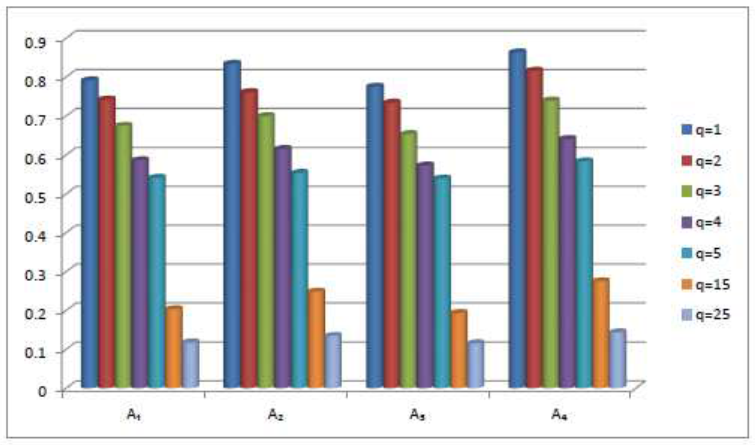
6.1. Sensitivity Analysis

With the flexibility and sensitivity of the parameter q, the suggested CCq-ROFWA operator and CCq-ROFWG operator were used to conducted an analysis to look at the variation in the scores and ranks of alternatives. The relevant findings are summarized in

Table 7. Ranking order of the alternatives using CCq-ROFWA operator and different values of the perimeter q.

q	Score Values				Ranking
	${\mathit{A}}_{\mathbf{1}}$	${\mathit{A}}_{\mathbf{2}}$	${\mathit{A}}_{\mathbf{3}}$	${\mathit{A}}_{\mathbf{4}}$
$q=1$	$0.791$	$0.838$	$0.775$	$0.863$	$A_4>A_2>A_1>A_3$
$q=2$	$0.742$	$0.761$	$0.734$	$0.816$	$A_4>A_2>A_1>A_3$
$q=3$	$0.674$	$0.699$	$0.653$	$0.739$	$A_4>A_2>A_1>A_3$
$q=4$	$0.586$	$0.615$	$0.572$	$0.640$	$A_4>A_2>A_1>A_3$
$q=5$	$0.541$	$0.553$	$0.539$	$0.583$	$A_4>A_2>A_1>A_3$
$q=15$	$0.203$	$0.248$	$0.193$	$0.275$	$A_4>A_2>A_2>A_3$
$q=25$	$0.117$	$0.134$	$0.115$	$0.143$	$A_4>A_2>A_1>A_3$

and

Table 8. Ranking of the alternatives using CCq-ROFWG operator for different values of perimeter q.

q	Score Values				Ranking
	${\mathit{A}}_{\mathbf{1}}$	${\mathit{A}}_{\mathbf{2}}$	${\mathit{A}}_{\mathbf{3}}$	${\mathit{A}}_{\mathbf{4}}$
$q=1$	$0.737$	$0.768$	$0.726$	$0.793$	$A_4>A_2>A_1>A_3$
$q=2$	$0.708$	$0.712$	$0.684$	$0.750$	$A_4>A_2>A_1>A_3$
$q=3$	$0.641$	$0.686$	$0.627$	$0.716$	$A_4>A_2>A_1>A_3$
$q=4$	$0.616$	$0.632$	$0.514$	$0.679$	$A_4>A_2>A_1>A_3$
$q=5$	$0.560$	$0.591$	$0.522$	$0.623$	$A_4>A_2>A_1>A_3$
$q=15$	$0.211$	$0.225$	$0.208$	$0.242$	$A_4>A_2>A_2>A_3$
$q=25$	$0.097$	$0.101$	$0.072$	$0.118$	$A_4>A_2>A_1>A_3$

. These two tables make it abundantly evident that distinct score values are discovered for the CCq-ROFWA and CCq-ROFWA operators that correspond to various values of the parameter $q.$ The rankings of the mentioned options that correspond to the various q values taken into account were unaffected by these variations in the score values. Additionally, the score value of the alternatives are relatively high when q is relatively small, that is, between 1 and $25,$ and the scores decrease as q increases. Decision-makers therefore adopt a more optimistic stance when q is between 1 and 25, and when q is large, the pessimistic character of experts is evident. In general, experts may set q’s value differently depending on their needs.

As a result, $A_4$ is the best option; it is the best alternative.

6.2. Validity Test

Uncertain outcomes are a result of the fact that, when applied to the same DM problem, several MCGDM methods provide a different assessment (ranking), in order to assess the validity and reliability of the MCGDM method. In Figure 1, we show the ranking of the alternatives graphically.

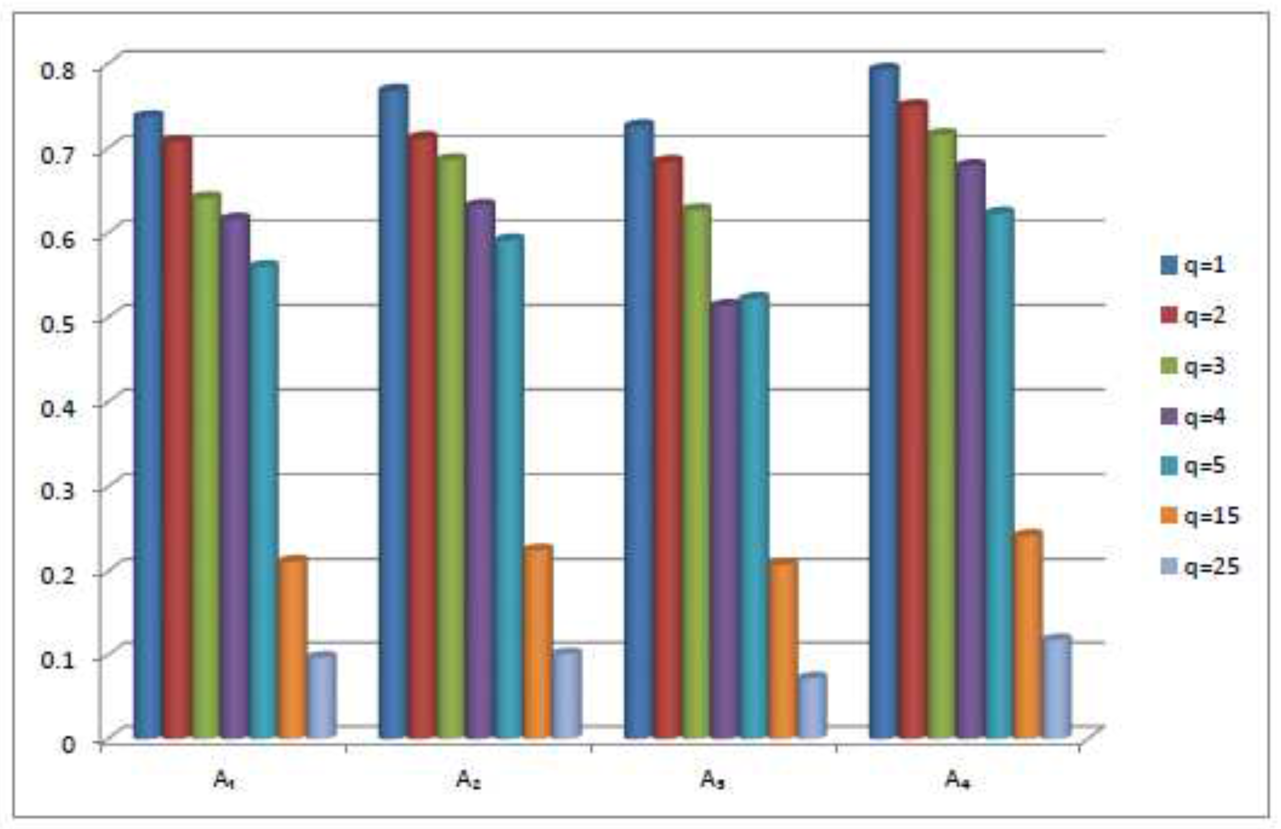
In Figure 2, we show the ranking of the alternatives graphically.

Test criteria 1: The MCGDM method works well when the best alternative is kept as the default and the non-optimal alternative is changed to a worse alternative without altering the relative importance of any decision attribute.

Test criteria 2: Transitive qualities should be followed by an effective MCGDM strategy.

Test criteria 3: When the MCGDM problem is divided into smaller problems and these smaller problems are subjected to the proposed MCGDM approach for the ranking of alternatives, the MCGDM approach is effective. The cumulative rating of the options maintains consistency with the ranking of the original problem.

The following criteria were used to evaluate the obtained solution’s validity.

6.3. Validity Check with Criteria 1

In order to assess the viability of the established technique using criteria 1, the worst alternative $A_4^{/}$ is substituted for the non-optimal alternative $A_4^{/}$ for each expert in the original decision matrix, and the rating values are provided in

Table 9. Transferred alternative $A_4^{/}$ by each expert.

	$C_1$	$C_2$
$E^1$	$〈\left(0.4,2\pi \left(0.4\right)\right),\left(0.3,2\pi \left(0.2\right)\right),0.47〉$	$〈\left(0.5,2\pi \left(0.3\right)\right),\left(0.6,2\pi \left(0.7\right)\right),0.74〉$
$E^2$	$〈\left(0.6,2\pi \left(0.5\right)\right),\left(0.4,2\pi \left(0.7\right)\right),0.92〉$	$〈\left(0.6,2\pi \left(0.8\right)\right),\left(0.4,2\pi \left(0.5\right)\right),0.81〉$
$E^3$	$〈\left(0.5,2\pi \left(0.3\right)\right),\left(0.6,2\pi \left(0.8\right)\right),0.82〉$	$〈\left(0.8,2\pi \left(0.7\right)\right),\left(0.5,2\pi \left(0.4\right)\right),0.95〉$
	$C_3$	$C_4$
$E^1$	$〈\left(0.6,2\pi \left(0.4\right)\right),\left(0.6,2\pi \left(0.7\right)\right),0.83〉$	$〈\left(0.5,2\pi \left(0.4\right)\right),\left(0.6,2\pi \left(0.5\right)\right),0.63〉$
$E^2$	$〈\left(0.4,2\pi \left(0.8\right)\right),\left(0.4,2\pi \left(0.5\right)\right),0.71〉$	$〈\left(0.6,2\pi \left(0.5\right)\right),\left(0.5,2\pi \left(0.6\right)\right),0.75〉$
$E^3$	$〈\left(0.7,2\pi \left(0.5\right)\right),\left(0.7,2\pi \left(0.3\right)\right),0.87〉$	$〈\left(0.7,2\pi \left(0.6\right)\right),\left(0.8,2\pi \left(0.4\right)\right),0.97〉$

.

Utilizing the CCq-ROFOWA operator in step 2 and the Cq-ROFWA operator in step 3 on transferring alternative, we obtain the score values of the alternatives, such as $Sc{o}^{*}\left(A_1\right)=0.454,$$Sc{o}^{*}\left(A_2\right)=0.561,$ $Sc{o}^{*}\left(A_3\right)=0.363,$$Sc{o}^{*}\left(A_4\right)=0.645$. As a result, $A_4$ is ranked as the best alternative in the final ranking of the options, and the proposed method meets test criterion 1.

6.4. Validity Check with Criteria 2 and 3

We split the initial DM problem into smaller decision making problems $\left(A_1,A_2,A_3\right),$$\left(A_2,A_3,A_4\right)$ and $\left(A_1,A_3,A_4\right)$ using these possibilities in order to test the developed MCGDM method using the criteria 2 and 3. When we use the provided MCGDM approach to solve these subproblems, the rating of the alternatives will be as $A_2>A_1>A_3,A_4>A_2>A_3$ and $A_4>A_1>A_3$. We achieve the ultimate ranking order as $A_4>A_2>A_1>A_3$ by adding a ranking of alternatives to the smaller problems. This shows a transitive property and is equivalent to a non-decomposed problem. As a result, the criteria 2 and criteria 3 have same best alternative as the defined MCGDM approach. In

Table 10. Existing methods and their ranking.

Approach	Score Values				Ranking
	${\mathit{A}}_{\mathbf{1}}$	${\mathit{A}}_{\mathbf{2}}$	${\mathit{A}}_{\mathbf{3}}$	${\mathit{A}}_{\mathbf{4}}$
Liu, P. and Liu, J [14]	$0.825$	$0.781$	$0.736$	$0.869$	$A_4>A_1>A_2>A_3$
Liu et al. [23]	$0.585$	$0.557$	$0.595$	$0.664$	$A_4>A_3>A_1>A_2$
Ullah et al. [46]	$0.463$	$0.474$	$0.418$	$0.517$	$A_4>A_2>A_1>A_3$
Garg et al. [47]	$0.175$	$0.221$	$0.192$	$0.268$	$A_4>A_2>A_3>A_1$
Liu et al. [48]	$0.391$	$0.427$	$0.372$	$0.461$	$A_4>A_2>A_1>A_3$

, we show different method their score values and ranking.

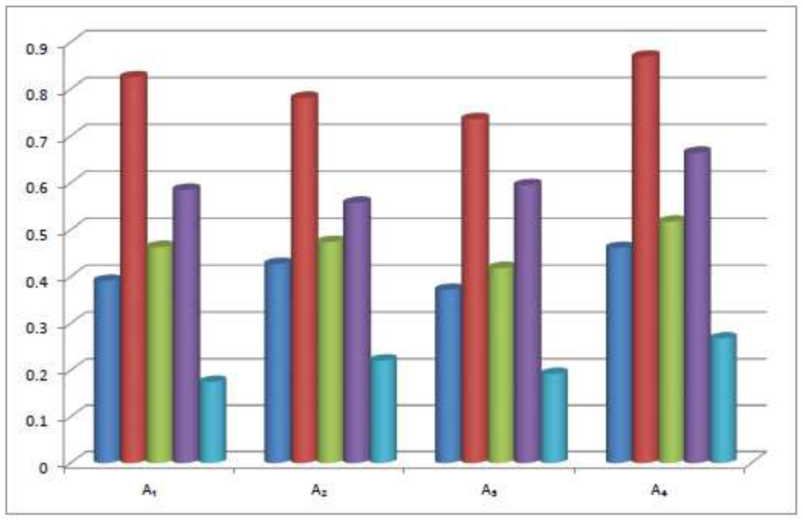
6.5. Comparative Analysis

This section compares the output of the specified MCGDM method with a few of the existing approaches, such as CPFS and Cq-ROFS. To perform this, first the experts’ priorities are converted into CPFS and Cq-ROFS by setting the phase terms to zero. We utilized the available techniques based on this setting; the outcomes are as follows:

In Figure 3, we show the ranking of the alternatives graphically.

7. Conclusions

In this work, an effort has been made to propose different types of aggregation operators regarding the Cq-ROFSs to assist in decision-making. The range of positive degree and negative degree is extended from the real number to the complex number with the unit disc in a variety of current aggregation operators that have previously been proposed to Cq-ROFSs. The defined CCq-ROF aggregation operators are based on the assumption that the experts are unquestionably knowledgeable about object evaluation, i.e., that all experts are given the same amount of confidence to evaluate the various alternatives. Such a circumstance has partially been realized in the simulation of real-world issues. A number of confidence level averaging and confidence levels geometric aggregation operators are proposed in this paper. We describe certain features of these operators while keeping in mind these considerations and the specifics of the Cq-ROFSs. These operators are also used in a decision-making algorithm to demonstrate how the stated operators may more effectively explain real-world situations when employing expert confidence levels during evaluation. By contrasting the specified technique with other existing methods, a numerical example of fire extinguisher selection is provided to illustrate the efficacy and use of the defined method.

In the future, we will extend this approach for complex vague soft sets [38], q-ROF power Maclaurin symmetric mean operators [23], linear Diophantine fuzzy sets [49,50,51], spherical Diophantine fuzzy sets [52], Fractional orthotriple fuzzy rough set [53], and similarity measures for FOFSs using cosine and cotangent functions [54].

References

1. Zadeh, L.A. Fuzzy sets. Inf. Control 1965, 8, 338–353. [Google Scholar] [CrossRef] [Green Version]
2. Jin, L.S.; Xu, Y.Q.; Chen, Z.S.; Mesiar, R.; Yager, R.R. Relative Basic Uncertain Information in Preference and Uncertain Involved Information Fusion. Int. J. Comput. Intell. 2022, 15, 1–7. [Google Scholar] [CrossRef]
3. Li, G.; Yager, R.R.; Zhang, X.; Mesiar, R.; Bustince, H.; Jin, L. Comprehensive Rules-Based and Preferences Induced Weights Allocation in Group Decision-Making with BUI. Int. J. Comput. Syst. 2022, 15, 1–8. [Google Scholar] [CrossRef]
4. Atanassov, K.T. Intuitionistic fuzzy sets. Fuzzy Sets Syst. 1986, 20, 87–96. [Google Scholar] [CrossRef]
5. Yager, R.R. Pythagorean fuzzy subsets. In Proceedings of the 2013 Joint IFSA World Congress and NAFIPS Annual Meeting (IFSA/NAFIPS), Edmonton, AB, Canada, 24–28 June 2013; pp. 57–61. [Google Scholar]
6. Yager, R.R.; Abbasov, A.M. Pythagorean membership grades, complex numbers, and decision making. Int. J. Intell. Syst. 2013, 28, 436–452. [Google Scholar] [CrossRef]
7. Asiain, M.J.; Bustince, H.; Mesiar, R.; Kolesarova, A.; Takac, Z. Negations with respect to admissible orders in the interval-valued fuzzy set theory. IEEE Trans. Fuzzy Syst. 2017, 26, 556–568. [Google Scholar] [CrossRef]
8. Li, H. 3D distances of intuitionistic fuzzy sets based on hesitating index. In Proceedings of the 2018 Chinese Control And Decision Conference (CCDC), Shenyang, China, 9–11 June 2018; pp. 2514–2518. [Google Scholar]
9. Peng, X.; Yang, Y. Some results for Pythagorean fuzzy sets. Int. J. Intell. Syst. 2015, 30, 1133–1160. [Google Scholar] [CrossRef]
10. Garg, H. A new generalized Pythagorean fuzzy information aggregation using Einstein operations and its application to decision making. Int. J. Intell. Syst. 2016, 31, 886–920. [Google Scholar] [CrossRef]
11. Wei, G.; Lu, M. Pythagorean Hesitant Fuzzy Hamacher Aggregation Operators in Multiple-Attribute Decision Making. J. Intell. Syst. 2017, 28, 759–776. [Google Scholar] [CrossRef]
12. Yager, R.R. Generalized orthopair fuzzy sets. IEEE Trans. Fuzzy Syst. 2016, 25, 1222–1230. [Google Scholar] [CrossRef]
13. Liu, P.; Wang, P. Some q-rung orthopair fuzzy aggregation operators and their applications to multiple-attribute decision making. Int. J. Intell. Syst. 2018, 33, 259–280. [Google Scholar] [CrossRef]
14. Liu, P.; Liu, J. Some q-rung orthopair fuzzy Bonferroni mean operators and their application to multi-attribute group decision making. Int. J. Intell. Syst. 2018, 33, 315–347. [Google Scholar] [CrossRef]
15. Riaz, M.; Farid, H.M.A.; Karaaslan, F.; Hashmi, M.R. Some q-rung orthopair fuzzy hybrid aggregation operators and TOPSIS method for multi-attribute decision-making. J. Intell. Fuzzy Syst. 2020, 39, 1227–1241. [Google Scholar] [CrossRef]
16. Riaz, M.; Athar Farid, H.M.; Kalsoom, H.; Pamučar, D.; Chu, Y.M. A robust q-rung orthopair fuzzy Einstein prioritized aggregation operators with application towards MCGDM. Symmetry 2020, 12, 1058. [Google Scholar] [CrossRef]
17. Peng, X.; Dai, J.; Garg, H. Exponential operation and aggregation operator for q-rung orthopair fuzzy set and their decision-making method with a new score function. Int. J. Intell. Syst. 2018, 33, 2255–2282. [Google Scholar] [CrossRef]
18. Wei, G.; Gao, H.; Wei, Y. Some q-rung orthopair fuzzy Heronian mean operators in multiple attribute decision making. Int. J. Intell. Syst. 2018, 33, 1426–1458. [Google Scholar] [CrossRef]
19. Liu, P.; Wang, P. Multiple-attribute decision-making based on Archimedean Bonferroni Operators of q-rung orthopair fuzzy numbers. IEEE Trans. Fuzzy Syst. 2018, 27, 834–848. [Google Scholar] [CrossRef]
20. Liu, Z.; Liu, P.; Liang, X. Multiple attribute decision-making method for dealing with heterogeneous relationship among attributes and unknown attribute weight information under q-rung orthopair fuzzy environment. Int. J. Intell. Syst. 2018, 33, 1900–1928. [Google Scholar] [CrossRef]
21. Du, W.S. Minkowski-type distance measures for generalized orthopair fuzzy sets. Int. J. Intell. Syst. 2018, 33, 802–817. [Google Scholar] [CrossRef]
22. Ali, M.I. Another view on q-rung orthopair fuzzy sets. Int. J. Intell. Syst. 2018, 33, 2139–2153. [Google Scholar] [CrossRef]
23. Liu, P.; Chen, S.M.; Wang, P. Multiple-attribute group decision-making based on q-rung orthopair fuzzy power maclaurin symmetric mean operators. IEEE Trans. Syst. Man Cybern. Syst. 2018, 50, 3741–3756. [Google Scholar] [CrossRef]
24. Yager, R.R.; Alajlan, N.; Bazi, Y. Aspects of generalized orthopair fuzzy sets. Int. J. Intell. Syst. 2018, 33, 2154–2174. [Google Scholar] [CrossRef]
25. Buckley, J.J. Fuzzy complex numbers. Fuzzy Sets Syst. 1989, 33, 333–345. [Google Scholar] [CrossRef]
26. Zhang, G.; Dillon, T.S.; Cai, K.Y.; Ma, J.; Lu, J. Operation properties and δ-equalities of complex fuzzy sets. Int. Approx. Reason. 2009, 50, 1227–1249. [Google Scholar] [CrossRef] [Green Version]
27. Nguyen, H.T.; Kandel, A.; Kreinovich, V. Complex fuzzy sets: Towards new foundations. In Proceedings of the Ninth IEEE International Conference on Fuzzy Systems. FUZZ-IEEE, San Antonio, TX, USA, 7–10 May 2000; pp. 1045–1048. [Google Scholar]
28. Ramot, D.; Milo, R.; Friedman, M.; Kandel, A. Complex fuzzy sets. IEEE Trans. Fuzzy Syst. 2002, 10, 171–186. [Google Scholar] [CrossRef]
29. Yazdanbakhsh, O.; Dick, S. Time-series forecasting via complex fuzzy logic. In Frontiers of Higher Order Fuzzy Sets; Springer: New York, NY, USA, 2015; pp. 147–165. [Google Scholar]
30. Bi, L.; Dai, S.; Hu, B. Complex fuzzy geometric aggregation operators. Symmetry 2018, 10, 251. [Google Scholar] [CrossRef] [Green Version]
31. Chen, Z.; Aghakhani, S.; Man, J.; Dick, S. A neurofuzzy architecture employing complex fuzzy sets. IEEE Trans. Fuzzy Syst. 2010, 19, 305–322. [Google Scholar] [CrossRef]
32. Alkouri, A.M.D.J.S.; Salleh, A.R. September. Complex intuitionistic fuzzy sets. AIP Conf. Proc. 2012, 1482, 464–470. [Google Scholar]
33. Ma, J.; Zhang, G.; Lu, J. A method for multiple periodic factor prediction problems using complex fuzzy sets. IEEE Trans. Fuzzy Syst. 2011, 20, 32–45. [Google Scholar]
34. Dick, S.; Yager, R.R.; Yazdanbakhsh, O. On Pythagorean and complex fuzzy set operations. IEEE Trans. Fuzzy Syst. 2015, 24, 1009–1021. [Google Scholar] [CrossRef]
35. Hu, B.; Bi, L.; Dai, S.; Li, S. Distances of complex fuzzy sets and continuity of complex fuzzy operations. J. Intell. Fuzzy Syst. 2018, 35, 2247–2255. [Google Scholar] [CrossRef]
36. Greenfield, S.; Chiclana, F.; Dick, S. Interval-valued complex fuzzy logic. In Proceedings of the 2016 IEEE International Conference on Fuzzy Systems (FUZZ-IEEE), Vancouver, BC, Canada, 24–29 July 2016; pp. 2014–2019. [Google Scholar]
37. Singh, P.K.; Selvachandran, G.; Kumar, C.A. Interval-valued complex fuzzy concept lattice and its granular decomposition. In Recent Developments in Machine Learning and Data Analytics; Springer: Singapore, 2019; pp. 275–283. [Google Scholar]
38. Selvachandran, G.; Garg, H.; Quek, S.G. Vague entropy measure for complex vague soft sets. Entropy 2018, 20, 403. [Google Scholar] [CrossRef] [PubMed]
39. Selvachandran, G.; Garg, H.; Alaroud, M.H.; Salleh, A.R. Similarity measure of complex vague soft sets and its application to pattern recognition. Int. J. Fuzzy Syst. 2018, 20, 1901–1914. [Google Scholar] [CrossRef]
40. Quek, S.G.; Selvachandran, G.; Davvaz, B.; Pal, M. The algebraic structures of complex intuitionistic fuzzy soft sets associated with groups and subgroups. Sci. Iran. 2019, 26, 1898–1912. [Google Scholar] [CrossRef] [Green Version]
41. Feng, L.; Ma, J.; Wang, Y.; Yang, J. Comparison Study on Development Path for Small and Medium-Sized Enterprises e-Commerce Using Complex Fuzzy Sets. 2018, p. 716. Available online: https://ro.uow.edu.au/smartpapers/240/ (accessed on 20 November 2022).
42. Singh, P.K. Complex fuzzy concept lattice. Neural Process. Lett. 2019, 49, 1511–1526. [Google Scholar] [CrossRef]
43. Selvachandran, G.; Singh, P.K. Interval-valued complex fuzzy soft set and its application. Int. J. Uncertain. Quantif. 2018, 8, 101–117. [Google Scholar] [CrossRef]
44. Garg, H.; Rani, D. New generalised Bonferroni mean aggregation operators of complex intuitionistic fuzzy information based on Archimedean t-norm and t-conorm. J. Exp. Theor. Artif. 2020, 32, 81–109. [Google Scholar] [CrossRef]
45. Garg, H.; Rani, D. Robust Averaging-Geometric Aggregation Operators for Complex Intuitionistic Fuzzy Sets and Their Applications to MCDM Process. Arab. J. Sci. Eng. 2020, 45, 2017–2033. [Google Scholar] [CrossRef]
46. Ullah, K.; Mahmood, T.; Ali, Z.; Jan, N. On some distance measures of complex Pythagorean fuzzy sets and their applications in pattern recognition. Complex Intell. Syst. 2020, 6, 15–27. [Google Scholar] [CrossRef] [Green Version]
47. Garg, H.; Gwak, J.; Mahmood, T.; Ali, Z. Power aggregation operators and VIKOR methods for complex q-rung orthopair fuzzy sets and their applications. Mathematics 2020, 8, 538. [Google Scholar] [CrossRef] [Green Version]
48. Liu, P.; Ali, Z.; Mahmood, T. A method to multi-attribute group decision-making problem with complex q-rung orthopair linguistic information based on heronian mean operators. Int. J. Comput. Syst. 2019, 12, 1465–1496. [Google Scholar] [CrossRef] [Green Version]
49. Riaz, M.; Hashmi, M.R. Linear Diophantine fuzzy set and its applications towards multi-attribute decision-making problems. J. Intell. Fuzzy Syst. 2019, 37, 5417–5439. [Google Scholar] [CrossRef]
50. Riaz, M.; Hashmi, M.R.; Kalsoom, H.; Pamucar, D.; Chu, Y.M. Linear Diophantine fuzzy soft rough sets for the selection of sustainable material handling equipment. Symmetry 2020, 12, 1215. [Google Scholar] [CrossRef]
51. Riaz, M.; Farid, H.M.A.; Aslam, M.; Pamucar, D.; Bozanić, D. Novel approach for third-party reverse logistic provider selection process under linear Diophantine fuzzy prioritized aggregation operators. Symmetry 2021, 13, 1152. [Google Scholar] [CrossRef]
52. Hashmi, M.R.; Tehrim, S.T.; Riaz, M.; Pamucar, D.; Cirovic, G. Spherical linear diophantine fuzzy soft rough sets with multi-criteria decision making. Axioms 2021, 10, 185. [Google Scholar] [CrossRef]
53. Qiyas, M.; Naeem, M.; Abdullah, S.; Khan, F.; Khan, N.; Garg, H. Fractional orthotriple fuzzy rough Hamacher aggregation operators and-their application on service quality of wireless network selection. Alex. Eng. J. 2022, 61, 10433–10452. [Google Scholar] [CrossRef]
54. Naeem, M.; Qiyas, M.; Al-Shomrani, M.M.; Abdullah, S. Similarity Measures for Fractional Orthotriple Fuzzy Sets Using Cosine and Cotangent Functions and Their Application in Accident Emergency Response. Mathematics 2020, 8, 1653. [Google Scholar] [CrossRef]
Figure 1. Ranking of alternatives using CCq-ROFWA operator.
Symmetry 14 02638 g001
Figure 2. Ranking of alternatives using CCq-ROFWG operator.
Symmetry 14 02638 g002
Figure 3. Ranking of alternatives using different methods.
Symmetry 14 02638 g003