
Gas Cooled Graphite Moderated and Pressurized Water Reactor the Optimal Choice for Nuclear Power Plants Based on a New Group Decision-Making Technique

 ,
,  and
and
Abstract
:1. Introduction
1.1. Presented Manuscript’s Contribution
- This study introduces a novel skillful hybrid model, named the m-polar fuzzy soft set, and extends it to include pursuing the periodicity seen in real-world situations.
- We have shown how the novel model works effectively as a tool for grading-based parameterized two-dimensional bipolar fuzzy information.
- We also provided some fundamental procedures and outcomes for an m-polar fuzzy soft set environment. In addition, we developed three nimble algorithms for selecting the optimal answer to multi-attribute decision-making scenarios. The rigorous evaluation of a real-world application also supports the methods.
- This innovative model has the parametric properties of a flexible soft set as well as the distinctive properties of an m-polar fuzzy soft set to handle the double-sided periodic ambiguous data. Table 1 lists the technical specifications as well as the key financial and safety features of each type of thermal reactor (adapted from [14]).
1.2. Overview of the Manuscript Presented
- To identify the best nuclear power facilities, we used models and algorithms.
- To deal with circumstances involving collective decision making where the qualities are interrelated, we presented a family of MAGDM and linear programming to assess objects where the linkages between the attributes are occasionally present.
- A method for multi-attribute group decision making (MAGDM) was devised that is based on an m-bipolar fuzzy set.
- The m-bipolar fuzzy set is given some formal definitions, examples, and qualities that are deduced.
- A new MAGDM method for estimating nuclear power reactors is provided that is based on an m-bipolar fuzzy set.
2. Materials and Methods
3. A Summary of Basic Thermal Reactor Types
Algorithm for Decision Making for the Best Possible Option for Nuclear Power Plants by -Polar Fuzzy Soft Set
| Algorithm 1: Using a 3-polar Fuzzy soft set. |
| Step 1. Provide . |
| Step 2. Calculate where is the -the projection (1,2,3). |
| Step 3. Calculate . |
| Step 4. Put a reasonable weight vector and calculate the score for each . |
| Step 5. The optimum option for the suitability of nuclear power plants based on a 3-polar fuzzy soft set is stated by at its maximum value. |
4. The Finest Nuclear Power Plant Selection Takes into Account the Key Alternative Factors and Has a Greater Impact Thanks to a 2-Polar Fuzzy Soft Set
| Algorithm 2: Using 2-polar Fuzzy soft set. |
| Step 1. Input the possibility m-polar fuzzy soft set defined by two experts |
| Step 2. Compute the 2-polar fuzzy set defined by |
| where is the -the projection ( 1,2); |
| Step 3. Calculate the choice value of by constructing the table |
| and compute |
| Step 4. The maximal value of the score The nuclear power plant’s maximum score and condition are based on a 2-polar fuzzy soft set. |
Suitability of Nuclear Power Plants Based on Two Operations ( and ) of 2-Polar Fuzzy Soft Sets
| Algorithm 3: Using 3-polar Fuzzy soft set. |
| Step 1. State |
| Step 2. Compute |
| Step 3. Compute the 3-polar Fuzzy soft set defined by |
| where is the -the projection |
| Step 4. by where |
| Step 5. The maximal value of to state nuclear power plants based on a 2-polar fuzzy soft set X Based on a 3-polar Fuzzy soft set. |
| Algorithm 4: Using 3-polar fuzzy soft set. |
| Step 1. Compute |
| Step 2. Compute |
| Step 3. Compute the 3-polar fuzzy soft set defined by |
| where is the -the projection |
| Step 4. where |
| Step 5. Compute and compute |
| Step 6. The maximal value of to state the optimal alternative for the suitability of nuclear power plants based on a 2-polar fuzzy soft set X based on a 3-polar fuzzy soft set. Of nuclear power plants based on 2-polar fuzzy soft set X based on 3-polar fuzzy soft set. |
| The second way, compute and compute then, use Table 10 and follow Table 10 to compute Table 10: Compute |
| Algorithm 5: Using 3-polar fuzzy soft set. |
| Step 1. State |
| Step 2. Compute |
| Step 3. Compute the 3-polar fuzzy soft set defined by |
| where is the -the projection |
| Step 4. by where |
| Step 5. The maximal value of to state optimal alternative for suitability of nuclear power plants based on 2-polar fuzzy soft set X based on 3-polar fuzzy soft set. |
| Algorithm 6: Using 3-polar fuzzy soft set. |
| Step 1. State |
| Step 2. Compute |
| Step 3. Compute the 3-polar fuzzy soft set defined by |
| where is the -the projection |
| Step 4. Compute and compute |
| Step 5. The maximal value of to state the optimal alternative for suitability of nuclear power plants based on 2-polar fuzzy soft set X based on 3-polar fuzzy soft set. |
5. Conclusions and Future Directions
5.1. Limitations
5.2. Future Targets
- We can use the suggested approach to solve significant MAGDM issues that arise in real-world settings, such as those related to water waste management, forest management, medical sciences, and other issues.
- Additionally, the work may be expanded to include the most comprehensive complex T-spherical fuzzy N-soft environment. Additionally, because of the adaptability of the innovative m-polar fuzzy soft set model concept, we can also introduce the group decision-supporting scheme.
- Based on the m-polar fuzzy soft set, we have arrived at a criterion for the best choice for the suitability of nuclear power plants.
- In the literature already in existence, a novel design and model of real-life applications have been developed and presented, pointing the way to the best alternative for the applicability of nuclear power plants.
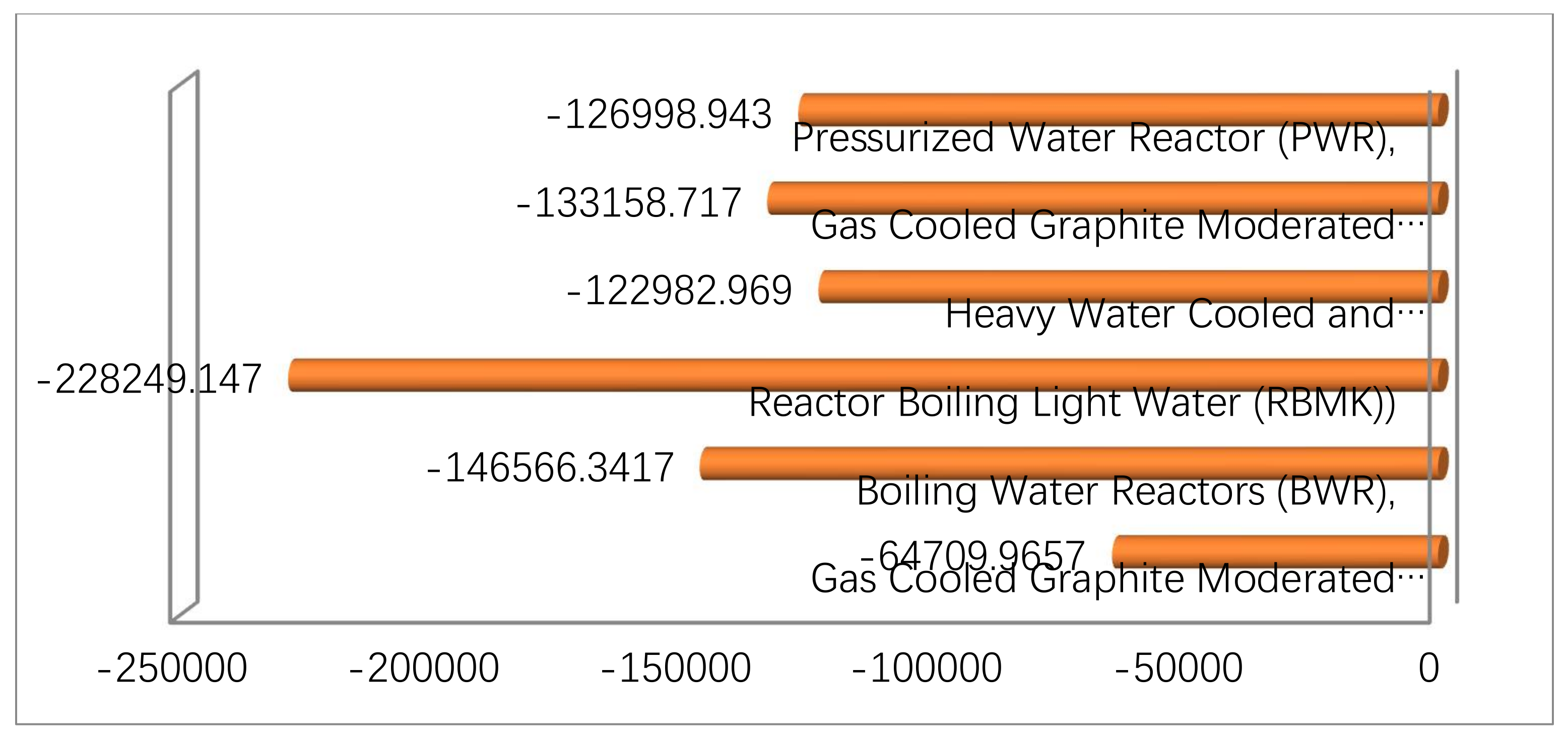
- After analyzing the data, we decided on the following nuclear power plants: Heavy Water Cooled and Moderated, Gas Cooled Graphite-Moderated, Pressurized Water Reactors, Boiling Water Reactors, and Boiling Light Water.
- The algorithms for the analyses’ results have also been noted, and the best option for applications in nuclear power plants is chosen using an m-polar fuzzy soft set decision-making criterion. In the future, we shall apply more advanced theories to Pythagorean fuzzy set decision making based on a Pythagorean fuzzy set.
Author Contributions
Funding
Acknowledgments
Conflicts of Interest
References
- Zadeh, L.A. Fuzzy sets. Inf. Control. 1965, 8, 338–353. [Google Scholar] [CrossRef] [Green Version]
- Akram, M.; Ali, G.; Arif, M.; Alcantud, J.C.R. Novel MCGDM analysis under m-polar fuzzy soft expert sets. Neural Comput. Appl. 2021, 33, 12051–12071. [Google Scholar] [CrossRef]
- Molodtsov, D.A. Soft set theory-first results. Comput. Math. Appl. 1999, 37, 19–31. [Google Scholar] [CrossRef] [Green Version]
- Ali, G.; Akram, M.; Alcantud, J.C.R. Attributes reductions of bipolar fuzzy relation decision systems. Neural Comput. Appl. 2020, 32, 10051–10071. [Google Scholar] [CrossRef]
- Maji, P.K.; Roy, A.R.; Biswas, R. An application of soft sets in a decision making problem. Comput. Math. Appl. 2002, 44, 1077–1083. [Google Scholar] [CrossRef] [Green Version]
- Maji, P.K.; Roy, A.R.; Biswas, R. Fuzzy soft sets. J. Fuzzy Math. 2001, 9, 589–602. [Google Scholar]
- Arooj Adeel, M.A.; Koam, A.N.A. Group Decision-Making Based on m-Polar Fuzzy Linguistic TOPSIS Method. Symmetry 2019, 11, 735. [Google Scholar] [CrossRef] [Green Version]
- Akram, M.; Ali, G.; Alshehr, N.O. A new multi-attribute decision-making method based on m-polar fuzzy soft rough sets. Symmetry 2017, 9, 271. [Google Scholar] [CrossRef] [Green Version]
- Karaaslan, K.; Karatas, S. A new approach to bipolar soft sets and its applications. Discret. Math. Algorithms Appl. 2015, 7, 1550054. [Google Scholar] [CrossRef] [Green Version]
- Akram, M.; Ali, G.; Alcantud, J.C.R. Attributes reduction algorithms for m-polar fuzzy relation decision systems. Int. J. Approx. Reason. 2022, 140, 232–254. [Google Scholar] [CrossRef]
- Waseem, N.; Akram, M.; Alcantud, J.C.R. Multi-Attribute Decision-Making Based on m-Polar Fuzzy Hamacher Aggregation Operators. Symmetry 2019, 11, 1498. [Google Scholar] [CrossRef]
- Akram, M.; Shumaiza; Arshad, M. Bipolar fuzzy TOPSIS and bipolar fuzzy ELECTRE-I methods to diagnosis. Comput. Appl. Math. 2020, 39, 7. [Google Scholar] [CrossRef]
- Fatimah, F.; Rosadi, D.; Hakim, R.B.F.; Alcantud, J.C.R. N-soft sets and their decision making algorithms. Soft Comput. 2018, 22, 3829–3842. [Google Scholar] [CrossRef]
- Nuclear Power in the UK, 1993–1994; Institution of Engineering and Technology: London, UK, 1993; ISBN 0-85296-581-8.
- Wang, H.; Smarandache, F.; Zhang, Y.; Sunderraman, R. Single valued neutrosophic sets. Tech. Sci. Appl. Math. 2010, 17, 10–14. [Google Scholar]
- Zhang, W.R. Bipolar fuzzy sets and relations: A computational framework for cognitive modeling and multiagent decision analysis. In Proceedings of the Industrial Fuzzy Control and Intelligent Systems Conference, and the NASA Joint Technology Workshop on Neural Networks and Fuzzy Logic and Fuzzy Information Processing Society Biannual Conference, San Antonio, TX, USA, 18–21 December 1994; pp. 305–309. [Google Scholar]
- Akram, M. Bipolar fuzzy graphs. Inf. Sci. 2011, 181, 5548–5564. [Google Scholar] [CrossRef]
- Yang, H.-L.; Li, S.-G.; Yang, W.-H.; Lu, Y. Notes on “bipolar fuzzy graphs”. Inf. Sci. 2013, 242, 113–121. [Google Scholar] [CrossRef]
- Chen, J.; Li, S.-G.; Ma, S.-Q.; Wang, X. m-Polar fuzzy sets: An extension of bipolar fuzzy sets. Sci. World J. 2014, 2014, 416530. [Google Scholar] [CrossRef] [PubMed] [Green Version]
- Koczy, L.T. Vectorial I-fuzzy Sets. In Approximate Reasoning in Decision Analysis; Gupta, M.M., Sanchez, E., Eds.; North Holland: Amsterdam, The Netherlands, 1982; p. 151C156. [Google Scholar]
- Akram, M. Neha Waseemand Peide Liu, Novel Approach in Decision Making with m-Polar Fuzzy ELECTRE-I. Int. J. Fuzzy Syst. 2019, 21, 1117–1129. [Google Scholar] [CrossRef]


| Comparison Approach | Fuel | Moderator | Heat Extraction | Outlet Temp. | Pressure |
|---|---|---|---|---|---|
| Gas Cooled Graphite-Moderated (Magnox) | Natural uranium metal (0.7% U235) Magnesium alloy cladding | Graphite | Fuel heated carbon dioxide gas produces steam in a steam generator | 360 °C | 300 psia |
| Gas Cooled Graphite-Moderated (AGR) | Uranium dioxide enriched to 2.3% U235 Stainless steel cladding | Graphite | Fuel heated carbon dioxide gas creates steam in a steam generator | 650 °C | 600 psia |
| Pressurized Water Reactor (PWR) | Uranium dioxide enriched to 3.2% U235 Zirconium alloy cladding | Light Water | Pumping pressurized light water to a steam generator that generates steam in a different circuit | 317 °C | 2235 psia |
| Boiling Water Reactors (BWR), | Uranium dioxide enriched to 2.4% U235 Zirconium alloy cladding | Light Water | Steam produced when pressurized light water boils in the pressure vessel directly runs a turbine | 286 °C | 1050 psia |
| Heavy Water Cooled and Moderated (CANDU)), | Unenriched uranium dioxide (0.7% U235) Zirconium alloy cladding | Heavy water | A steam generator in a separate circuit generates steam from heavy water that is pumped under pressure over the fuel | 305 °C | 1285 psia |
| Reactor Boiling Light Water (RBMK)) | Uranium dioxide enriched to 1.8% U235 | Graphite | Light water boiled with pressure, steam employed to power a turbine | 284 °C | 1000 psia |
| Comparison approach | Spent Fuel Reprocessing | Steam Cycle Efficiency | Main Economic and Safety Characteristics | ||
| Gas-Cooled Graphite-Moderated (Magnox) | Usually within a year, for practical purposes | 31% | Coolant’s inability to change phases has a safety benefit. Additional potential for high availability comes from the ability to refuel while operating | ||
| Gas-Cooled Graphite-Moderated (AGR) | Can be kept underwater for tens of years, although storage in a dry environment may last longer | 42% | Higher operating temperatures and pressures provide the same operational and safety benefits as Magnox while lowering capital costs and increasing steam cycle efficiencies | ||
| Pressurized Water Reactor (PWR) | Long-term storage underwater allows for flexibility in waste management | 32% | Low manufacturing costs as a result of the design’s suitability for production in factory-built subassemblies. Worldwide, a wealth of operational expertise has been accumulated. Refueling required after offloading | ||
| Boiling Water Reactors (BWR), | Regarding PWR | 32% | Similar PWR construction cost benefits improved by the lack of a heat exchanger are compensated by the need for some steam circuit and turbine shielding. Offload refueling is required | ||
| Heavy Water Cooled and Moderated (CANDU), | Regarding PWR | 30% | Good operational history, but infrastructure is needed to produce large volumes of heavy water at affordable prices | ||
| Reactor Boiling Light Water(RBMK) | Information is unavailable | 31% | Information unavailable, although they were present throughout the old USSR in large numbers. believed to be inherently less safe in the West | ||
| Comparison Approach | Fuel | Moderator | Heat Extension | Outlet Temp. | Pressure | Spent Fuel Reprocessing | Steam Cycle Efficiency | Degree of Economic and Safety Levels |
|---|---|---|---|---|---|---|---|---|
| Magnox | 0.70% | 0.8 | 0.9 | 360 | 300 | 0.5 | 31% | 0.9 |
| AGR | 2.30% | 0.8 | 0.9 | 650 | 600 | 0.8 | 42% | 0.95 |
| PWR | 3.20% | 0.8 | 0.8 | 317 | 2235 | 0.7 | 32% | 0.6 |
| BWR | 2.40% | 0.8 | 0.7 | 286 | 1050 | 0.7 | 32% | 0.65 |
| CANDU | 0.70% | 0.85 | 0.7 | 305 | 1285 | 0.7 | 30% | 0.5 |
| RBMK | 1.80% | 0.8 | 0.6 | 284 | 1000 | N/A | 31% | 0.51 |
| Fuel | Moderator | Heat Extension | Outlet temp. | Pressure | Reprocessing of Spent Fuel | Efficiency of the Steam Cycle | Economic and Safety Levels |
|---|---|---|---|---|---|---|---|
| 3.20% | 0.85 | 0.6 | 650 | 1285 | 0.7 | 32% | 0.65 |
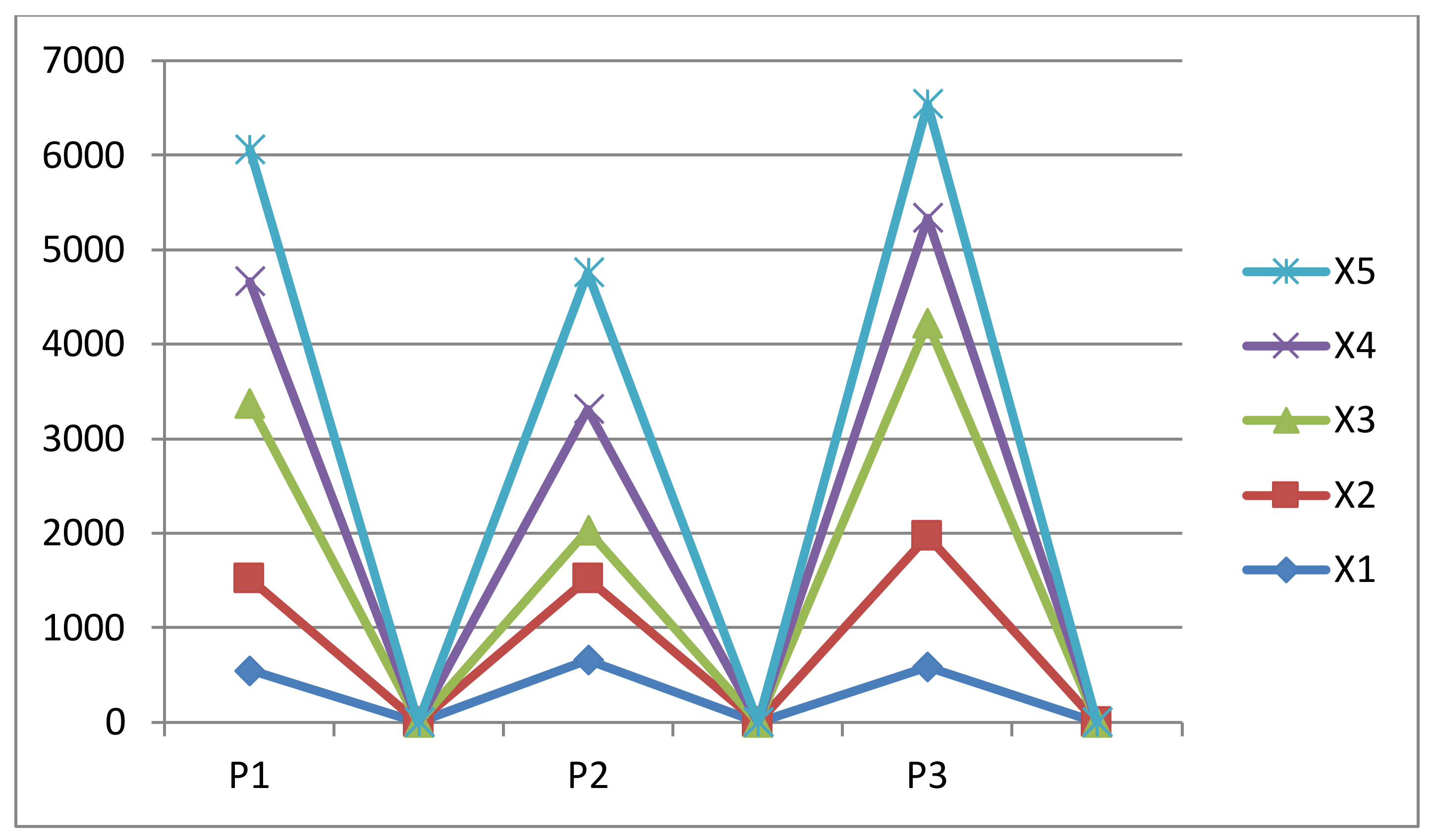
| 553.2773 | 969.4683 | 1854.028 | 1285.091 | 1402.883 | 1105.907 | |
| 660.2693 | 861.231 | 510.3175 | 1278.936 | 1448.67 | 1241.165 | |
| 586.6055 | 1389.235 | 2250 | 1114.787 | 1200.749 | 1156.932 |
| Gas Cooled Graphite-Moderated (Magnox), | Boiling Water Reactors (BWR), | Reactor Boiling Light Water (RBMK)) | Heavy Water Cooled and Moderated (CANDU) | Gas Cooled Graphite-Moderated (AGR), | Pressurized Water Reactor (PWR), |
|---|---|---|---|---|---|
| −64,709.9657 | −146,566.3417 | −228,249.147 | −122,982.969 | −133,158.717 | −126,998.943 |
| Comparison Approach | Fuel | Outlet Temp. | Pressure | Steam Cycle Efficiency |
|---|---|---|---|---|
| Magnox | Natural uranium metal (0.7% U235) Magnesium alloy cladding | 360 °C | 300 psia | 31% |
| AGR | Uranium dioxide enriched to 2.3% U235 Stainless steel cladding | 650 °C | 600 psia | 42% |
| PWR | Uranium dioxide enriched to 3.2% U235 Zirconium alloy cladding | 317 °C | 2235 psia | 32% |
| BWR | Uranium dioxide enriched to 2.4% U235 Zirconium alloy cladding | 286 °C | 1050 psia | 32% |
| CANDU | Unenriched uranium dioxide (0.7% U235) Zirconium alloy cladding | 305 °C | 1285 psia | 30% |
| RBMK | Uranium dioxide enriched to 1.8% U235 | 284 °C | 1000 psia | 31% |
| Magnox | (0.7% U235) | 360 °C | 300 psia | 31% |
| AGR | 2.3% U235 | 650 °C | 600 psia | 42% |
| PWR | 3.2% U235 | 317 °C | 2235 psia | 32% |
| BWR | 2.4% U235 | 286 °C | 1050 psia | 32% |
| CANDU | (0.7% U235) | 305 °C | 1285 psia | 30% |
| RBMK | 1.8% U235 | 284 °C | 1000 psia | 31% |
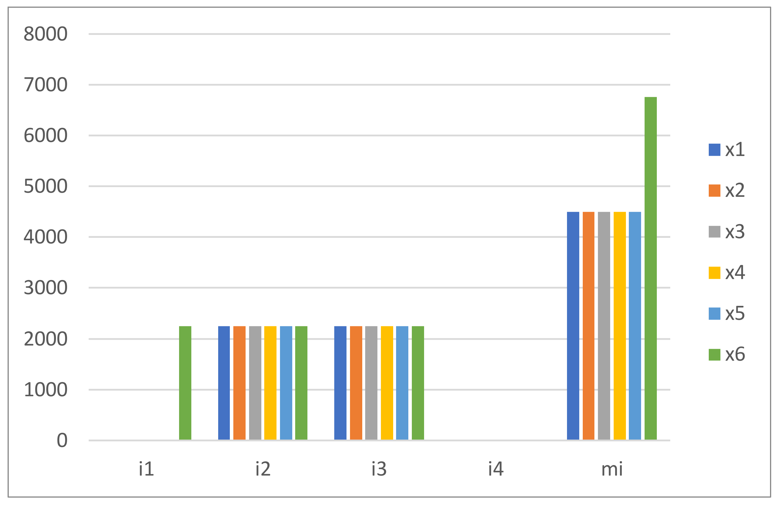
| 0.000821 | 2250 | 2250 | 0.195 | 4500.195821 | |
| 0.000759 | 2250 | 2250 | 0.204 | 4500.204 | |
| 0.000801 | 2250 | 2250 | 0.189 | 4500.189801 | |
| 0.000607 | 2250 | 2250 | 0.195 | 4500.195607 | |
| 0.000747 | 2250 | 2250 | 0.183 | 4500.183747 | |
| 2250 | 2250 | 2250 | 0.153 | 6750.153 |
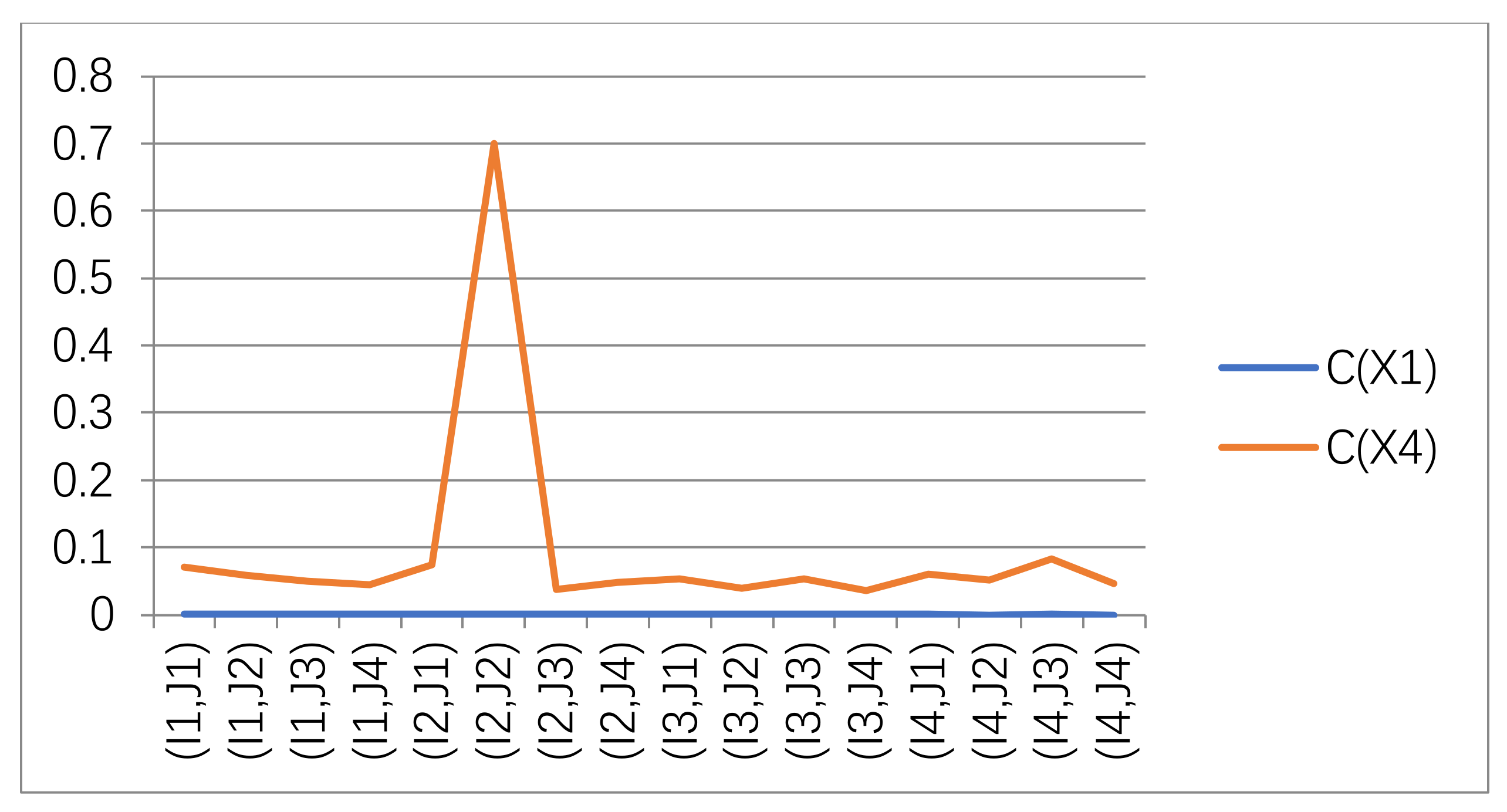
| 0.000011628 | 2250 | 2250 | 0.06975 | |
| 0.000009453 | 2250 | 2250 | 00.0585 | |
| 0.000010680 | 2250 | 2250 | 00.0486 | |
| 0.000009508 | 2250 | 2250 | 00.0441 | |
| 0.000010640 | 2250 | 2250 | 0.07356 | |
| 0.000008896 | 2250 | 2250 | 000.7011 | |
| 0.000010560 | 2250 | 2250 | 0.037908 | |
| 0.000010880 | 2250 | 2250 | 0.0477 | |
| 00.00001064 | 2250 | 2250 | 0.05304 | |
| 0.000009408 | 2250 | 2250 | 0.039 | |
| 00.00001096 | 2250 | 2250 | 0.0522 | |
| 0.000009508 | 2250 | 2250 | 0.0357 | |
| 0.000007412 | 2250 | 2250 | 0.06015 | |
| 0.000004796 | 2250 | 2250 | 0.05205 | |
| 0.00000876 | 2250 | 2250 | 0.08316 | |
| 0.000088592 | 2250 | 2250 | 0.0459 |
| 0.000011628 | 2250 | 2250 | 0.06975 | |
| 0.000009453 | 2250 | 2250 | 00.0585 | |
| 00.00001068 | 2250 | 2250 | 00.0486 | |
| 0.000009508 | 2250 | 2250 | 00.0441 | |
| 0.000010640 | 2250 | 2250 | 0.07356 | |
| 0.000008896 | 2250 | 2250 | 000.7011 | |
| 0.000010560 | 2250 | 2250 | 0.037908 | |
| 0.000010880 | 2250 | 2250 | 0.0477 | |
| 00.00001064 | 2250 | 2250 | 0.05304 | |
| 0.000009408 | 2250 | 2250 | 0.039 | |
| 00.00001096 | 2250 | 2250 | 0.0522 | |
| 0.000009508 | 2250 | 2250 | 0.0357 | |
| 0.000007412 | 2250 | 2250 | 0.06015 | |
| 0.000004796 | 2250 | 2250 | 0.05205 | |
| 0.00000876 | 2250 | 2250 | 0.08316 | |
| 0.000088592 | 2250 | 2250 | 0.0459 | |
| 0.000232321 | 36,000 | 36,000 | 1.502418 |
| 0.000015158 | 2250 | 2250 | 0.1812 | |
| 0.000021538 | 2250 | 2250 | 0.15383 | |
| 0.000015078 | 2250 | 2250 | 0.07125 | |
| 0.000351168 | 2250 | 2250 | 0.0759 | |
| 0.000013984 | 2250 | 2250 | 1.260 | |
| 0.000013302 | 2250 | 2250 | 0.168 | |
| 0.000313140 | 2250 | 2250 | 0.1108 | |
| 0.000013698 | 2250 | 2250 | 0.12944 | |
| 0.000015538 | 2250 | 2250 | 0.0956 | |
| 0.000014058 | 2250 | 2250 | 0.14825 | |
| 0.000013988 | 2250 | 2250 | 0.06114 | |
| 0.000013698 | 2250 | 2250 | 0.06894 | |
| 0.000015200 | 2250 | 2250 | 0.102 | |
| 0.000013760 | 2250 | 2250 | 0.15655 | |
| 0.000000119 | 2250 | 2250 | 0.0792 | |
| 0.000011250 | 2250 | 2250 | 0.0663 |
| 0.000015158 | 2250 | 2250 | 0.1812 | |
| 0.000021538 | 2250 | 2250 | 0.15383 | |
| 0.000015078 | 2250 | 2250 | 0.07125 | |
| 0.000351168 | 2250 | 2250 | 0.0759 | |
| 0.000013984 | 2250 | 2250 | 1.260 | |
| 0.000013302 | 2250 | 2250 | 0.168 | |
| 0.000313140 | 2250 | 2250 | 0.1108 | |
| 0.000013698 | 2250 | 2250 | 0.12944 | |
| 0.000015538 | 2250 | 2250 | 0.0956 | |
| 0.000014058 | 2250 | 2250 | 0.14825 | |
| 0.000013988 | 2250 | 2250 | 0.06114 | |
| 0.000013698 | 2250 | 2250 | 0.06894 | |
| 0.000015200 | 2250 | 2250 | 0.102 | |
| 0.000013760 | 2250 | 2250 | 0.15655 | |
| 0.000000119 | 2250 | 2250 | 0.0792 | |
| 0.000011250 | 2250 | 2250 | 0.0663 | |
| 0.000854677 | 36,000 | 36,000 | 2.9284 |
Publisher’s Note: MDPI stays neutral with regard to jurisdictional claims in published maps and institutional affiliations. |
© 2022 by the authors. Licensee MDPI, Basel, Switzerland. This article is an open access article distributed under the terms and conditions of the Creative Commons Attribution (CC BY) license (https://creativecommons.org/licenses/by/4.0/).
Share and Cite
Khalaf, M.M.; Ismail, R.; Al-Shamiri, M.M.A.; Abdelwahab, A.M. Gas Cooled Graphite Moderated and Pressurized Water Reactor the Optimal Choice for Nuclear Power Plants Based on a New Group Decision-Making Technique. Symmetry 2022, 14, 2621. https://doi.org/10.3390/sym14122621
Khalaf MM, Ismail R, Al-Shamiri MMA, Abdelwahab AM. Gas Cooled Graphite Moderated and Pressurized Water Reactor the Optimal Choice for Nuclear Power Plants Based on a New Group Decision-Making Technique. Symmetry. 2022; 14(12):2621. https://doi.org/10.3390/sym14122621
Chicago/Turabian StyleKhalaf, Mohammed M., Rashad Ismail, Mohammed M. Ali Al-Shamiri, and Abdelazeem M. Abdelwahab. 2022. "Gas Cooled Graphite Moderated and Pressurized Water Reactor the Optimal Choice for Nuclear Power Plants Based on a New Group Decision-Making Technique" Symmetry 14, no. 12: 2621. https://doi.org/10.3390/sym14122621