Cancer Therapy Assessment Accounting for Heterogeneity Using q-Rung Picture Fuzzy Dynamic Aggregation Approach

Abstract

Due to the fact that there is no symmetry in the division of cancer cells, it is important to consider this asymmetrical behavior. Because of this heterogeneity during any therapy, not every cancer cell that is killed only is abolished, which is sensitive to the particular treatment chosen. Mathematical models that describe these pathways are critical for predicting cancer cell proliferation behavior. The literature on the mathematical modeling of cancer onset, growth, and metastasis is extensive. Both deterministic and stochastic factors were used to develop mathematical models to mimic the development rate of cancer cells. We focus on the cell’s heterogeneity in our model so that the cells generally responsible for spreading cancer, which are called stem cells, can be killed. Aggregation operators (AOs) play an important role in decision making, especially when there are several competing factors. A key issue in the case of uncertain data is to develop appropriate solutions for the aggregation process. We presented two novel Einstein AOs: q-rung picture fuzzy dynamic Einstein weighted averaging (q-RPFDEWA) operator and q-rung picture fuzzy dynamic Einstein weighted geometric (q-RPFDEWG) operator. Several enticing aspects of these AOs are thoroughly discussed. Furthermore, we provide a method for dealing with multi-period decision-making (MPDM) issues by applying optimal solutions. A numerical example is presented to explain how the recommended technique can be used in cancer therapy assessment. Authenticity analysis is also presented to demonstrate the efficacy of the proposed technique. The suggested AOs and decision-making methodologies are generally applicable in real-world multi-stage and dynamic decision analysis.

1. Introduction

Cancer is the second most serious health problem worldwide, currently causing an estimated 9.6 million deaths every year. Cancer took the lives of 9.56 million people in 2017, according to the Global Burden of Disease (GBD). Cancer is also the reason for one in every six deaths. Various kind of cancers including lung, colorectal, stomach, and liver cancers mostly affect men, while breast, colorectal, lung, cervical, and thyroid cancers mostly affect women. In recent years, cancer has become a very frequent disease around the world. It causes significant emotional, physical, and financial strains on individuals and their families, communities, and health systems. Many middle-to-low income countries’ health systems are unable to properly deal with this disease, and cancer patients worldwide lack immediate access to good quality treatment.

In advanced economies, where people are much less likely to succumb to contagious diseases and other fatal conditions causing premature death, cancer is a highly common cause of death. Among all diseases, research on cancer is important as this disease emotionally affects humans and a person can become completely convinced that they definitely will not survive for long. In a general sense, research provides us all with a plethora of data regarding the basic mechanisms involved in the onset, growth, and spread of cancer in the body [1]. To conduct in cancer treatment is important because as mentioned earlier cancer is one of the main cause of deaths in the world. The Figure 1 present that cancer is the second main cause of deaths in the world.

The main purpose of conducting research on cancer treatment is to produce safe and effective strategies for screening, detecting, curing, and, ultimately, cancer-related disorders. These will enable us to control the effects of cancer spread which are costly in terms of precious human life. Due to the fact that cancer is currently a popular research topic, we have gained a lot of understanding about what biological mechanisms are involved in cancer genesis, growth, and spread in the body. As a result of such work, more effective and targeted treatments and prevention strategies have been introduced.

People who are diagnosed with cancer earlier experience more timely and effective care lower healthcare morbidity, and a better quality of life than those who are diagnosed later. Early cancer identification is a complex and multifaceted matter that has dominated global strategy and charity initiatives. Two different patient behaviors can assist in early cancer detection. Attending cancer screenings (e.g., a mammography for breast cancer) and disclosing suspected symptoms to primary care as soon as feasible are two examples.

Such different survival rates push us to make progress in cancer research to control its effects as well as its spread and ultimately remove it from the human body. All forms of control are possible if the cancer has been diagnosed at a very early stage of its spread. The Figure 2 and the Figure 3 display the fact that the survival rate is greater when the cancer in the stomach and pancreas is at a comparatively earlier stage. The early detection and treatment of cancer can be encouraged by activities such as promoting screening, providing education and community outreach activities, aiding patient navigators and health personnel in their efforts to reduce obstacles to cancer information, resources, and treatment, and working within wellness systems to improve service quality.

Literature Review

Human questioning is heavily based on imprecisely defined lessons. Most natural lessons and conceptions are fuzzy as opposed to crisp, which offers upward push to fuzzy set theory. People, on the other hand, can nicely approximate lessons which is sufficient to perform a large variety of activities . Humans can summarize massive quantities of statistics and use these to successfully carry out activities. Because of its tolerance for such imprecision, fuzzy common sense is well suited for complicated systems. The predominant contributions that fuzzy control, estimation, and measuring generation have made in each of the identified problems were identified during the scientific literature search [2].

Colorectal cancer (CRC) is the most common digestive system-associated cancer and has become one of the deadliest illnesses in the world. Given the negative diagnosis of CRC, it is of paramount importance that the prediction and detection of this disease are made more accurate. Early CRC detection using computational technology can notably enhance the general survival probability of patients. As a result, the study in [3] aimed to increase the accuracy of CRC detection methods by a fuzzy common sense-based totally clinical decision assist system (FL-based totally CDSS).

Furthermore, a modified intuitionistic fuzzy clustering method is developed for segmenting a lesion/tumor in mammogram pictures. A singular intuitionistic fuzzy generator is used to compute the non-club degree of the bushy picture and an intuitionistic fuzzy image is created. From an intuitionistic fuzzy club characteristic, two club stages are computed using a fuzzy hedge. These two club levels are combined by the use of Zadeh’s t norm and an interval kind 2 fuzzy image is acquired. The photo is then clustered in different areas where four fuzzy features are used. The styles of distance capabilities—fuzzy divergence and fuzzy exponential kind distance capabilities—are used in the clustering algorithm [4].

Decision making is an important component of daily life, and it is applied in sophisticated and organization-wide decisions. These acts require aggregation processes, which aggregate the many preferences into a general value, taking into consideration all individual aspects. Aggregation is defined as the process of merging numerical values into a single number that represents the collection of numbers. Decision-making problems are prevalent in a variety of fields, including engineering, accounting, and communications. Historically, it has been assumed that all information about accessible alternatives will be presented in the form of quantitative data, because dealing with imprecision and ambiguity in data is crucial in real-world circumstances.

In 1965, Zadeh [5] introduced the concept of fuzzy set (FS) as a strategy for coping with uncertainty. There is a function in FS that returns an object’s degree of membership to a non-empty set from the closed unit interval $[0,1]$. FSs have several uses in business strategy, pattern recognition, and other areas. As an extension of FS theory, Atanassov [6] devised the innovative idea of “intuitionistic fuzzy set” (IFS) theory. It is crucial to understand that FS may be characterized in terms of membership elements, but IFS can be described in terms of both membership and non-membership aspects. While IFS has been widely used to address major difficulties, there are some circumstances under which it cannot be used. Assume that, while voting, the human viewpoint contains more replies than classic FS and IFS can effectively portray, such as yes, abstain, no, and refuse. Cuong pioneered the notion of a “picture fuzzy set” (PFS) to solve these issues [7]. Each element in the set has a “positive membership grade” (PMSG), a “neutral membership grade” (N ${}_u$ MSG), and a “negative membership grade” (N ${}_g$ MSG) with values in the range of $[0,1]$.

Cuong [8] investigated several PFS features and developed a method for measuring the distance between PFSs. Wei et al. offered the “projection model” [9], “generalized dice similarity measurements” [10], and “similarity measures” [11] for PFS. Cuong and Hai [12] established essential logic operators, disjunctions, conjunctions, and negations, as well as the main operations for fuzzy derivation forms for PFSs. Phong et al. [13] looked into a variety of PF-related configurations. Riaz et al. [14] updated numerous basic PFS operations.

Over the last two decades, there has been a lot of emphasis on information fusion and enhanced AOs. The efficiency and limitations of AO have been engrained in decision making. It is evident that AO provides a range of operational rules for merging a finite set of fuzzy numbers into a single fuzzy number. Data aggregation is vital in strategic planning, marketing, finance, medicine, science, and investigations. Many AOs have been developed in terms of functions and operational laws for PFNs. Wang et al. [15] pioneered the use of “Muirhead mean AOs” for PFNs. Garg [16] proposes a significant number of averaging and ordered averaging AOs for PFNs. Tian et al. [17] defined some “picture fuzzy power Choquet-ordered geometric AOs” and “picture fuzzy power Shapley Choquet-ordered geometric AOs” with Shapley fuzzy measure-based multi-criteria decision making (MCDM). Wei [18] pioneered the notion of Hamacher AOs, while Jana et al. [19] suggested Dombi AOs for PFNs. Wang et al. [20] suggested a hotel building energy efficiency rehabilitation project selection under PFSs. Riaz and Farid [21] proposed a hierarchical medical diagnosis approach for COVID-19 with the help of picture-fuzzy fairly AOs. Naeem et al. [22] proposed the Aczel–Alsina picture fuzzy AOs with MCDM. Farid and Riaz [23] proposed some new Einstein interactive geometric AOs for q-rung orthopair fuzzy sets (q-ROFSs). Saha et al. [24] presented novel hybrid hesitant fuzzy weighted AOs for MCDM based on Archimedean and Dombi operations. MCDM employing q-ROF weighted fairly AOs was suggested by Saha et al. [25]. Akram et al. [26] proposed an extension relating to competition graphs. Karaaslan and Ozlu, [27] proposed correlation coefficients for dual type-2 hesitant fuzzy sets. Alcantud [28] provided some information about the relationships between fuzzy soft and soft topologies. Decision making is an effective process to provide the most appropriate solution to real-world decision-making scenarios by considering and merging the opinions of various individuals on the problem [29]. Feng et al. [30] presented several intuitionistic fuzzy soft sets.

In actual life, we may encounter various situations that cannot be solved by PFS, such as when the sum of PMSD, ${\mathrm{N}}_u$MSD, and ${\mathrm{N}}_g$MSD > 1. In such a situation, PFS is unable to produce a suitable outcome. Mahmood et al. [31], Ashraf et al. [32], and Gundogdu and Kahraman [33] proposed the idea of a spherical fuzzy set (SFS) independently in their articles. SFS offers the DM more latitude in dealing with uncertainty in decision-making situations. Parimala et al. [34] introduced the Bellman–Ford algorithm in regard to SFSs. Li et al. [35] proposed a novel concept of a q-rung picture fuzzy set (q-RPFS) as an extension of SFS. Akram et al. [36] proposed some Einstein AOs for q-RPFSs. Pinar and Boran [37] introduced some distance measure for q-RPFSs. He et al. [38] proposed some Dombi Hamy mean AOs for q-RPFSs. Liu et al. [39] proposed Yager AOs for q-RPFSs.

In general, previous works have focused on developing models for collecting SF information across the same time span. However, many complicated decision-making situations need to consider the performances of alternatives over time. Such challenges are referred to as multi-period decision-making (MPDM) problems, since they collect data at discrete time intervals within a period. Numerous scholars have explored the temporal generalized variants (commonly referred to as dynamic) of existing fuzzy AOs and analyzed their effectiveness in the MPDM in recent decades. Kamaci et al. [40] proposed the idea of dynamic AOs for interval-valued picture-hesitant fuzzy information and their applications in MPDM. Yang et al. [41] initiated the concept of dynamic intuitionistic fuzzy normal AOs. Jana et al. [42] introduced the concept of dynamic AOs for complex q-ROFSs. Peng and Wang [43] proposed some dynamic AOs for a hesitant fuzzy set with applications to MPDM. Gumus and Bali [44] proposed the novel idea of Einstein dynamic AOs for IFSs with applications to period-based decision making.

Einstein’s t-norms and t-conorms are excellent choices for establishing the product and sum of q-RPFSs, respectively. The Einstein product and sum, which are described in terms of Einstein t-norms and t-conorms, respectively, provide fluent algebraic product and sum approaches. Additionally, these operations define the intersection and union of q-RPFSs, which is a good approximation of the intersection and union structure of q-RPFSs. Additionally, several MCDM approaches incorporate alternative assessments within that time span. Indeed, the evaluation process should take into consideration not just the present performance of alternatives, but also their historical performance. The optimal selection is contingent upon the alternatives’ previous and current performance in certain MCDM issues.

Riaz and Farid proposed hybrid picture fuzzy aggregation operators with applications [45], Saha et al. introduced some distance measures for a picture fuzzy set [46], and Vojinovic et al. introduced a hybrid technique for decision making [47]. Peng and Yang gave some results related to Phytagorean fuzzy sets [48]. Jana et al. proposed some Dombi aggregation operators for the bipolar fuzzy set [49]. Feng et al. [50], Yager and Abbasov [51], and Yager [52] gave some important results for Pythagorean fuzzy sets and q-rung orthopair fuzzy sets. There are many aggregation operators related to different extensions of fuzzy sets, [52,53,54,55].

The remainder of this paper is organized as follows. Section 2 gives some details related to the heterogeneity of cancer cells. Section 3 presents the mathematical modeling of the proposed method. Section 4 provides the basics of q-RPFSs as well as other important ideas. Section 5 explores some dynamic q-RPF Einstein AOs and their appealing features. In Section 6, we used the presented AOs to construct an MCDM method. Section 7 goes into detail about the case study, including numerical examples and an authenticity test. Section 8 outlines the important findings of the study paper.

2. Heterogeneity of Cancer Cells

The heterogeneity of cancer cells makes developing successful treatment techniques extremely difficult. Different cancer cells have different morphological and phenotypic characteristics. Higher efficacy is expected from refined treatment options that incorporate the knowledge of heterogeneity. Heterogeneity in cancer cells can be caused by a variety of factors. Among them, the tumor micro-environment exerts diverse selective pressures on tumor cells and leads to a wider range of dominant sub-clones in different geographical locations of the tumor. Beyond the variety that can be attributed to clonal evolution or environmental changes, cancer stem cell differentiation (see details in Section 2.1) provides a mechanism for producing phenotypic and functional heterogeneity. However, heterogeneity by itself does not rule out the possibility of a cancer stem cell (CSC) hierarchy, according to [56].

The ability to spread is not the same for all cancer cells. Similarly, not all cancer cells respond to treatment in the same way. Any therapy’s outcome is determined by the cell’s characteristics: chemotherapy is more sensitive to some cells than radiotherapy, and vice versa. These treatments can be used separately or in combination. To improve treatment outcomes, radiation can be given before, during, or after chemotherapy. In general, radiation is a highly effective treatment for a wide range of cancers, allowing for a variety of therapeutic goals to be met. However, despite its efficiency, cancer stem cells (see details in Section 2.1) that are considered elements of heterogeneous tumors are relatively insensitive to radiotherapy. Due of their distinct properties, studies have revealed that these cells may be primarily responsible for cancer spread. The total dose specification is critical in radiation interval applications. In addition, the total dose is fractionated (over time) for a variety of reasons: normal cells have more time to heal, but malignant cells have less time to mend between fractions. This also permits tumor cells that were in a radio-resistant phase of the cell cycle during one treatment to develop into a sensitive phase before the next dose is given [57]. Furthermore, the dose of radiotherapy to be provided is determined by a variety of criteria, including the location, size, and kind of cancer. The treatment plan is created by considering the aforementioned factors. Long therapy programs are sometimes recommended, with daily treatment sessions lasting a certain amount of time. Irradiations are required once or twice a day in some treatment plans. Before planning radiation, the issue of tumor heterogeneity must be addressed. Ignoring this could lead to the development of cancer stem cells. Their radiation sensitivity may cause a delay in cancer elimination.

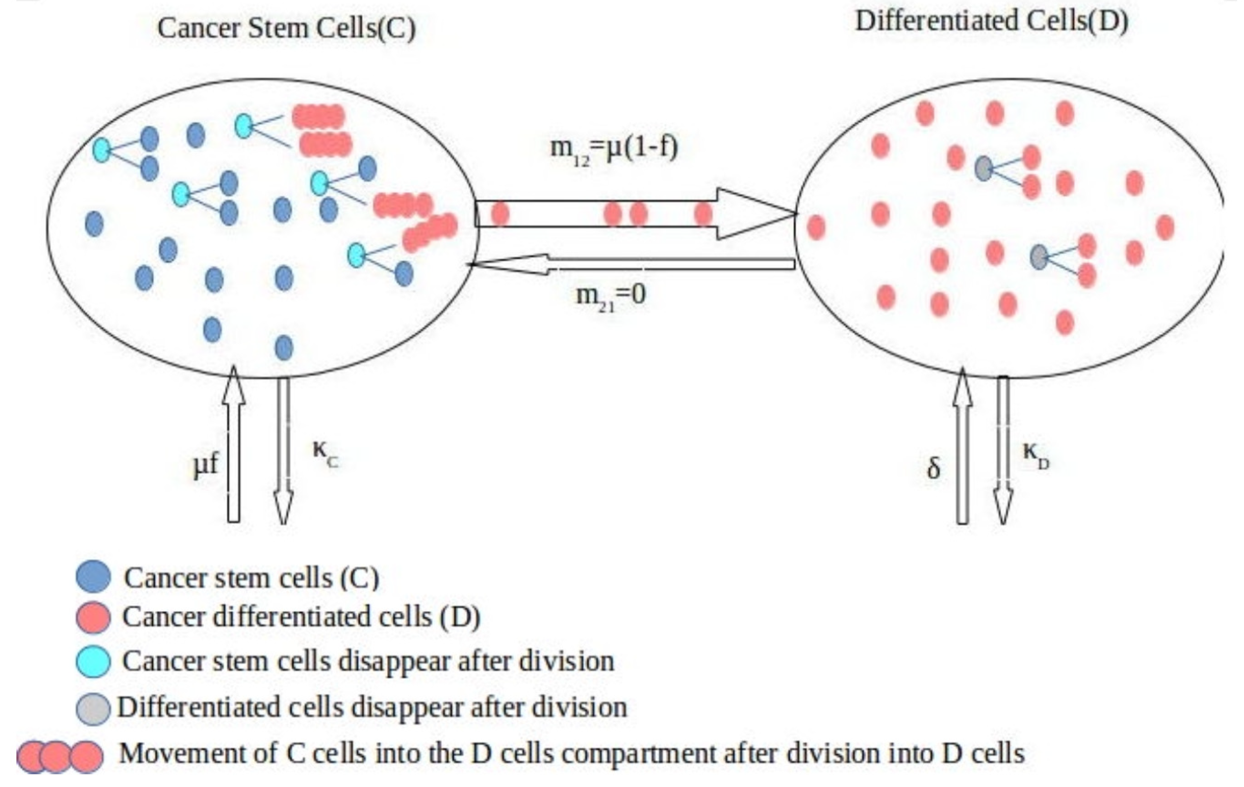
2.1. Theory of Cancer Stem Cells and Differentiated Cancer Cells

Cancer stem cell theory is extremely useful because it elucidates not only the complexity of tumor onset and growth and its capability to metastasize and reoccur, but also the ineffectiveness of traditional cancer remedies. This evaluation examines stem cell residences, inclusive of self-renewal, heterogeneity, and resistance to apoptosis. Because of some similarities between these cells and stem cells (SCs), the former have been named cancer stem cells (CSCs). The CSC model assumes that these cells have the following characteristics: (1) self-renewal; (2) heterogeneity in their capability for multidirectional differentiation; and (3) resistance to apoptosis. It is assumed that these CSC residence decreases the effectiveness of conventional treatment plans that act especially on the differentiated or differentiating tumor cells. The population of undifferentiated CSCs, forming a minor fraction of the tumor mass, is spared [58].

It is thought that a key element regulating the biology of stem cells is their micro-environment cells, such as those of the extracellular matrix, which facilitate self-renewal and survival. As we begin to recognize the pathways that are probably crucial for the CSC environment, we will optimistically be able to correctly goal this cellular population. The precise mobile is related to the identification of CSCs. When inferring a mutation, authentic cells are able to offer upward thrust to a tumor. A cancer stem cell is a self-renewing cell within a tumor that has the capacity to regenerate the phenotypic diversity of the original tumor. Cancer differentiation refers to the degree of development of the cancer cells in a tumor. Well-differentiated tumor cells resemble normal cells and tend to grow and spread at a slower rate than undifferentiated or poorly differentiated tumor cells, which lack the structure and function of normal cells and grow uncontrollably.

2.2. Hypothesis: CSCs Are Responsible for Tumor Growth

There is no symmetry in cancer cell division, which is called asymmetric division. The two most important observations conclude that cancer stem cells are responsible for the growth and persistence of the tumor in the body. Most tumors begin with a single cell, however, not all cells inside a tumor are exactly the same. A tumor, in fact, has many distinct types of cells. Some are cancerous, while others infiltrate normal cells and are thought to guide the growth of cancer cells. Although tumors are produced from a single altered cell, the cells within tumors may exhibit unique phenotypes, reflecting the normal tissue from whence they originate, and have varying proliferation potential. The observed cellular heterogeneity in tumors can be attributed to genetic instability and the selection of cells that can adapt to the tumor micro-environment, providing an affordable explanation for the aforementioned facts. Recent evidence significantly supports the notion that the cancer stem cell model also plays an important role in tumor heterogeneity. Another observation upon which the maximum cancer stem cellular principle is founded was drawn from studies demonstrating that a massive range including most cancer cells had been required to grow a tumor. Tumors have a mobile gradient wherein only a tiny population of tumor stem cells may self-renew and then be transformed into a cell that is definitely capable of successfully regenerating a tumor. Other cancer cells may have a more limited ability to replicate, and as a result, they contribute to the tumor bulk but not to tumor safety [59].

Now, to move towards our treatment strategy, first we will explain the definition of mathematical modeling which is based on the idea of converting real-world problems into mathematical equations.

3. Mathematical Modeling

Mathematical modeling is the technique in which numerous mathematical structures—graphs, equations, diagrams, scatter plots, tree diagrams, and so on—are used to represent real global situations. This offers an abstraction that reduces a problem to its important traits. The flow chart below shows the typical mathematical modeling process [60]. Firstly, the abstract real-world problem is converted into to a well-defined mathematical problem. After making some assumption and introducing some parameters, the mathematical equations that describe the real-world dynamics of the problem are constructed. Subsequently, the mathematical solution or construction numerical simulation solution behavior of the real-world problem is found at the end of the validation by comparing the solution behavior of the mathematical model with the  observed real-world solution. There are many different methods that can model the spread of cancer. Here, our main focus is to propose a treatment strategy which can more effectively kill cancer cells.

3.1. Mathematical Modeling Using Stochastic Differential Equations

In this section, we will construct mathematical models for the interaction between cancer stem cells (C) and differentiated cancer cells (D) in the framework of stochastic differential equations (SDEs). We will consider the three following modeling approaches:

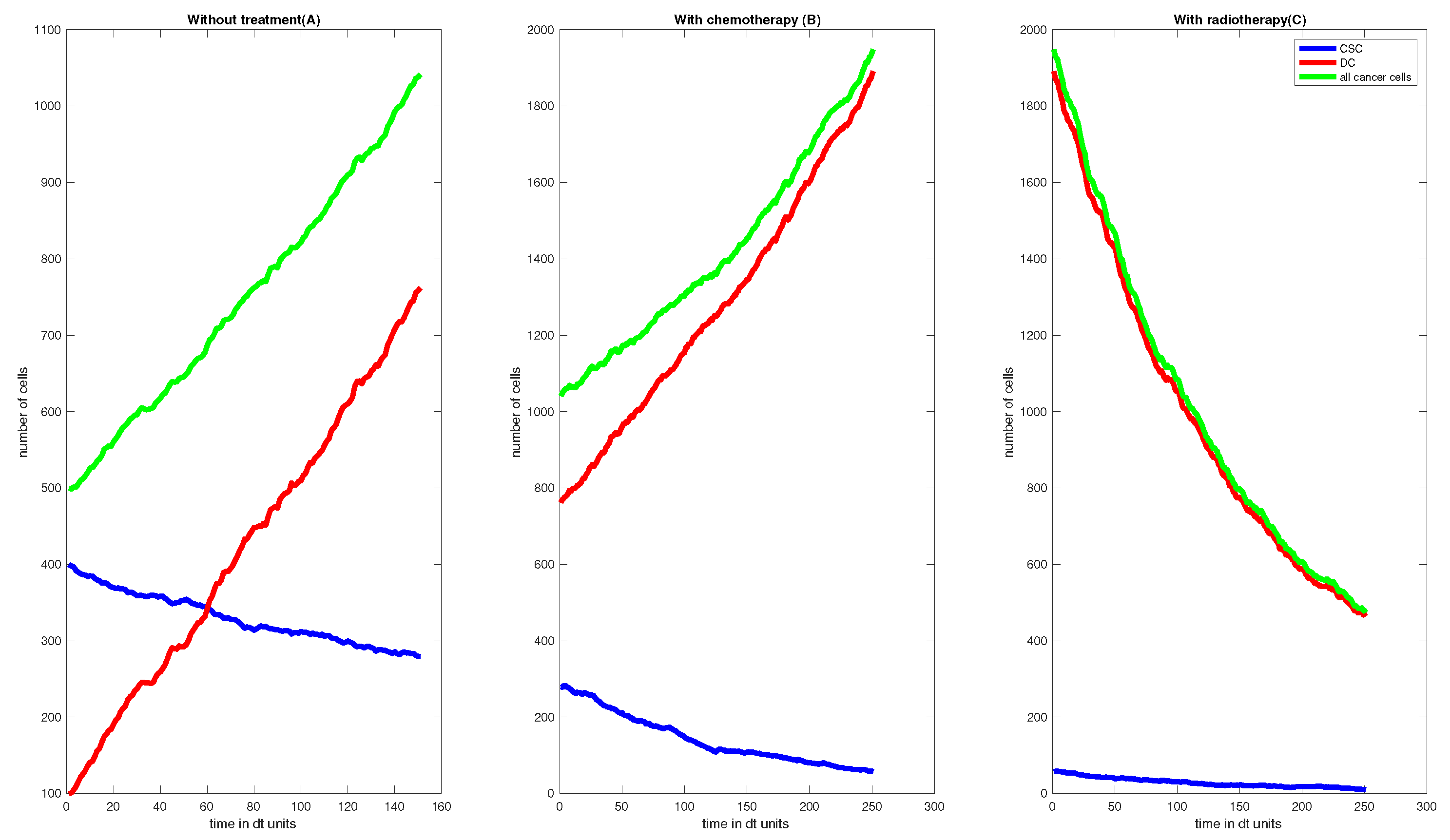
• An SDE model without treatment.
• An SDE model with chemotherapy.
• An SDDE model with chemotherapy and radiotherapy with delay.

An SDE Model for Interaction between Cancer Stem Cells (C) and Differentiated Cells (D)

Let $C\left(t\right)$, $D\left(t\right)$ be the populations of cancer stem cells (C) and differentiated cells (D) at time t, respectively. Let $\mu$$>0$ be the division rate of cancer stem cells (C) and f denote the fraction of CSCs dividing again into two CSCs, where $0<f<1$. The dynamics of C and D can be those of a system of ordinary differential equations (ODEs) using a birth and death model [61]:

$$\begin{array}{c}\hfill \begin{array}{cc}\hfill \frac{dC}{dt}& =2\mu fC-\mu C-{\kappa }_{C}C,\hfill \\ \hfill \frac{dD}{dt}& =2\mu (1-f)C+\delta D-{\kappa }_{D}D.\hfill \end{array}\end{array}$$

(1)

The Figure 4 shows a compartmental analysis of all possible divisions of CSCs (C) and DCs (D). Here, 2$\mu f$ is the fraction of C cells after the division that remained in the compartment of C cells, and 2 $\mu (1-f)$ is the fraction of D cells after the division that went into the compartment of D cells.

We assume here that $\delta <{\kappa }_D$. Let $\delta$ ($\delta \ll 1$) denotes the birth rate of D cells. Assume that ${\kappa }_C$ and ${\kappa }_D$ denote the generic death rates of the C and D cells, respectively.

We deduce an SDE model that shows the interaction between C and D cells. For every change, corresponding probabilities are given in

Table 1. Table of probabilities corresponding to each change.

$\mathit{X}={(\mathit{C},\mathit{D})}^{\mathit{T}}$	Corresponding Probability of Each Change (${\mathit{P}}_{\mathit{i}}$)
$\Delta X_1={(-1,2)}^t$	$P_1=\mu (1-f)C▵t$
$\Delta X_2={(-1,0)}^t$	$P_2={\kappa }_{C}C▵t$
$\Delta X_3={(1,0)}^t$	$P_3=\mu fC▵t$
$\Delta X_4={(0,-1)}^t$	$P_4={\kappa }_{D}D▵t$
$\Delta X_5={(0,1)}^t$	$P_5=\delta D▵t$, $\delta \ll 1$
$\Delta X_6={(1,-1)}^t$	$P_6=m_{21}=0$
$\Delta X_7={(0,0)}^t$	$P_7=1-{\displaystyle \sum _{i=1}^6}{P}_i$ (all other cases)

. We assumed that C cells are either divided into two new C cells or two new D cells. The asymmetric division of C cells into one C cell and one D cell is not considered, as it does not affect the model [62]. Here, $m_{21}=0$ expresses the fact that D cells cannot move into the compartment of C cells.

Equation (1) represents the conversion of observed heterogeneity and the spread of cancer cells in a real problem into stochastic differential equations according to the probabilities given in Table 1.

4. Preliminaries

Over the universal set X, this section of the paper introduces several fundamental concepts associated with q-RPFSs.

Definition 1

([35]). A “q-rung picture fuzzy set” (q-RPFS) in X is defined as

$$\chi =\left\{\langle \breve{⋎},{\delta }_{\chi }\left(\breve{⋎}\right),{\nu }_{\chi }\left(\breve{⋎}\right),{\lambda }_{\chi }\left(\breve{⋎}\right)|\breve{⋎}\in X\rangle \right\}$$

(2)

where ${\delta }_{\chi }\left(\breve{⋎}\right),{\nu }_{\chi }\left(\breve{⋎}\right),{\lambda }_{\chi }\left(\breve{⋎}\right)\in [0,1]$, such that $0\le {\delta }_{\chi }^q\left(\breve{⋎}\right)+{\nu }_{\chi }^q\left(\breve{⋎}\right)+{\lambda }_{\chi }^q\left(\breve{⋎}\right)\le 1$ for all $\breve{⋎}\in X$. ${\delta }_{\chi }\left(\breve{⋎}\right),{\nu }_{\chi }\left(\breve{⋎}\right),{\lambda }_{\chi }\left(\breve{⋎}\right)$ denote PMSG, N${}_u$MSG, and N${}_g$MSG, respectively, for some $\breve{⋎}\in X$.

We denote this pair as ${\alpha }^{\hslash }=({\delta }_{{\alpha }^{\hslash }},{\nu }_{{\alpha }^{\hslash }},{\lambda }_{{\alpha }^{\hslash }})$ throughout this study, and employ q-RPFN to denote represent the conditions ${\delta }_{{\alpha }^{\hslash }},{\nu }_{{\alpha }^{\hslash }},{\lambda }_{{\alpha }^{\hslash }}\in [0,1]$ and ${\delta }_{{\alpha }^{\hslash }}^q+{\nu }_{{\alpha }^{\hslash }}^q+{\lambda }_{{\alpha }^{\hslash }}^q\le 1$.

Definition 2

([39]). It is vital to rank the q-RPFNs when applying them to real problems. For this, the “score function” (SF) corresponding to q-RPFN ${\alpha }^{\hslash }=({\delta }_{{\alpha }^{\hslash }},{\nu }_{{\alpha }^{\hslash }},{\lambda }_{{\alpha }^{\hslash }})$ can be defined as

$$S\left({\alpha }^{\hslash }\right)={\delta }_{{\alpha }^{\hslash }}^q-{\nu }_{{\alpha }^{\hslash }}^q-{\lambda }_{{\alpha }^{\hslash }}^q$$

(3)

The range of SF is $[-1,1]$. However, the aforementioned function appears to be incapable of classifying q-RPFNs in a variety of situations. For this, an accuracy function (AF) H of ${\alpha }^{\hslash }$ is defined as

$$H\left({\alpha }^{\hslash }\right)={\delta }_{{\alpha }^{\hslash }}^q+{\nu }_{{\alpha }^{\hslash }}^q+{\lambda }_{{\alpha }^{\hslash }}^q$$

(4)

The range of AF is $[0,1]$.

Now, we discuss some Einstein operational rules for aggregating q-RPFNs.

Definition 3

([36]). Let ${{\alpha }^{\hslash }}_1=\langle {\delta }_1,{\nu }_1,{\lambda }_1\rangle$ and ${{\alpha }^{\hslash }}_2=\langle {\delta }_2,{\nu }_2,{\lambda }_2\rangle$ be two q-RPFNs, $\beth >0$, then

(i)

$\overline{{{\alpha }^{\hslash }}_1}=\langle {\lambda }_1,{\nu }_1,{\delta }_1\rangle$

(ii)

${{\alpha }^{\hslash }}_1{\vee }_{ϵ}{{\alpha }^{\hslash }}_2=\langle \mathit{max}\{{\delta }_1,{\delta }_2\},\mathit{min}\{{\nu }_1,{\nu }_2\},\mathit{min}\{{\lambda }_1,{\lambda }_2\}\rangle$

(iii)

${{\alpha }^{\hslash }}_1{\wedge }_{ϵ}{{\alpha }^{\hslash }}_2=\langle \mathit{min}\{{\delta }_1,{\delta }_2\},\mathit{max}\{{\nu }_1,{\nu }_2\},\mathit{max}\{{\lambda }_1,{\lambda }_2\}\rangle$

(iv)

${{\alpha }^{\hslash }}_1{\otimes }_{ϵ}{{\alpha }^{\hslash }}_2=〈\frac{{\delta }_1{.}_{ϵ}{\delta }_2}{\sqrt[q]{1+(1-{\delta }_1^q){.}_{ϵ}(1-{\delta }_2^q)}},\sqrt[q]{\frac{{\nu }_1^q+{\nu }_2^q}{1+{\nu }_1^q{.}_{ϵ}{\nu }_2^q}},\sqrt[q]{\frac{{\lambda }_1^q+{\lambda }_2^q}{1+{\lambda }_1^q{.}_{ϵ}{\lambda }_2^q}}〉$

(v)

${{\alpha }^{\hslash }}_1{\oplus }_{ϵ}{{\alpha }^{\hslash }}_2=〈\sqrt[q]{\frac{{\delta }_1^q+{\nu }_2^q}{1+{\delta }_1^q{.}_{ϵ}{\delta }_2^q}},\frac{{\nu }_1{.}_{ϵ}{\nu }_2}{\sqrt[q]{1+(1-{\nu }_1^q){.}_{ϵ}(1-{\nu }_2^q)}},\frac{{\lambda }_1{.}_{ϵ}{\lambda }_2}{\sqrt[q]{1+(1-{\lambda }_1^q){.}_{ϵ}(1-{\lambda }_2^q)}}〉$

(vi)

$\beth {.}_{ϵ}{{\alpha }^{\hslash }}_1=〈\sqrt[q]{\frac{{(1+{\left({\delta }_1\right)}^q)}^{\beth }-{(1-{\left({\delta }_1\right)}^q)}^{\beth }}{{(1+{\left({\delta }_1\right)}^q)}^{\beth }+{(1-{\left({\delta }_1\right)}^q)}^{\beth }}},\frac{\sqrt[q]{2}{\left({\nu }_1\right)}^{\beth }}{\sqrt[q]{{(2-{\left({\delta }_1\right)}^q)}^{\beth }+{\left({\left({\nu }_1\right)}^q\right)}^{\beth }}},\frac{\sqrt[q]{2}{\left({\lambda }_1\right)}^{\beth }}{\sqrt[q]{{(2-{\left({\delta }_1\right)}^q)}^{\beth }+{\left({\left({\lambda }_1\right)}^q\right)}^{\beth }}}〉$

(vii)

${{\alpha }^{\hslash }}_1^{\beth }=〈\frac{\sqrt[q]{2}{\left({\delta }_1\right)}^{\beth }}{\sqrt[q]{{(2-{\left({\delta }_1\right)}^q)}^{\beth }+{\left({\left({\delta }_1\right)}^q\right)}^{\beth }}},\sqrt[q]{\frac{{(1+{\left({\nu }_1\right)}^q)}^{\beth }-{(1-{\left({\nu }_1\right)}^q)}^{\beth }}{{(1+{\left({\nu }_1\right)}^q)}^{\beth }+{(1-{\left({\nu }_1\right)}^q)}^{\beth }}},\sqrt[q]{\frac{{(1+{\left({\lambda }_1\right)}^q)}^{\beth }-{(1-{\left({\lambda }_1\right)}^q)}^{\beth }}{{(1+{\left({\lambda }_1\right)}^q)}^{\beth }+{(1-{\left({\lambda }_1\right)}^q)}^{\beth }}}〉$

Definition 4

([39]). Let ${{\alpha }^{\hslash }}_1=〈{\delta }_1,{\nu }_1,{\lambda }_1〉$ and ${{\alpha }^{\hslash }}_2=〈{\delta }_2,{\nu }_2,{\lambda }_2〉$ be two q-RPFNs and $\beth ,{\beth }_1,{\beth }_2>0$ be the real numbers, then we have

1.

${{\alpha }^{\hslash }}_1\oplus {{\alpha }^{\hslash }}_2={{\alpha }^{\hslash }}_2\oplus {{\alpha }^{\hslash }}_1$

2.

${{\alpha }^{\hslash }}_1\otimes {{\alpha }^{\hslash }}_2={{\alpha }^{\hslash }}_2\otimes {{\alpha }^{\hslash }}_1$

3.

$\beth \left({{\alpha }^{\hslash }}_1\oplus {{\alpha }^{\hslash }}_2\right)=\left(\beth {{\alpha }^{\hslash }}_1\right)\oplus \left(\beth {{\alpha }^{\hslash }}_2\right)$

4.

${\left({{\alpha }^{\hslash }}_1\otimes {{\alpha }^{\hslash }}_2\right)}^{\beth }={{\alpha }^{\hslash }}_1^{\beth }\otimes {{\alpha }^{\hslash }}_2^{\beth }$

5.

$\left({\beth }_1+{\beth }_2\right){{\alpha }^{\hslash }}_1=\left({\beth }_1{{\alpha }^{\hslash }}_1\right)\oplus \left({\beth }_2{{\alpha }^{\hslash }}_2\right)$

6.

${{\alpha }^{\hslash }}_1^{{\beth }_1+{\beth }_2}={{\alpha }^{\hslash }}_1^{{\beth }_1}\otimes {{\alpha }^{\hslash }}_2^{{\beth }_2}$

5. q-Rung Picture Fuzzy Dynamic Einstein AOs

The following section discusses certain dynamic q-RPF Einstein AOs and their appealing features.

5.1. q-Rung Picture Fuzzy Dynamic Einstein-Weighted Averaging Operator

Definition 5.

Let ${\alpha }^{\hslash }\left(m_k\right)=\left({\delta }_{{\alpha }^{\hslash }\left(m_k\right)},{\nu }_{{\alpha }^{\hslash }\left(m_k\right)},{\lambda }_{{\alpha }^{\hslash }\left(m_k\right)}\right)(k=1,\cdots ,d)$ be the collection of q-RPF values for d different periods $(k=1,2,\cdots ,d)$. $\zeta \left(k\right)={\left[\zeta \left(m_1\right),\zeta \left(m_2\right),\cdots ,\zeta \left(m_d\right)\right]}^T$ is the weight vector (WV) of the periods, where ${\sum }_{k=1}^d\zeta \left(m_k\right)=1$ and let $q\text{-}\mathit{RPFDEWA}:X^{\mathrm{n}}\to X$. If$q\text{-}\mathit{RPFDEWA}\left({\alpha }^{\hslash }\left(m_1\right),{\alpha }^{\hslash }\left(m_2\right),\cdots ,{\alpha }^{\hslash }\left(m_d\right)\right)$

$$\begin{array}{ccc}\hfill & =& \underset{g=1}{\overset{d}{⨁}}\left(\zeta \left(m_g\right){·}_{ϵ}{\alpha }^{\hslash }\left(m_g\right)\right)\hfill \\ \hfill & =& \zeta \left(m_1\right){·}_{ϵ}{\alpha }^{\hslash }\left(m_1\right){\oplus }_{ϵ}\zeta \left(m_2\right){·}_{ϵ}{\alpha }^{\hslash }\left(m_2\right){\oplus }_{ϵ},\dots ,{\oplus }_{ϵ}\zeta \left(m_d\right){·}_{ϵ}{\alpha }^{\hslash }\left(m_d\right)\hfill \end{array}$$

then q-RPFDEWA is called “q-rung picture fuzzy dynamic Einstein-weighted averaging (q-RPFDEWA) operator”.

Theorem 1.

Let ${\alpha }^{\hslash }\left(m_k\right)=\left({\delta }_{{\alpha }^{\hslash }\left(m_k\right)},{\nu }_{{\alpha }^{\hslash }\left(m_k\right)},{\lambda }_{{\alpha }^{\hslash }\left(m_k\right)}\right)(k=1,\cdots ,d)$ be the collection of q-RPF values for d different periods $(k=1,2,\cdots ,d).$ We can also find the q-RPFDEWA operator by

$q\text{-}\mathit{RPFDEWA}\left({\alpha }^{\hslash }\left(m_1\right),{\alpha }^{\hslash }\left(m_2\right),\cdots ,{\alpha }^{\hslash }\left(m_d\right)\right)$

$$\begin{array}{ccc}\hfill & =& \left(\sqrt[q]{\frac{{\prod }_{g=1}^d{\left(1+{\delta }_{{\alpha }^{\hslash }\left(m_g\right)}^q\right)}^{\zeta \left(m_g\right)}-{\prod }_{g=1}^d{\left(1-{\delta }_{{\alpha }^{\hslash }\left(m_g\right)}^q\right)}^{\zeta \left(m_g\right)}}{{\prod }_{g=1}^d{\left(1+{\delta }_{{\alpha }^{\hslash }\left(m_g\right)}^q\right)}^{\zeta \left(m_g\right)}+{\prod }_{g=1}^d{\left(1-{\delta }_{{\alpha }^{\hslash }\left(m_g\right)}^q\right)}^{\zeta \left(m_g\right)}}},\right.\hfill \\ & & \frac{\sqrt[q]{2}{\prod }_{g=1}^d{\left({\nu }_{{\alpha }^{\hslash }\left(m_g\right)}\right)}^{\zeta \left(m_g\right)}}{\sqrt[q]{{\prod }_{g=1}^d{\left(2-{{\nu }^q}_{{\alpha }^{\hslash }\left(m_g\right)}\right)}^{\zeta \left(m_g\right)}+{\prod }_{g=1}^d{\left({{\nu }^q}_{{\alpha }^{\hslash }\left(m_g\right)}\right)}^{\zeta \left(m_g\right)}}},\hfill \\ & & \left.\frac{\sqrt[q]{2}{\prod }_{g=1}^d{\left({\lambda }_{{\alpha }^{\hslash }\left(m_g\right)}\right)}^{\zeta \left(m_g\right)}}{\sqrt[q]{{\prod }_{g=1}^d{\left(2-{{\lambda }^q}_{{\alpha }^{\hslash }\left(m_g\right)}\right)}^{\zeta \left(m_g\right)}+{\prod }_{g=1}^d{\left({{\lambda }^q}_{{\alpha }^{\hslash }\left(m_g\right)}\right)}^{\zeta \left(m_g\right)}}}\right)\hfill \end{array}$$

(5)

Here, $\zeta \left(k\right)={\left[\zeta \left(m_1\right),\zeta \left(m_2\right),\cdots ,\zeta \left(m_d\right)\right]}^T$ is the WV of the d different periods and ${\sum }_{k=1}^d\zeta \left(m_k\right)=1$.

Proof. 

This theorem is proven using mathematical induction.

For $g=2$

$$\mathrm{q}\text{-}\mathrm{RPFDEWA}({\alpha }^{\hslash }\left(m_1\right),{\alpha }^{\hslash }\left(m_2\right))=\zeta \left(m_1\right){.}_{ϵ}{\alpha }^{\hslash }\left(m_1\right){\oplus }_{ϵ}\zeta \left(m_2\right){.}_{ϵ}{\alpha }^{\hslash }\left(m_2\right)$$

As we know that both $\zeta \left(m_1\right){.}_{ϵ}{\alpha }^{\hslash }\left(m_1\right)$ and $\zeta \left(m_2\right){.}_{ϵ}{\alpha }^{\hslash }\left(m_2\right)$ are q-RPFNs, and also $\zeta \left(m_1\right){.}_{ϵ}{\alpha }^{\hslash }$$\left(m_1\right){\oplus }_{ϵ}\zeta \left(m_2\right){.}_{ϵ}{\alpha }^{\hslash }\left(m_2\right)$ is q-RPFN.

$$\begin{array}{cc}\hfill \zeta \left(m_1\right){.}_{ϵ}{\alpha }^{\hslash }\left(m_1\right)& =\left(\sqrt[q]{\frac{{(1+{\delta }_{{\alpha }^{\hslash }\left(m_1\right)}^q)}^{\zeta \left(m_1\right)}-{(1-{\delta }_{{\alpha }^{\hslash }\left(m_1\right)}^q)}^{\zeta \left(m_1\right)}}{{(1+{\delta }_{{\alpha }^{\hslash }\left(m_1\right)}^q)}^{\zeta \left(m_1\right)}+{(1-{\delta }_{{\alpha }^{\hslash }\left(m_1\right)}^q)}^{\zeta \left(m_1\right)}}},\right.\hfill \\ & \left.\frac{\sqrt[q]{2}{\left({\nu }_1\right)}^{\zeta \left(m_1\right)}}{\sqrt[q]{{(2-{{\nu }^q}_{{\alpha }^{\hslash }\left(m_1\right)})}^{\zeta \left(m_1\right)}+{\left({{\nu }^q}_{{\alpha }^{\hslash }\left(m_1\right)}\right)}^{\zeta \left(m_1\right)}}},\frac{\sqrt[q]{2}{\left({\lambda }_1\right)}^{\zeta \left(m_1\right)}}{\sqrt[q]{{(2-{{\lambda }^q}_{{\alpha }^{\hslash }\left(m_1\right)})}^{\zeta \left(m_1\right)}+{\left({{\lambda }^q}_{{\alpha }^{\hslash }\left(m_1\right)}\right)}^{\zeta \left(m_1\right)}}}\right)\hfill \\ \\ \hfill \zeta \left(m_2\right){.}_{ϵ}{\alpha }^{\hslash }\left(m_2\right)& =\left(\sqrt[q]{\frac{{(1+{\delta }_{{\alpha }^{\hslash }\left(m_2\right)}^q)}^{\zeta \left(m_2\right)}-{(1-{\delta }_{{\alpha }^{\hslash }\left(m_2\right)}^q)}^{\zeta \left(m_2\right)}}{{(1+{\delta }_{{\alpha }^{\hslash }\left(m_2\right)}^q)}^{\zeta \left(m_2\right)}+{(1-{\delta }_{{\alpha }^{\hslash }\left(m_2\right)}^q)}^{\zeta \left(m_2\right)}}},\right.\hfill \\ & \left.\frac{\sqrt[q]{2}{\left({\nu }_2\right)}^{\zeta \left(m_2\right)}}{\sqrt[q]{{(2-{{\nu }^q}_{{\alpha }^{\hslash }\left(m_2\right)})}^{\zeta \left(m_2\right)}+{\left({{\nu }^q}_{{\alpha }^{\hslash }\left(m_2\right)}\right)}^{\zeta \left(m_2\right)}}},\frac{\sqrt[q]{2}{\left({\lambda }_2\right)}^{\zeta \left(m_2\right)}}{\sqrt[q]{{(2-{{\lambda }^q}_{{\alpha }^{\hslash }\left(m_2\right)})}^{\zeta \left(m_2\right)}+{\left({{\lambda }^q}_{{\alpha }^{\hslash }\left(m_2\right)}\right)}^{\zeta \left(m_2\right)}}}\right)\hfill \end{array}$$

Then, $\mathrm{q}\text{-}\mathrm{RPFDEWA}({{\alpha }^{\hslash }}_1,{{\alpha }^{\hslash }}_2)$

$$\begin{array}{cc}\hfill & =\zeta \left(m_1\right){.}_{ϵ}{{\alpha }^{\hslash }}_1{\oplus }_{ϵ}\zeta \left(m_2\right){.}_{ϵ}{{\alpha }^{\hslash }}_2\hfill \\ \hfill & =\left(\sqrt[q]{\frac{{(1+{\delta }_{{\alpha }^{\hslash }\left(m_1\right)}^q)}^{\zeta \left(m_1\right)}-{(1-{\delta }_{{\alpha }^{\hslash }\left(m_1\right)}^q)}^{\zeta \left(m_1\right)}}{{(1+{\delta }_{{\alpha }^{\hslash }\left(m_1\right)}^q)}^{\zeta \left(m_1\right)}+{(1-{\delta }_{{\alpha }^{\hslash }\left(m_1\right)}^q)}^{\zeta \left(m_1\right)}}},\frac{\sqrt[q]{2}{\left({\nu }_1\right)}^{\zeta \left(m_1\right)}}{\sqrt[q]{{(2-{{\nu }^q}_{{\alpha }^{\hslash }\left(m_1\right)})}^{\zeta \left(m_1\right)}+{\left({{\nu }^q}_{{\alpha }^{\hslash }\left(m_1\right)}\right)}^{\zeta \left(m_1\right)}}},\right.\hfill \\ & \left.\frac{\sqrt[q]{2}{\left({\lambda }_1\right)}^{\zeta \left(m_1\right)}}{\sqrt[q]{{(2-{{\lambda }^q}_{{\alpha }^{\hslash }\left(m_1\right)})}^{\zeta \left(m_1\right)}+{\left({{\lambda }^q}_{{\alpha }^{\hslash }\left(m_1\right)}\right)}^{\zeta \left(m_1\right)}}}\right){\oplus }_{ϵ}\left(\sqrt[q]{\frac{{(1+{\delta }_{{\alpha }^{\hslash }\left(m_2\right)}^q)}^{\zeta \left(m_2\right)}-{(1-{\delta }_{{\alpha }^{\hslash }\left(m_2\right)}^q)}^{\zeta \left(m_2\right)}}{{(1+{\delta }_{{\alpha }^{\hslash }\left(m_2\right)}^q)}^{\zeta \left(m_2\right)}+{(1-{\delta }_{{\alpha }^{\hslash }\left(m_2\right)}^q)}^{\zeta \left(m_2\right)}}},\right.\hfill \\ & \left.\frac{\sqrt[q]{2}{\left({\nu }_2\right)}^{\zeta \left(m_2\right)}}{\sqrt[q]{{(2-{{\nu }^q}_{{\alpha }^{\hslash }\left(m_2\right)})}^{\zeta \left(m_2\right)}+{\left({{\nu }^q}_{{\alpha }^{\hslash }\left(m_2\right)}\right)}^{\zeta \left(m_2\right)}}},\frac{\sqrt[q]{2}{\left({\lambda }_2\right)}^{\zeta \left(m_2\right)}}{\sqrt[q]{{(2-{{\lambda }^q}_{{\alpha }^{\hslash }\left(m_2\right)})}^{\zeta \left(m_2\right)}+{\left({{\lambda }^q}_{{\alpha }^{\hslash }\left(m_2\right)}\right)}^{\zeta \left(m_2\right)}}}\right)\hfill \\ \hfill & =\left(\sqrt[q]{\frac{\frac{{(1+{\delta }_{{\alpha }^{\hslash }\left(m_1\right)}^q)}^{\zeta \left(m_1\right)}-{(1-{\delta }_{{\alpha }^{\hslash }\left(m_1\right)}^q)}^{\zeta \left(m_1\right)}}{{(1+{\delta }_{{\alpha }^{\hslash }\left(m_1\right)}^q)}^{\zeta \left(m_1\right)}+{(1-{\delta }_{{\alpha }^{\hslash }\left(m_1\right)}^q)}^{\zeta \left(m_1\right)}}+\frac{{(1+{\delta }_{{\alpha }^{\hslash }\left(m_2\right)}^q)}^{\zeta \left(m_2\right)}-{(1-{\delta }_{{\alpha }^{\hslash }\left(m_2\right)}^q)}^{\zeta \left(m_2\right)}}{{(1+{\delta }_{{\alpha }^{\hslash }\left(m_2\right)}^q)}^{\zeta \left(m_2\right)}+{(1-{\delta }_{{\alpha }^{\hslash }\left(m_2\right)}^q)}^{\zeta \left(m_2\right)}}}{1+\left(\frac{{(1+{\delta }_{{\alpha }^{\hslash }\left(m_1\right)}^q)}^{\zeta \left(m_1\right)}-{(1-{\delta }_{{\alpha }^{\hslash }\left(m_1\right)}^q)}^{\zeta \left(m_1\right)}}{{(1+{\delta }_{{\alpha }^{\hslash }\left(m_1\right)}^q)}^{\zeta \left(m_1\right)}+{(1-{\delta }_{{\alpha }^{\hslash }\left(m_1\right)}^q)}^{\zeta \left(m_1\right)}}\right){.}_{ϵ}\left(\frac{{(1+{\delta }_{{\alpha }^{\hslash }\left(m_2\right)}^q)}^{\zeta \left(m_2\right)}-{(1-{\delta }_{{\alpha }^{\hslash }\left(m_2\right)}^q)}^{\zeta \left(m_2\right)}}{{(1+{\delta }_{{\alpha }^{\hslash }\left(m_2\right)}^q)}^{\zeta \left(m_2\right)}+{(1-{\delta }_{{\alpha }^{\hslash }\left(m_2\right)}^q)}^{\zeta \left(m_2\right)}}\right)}},\right.\hfill \\ \\ \hfill & \frac{\left(\frac{\sqrt[q]{2}{\left({\nu }_1\right)}^{\zeta \left(m_1\right)}}{\sqrt[q]{{(2-{{\nu }^q}_{{\alpha }^{\hslash }\left(m_1\right)})}^{\zeta \left(m_1\right)}+{\left({{\nu }^q}_{{\alpha }^{\hslash }\left(m_1\right)}\right)}^{\zeta \left(m_1\right)}}}\right){.}_{ϵ}\left(\frac{\sqrt[q]{2}{\left({\nu }_2\right)}^{\zeta \left(m_2\right)}}{\sqrt[q]{{(2-{\nu }_{{\alpha }^{\hslash }\left(m_2\right)}^q)}^{\zeta \left(m_2\right)}+{\left({{\nu }^q}_{{\alpha }^{\hslash }\left(m_2\right)}\right)}^{\zeta \left(m_2\right)}}}\right)}{\sqrt[q]{1+\left(1-\frac{2{\left({{\nu }^q}_{{\alpha }^{\hslash }\left(m_1\right)}\right)}^{\zeta \left(m_1\right)}}{{(2-{{\nu }^q}_{{\alpha }^{\hslash }\left(m_1\right)})}^{\zeta \left(m_1\right)}+{\left({{\nu }^q}_{{\alpha }^{\hslash }\left(m_1\right)}\right)}^{\zeta \left(m_1\right)}}\right){.}_{ϵ}\left(1-\frac{2{\left({{\nu }^q}_{{\alpha }^{\hslash }\left(m_2\right)}\right)}^{\zeta \left(m_2\right)}}{{(2-{{\nu }^q}_{{\alpha }^{\hslash }\left(m_2\right)})}^{\zeta \left(m_2\right)}+{\left({{\nu }^q}_{{\alpha }^{\hslash }\left(m_2\right)}\right)}^{\zeta \left(m_2\right)}}\right)}},\hfill \end{array}$$

$$\begin{array}{cc}\hfill & \left.\frac{\left(\frac{\sqrt[q]{2}{\left({\lambda }_1\right)}^{\zeta \left(m_1\right)}}{\sqrt[q]{{(2-{{\nu }^q}_{{\alpha }^{\hslash }\left(m_1\right)})}^{\zeta \left(m_1\right)}+{\left({{\nu }^q}_{{\alpha }^{\hslash }\left(m_1\right)}\right)}^{\zeta \left(m_1\right)}}}\right){.}_{ϵ}\left(\frac{\sqrt[q]{2}{\left({\lambda }_2\right)}^{\zeta \left(m_2\right)}}{\sqrt[q]{{(2-{\lambda }_{{\alpha }^{\hslash }\left(m_2\right)}^q)}^{\zeta \left(m_2\right)}+{\left({{\lambda }^q}_{{\alpha }^{\hslash }\left(m_2\right)}\right)}^{\zeta \left(m_2\right)}}}\right)}{\sqrt[q]{1+\left(1-\frac{2{\left({{\lambda }^q}_{{\alpha }^{\hslash }\left(m_1\right)}\right)}^{\zeta \left(m_1\right)}}{{(2-{{\lambda }^q}_{{\alpha }^{\hslash }\left(m_1\right)})}^{\zeta \left(m_1\right)}+{\left({{\lambda }^q}_{{\alpha }^{\hslash }\left(m_1\right)}\right)}^{\zeta \left(m_1\right)}}\right){.}_{ϵ}\left(1-\frac{2{\left({{\lambda }^q}_{{\alpha }^{\hslash }\left(m_2\right)}\right)}^{\zeta \left(m_2\right)}}{{(2-{{\lambda }^q}_{{\alpha }^{\hslash }\left(m_2\right)})}^{\zeta \left(m_2\right)}+{\left({{\lambda }^q}_{{\alpha }^{\hslash }\left(m_2\right)}\right)}^{\zeta \left(m_2\right)}}\right)}}\right)\hfill \end{array}$$

$$\begin{array}{cc}\hfill & =\left(\sqrt[q]{\frac{{(1+{\delta }_{{\alpha }^{\hslash }\left(m_1\right)}^q)}^{\zeta \left(m_1\right)}{.}_{ϵ}{(1+{\delta }_{{\alpha }^{\hslash }\left(m_2\right)}^q)}^{\zeta \left(m_2\right)}-{(1-{\delta }_{{\alpha }^{\hslash }\left(m_1\right)}^q)}^{\zeta \left(m_1\right)}{.}_{ϵ}{(1-{\delta }_{{\alpha }^{\hslash }\left(m_2\right)}^q)}^{\zeta \left(m_2\right)}}{{(1+{\delta }_{{\alpha }^{\hslash }\left(m_1\right)}^q)}^{\zeta \left(m_1\right)}{.}_{ϵ}{(1+{\delta }_{{\alpha }^{\hslash }\left(m_2\right)}^q)}^{\zeta \left(m_2\right)}+{(1-{\delta }_{{\alpha }^{\hslash }\left(m_1\right)}^q)}^{\zeta \left(m_1\right)}{.}_{ϵ}{(1-{\delta }_{{\alpha }^{\hslash }\left(m_2\right)}^q)}^{\zeta \left(m_2\right)}}},\right.\hfill \\ \hfill & \frac{\sqrt[q]{2}\left({\nu }_1^{\zeta \left(m_1\right)}{\nu }_2^{\zeta \left(m_2\right)}\right)}{\sqrt{{(2-{{\nu }^q}_{{\alpha }^{\hslash }\left(m_1\right)})}^{\zeta \left(m_1\right)}{.}_{ϵ}{(2-{{\nu }^q}_{{\alpha }^{\hslash }\left(m_2\right)})}^{\zeta \left(m_2\right)}+{\left({{\nu }^q}_{{\alpha }^{\hslash }\left(m_1\right)}\right)}^{\zeta \left(m_1\right)}}{.}_{ϵ}{\left({{\nu }^q}_{{\alpha }^{\hslash }\left(m_2\right)}\right)}^{\zeta \left(m_2\right)}},\hfill \end{array}$$

$$\begin{array}{cc}\hfill & \left.\frac{\sqrt[q]{2}\left({{\lambda }^q}_1^{\zeta \left(m_1\right)}{{\lambda }^q}_2^{\zeta \left(m_2\right)}\right)}{\sqrt[q]{{(2-{{\lambda }^q}_{{\alpha }^{\hslash }\left(m_1\right)})}^{\zeta \left(m_1\right)}{.}_{ϵ}{(2-{{\lambda }^q}_{{\alpha }^{\hslash }\left(m_2\right)})}^{\zeta \left(m_2\right)}+{\left({{\lambda }^q}_{{\alpha }^{\hslash }\left(m_1\right)}\right)}^{\zeta \left(m_1\right)}{.}_{ϵ}{\left({{\lambda }^q}_{{\alpha }^{\hslash }\left(m_2\right)}\right)}^{\zeta \left(m_2\right)}}}\right)\hfill \\ \hfill & =\left(\sqrt[q]{\frac{{\prod }_{g=1}^q{\left(1+{\delta }_{{\alpha }^{\hslash }\left(m_g\right)}^q\right)}^{\zeta \left(m_g\right)}-{\prod }_{g=1}^q{\left(1-{\delta }_{{\alpha }^{\hslash }\left(m_g\right)}^q\right)}^{\zeta \left(m_g\right)}}{{\prod }_{g=1}^q{\left(1+{\delta }_{{\alpha }^{\hslash }\left(m_g\right)}^q\right)}^{\zeta \left(m_g\right)}+{\prod }_{g=1}^q{\left(1-{\delta }_{{\alpha }^{\hslash }\left(m_g\right)}^q\right)}^{\zeta \left(m_g\right)}}},\right.\hfill \\ & \frac{\sqrt[q]{2}{\prod }_{g=1}^q{\left({\nu }_{{\alpha }^{\hslash }\left(m_g\right)}\right)}^{\zeta \left(m_g\right)}}{\sqrt[q]{{\prod }_{g=1}^q{\left(2-{{\nu }^q}_{{\alpha }^{\hslash }\left(m_g\right)}\right)}^{\zeta \left(m_g\right)}+{\prod }_{g=1}^q{\left({{\nu }^q}_{{\alpha }^{\hslash }\left(m_g\right)}\right)}^{\zeta \left(m_g\right)}}},\hfill \\ & \left.\frac{\sqrt[q]{2}{\prod }_{g=1}^q{\left({\lambda }_{{\alpha }^{\hslash }\left(m_g\right)}\right)}^{\zeta \left(m_g\right)}}{\sqrt[q]{{\prod }_{g=1}^q{\left(2-{{\lambda }^q}_{{\alpha }^{\hslash }\left(m_g\right)}\right)}^{\zeta \left(m_g\right)}+{\prod }_{g=1}^q{\left({{\lambda }^q}_{{\alpha }^{\hslash }\left(m_g\right)}\right)}^{\zeta \left(m_g\right)}}}\right)\hfill \end{array}$$

which proves for $g=2$.

Assuming that the result is true for $g=r$, we have

$\mathrm{q}\text{-}\mathrm{RPFDEWA}\left({\alpha }^{\hslash }\left(m_1\right),{\alpha }^{\hslash }\left(m_2\right),\cdots ,{\alpha }^{\hslash }\left(m_r\right)\right)$

$$\begin{array}{ccc}& =& \left(\sqrt[q]{\frac{{\prod }_{g=1}^r{\left(1+{\delta }_{{\alpha }^{\hslash }\left(m_g\right)}^q\right)}^{\zeta \left(m_g\right)}-{\prod }_{g=1}^r{\left(1-{\delta }_{{\alpha }^{\hslash }\left(m_g\right)}^q\right)}^{\zeta \left(m_g\right)}}{{\prod }_{g=1}^r{\left(1+{\delta }_{{\alpha }^{\hslash }\left(m_g\right)}^q\right)}^{\zeta \left(m_g\right)}+{\prod }_{g=1}^r{\left(1-{\delta }_{{\alpha }^{\hslash }\left(m_g\right)}^q\right)}^{\zeta \left(m_g\right)}}},\right.\hfill \\ & & \frac{\sqrt[q]{2}{\prod }_{g=1}^r{\left({\nu }_{{\alpha }^{\hslash }\left(m_g\right)}\right)}^{\zeta \left(m_g\right)}}{\sqrt[q]{{\prod }_{g=1}^r{\left(2-{{\nu }^q}_{{\alpha }^{\hslash }\left(m_g\right)}\right)}^{\zeta \left(m_g\right)}+{\prod }_{g=1}^r{\left({{\nu }^q}_{{\alpha }^{\hslash }\left(m_g\right)}\right)}^{\zeta \left(m_g\right)}}},\hfill \\ & & \left.\frac{\sqrt[q]{2}{\prod }_{g=1}^r{\left({\lambda }_{{\alpha }^{\hslash }\left(m_g\right)}\right)}^{\zeta \left(m_g\right)}}{\sqrt[q]{{\prod }_{g=1}^r{\left(2-{{\lambda }^q}_{{\alpha }^{\hslash }\left(m_g\right)}\right)}^{\zeta \left(m_g\right)}+{\prod }_{g=1}^r{\left({{\lambda }^q}_{{\alpha }^{\hslash }\left(m_g\right)}\right)}^{\zeta \left(m_g\right)}}}\right)\hfill \end{array}$$

Now, we will prove for $g=r+1$, $\mathrm{q}\text{-}\mathrm{RPFDEWA}\left({\alpha }^{\hslash }\left(m_1\right),{\alpha }^{\hslash }\left(m_2\right),\cdots ,{\alpha }^{\hslash }\left(m_{r+1}\right)\right)$

$$\begin{array}{cc}\hfill & =\mathrm{q}\text{-}\mathrm{RPFDEWA}\left({\alpha }^{\hslash }\left(m_1\right),{\alpha }^{\hslash }\left(m_2\right),\cdots ,{\alpha }^{\hslash }\left(m_r\right)\right)\oplus \zeta \left(m_{r+1}\right){.}_{ϵ}{\alpha }^{\hslash }\left(m_{r+1}\right)\hfill \\ \hfill & =\left(\sqrt[q]{\frac{{\prod }_{g=1}^r{\left(1+{\delta }_{{\alpha }^{\hslash }\left(m_g\right)}^q\right)}^{\zeta \left(m_g\right)}-{\prod }_{g=1}^r{\left(1-{\delta }_{{\alpha }^{\hslash }\left(m_g\right)}^q\right)}^{\zeta \left(m_g\right)}}{{\prod }_{g=1}^r{\left(1+{\delta }_{{\alpha }^{\hslash }\left(m_g\right)}^q\right)}^{\zeta \left(m_g\right)}+{\prod }_{g=1}^r{\left(1-{\delta }_{{\alpha }^{\hslash }\left(m_g\right)}^q\right)}^{\zeta \left(m_g\right)}}},\right.\hfill \\ & \frac{\sqrt[q]{2}{\prod }_{g=1}^r{\left({\nu }_{{\alpha }^{\hslash }\left(m_g\right)}\right)}^{\zeta \left(m_g\right)}}{\sqrt[q]{{\prod }_{g=1}^r{\left(2-{{\nu }^q}_{{\alpha }^{\hslash }\left(m_g\right)}\right)}^{\zeta \left(m_g\right)}+{\prod }_{g=1}^r{\left({{\nu }^q}_{{\alpha }^{\hslash }\left(m_g\right)}\right)}^{\zeta \left(m_g\right)}}},\hfill \\ & \left.\frac{\sqrt[q]{2}{\prod }_{g=1}^r{\left({\lambda }_{{\alpha }^{\hslash }\left(m_g\right)}\right)}^{\zeta \left(m_g\right)}}{\sqrt[q]{{\prod }_{g=1}^r{\left(2-{\lambda }_{{\alpha }^{\hslash }\left(m_g\right)}\right)}^{\zeta \left(m_g\right)}+{\prod }_{g=1}^r{\left({{\lambda }^q}_{{\alpha }^{\hslash }\left(m_g\right)}\right)}^{\zeta \left(m_g\right)}}}\right)\hfill \end{array}$$

$$\begin{array}{cc}\hfill & \oplus \left(\sqrt[q]{\frac{{\left(1+{\delta }_{{\alpha }^{\hslash }\left(m_{r+1}\right)}^q\right)}^{\zeta \left(m_{r+1}\right)}-{\left(1-{\delta }_{{\alpha }^{\hslash }\left(m_{r+1}\right)}^q\right)}^{\zeta \left(m_{r+1}\right)}}{{\left(1+{\delta }_{{\alpha }^{\hslash }\left(m_{r+1}\right)}^q\right)}^{\zeta \left(m_{r+1}\right)}+{\left(1-{\delta }_{{\alpha }^{\hslash }\left(m_{r+1}\right)}^q\right)}^{\zeta \left(m_{r+1}\right)}}},\right.\hfill \\ & \frac{\sqrt[q]{2}{\left({\nu }_{{\alpha }^{\hslash }\left(m_{r+1}\right)}\right)}^{\zeta \left(m_{r+1}\right)}}{\sqrt[q]{{\left(2-{{\nu }^q}_{{\alpha }^{\hslash }\left(m_{r+1}\right)}\right)}^{\zeta \left(m_{r+1}\right)}+{\left({{\nu }^q}_{{\alpha }^{\hslash }\left(m_{r+1}\right)}\right)}^{\zeta \left(m_{r+1}\right)}}},\hfill \\ & \left.\frac{\sqrt[q]{2}{\left({\lambda }_{{\alpha }^{\hslash }\left(m_{r+1}\right)}\right)}^{\zeta \left(m_{r+1}\right)}}{\sqrt[q]{{\left(2-{{\lambda }^q}_{{\alpha }^{\hslash }\left(m_{r+1}\right)}\right)}^{\zeta \left(m_{r+1}\right)}+{\left({{\lambda }^q}_{{\alpha }^{\hslash }\left(m_{r+1}\right)}\right)}^{\zeta \left(m_{r+1}\right)}}}\right)\hfill \\ \hfill & =\left(\sqrt[q]{\frac{{\prod }_{g=1}^{r+1}{\left(1+{\delta }_{{\alpha }^{\hslash }\left(m_g\right)}^q\right)}^{\zeta \left(m_g\right)}-{\prod }_{g=1}^{r+1}{\left(1-{\delta }_{{\alpha }^{\hslash }\left(m_g\right)}^q\right)}^{\zeta \left(m_g\right)}}{{\prod }_{g=1}^{r+1}{\left(1+{\delta }_{{\alpha }^{\hslash }\left(m_g\right)}^q\right)}^{\zeta \left(m_g\right)}+{\prod }_{g=1}^{r+1}{\left(1-{\delta }_{{\alpha }^{\hslash }\left(m_g\right)}^q\right)}^{\zeta \left(m_g\right)}}},\right.\hfill \\ & \frac{\sqrt[q]{2}{\prod }_{g=1}^{r+1}{\left({\nu }_{{\alpha }^{\hslash }\left(m_g\right)}\right)}^{\zeta \left(m_g\right)}}{\sqrt[q]{{\prod }_{g=1}^{r+1}{\left(2-{{\nu }^q}_{{\alpha }^{\hslash }\left(m_g\right)}\right)}^{\zeta \left(m_g\right)}+{\prod }_{g=1}^{r+1}{\left({{\nu }^q}_{{\alpha }^{\hslash }\left(m_g\right)}\right)}^{\zeta \left(m_g\right)}}},\hfill \\ & \left.\frac{\sqrt[q]{2}{\prod }_{g=1}^{r+1}{\left({\lambda }_{{\alpha }^{\hslash }\left(m_g\right)}\right)}^{\zeta \left(m_g\right)}}{\sqrt[q]{{\prod }_{g=1}^{r+1}{\left(2-{{\lambda }^q}_{{\alpha }^{\hslash }\left(m_g\right)}\right)}^{\zeta \left(m_g\right)}+{\prod }_{g=1}^{r+1}{\left({{\lambda }^q}_{{\alpha }^{\hslash }\left(m_g\right)}\right)}^{\zeta \left(m_g\right)}}}\right)\hfill \end{array}$$

and thus, the result holds for $g=r+1$. This proves the required result.    □

Theorem 2.

Let ${\alpha }^{\hslash }\left(m_k\right)=\left({\delta }_{{\alpha }^{\hslash }\left(m_k\right)},{\nu }_{{\alpha }^{\hslash }\left(m_k\right)},{\lambda }_{{\alpha }^{\hslash }\left(m_k\right)}\right)$ be the family of q-RPFNs. The aggregated value using q-RPFDEWA operator is q-RPFN.

We can easily show the following properties.

Theorem 3.

Let ${\alpha }^{\hslash }\left(m_k\right)=\left({\delta }_{{\alpha }^{\hslash }\left(m_k\right)},{\nu }_{{\alpha }^{\hslash }\left(m_k\right)},{\lambda }_{{\alpha }^{\hslash }\left(m_k\right)}\right)(k=1,\cdots ,d)$ be the collection of q-RPF values for d different periods $(k=1,2,\cdots ,d)$ and all ${\alpha }^{\hslash }\left(m_k\right)=\left({\delta }_{{\alpha }^{\hslash }\left(m_k\right)},{\nu }_{{\alpha }^{\hslash }\left(m_k\right)},{\lambda }_{{\alpha }^{\hslash }\left(m_k\right)}\right)$$(k=1,\cdots ,d)$ are equal, i.e., ${\alpha }^{\hslash }\left(m_k\right)={\alpha }^{\hslash }$ for all k, then

$$q\text{-}\mathit{RPFDEWA}\left({\alpha }^{\hslash }\left(m_1\right),{\alpha }^{\hslash }\left(m_2\right),\cdots ,{\alpha }^{\hslash }\left(m_r\right)\right)={\alpha }^{\hslash }.$$

Proof. 

Since ${\alpha }^{\hslash }\left(m_k\right)={\alpha }^{\hslash }$, for all $k=1,\dots ,p$, i.e., ${\delta }_{{\alpha }^{\hslash }\left(m_k\right)}={\delta }_{{\alpha }^{\hslash }}$ and ${\nu }_{{\alpha }^{\hslash }\left(m_k\right)}={\nu }_{{\alpha }^{\hslash }},(k=$$1,\cdots ,p)$, then

$$\begin{array}{cc}\hfill & \mathrm{q}\text{-}\mathrm{RPFDEWA}\left({\alpha }^{\hslash }\left(m_1\right),{\alpha }^{\hslash }\left(m_2\right),\cdots ,{\alpha }^{\hslash }\left(m_d\right)\right)\hfill \\ \hfill & =\left(\sqrt[q]{\frac{{\prod }_{g=1}^d{\left(1+{\delta }_{{\alpha }^{\hslash }\left(m_g\right)}^q\right)}^{\zeta \left(m_g\right)}-{\prod }_{g=1}^d{\left(1-{\delta }_{{\alpha }^{\hslash }\left(m_g\right)}^q\right)}^{\zeta \left(m_g\right)}}{{\prod }_{g=1}^d{\left(1+{\delta }_{{\alpha }^{\hslash }\left(m_g\right)}^q\right)}^{\zeta \left(m_g\right)}+{\prod }_{g=1}^d{\left(1-{\delta }_{{\alpha }^{\hslash }\left(m_g\right)}^q\right)}^{\zeta \left(m_g\right)}}},\frac{\sqrt[q]{2}{\prod }_{g=1}^d{\left({\nu }_{{\alpha }^{\hslash }\left(m_g\right)}\right)}^{\zeta \left(m_g\right)}}{\sqrt[q]{{\prod }_{g=1}^d{\left(2-{\nu }_{{\alpha }^{\hslash }\left(m_g\right)}^q\right)}^{\zeta \left(m_g\right)}+{\prod }_{g=1}^d{\left({\nu }_{{\alpha }^{\hslash }\left(m_g\right)}^q\right)}^{\zeta \left(m_g\right)}}},\right.\hfill \\ & \left.\frac{\sqrt[q]{2}{\prod }_{g=1}^d{\left({\lambda }_{{\alpha }^{\hslash }\left(m_g\right)}\right)}^{\zeta \left(m_g\right)}}{\sqrt[q]{{\prod }_{g=1}^d{\left(2-{\lambda }_{{\alpha }^{\hslash }\left(m_g\right)}^q\right)}^{\zeta \left(m_g\right)}+{\prod }_{g=1}^d{\left({\lambda }_{{\alpha }^{\hslash }\left(m_g\right)}^q\right)}^{\zeta \left(m_g\right)}}}\right)\hfill \end{array}$$

$$\begin{array}{cc}\hfill & =\left(\sqrt[q]{\frac{{\left(1+{\delta }_{{\alpha }^{\hslash }\left(m_g\right)}^q\right)}^{{\sum }_{g=1}^d\zeta \left(m_g\right)}-{\left(1-{\delta }_{{\alpha }^{\hslash }\left(m_g\right)}^q\right)}^{{\sum }_{g=1}^d\zeta \left(m_g\right.〉}}{{\left(1+{\delta }_{{\alpha }^{\hslash }\left(m_g\right)}^q\right)}^{{\sum }_{g=1}^d\zeta \left(m_g\right)}+{\left(1-{\delta }_{{\alpha }^{\hslash }\left(m_g\right)}^q\right)}^{{\sum }_{g=1}^d\zeta \left(m_g\right)}}},\frac{\sqrt[q]{2}{\left({\nu }_{{\alpha }^{\hslash }\left(m_g\right)}\right)}^{{\sum }_{g=1}^d\zeta \left(m_g\right)}}{\sqrt[q]{{\left(2-{\nu }_{{\alpha }^{\hslash }\left(m_g\right)}^q\right)}^{{\sum }_{g=1}^d\zeta \left(m_g\right)}+{\left({\nu }_{{\alpha }^{\hslash }\left(m_g\right)}^q\right)}^{{\sum }_{g=1}^d\zeta \left(m_g\right)}}},\right.\hfill \\ & \left.\frac{\sqrt[q]{2}{\left({\lambda }_{{\alpha }^{\hslash }\left(m_g\right)}\right)}^{{\sum }_{g=1}^d\zeta \left(m_g\right)}}{\sqrt[q]{{\left(2-{\lambda }_{{\alpha }^{\hslash }\left(m_g\right)}^q\right)}^{{\sum }_{g=1}^d\zeta \left(m_g\right)}+{\left({\lambda }_{{\alpha }^{\hslash }\left(m_g\right)}^q\right)}^{{\sum }_{g=1}^d\zeta \left(m_g\right)}}}\right)\hfill \\ \hfill & =\left(\sqrt[q]{\frac{\left(1+{\delta }_{{\alpha }^{\hslash }\left(m_g\right)}^q\right)-\left(1-{\delta }_{{\alpha }^{\hslash }\left(m_g\right)}^q\right)}{\left(1+{\delta }_{{\alpha }^{\hslash }\left(m_g\right)}^q\right)+\left(1-{\delta }_{{\alpha }^{\hslash }\left(m_g\right)}^q\right)}},\frac{\sqrt[q]{2}\left({\nu }_{{\alpha }^{\hslash }\left(m_g\right)}\right)}{\sqrt[q]{\left(2-{\nu }_{{\alpha }^{\hslash }\left(m_g\right)}^q\right)+\left({\nu }_{{\alpha }^{\hslash }\left(m_g\right)}^q\right)}},\frac{\sqrt[q]{2}\left({\lambda }_{{\alpha }^{\hslash }\left(m_g\right)}\right)}{\sqrt[q]{\left(2-{\lambda }_{{\alpha }^{\hslash }\left(m_g\right)}^q\right)+\left({\lambda }_{{\alpha }^{\hslash }\left(m_g\right)}^q\right)}}\right)\hfill \\ \hfill & =\left({\delta }_{{\alpha }^{\hslash }\left(m_g\right)},{\nu }_{{\alpha }^{\hslash }\left(m_g\right)},{\lambda }_{{\alpha }^{\hslash }\left(m_g\right)}\right)={\alpha }^{\hslash }.\hfill \end{array}$$

   □

Theorem 4.

Assume that ${\alpha }^{\hslash }\left(m_k\right)=\langle {\delta }_{{\alpha }^{\hslash }\left(m_k\right)},{\nu }_{{\alpha }^{\hslash }\left(m_k\right)},{\lambda }_{{\alpha }^{\hslash }\left(m_k\right)}\rangle$ are the family of q-RPFNs, then

$${{\alpha }^{\hslash }}_{min}\le q\text{-}\mathit{RPFDEWA}\left({\alpha }^{\hslash }\left(m_1\right),{\alpha }^{\hslash }\left(m_2\right),\cdots ,{\alpha }^{\hslash }\left(m_d\right)\right)\le {{\alpha }^{\hslash }}_{max}$$

(6)

where

$${{\alpha }^{\hslash }}_{min}=min\left({\alpha }^{\hslash }\left(m_k\right)\right),{{\alpha }^{\hslash }}_{max}=max\left({\alpha }^{\hslash }\left(m_k\right)\right)$$

Proof. 

Let $f\left(y\right)=\sqrt[q]{\frac{2-y^q}{y^q}}$, $y\in (0,1]$. Then, $f^{\prime }\left(y\right)<0$. Thus, $f\left(y\right)$ is a decreasing function on $(0,1]$. Since ${\delta }_{{{\alpha }^{\hslash }}_{min}}\le {\delta }_{{\alpha }^{\hslash }\left(m_k\right)}\le {\delta }_{{{\alpha }^{\hslash }}_{max}}$, then, $f\left({\delta }_{{{\alpha }^{\hslash }}_{max}}\right)\le f\left({\delta }_{{\alpha }^{\hslash }\left(m_k\right)}\right)\le f\left({\delta }_{{{\alpha }^{\hslash }}_{min}}\right)$, i.e.,

$$\sqrt[q]{\frac{2-{{\delta }^q}_{{{\alpha }^{\hslash }}_{max}}}{{{\delta }^q}_{{{\alpha }^{\hslash }}_{max}}}}\le \sqrt[q]{\frac{2-{{\delta }^q}_{{\alpha }^{\hslash }\left(m_k\right)}}{{{\delta }^q}_{{\alpha }^{\hslash }\left(m_k\right)}}}\le \sqrt[q]{\frac{2-{{\delta }^q}_{{{\alpha }^{\hslash }}_{min}}}{{{\delta }^q}_{{{\alpha }^{\hslash }}_{min}}}}(j=1,2,\dots ,n)$$

Here, $\zeta \left(k\right)={\left[\zeta \left(m_1\right),\zeta \left(m_2\right),\cdots ,\zeta \left(m_d\right)\right]}^T$ is the WV of the periods and ${\sum }_{k=1}^d\zeta \left(m_k\right)=1$. Now,

$$\begin{array}{ccc}& & \sqrt[q]{\prod _{k=1}^d{\left(\frac{2-{{\delta }^q}_{{{\alpha }^{\hslash }}_{max}}}{{{\delta }^q}_{{{\alpha }^{\hslash }}_{max}}}\right)}^{\zeta \left(k\right)}}\le \sqrt[q]{\prod _{k=1}^d{\left(\frac{2-{{\delta }^q}_{{\alpha }^{\hslash }\left(m_k\right)}}{{{\delta }^q}_{{\alpha }^{\hslash }\left(m_k\right)}}\right)}^{\zeta \left(k\right)}}\le \sqrt[q]{\prod _{k=1}^d{\left(\frac{2-{{\delta }^q}_{{{\alpha }^{\hslash }}_{min}}}{{{\delta }^q}_{{{\alpha }^{\hslash }}_{min}}}\right)}^{\zeta \left(k\right)}}\hfill \\ & \iff & \sqrt[q]{\left(\frac{2-{{\delta }^q}_{{{\alpha }^{\hslash }}_{max}}}{{{\delta }^q}_{{{\alpha }^{\hslash }}_{max}}}\right)}\le \sqrt[q]{\prod _{k=1}^d{\left(\frac{2-{{\delta }^q}_{{\alpha }^{\hslash }\left(m_k\right)}}{{{\delta }^q}_{{\alpha }^{\hslash }\left(m_k\right)}}\right)}^{\zeta \left(k\right)}}\le \sqrt[q]{\left(\frac{2-{{\delta }^q}_{{{\alpha }^{\hslash }}_{min}}}{{{\delta }^q}_{{{\alpha }^{\hslash }}_{min}}}\right)}\hfill \\ & \iff & \sqrt[q]{\left(\frac{2-{{\delta }^q}_{{{\alpha }^{\hslash }}_{max}}}{{{\delta }^q}_{{{\alpha }^{\hslash }}_{max}}}\right)+1}\le \sqrt[q]{\prod _{k=1}^d{\left(\frac{2-{{\delta }^q}_{{\alpha }^{\hslash }\left(m_k\right)}}{{{\delta }^q}_{{\alpha }^{\hslash }\left(m_k\right)}}\right)}^{\zeta \left(k\right)}+1}\le \sqrt[q]{\left(\frac{2-{{\delta }^q}_{{{\alpha }^{\hslash }}_{min}}}{{{\delta }^q}_{{{\alpha }^{\hslash }}_{min}}}\right)+1}\hfill \\ & \iff & \frac{\sqrt[q]{2}}{\sqrt[q]{{{\delta }^q}_{{{\alpha }^{\hslash }}_{max}}}}\le \sqrt[q]{\prod _{k=1}^d{\left(\frac{2-{{\delta }^q}_{{\alpha }^{\hslash }\left(m_k\right)}}{{{\delta }^q}_{{\alpha }^{\hslash }\left(m_k\right)}}\right)}^{\zeta \left(k\right)}+1}\le \frac{{\sqrt[q]{{\delta }^q}}_{{{\alpha }^{\hslash }}_{min}}}{\sqrt[q]{2}}\hfill \\ \\ \hfill & \iff & {\delta }_{{{\alpha }^{\hslash }}_{min}}\le \frac{\sqrt[q]{2}}{\sqrt[q]{\frac{{\prod }_{k=1}^d{\left(2-{{\delta }^q}_{{\alpha }^{\hslash }\left(m_k\right)}\right)}^{\zeta \left(k\right)}}{{\prod }_{k=1}^d{\left({{\delta }^q}_{{\alpha }^{\hslash }\left(m_k\right)}\right)}^{\zeta \left(k\right)}}+1}}\le {\delta }_{{{\alpha }^{\hslash }}_{max}}\hfill \end{array}$$

$$\begin{array}{ccc}\hfill & \iff & {\delta }_{{{\alpha }^{\hslash }}_{min}}\le \frac{\sqrt[q]{2}}{\sqrt[q]{\frac{{\prod }_{k=1}^d{\left(2-{{\delta }^q}_{{\alpha }^{\hslash }\left(m_k\right)}\right)}^{\zeta \left(k\right)}+{\prod }_{k=1}^d{\left({{\delta }^q}_{{\alpha }^{\hslash }\left(m_k\right)}\right)}^{\zeta \left(k\right)}}{{\prod }_{k=1}^d{\left({{\delta }^q}_{{\alpha }^{\hslash }\left(m_k\right)}\right)}^{\zeta \left(k\right)}}}}\le {\delta }_{{{\alpha }^{\hslash }}_{max}}\hfill \\ \hfill & \iff & {\delta }_{{{\alpha }^{\hslash }}_{min}}\le \frac{\sqrt[q]{2{\prod }_{k=1}^d{\left({{\delta }^q}_{{\alpha }^{\hslash }\left(m_k\right)}\right)}^{\zeta \left(k\right)}}}{\sqrt[q]{{\prod }_{k=1}^d{\left(2-{{\delta }^q}_{{\alpha }^{\hslash }\left(m_k\right)}\right)}^{\zeta \left(k\right)}+{\prod }_{k=1}^d{\left({{\delta }^q}_{{\alpha }^{\hslash }\left(m_k\right)}\right)}^{\zeta \left(k\right)}}}\le {\delta }_{{{\alpha }^{\hslash }}_{max}}\hfill \end{array}$$

(7)

Let $M\left(t\right)=\sqrt[q]{\frac{1-t^q}{1+t^q}}$, $t\in [0,1]$. Then, $M^{\prime }\left(t\right)<0$. Thus, $M\left(t\right)$ is a decreasing function on $(0,1]$. Since ${\nu }_{{{\alpha }^{\hslash }}_{max}}\le {\nu }_{{\alpha }^{\hslash }\left(m_k\right)}\le {\nu }_{{{\alpha }^{\hslash }}_{min}}$, then $M\left({\nu }_{{{\alpha }^{\hslash }}_{min}}\right)\le M\left({\nu }_{{\alpha }^{\hslash }\left(m_k\right)}\right)\le M\left({\nu }_{{{\alpha }^{\hslash }}_{max}}\right)$, i.e.,

$$\sqrt[q]{\frac{1-{{\nu }^q}_{{{\alpha }^{\hslash }}_{min}}}{1+{{\nu }^q}_{{{\alpha }^{\hslash }}_{min}}}}\le \sqrt[q]{\frac{1-{{\nu }^q}_{{\alpha }^{\hslash }\left(m_k\right)}}{1+{{\nu }^q}_{{\alpha }^{\hslash }\left(m_k\right)}}}\le \sqrt[q]{\frac{1-{{\nu }^q}_{{{\alpha }^{\hslash }}_{max}}}{1+{{\nu }^q}_{{{\alpha }^{\hslash }}_{max}}}}(j=1,2,\dots ,n)$$

Let $\zeta \left(k\right)={\left[\zeta \left(m_1\right),\zeta \left(m_2\right),\cdots ,\zeta \left(m_d\right)\right]}^T$ be the WV of the periods of ${\alpha }^{\hslash }\left(m_k\right)=\langle {\delta }_{{\alpha }^{\hslash }\left(m_k\right)},{{\nu }^q}_{{\alpha }^{\hslash }\left(m_k\right)},{\lambda }_{{\alpha }^{\hslash }\left(m_k\right)}\rangle$, s.t.

$$\sum _{k=1}^d\zeta \left(k\right)=1$$

Now,

$$\begin{array}{ccc}& & \sqrt[q]{{\left(\frac{1-{{\nu }^q}_{{{\alpha }^{\hslash }}_{min}}}{1+{{\nu }^q}_{{{\alpha }^{\hslash }}_{min}}}\right)}^{\zeta \left(k\right)}}\le \sqrt[q]{{\left(\frac{1-{{\nu }^q}_{{\alpha }^{\hslash }\left(m_k\right)}}{1+{{\nu }^q}_{{\alpha }^{\hslash }\left(m_k\right)}}\right)}^{\zeta \left(k\right)}}\le \sqrt[q]{{\left(\frac{1-{{\nu }^q}_{{{\alpha }^{\hslash }}_{max}}}{1+{{\nu }^q}_{{{\alpha }^{\hslash }}_{max}}}\right)}^{\zeta \left(k\right)}}\hfill \\ \\ & \iff & \sqrt[q]{\prod _{k=1}^d{\left(\frac{1-{{\nu }^q}_{{{\alpha }^{\hslash }}_{min}}}{1+{{\nu }^q}_{{{\alpha }^{\hslash }}_{min}}}\right)}^{\zeta \left(k\right)}}\le \sqrt[q]{\prod _{k=1}^d{\left(\frac{1-{{\nu }^q}_{{\alpha }^{\hslash }\left(m_k\right)}}{1+{{\nu }^q}_{{\alpha }^{\hslash }\left(m_k\right)}}\right)}^{\zeta \left(k\right)}}\le \sqrt[q]{\prod _{k=1}^d{\left(\frac{1-{{\nu }^q}_{{{\alpha }^{\hslash }}_{max}}}{1+{{\nu }^q}_{{{\alpha }^{\hslash }}_{max}}}\right)}^{\zeta \left(k\right)}}\hfill \\ \\ & \iff & \sqrt[q]{{\left(\frac{1-{{\nu }^q}_{{{\alpha }^{\hslash }}_{min}}}{1+{{\nu }^q}_{{{\alpha }^{\hslash }}_{min}}}\right)}^{{\sum }_{k=1}^d\zeta \left(k\right)}}\le \sqrt[q]{\prod _{k=1}^d{\left(\frac{1-{{\nu }^q}_{{\alpha }^{\hslash }\left(m_k\right)}}{1+{{\nu }^q}_{{\alpha }^{\hslash }\left(m_k\right)}}\right)}^{\zeta \left(k\right)}}\le \sqrt[q]{{\left(\frac{1-{{\nu }^q}_{{{\alpha }^{\hslash }}_{max}}}{1+{{\nu }^q}_{{{\alpha }^{\hslash }}_{max}}}\right)}^{{\sum }_{k=1}^d\zeta \left(k\right)}}\hfill \\ & \iff & \frac{\sqrt[q]{2}}{\sqrt[q]{1+{{\nu }^q}_{{{\alpha }^{\hslash }}_{min}}}}\le \sqrt[q]{\prod _{k=1}^d{\left(\frac{1-{{\nu }^q}_{{\alpha }^{\hslash }\left(m_k\right)}}{1+{{\nu }^q}_{{\alpha }^{\hslash }\left(m_k\right)}}\right)}^{\zeta \left(k\right)}+1}\le \frac{\sqrt[q]{2}}{\sqrt[q]{1+{{\nu }^q}_{{{\alpha }^{\hslash }}_{max}}}}\hfill \end{array}$$

$$\begin{array}{ccc}& \iff & \sqrt[q]{1+{{\nu }^q}_{{{\alpha }^{\hslash }}_{max}}}\le \frac{\sqrt[q]{2}}{\sqrt[q]{\frac{\prod _{k=1}^d{\left(1-{{\nu }^q}_{{\alpha }^{\hslash }\left(m_k\right)}\right)}^{\zeta \left(k\right)}+{\prod }_{k=1}^d{\left(1+{{\nu }^q}_{{\alpha }^{\hslash }\left(m_k\right)}\right)}^{\zeta \left(k\right)}}{{\prod }_{k=1}^d{\left(1+{{\nu }^q}_{{\alpha }^{\hslash }\left(m_k\right)}\right)}^{\zeta \left(k\right)}}}}\le \sqrt[q]{1+{{\nu }^q}_{{{\alpha }^{\hslash }}_{min}}}\hfill \\ \\ & \iff & \sqrt[q]{1+{{\nu }^q}_{{{\alpha }^{\hslash }}_{max}}}\le \sqrt[q]{\frac{2{\prod }_{k=1}^d{\left(1+{{\nu }^q}_{{\alpha }^{\hslash }\left(m_k\right)}\right)}^{\zeta \left(k\right)}}{{\prod }_{k=1}^d{\left(1-{{\nu }^q}_{{\alpha }^{\hslash }\left(m_k\right)}\right)}^{\zeta \left(k\right)}+{\prod }_{k=1}^d{\left(1+{{\nu }^q}_{{\alpha }^{\hslash }\left(m_k\right)}\right)}^{\zeta \left(k\right)}}}\le \sqrt[q]{1+{{\nu }^q}_{{{\alpha }^{\hslash }}_{min}}}\hfill \end{array}$$

$$\begin{array}{ccc}\hfill & \iff & \sqrt[q]{1+{{\nu }^q}_{{{\alpha }^{\hslash }}_{max}}-1}\le \sqrt[q]{\frac{2{\prod }_{k=1}^d{\left(1+{{\nu }^q}_{{\alpha }^{\hslash }\left(m_k\right)}\right)}^{\zeta \left(k\right)}}{{\prod }_{k=1}^d{\left(1-{{\nu }^q}_{{\alpha }^{\hslash }\left(m_k\right)}\right)}^{\zeta \left(k\right)}+{\prod }_{k=1}^d{\left(1+{{\nu }^q}_{{\alpha }^{\hslash }\left(m_k\right)}\right)}^{\zeta \left(k\right)}}-1}\le \sqrt[q]{1+{{\nu }^q}_{{{\alpha }^{\hslash }}_{min}}-1}\hfill \\ \hfill & \iff & {\nu }_{{{\alpha }^{\hslash }}_{max}}\le \sqrt[q]{\frac{{\prod }_{k=1}^d{\left(1+{{\nu }^q}_{{\alpha }^{\hslash }\left(m_k\right)}\right)}^{\zeta \left(k\right)}-{\prod }_{k=1}^d{\left(1-{{\nu }^q}_{{\alpha }^{\hslash }\left(m_k\right)}\right)}^{\zeta \left(k\right)}}{{\prod }_{k=1}^d{\left(1+{{\nu }^q}_{{\alpha }^{\hslash }\left(m_k\right)}\right)}^{\zeta \left(k\right)}+{\prod }_{k=1}^d{\left(1-{{\nu }^q}_{{\alpha }^{\hslash }\left(m_k\right)}\right)}^{\zeta \left(k\right)}}}\le {\nu }_{{{\alpha }^{\hslash }}_{min}}\hfill \end{array}$$

(8)

Again let $M\left(t\right)=\sqrt[q]{\frac{1-t^q}{1+t^q}}$, $t\in [0,1]$. Then, $M^{\prime }\left(t\right)<0$. Thus, $M\left(t\right)$ is a decreasing function on $(0,1]$. Since ${\lambda }_{{{\alpha }^{\hslash }}_{max}}\le {\lambda }_{{\alpha }^{\hslash }\left(m_k\right)}\le {\lambda }_{{{\alpha }^{\hslash }}_{min}}$, then $M\left({\lambda }_{{{\alpha }^{\hslash }}_{min}}\right)\le M\left({\lambda }_{{\alpha }^{\hslash }\left(m_k\right)}\right)\le M\left({\lambda }_{{{\alpha }^{\hslash }}_{max}}\right)$, i.e.,

$$\sqrt[q]{\frac{1-{{\lambda }^q}_{{{\alpha }^{\hslash }}_{min}}}{1+{{\lambda }^q}_{{{\alpha }^{\hslash }}_{min}}}}\le \sqrt[q]{\frac{1-{{\lambda }^q}_{{\alpha }^{\hslash }\left(m_k\right)}}{1+{{\lambda }^q}_{{\alpha }^{\hslash }\left(m_k\right)}}}\le \sqrt[q]{\frac{1-{{\lambda }^q}_{{{\alpha }^{\hslash }}_{max}}}{1+{{\lambda }^q}_{{{\alpha }^{\hslash }}_{max}}}}(j=1,2,\dots ,n)$$

Let $\zeta \left(k\right)={\left[\zeta \left(m_1\right),\zeta \left(m_2\right),\cdots ,\zeta \left(m_d\right)\right]}^T$ be the WV of the periods of

${\alpha }^{\hslash }\left(m_k\right)=\langle {\delta }_{{\alpha }^{\hslash }\left(m_k\right)},{{\lambda }^q}_{{\alpha }^{\hslash }\left(m_k\right)},{\lambda }_{{\alpha }^{\hslash }\left(m_k\right)}\rangle$, s.t.

$$\sum _{k=1}^d\zeta \left(k\right)=1$$

Now,

$$\begin{array}{ccc}& & \sqrt[q]{{\left(\frac{1-{{\lambda }^q}_{{{\alpha }^{\hslash }}_{min}}}{1+{{\lambda }^q}_{{{\alpha }^{\hslash }}_{min}}}\right)}^{\zeta \left(k\right)}}\le \sqrt[q]{{\left(\frac{1-{{\lambda }^q}_{{\alpha }^{\hslash }\left(m_k\right)}}{1+{{\lambda }^q}_{{\alpha }^{\hslash }\left(m_k\right)}}\right)}^{\zeta \left(k\right)}}\le \sqrt[q]{{\left(\frac{1-{{\lambda }^q}_{{{\alpha }^{\hslash }}_{max}}}{1+{{\lambda }^q}_{{{\alpha }^{\hslash }}_{max}}}\right)}^{\zeta \left(k\right)}}\hfill \\ \\ & \iff & \sqrt[q]{\prod _{k=1}^d{\left(\frac{1-{{\lambda }^q}_{{{\alpha }^{\hslash }}_{min}}}{1+{{\lambda }^q}_{{{\alpha }^{\hslash }}_{min}}}\right)}^{\zeta \left(k\right)}}\le \sqrt[q]{\prod _{k=1}^d{\left(\frac{1-{{\lambda }^q}_{{\alpha }^{\hslash }\left(m_k\right)}}{1+{{\lambda }^q}_{{\alpha }^{\hslash }\left(m_k\right)}}\right)}^{\zeta \left(k\right)}}\le \sqrt[q]{\prod _{k=1}^d{\left(\frac{1-{{\lambda }^q}_{{{\alpha }^{\hslash }}_{max}}}{1+{{\lambda }^q}_{{{\alpha }^{\hslash }}_{max}}}\right)}^{\zeta \left(k\right)}}\hfill \\ \\ & \iff & \sqrt[q]{{\left(\frac{1-{{\lambda }^q}_{{{\alpha }^{\hslash }}_{min}}}{1+{{\lambda }^q}_{{{\alpha }^{\hslash }}_{min}}}\right)}^{{\sum }_{k=1}^d\zeta \left(k\right)}}\le \sqrt[q]{\prod _{k=1}^d{\left(\frac{1-{{\lambda }^q}_{{\alpha }^{\hslash }\left(m_k\right)}}{1+{{\lambda }^q}_{{\alpha }^{\hslash }\left(m_k\right)}}\right)}^{\zeta \left(k\right)}}\le \sqrt[q]{{\left(\frac{1-{{\lambda }^q}_{{{\alpha }^{\hslash }}_{max}}}{1+{{\lambda }^q}_{{{\alpha }^{\hslash }}_{max}}}\right)}^{{\sum }_{k=1}^d\zeta \left(k\right)}}\hfill \\ \\ & \iff & \sqrt[q]{\left(\frac{1-{{\lambda }^q}_{{{\alpha }^{\hslash }}_{min}}}{1+{{\lambda }^q}_{{{\alpha }^{\hslash }}_{min}}}\right)+1}\le \sqrt[q]{\prod _{k=1}^d{\left(\frac{1-{{\lambda }^q}_{{\alpha }^{\hslash }\left(m_k\right)}}{1+{{\lambda }^q}_{{\alpha }^{\hslash }\left(m_k\right)}}\right)}^{\zeta \left(k\right)}+1}\le \sqrt[q]{\left(\frac{1-{{\lambda }^q}_{{{\alpha }^{\hslash }}_{max}}}{1+{{\lambda }^q}_{{{\alpha }^{\hslash }}_{max}}}\right)+1}\hfill \\ \\ & \iff & \sqrt[q]{1+{{\lambda }^q}_{{{\alpha }^{\hslash }}_{max}}}\le \frac{\sqrt[q]{2}}{\sqrt[q]{{\prod }_{k=1}^d{\left(\frac{1-{{\lambda }^q}_{{\alpha }^{\hslash }\left(m_k\right)}}{1+{{\lambda }^q}_{{\alpha }^{\hslash }\left(m_k\right)}}\right)}^{\zeta \left(k\right)}+1}}\le \sqrt[q]{1+{{\lambda }^q}_{{{\alpha }^{\hslash }}_{min}}}\hfill \\ \\ & \iff & \sqrt[q]{1+{{\lambda }^q}_{{{\alpha }^{\hslash }}_{max}}}\le \frac{\sqrt[q]{2}}{\sqrt[q]{\frac{{\prod }_{k=1}^d{\left(1-{{\lambda }^q}_{{\alpha }^{\hslash }\left(m_k\right)}\right)}^{\zeta \left(k\right)}}{{\prod }_{k=1}^d{\left(1+{{\lambda }^q}_{{\alpha }^{\hslash }\left(m_k\right)}\right)}^{\zeta \left(k\right)}}+1}}\le \sqrt[q]{1+{{\lambda }^q}_{{{\alpha }^{\hslash }}_{min}}}\hfill \end{array}$$

$$\begin{array}{ccc}& \iff & \sqrt[q]{1+{{\lambda }^q}_{{{\alpha }^{\hslash }}_{max}}}\le \sqrt[q]{\frac{2{\prod }_{k=1}^d{\left(1+{{\lambda }^q}_{{\alpha }^{\hslash }\left(m_k\right)}\right)}^{\zeta \left(k\right)}}{{\prod }_{k=1}^d{\left(1-{{\lambda }^q}_{{\alpha }^{\hslash }\left(m_k\right)}\right)}^{\zeta \left(k\right)}+{\prod }_{k=1}^d{\left(1+{{\lambda }^q}_{{\alpha }^{\hslash }\left(m_k\right)}\right)}^{\zeta \left(k\right)}}}\le \sqrt[q]{1+{{\lambda }^q}_{{{\alpha }^{\hslash }}_{min}}}\hfill \end{array}$$

$$\begin{array}{ccc}\hfill & \iff & \sqrt[q]{1+{{\lambda }^q}_{{{\alpha }^{\hslash }}_{max}}-1}\le \sqrt[q]{\frac{2{\prod }_{k=1}^d{\left(1+{{\lambda }^q}_{{\alpha }^{\hslash }\left(m_k\right)}\right)}^{\zeta \left(k\right)}}{{\prod }_{k=1}^d{\left(1-{{\lambda }^q}_{{\alpha }^{\hslash }\left(m_k\right)}\right)}^{\zeta \left(k\right)}+{\prod }_{k=1}^d{\left(1+{{\lambda }^q}_{{\alpha }^{\hslash }\left(m_k\right)}\right)}^{\zeta \left(k\right)}}-1}\le \sqrt[q]{1+{{\lambda }^q}_{{{\alpha }^{\hslash }}_{min}}-1}\hfill \\ \hfill & \iff & {\lambda }_{{{\alpha }^{\hslash }}_{max}}\le \sqrt[q]{\frac{{\prod }_{k=1}^d{\left(1+{{\lambda }^q}_{{\alpha }^{\hslash }\left(m_k\right)}\right)}^{\zeta \left(k\right)}-{\prod }_{k=1}^d{\left(1-{{\lambda }^q}_{{\alpha }^{\hslash }\left(m_k\right)}\right)}^{\zeta \left(k\right)}}{{\prod }_{k=1}^d{\left(1+{{\lambda }^q}_{{\alpha }^{\hslash }\left(m_k\right)}\right)}^{\zeta \left(k\right)}+{\prod }_{k=1}^d{\left(1-{{\lambda }^q}_{{\alpha }^{\hslash }\left(m_k\right)}\right)}^{\zeta \left(k\right)}}}\le {\lambda }_{{{\alpha }^{\hslash }}_{min}}\hfill \end{array}$$

(9)

Assume that

$$\mathrm{q}\text{-}\mathrm{RPFDEWA}\left({\alpha }^{\hslash }\left(m_1\right),{\alpha }^{\hslash }\left(m_2\right),\cdots ,{\alpha }^{\hslash }\left(m_d\right)\right)={\alpha }^{\hslash }$$

By Equations (7)–(9), we can write ${\nu }_{{{\alpha }^{\hslash }}_{max}}\le {\nu }_{{\alpha }^{\hslash }}\le {\nu }_{{{\alpha }^{\hslash }}_{min}}$, ${\lambda }_{{{\alpha }^{\hslash }}_{max}}\le {\lambda }_{{\alpha }^{\hslash }}\le {\lambda }_{{{\alpha }^{\hslash }}_{min}}$ and ${\delta }_{{{\alpha }^{\hslash }}_{min}}\le {\delta }_{{\alpha }^{\hslash }}\le {\delta }_{{{\alpha }^{\hslash }}_{max}}$, we have

$${{\alpha }^{\hslash }}_{min}\le \mathrm{q}\text{-}\mathrm{RPFDEWA}\left({\alpha }^{\hslash }\left(m_1\right),{\alpha }^{\hslash }\left(m_2\right),\cdots ,{\alpha }^{\hslash }\left(m_d\right)\right)\le {{\alpha }^{\hslash }}_{max}$$

(10)

   □

Theorem 5.

(Monotonicity) Assume that ${\alpha }^{\hslash }\left(m_k\right)=\langle {\delta }_{{\alpha }^{\hslash }\left(m_k\right)},{\nu }_{{\alpha }^{\hslash }\left(m_k\right)},{\lambda }_{{\alpha }^{\hslash }\left(m_k\right)}\rangle$ and

${{\alpha }^{\hslash }}^{*}\left(m_k\right)=\langle {\delta }_{{\alpha }^{\hslash }\left(m_k\right)}^{*},{\nu }_{{\alpha }^{\hslash }\left(m_k\right)}^{*},{\lambda }_{{\alpha }^{\hslash }\left(m_k\right)}^{*}\rangle$ are the families of q-RPFNs. If ${\delta }_{{\alpha }^{\hslash }\left(m_k\right)}^{*}\ge {\delta }_{{\alpha }^{\hslash }\left(m_k\right)}$, ${\nu }_{{\alpha }^{\hslash }\left(m_k\right)}^{*}\le {\nu }_{{\alpha }^{\hslash }\left(m_k\right)}$ and ${\lambda }_{{\alpha }^{\hslash }\left(m_k\right)}^{*}\le {\lambda }_{{\alpha }^{\hslash }\left(m_k\right)}$ for all j, then

$$q\text{-}\mathit{RPFDEWA}\left({\alpha }^{\hslash }\left(m_1\right),{\alpha }^{\hslash }\left(m_2\right),\cdots ,{\alpha }^{\hslash }\left(m_d\right)\right)\le q\text{-}\mathit{RPFDEWA}\left({{\alpha }^{\hslash }}^{*}\left(m_1\right),{{\alpha }^{\hslash }}^{*}\left(m_2\right),\cdots ,{{\alpha }^{\hslash }}^{*}\left(m_d\right)\right)$$

Proof. 

The proof is trivial.    □

5.2. q-Rung Picture Fuzzy Dynamic Einstein-Weighted Geometric Operator

Definition 6.

Let ${\alpha }^{\hslash }\left(m_k\right)=\left({\delta }_{{\alpha }^{\hslash }\left(m_k\right)},{\nu }_{{\alpha }^{\hslash }\left(m_k\right)},{\lambda }_{{\alpha }^{\hslash }\left(m_k\right)}\right)(k=1,\cdots ,d)$ be the collection of q-RPF values for d different periods $(k=1,2,\cdots ,d)$. $\zeta \left(k\right)={\left[\zeta \left(m_1\right),\zeta \left(m_2\right),\cdots ,\zeta \left(m_d\right)\right]}^T$ is the WV of the periods, where ${\sum }_{k=1}^d\zeta \left(m_k\right)=1$ and let $q\text{-}\mathit{RPFDEWG}:X^{\mathrm{n}}\to X$. If

$q\text{-}\mathit{RPFDEWG}\left({\alpha }^{\hslash }\left(m_1\right),{\alpha }^{\hslash }\left(m_2\right),\cdots ,{\alpha }^{\hslash }\left(m_d\right)\right)$

$$\begin{array}{ccc}\hfill & =& \underset{g=1}{\overset{d}{⨁}}\left(\zeta \left(m_g\right){·}_{ϵ}{\alpha }^{\hslash }\left(m_g\right)\right)\hfill \\ \hfill & =& \zeta \left(m_1\right){·}_{ϵ}{\alpha }^{\hslash }\left(m_1\right){\oplus }_{ϵ}\zeta \left(m_2\right){·}_{ϵ}{\alpha }^{\hslash }\left(m_2\right){\oplus }_{ϵ},\dots ,{\oplus }_{ϵ}\zeta \left(m_d\right){·}_{ϵ}{\alpha }^{\hslash }\left(m_d\right)\hfill \end{array}$$

then q-RPFDEWG is called “q-rung picture fuzzy dynamic Einstein-weighted geometric (q-RPFDEWG) operator”.

Theorem 6.

Let ${\alpha }^{\hslash }\left(m_k\right)=\left({\delta }_{{\alpha }^{\hslash }\left(m_k\right)},{\nu }_{{\alpha }^{\hslash }\left(m_k\right)},{\lambda }_{{\alpha }^{\hslash }\left(m_k\right)}\right)$$(k=1,\cdots ,d)$ be the collection of q-RPF values for d different periods $(k=1,2,\cdots ,d).$ We can also find the q-RPFDEWG operator by

$q\text{-}\mathit{RPFDEWG}\left({\alpha }^{\hslash }\left(m_1\right),{\alpha }^{\hslash }\left(m_2\right),\cdots ,{\alpha }^{\hslash }\left(m_d\right)\right)$

$$\begin{array}{ccc}& & =\left(\frac{\sqrt[q]{2}{\prod }_{g=1}^d{\left({\delta }_{{\alpha }^{\hslash }\left(m_g\right)}\right)}^{\zeta \left(m_g\right)}}{{\prod }_{g=1}^d{\left(2-{\delta }_{{\alpha }^{\hslash }\left(m_g\right)}^q\right)}^{\zeta \left(m_g\right)}+{\prod }_{g=1}^d{\left({\delta }_{{\alpha }^{\hslash }\left(m_g\right)}^q\right)}^{\zeta \left(m_g\right)}},\right.\hfill \\ & & \sqrt[q]{\frac{{\prod }_{g=1}^d{\left(1+{\nu }_{{\alpha }^{\hslash }\left(m_g\right)}^q\right)}^{\zeta \left(m_g\right)}-{\prod }_{g=1}^d{\left(1-{\nu }_{{\alpha }^{\hslash }\left(m_g\right)}^q\right)}^{\zeta \left(m_g\right)}}{{\prod }_{g=1}^d{\left(1+{\nu }_{{\alpha }^{\hslash }\left(m_g\right)}^q\right)}^{\zeta \left(m_g\right)}+{\prod }_{g=1}^d{\left(1-{\nu }_{{\alpha }^{\hslash }\left(m_g\right)}^q\right)}^{\zeta \left(m_g\right)}}},\hfill \\ & & \left.\sqrt[q]{\frac{{\prod }_{g=1}^d{\left(1+{\lambda }_{{\alpha }^{\hslash }\left(m_g\right)}^q\right)}^{\zeta \left(m_g\right)}-{\prod }_{g=1}^d{\left(1-{\lambda }_{{\alpha }^{\hslash }\left(m_g\right)}^q\right)}^{\zeta \left(m_g\right)}}{{\prod }_{g=1}^d{\left(1+{\lambda }_{{\alpha }^{\hslash }\left(m_g\right)}^q\right)}^{\zeta \left(m_g\right)}+{\prod }_{g=1}^d{\left(1-{\lambda }_{{\alpha }^{\hslash }\left(m_g\right)}^q\right)}^{\zeta \left(m_g\right)}}}\right)\hfill \end{array}$$

(11)

Here, $\zeta \left(k\right)={\left[\zeta \left(m_1\right),\zeta \left(m_2\right),\cdots ,\zeta \left(m_d\right)\right]}^T$ is the WV of the d different periods and ${\sum }_{k=1}^d\zeta \left(m_k\right)=1$.

Proof. 

This is the same as Theorem 1.    □

Theorem 7.

Let ${\alpha }^{\hslash }\left(m_k\right)=\left({\delta }_{{\alpha }^{\hslash }\left(m_k\right)},{\nu }_{{\alpha }^{\hslash }\left(m_k\right)},{\lambda }_{{\alpha }^{\hslash }\left(m_k\right)}\right)$ be the family of q-RPFNs. The aggregated value using the q-RPFDEWG operator is q-RPFN.

Proof. 

This is same as Theorem 2.    □

Theorem 8.

Let ${\alpha }^{\hslash }\left(m_k\right)=\left({\delta }_{{\alpha }^{\hslash }\left(m_k\right)},{\nu }_{{\alpha }^{\hslash }\left(m_k\right)},{\lambda }_{{\alpha }^{\hslash }\left(m_k\right)}\right)(k=1,\cdots ,d)$ be the collection of q-RPF values for d different periods $(k=1,2,\cdots ,d)$ and all ${\alpha }^{\hslash }\left(m_k\right)=\left({\delta }_{{\alpha }^{\hslash }\left(m_k\right)},{\nu }_{{\alpha }^{\hslash }\left(m_k\right)},{\lambda }_{{\alpha }^{\hslash }\left(m_k\right)}\right)$$(k=1,\cdots ,d)$ are equal, i.e., ${\alpha }^{\hslash }\left(m_k\right)={\alpha }^{\hslash }$ for all k, then

$$q\text{-}\mathit{RPFDEWG}\left({\alpha }^{\hslash }\left(m_1\right),{\alpha }^{\hslash }\left(m_2\right),\cdots ,{\alpha }^{\hslash }\left(m_d\right)\right)={\alpha }^{\hslash }.$$

Proof. 

This is same as Theorem 3.    □

Theorem 9.

Assume that ${\alpha }^{\hslash }\left(m_k\right)=\left({\delta }_{{\alpha }^{\hslash }\left(m_k\right)},{\nu }_{{\alpha }^{\hslash }\left(m_k\right)},{\lambda }_{{\alpha }^{\hslash }\left(m_k\right)}\right)$ is the family of q-RPFNs, then

$${{\alpha }^{\hslash }}_{min}\le q\text{-}\mathit{RPFDEWG}\left({\alpha }^{\hslash }\left(m_1\right),{\alpha }^{\hslash }\left(m_2\right),\cdots ,{\alpha }^{\hslash }\left(m_d\right)\right)\le {{\alpha }^{\hslash }}_{max}$$

(12)

where

$${{\alpha }^{\hslash }}_{min}=min\left({\alpha }^{\hslash }\left(m_k\right)\right),{{\alpha }^{\hslash }}_{max}=max\left({\alpha }^{\hslash }\left(m_k\right)\right)$$

Proof. 

This is same as Theorem4.    □

Theorem 10.

(Monotonicity) Assume that ${\alpha }^{\hslash }\left(m_k\right)=\left({\delta }_{{\alpha }^{\hslash }\left(m_k\right)},{\nu }_{{\alpha }^{\hslash }\left(m_k\right)},{\lambda }_{{\alpha }^{\hslash }\left(m_k\right)}\right)$ and

${{\alpha }^{\hslash }}^{*}\left(m_k\right)=\left({\delta }_{{\alpha }^{\hslash }\left(m_k\right)}^{*},{\nu }_{{\alpha }^{\hslash }\left(m_k\right)}^{*},{\lambda }_{{\alpha }^{\hslash }\left(m_k\right)}^{*}\right)$ are the families of q-RPFNs. If ${\delta }_{{\alpha }^{\hslash }\left(m_k\right)}^{*}\ge {\delta }_{{\alpha }^{\hslash }\left(m_k\right)}$, ${\nu }_{{\alpha }^{\hslash }\left(m_k\right)}^{*}\le {\nu }_{{\alpha }^{\hslash }\left(m_k\right)}$ and ${\lambda }_{{\alpha }^{\hslash }\left(m_k\right)}^{*}\le {\lambda }_{{\alpha }^{\hslash }\left(m_k\right)}$ for all j, then

$$q\text{-}\mathit{RPFDEWG}\left({\alpha }^{\hslash }\left(m_1\right),{\alpha }^{\hslash }\left(m_2\right),\cdots ,{\alpha }^{\hslash }\left(m_d\right)\right)\le q\text{-}\mathit{RPFDEWG}\left({{\alpha }^{\hslash }}^{*}\left(m_1\right),{{\alpha }^{\hslash }}^{*}\left(m_2\right),\cdots ,{{\alpha }^{\hslash }}^{*}\left(m_d\right)\right)$$

Proof. 

This is same as Theorem 5.    □

6. MCDM Method with Proposed AOs

Consider ${\delta }^{\gimel }=\left\{{{\delta }^{\gimel }}_1,{{\delta }^{\gimel }}_2,\cdots ,{{\delta }^{\gimel }}_m\right\}$ to be the discrete set of m alternatives and ${\aleph }^{\delta }=\left\{{{\aleph }^{\delta }}_1,{{\aleph }^{\delta }}_2,\cdots ,{{\aleph }^{\delta }}_n\right\}$ be a finite set of n criteria whose weights vector is $W=\left[{\mho }_1,{\mho }_2,\cdots ,{\mho }_n\right]$. $k=1,2,\cdots ,d$ is a finite set of d periods whose weight vector is $\zeta \left(m_k\right)=$$\left[\zeta \left(m_1\right),\zeta \left(m_2\right),\cdots ,\right.$${\left.\zeta \left(m_d\right)\right]}^T$, where $\zeta \left(m_k\right)>0,{\sum }_{k=1}^d\zeta \left(m_k\right)=1$. Let $R\left(m_k\right)={\left(r_{ij}^k\right)}_{m\times n}=$${\left({\delta }_{ij}^{\prime }\left(m_k\right),{\nu }_{ij}^{\prime }\left(m_k\right),{\lambda }_{ij}^{\prime }\left(m_k\right)\right)}_{m\times n}$ be the decision matrix with q-RPF values, where ${\delta }_{ij}^{\prime }\left(m_k\right)$ represents the PMSD of the $i^{\mathrm{th}}$ alternative that satisfies the $j^{\mathrm{th}}$ criterion at the $k^{\mathrm{th}}$ period, and ${\nu }_{ij}^{\prime }\left(m_k\right)$ represents the N${}_u$SMG of the $i^{\mathrm{th}}$ alternative that satisfies the $j^{\mathrm{th}}$ criterion during the $k^{\mathrm{th}}$ period and ${\lambda }_{ij}^{\prime }\left(m_k\right)$ represents the N${}_g$SMG of the $i^{\mathrm{th}}$ alternative that satisfies the $j^{\mathrm{th}}$ criterion during the $k^{\mathrm{th}}$ period such that $0\le {\delta }_{ij}^{\prime }\left(m_k\right)\le 1,0\le {\nu }_{ij}^{\prime }\left(m_k\right)\le 1,0\le {\lambda }_{ij}^{\prime }\left(m_k\right)$$\le 1$${\delta }_{ij}^{\prime }\left(m_k\right)+{\nu }_{ij}^{\prime }\left(m_k\right)+{\lambda }_{ij}^{\prime }\left(m_k\right)\le 1$ for $i=1,2,\cdots ,m,j=1,2,\cdots ,n,k=1,2,\cdots ,p$. New MCDM method is illustrated in the following Algorithm 1.

Algorithm 1 (MCDM Method)

Step 1: Obtain the decision matrices $R\left(m_k\right)={\left(r_{ij}^k\right)}_{m\times n}={\left({\delta }_{ij}^{\prime }\left(m_k\right),{\nu }_{ij}^{\prime }\left(m_k\right),{\lambda }_{ij}^{\prime }\left(m_k\right)\right)}_{m\times n}$ for the d different periods.

Step 2: Two kinds of criterion are discussed in the decision matrix: $\left({\zeta }_c\right)$ cost type indicators and $\left({\zeta }_b\right)$ benefit type indicators. There is no need for normalization if all indicators are of the same kind, but in MCDM, there may be two types of criteria. The matrix was updated to the transforming response matrix in this case $N\left(m_k\right)={\left(n_{ij}^k\right)}_{m\times n}={\left({\delta }_{ij}\left(m_k\right),{\nu }_{ij}\left(m_k\right),{\lambda }_{ij}\left(m_k\right)\right)}_{m\times n}$ using the normalization formula Equation (13). $${\left(n_{ij}^k\right)}_{m\times n}=\left\{\begin{array}{cc}{\left({\left(r_{ij}^k\right)}_{m\times n}\right)}^c;\hfill & j\in {\zeta }_c\hfill \\ {\left(r_{ij}^k\right)}_{m\times n};\hfill & j\in {\zeta }_b.\hfill \end{array}\right.$$ (13) where ${\left({\left(r_{ij}^k\right)}_{m\times n}\right)}^c$ show the compliment of ${\left(r_{ij}^k\right)}_{m\times n}$.

Step 3: In this phase, we used one of the proposed AOs to aggregate all the normalized decision matrices $N\left(m_k\right)={\left(n_{ij}^k\right)}_{m\times n}={\left({\delta }_{ij}\left(m_k\right),{\nu }_{ij}\left(m_k\right),{\lambda }_{ij}\left(m_k\right)\right)}_{m\times n}$ into one cumulative q-RPF matrix $Z={\left(z_{ij}\right)}_{m\times n}={\left({\delta }_{ij},{\nu }_{ij},{\lambda }_{ij}\right)}_{m\times n}$. $$\begin{array}{cc}\hfill & z_{ij}=\mathrm{q}\text{-}\mathrm{RPFDEWA}\left(n_{ij}\left(m_1\right),n_{ij}\left(m_2\right),\cdots ,n_{ij}\left(m_d\right)\right)\hfill \\ \hfill & =\left(\sqrt[q]{\frac{{\prod }_{k=1}^d{\left(1+{{\delta }^q}_{n_{ij}\left(m_k\right)}\right)}^{\zeta \left(m_k\right)}-{\prod }_{k=1}^d{\left(1-{{\delta }^q}_{n_{ij}}\left(m_k\right)\right)}^{\zeta \left(m_k\right)}}{{\prod }_{k=1}^d{\left(1+{{\delta }^q}_{n_{ij}\left(m_k\right)}\right)}^{\zeta \left(m_k\right)}+{\prod }_{k=1}^d{\left(1-{{\delta }^q}_{n_{ij}\left(m_k\right)}\right)}^{\zeta \left(m_k\right)}}},\right.\hfill \\ & \frac{\sqrt[q]{2}{\prod }_{k=1}^d{\nu }_{n_{ij}\left(m_k\right)}^{\zeta \left(m_k\right)}}{\sqrt[q]{{\prod }_{k=1}^d{\left(2-{{\nu }^q}_{n_{ij}\left(m_k\right)}\right)}^{\zeta \left(m_k\right)}+{\prod }_{k=1}^d{\left({{\nu }^q}_{n_{ij}\left(m_k\right)}\right)}^{\zeta \left(m_k\right)}}},\hfill \\ & \left.\frac{\sqrt[q]{2}{\prod }_{k=1}^d{\lambda }_{n_{ij}\left(m_k\right)}^{\zeta \left(m_k\right)}}{\sqrt[q]{{\prod }_{k=1}^d{\left(2-{{\lambda }^q}_{n_{ij}\left(m_k\right)}\right)}^{\zeta \left(m_k\right)}+{\prod }_{k=1}^d{\left({{\lambda }^q}_{n_{ij}\left(m_k\right)}\right)}^{\zeta \left(m_k\right)}}}\right)\hfill \end{array}$$ (14) or $$\begin{array}{cc}\hfill & z_{ij}=\mathrm{q}\text{-}\mathrm{RPFDEWG}\left(n_{ij}\left(m_1\right),n_{ij}\left(m_2\right),\cdots ,n_{ij}\left(m_d\right)\right)\hfill \\ \hfill & =\left(\frac{\sqrt[q]{2}{\prod }_{k=1}^d{\delta }_{n_{ij}\left(m_k\right)}^{\zeta \left(m_k\right)}}{\sqrt[q]{{\prod }_{k=1}^d{\left(2-{{\delta }^q}_{n_{ij}\left(m_k\right)}\right)}^{\zeta \left(m_k\right)}+{\prod }_{k=1}^d{\left({{\delta }^q}_{n_{ij}\left(m_k\right)}\right)}^{\zeta \left(m_k\right)}}},\right.\hfill \\ & \sqrt[q]{\frac{{\prod }_{k=1}^d{\left(1+{{\nu }^q}_{n_{ij}\left(m_k\right)}\right)}^{\zeta \left(m_k\right)}-{\prod }_{k=1}^d{\left(1-{{\nu }^q}_{n_{ij}}\left(m_k\right)\right)}^{\zeta \left(m_k\right)}}{{\prod }_{k=1}^d{\left(1+{{\nu }^q}_{n_{ij}\left(m_k\right)}\right)}^{\zeta \left(m_k\right)}+{\prod }_{k=1}^d{\left(1-{{\nu }^q}_{n_{ij}\left(m_k\right)}\right)}^{\zeta \left(m_k\right)}}},\hfill \\ & \left.\sqrt[q]{\frac{{\prod }_{k=1}^d{\left(1+{{\lambda }^q}_{n_{ij}\left(m_k\right)}\right)}^{\zeta \left(m_k\right)}-{\prod }_{k=1}^d{\left(1-{{\lambda }^q}_{n_{ij}}\left(m_k\right)\right)}^{\zeta \left(m_k\right)}}{{\prod }_{k=1}^d{\left(1+{{\lambda }^q}_{n_{ij}\left(m_k\right)}\right)}^{\zeta \left(m_k\right)}+{\prod }_{k=1}^d{\left(1-{{\lambda }^q}_{n_{ij}\left(m_k\right)}\right)}^{\zeta \left(m_k\right)}}}\right)\hfill \end{array}$$ (15)

Step 4: Define $A^{+}={({{\alpha }^{\hslash }}^{+1},{{\alpha }^{\hslash }}^{+2},\dots ,{{\alpha }^{\hslash }}^{+m})}^T$ and $A^{-}={({{\alpha }^{\hslash }}^{-1},{{\alpha }^{\hslash }}^{-2},\dots ,{{\alpha }^{\hslash }}^{-m})}^T$ as the q-RPF positive ideal solution (q-RPFPIS) and the q-RPF negative ideal solution (q-RPFNIS), respectively, where ${{\alpha }^{\hslash }}_i^{+}=(1,0,0),(i=1,2,\dots ,m)$ are the m largest q-RPFNs and ${{\alpha }^{\hslash }}_i^{-}=(0,0,1),(i=1,2,\dots ,m)$ are the m smallest q-RPFNs. Furthermore, we denote the alternatives ${{\delta }^{\gimel }}_i(i=1,2,\dots ,n)$ by ${{\delta }^{\gimel }}_i={(n_{i1},n_{i2},\dots ,r_{im})}^T,(i=1,2,\dots ,n).$

Step 5: Calculate the distance between the alternative ${{\delta }^{\gimel }}_i$ and the q-RPFPIS $A^{+}$ and the distance between the alternative ${{\delta }^{\gimel }}_i$ and the q-RPFNIS $A^{-}$ respectively: $$\begin{array}{cc}\hfill d\left({{\delta }^{\gimel }}_i,A^{+}\right)& =\sum _{j=1}^m{\mho }_{j}d\left(z_{ij},{{\delta }^{\gimel }}_j^{+}\right)\hfill \\ & =\frac{1}{2}\sum _{j=1}^m{\mho }_j\left(\left|{\delta }_{ij}-1\right|+\left|{\nu }_{ij}-0\right|+\left|{\lambda }_{ij}-0\right|\right)\hfill \\ & =\frac{1}{2}\sum _{j=1}^m{\mho }_j\left(1-{\delta }_{ij}+{\nu }_{ij}+{\lambda }_{ij}\right)\hfill \end{array}$$ and $$\begin{array}{cc}\hfill d\left({{\delta }^{\gimel }}_i,A^{-}\right)& =\sum _{j=1}^m{\mho }_{j}d\left(z_{ij},{{\alpha }^{\hslash }}_j^{-}\right)\hfill \\ & ==\frac{1}{2}\sum _{j=1}^m{\mho }_j\left(\left|{\delta }_{ij}-0\right|+\left|{\nu }_{ij}-0\right|+\left|{\lambda }_{ij}-1\right|\right)\hfill \\ & =\frac{1}{2}\sum _{j=1}^m{\mho }_j\left(1+{\delta }_{ij}+{\nu }_{ij}-{\lambda }_{ij}\right)\hfill \end{array}$$

Step 6: Calculate the closeness coefficient of each alternative: $$c\left({{\delta }^{\gimel }}_i\right)=\frac{d\left({{\delta }^{\gimel }}_i,A^{-}\right)}{d\left({{\delta }^{\gimel }}_i,A^{+}\right)+d\left({{\delta }^{\gimel }}_i,A^{-}\right)},i=1,2,\cdots ,n$$ (16)

Step 7: Rank all the alternatives ${{\delta }^{\gimel }}_i(i=1,2,\cdots ,n)$ according to the closeness coefficients $c\left({{\delta }^{\gimel }}_i\right)(i=1,2,\cdots ,n)$: the greater value $c\left({{\delta }^{\gimel }}_i\right)$, the better alternative ${{\delta }^{\gimel }}_i$.

7. Case Study

Cancer can be understood as an wide range of diseases characterized by the event of abnormal cells that divide uncontrollably and have the power to infiltrate and destroy traditional body tissue. Cancer usually has the ability to unfold throughout the body [63].

In a succession of stages, cancer cells spread to other organs. These stages are described as follows:

• Moving to other areas of the body via the lymphatic system and bloodstream;
• Causing new blood vessels to grow, which creates blood delivery to the metastatic tumor that enables it to continue developing; the circulatory (blood) system is involved (hematogenous);
• Spreading into or infiltrating normal nearby tissue;
• Growing in this tissue until a tiny tumor forms;
• Stopping in small blood vessels farther away, invading the blood vessel walls, and proceeding into the surrounding tissue;
• Passing through the lymph glands or capillaries in the region.
  It is very much clear that cancer spreads due to the malignancy of the cells and it spreads as the malignancy travels into other cells. In the next section, we will start explaining different cancer treatments followed by the description of our technique to model the spread of cancer and our treatment strategy.

7.1. Different Treatment Strategies of Cancer

The data in this section come from [64]. There are various forms of cancer treatments that aim to achieve the following objectives.

(i)

Curing cancer, which means that it is no longer present. It can take years to find out whether a person’s cancer has been cured.

(ii)

If a cure is unattainable, the goal may be to control the condition, such as shrinking the tumor or stopping the cancer from developing and spreading, or a combination of the two. This can improve the patient’s quality of life and help them live longer. In many situations, the cancer does not go away completely, but it is managed and controlled as a chronic disease, similarly to heart disease or diabetes. In other circumstances, the cancer may appear to have gone away for a time, but it may return.

(iii)

Chemotherapy medications may be used if the cancer has progressed to an advanced stage.

Now, we will go over some of the most common cancer therapies, which vary depending on the type of cancer.

7.2. Chemotherapy

The employment of chemicals to treat both low-grade and malignant tumors is referred to as “chemotherapy.” Its purpose is to immediately limit tumor cell growth by rendering them unable to replicate or by inducing apoptosis (programmed cell death). Apoptosis corresponds to a set of cells in the human body at any one time and notifies the organ when new cells are necessary in functional organs. Tumor cells in malignancy may be resilient to apoptosis or replicate faster than the quantity of dying cells, resulting in tumor growth.

Cytotoxic and Cytostatic Agents

Chemotherapeutic drugs are employed to halt this reproduction process, modify tumor cell behavior, or directly kill tumor cells. Chemotherapy medications are divided into two categories: “cytostatic” therapies, also known as targeted or biologic drugs, which limit cell reproduction, and “cytotoxic” drugs, which cause cell death [65]. The phases are discussed in [64].

Chemotherapy medications are classified into several groups based on their role in the elimination of cancer cells. More specifically, their assignment to a specific category depends on the phase of the cell cycle interrupted by the drug action [64]. The drug used is supported to interrupt the cell cycle at the M phase, when a cell actually divides. The aim of chemotherapy is here to enhance the differentiation, i.e., the splitting of a mother cell into two DCs.

The main goal of using chemotherapy in our suggested treatment is to enhance the radio sensitivity of tumor cells.

7.3. Radiotherapy and Common Radiobiological Models

In radiotherapy, ionized radiation to kill or damage cancer cells has been used, which stops cancer cells from growing and multiplying [66].

Common radiobiological models are presented as follows.

7.3.1. Nominal Standard Dose (NSD)

The model was the first effort which famous methods are used. The method for obtaining the effects are based on the number of fractions and it depends how many fractions have been used and for how long. It was developed in the 1960s by Ellis using information on skin reactions and was widely used until the more precise linear quadratic model replaced it. The NSD model’s formula is denoted by the letter D and is as follows: N denotes time (in days) of treatment, whilst the time scale for calculating the treatment period is taken in days and represents the number of fractions:

$$D=\mathrm{nsd}{N}^{0.24}{T}^{0.11}$$

The $nsd$ (nominal standard dose (NSD)) skin tolerance is represented by the nominal standard dose (NSD) constant. Other systems and connectives were also treated with it. If the computed NSD value for a fractionated therapy was less than the tolerance NSD value, changes in the quantity of treatment until the threshold was reached would be considered “safe.” Then, it would be ’safe’ to increase the amount of treatment until the tolerance was reached. To compensate for the NSD model’s failure to adjust for changes in the treatment schedule (from 5 to 3 fractions per week) or treatment pauses, Ellis suggested partial tolerance (PT). The partial tolerance ($PT$) of a treatment course is computed as follows:

$$PT=\mathrm{NSD}\frac{N}{N_T}$$

where N denotes the number of fractions administered in a session and $NT$ denotes the number of fractions required to achieve tissue tolerance. The NSD figure means the that the tissue is inherently tolerance. The treatment’s multiple partial tolerances could then be added up:

$$\begin{array}{ccc}\hfill P{T}_{tot}& =& P{T}_1+P{T}_2+\dots P{T}_n.\hfill \end{array}$$

NSD model based on an acute skin toxicity study. Finally, it assumes that repopulation occurs in a linear fashion, despite the fact that human research suggests that repopulation does not become a significant factor for four weeks.

7.3.2. Cumulative Radiation Effect (CRE)

Kirk et al. proposed the cumulative radiation effect in 1971 [67]. It was a good addition to and improvement upon the cumulative NSD, as it replaced factors related to the dose per unit of time, as shown by the fraction ($d=\frac{D}{N}$) and interval per fraction ($x=\frac{T}{N}$). The subsequent formula eliminated the total dose $\left(D\right)$ and treatment time $\left(T\right)$.

$$\begin{array}{ccc}\hfill CRE& =& \frac{d{N}^{0.65}}{x^{0.11}}\hfill \end{array}$$

The CRE effect in an equivalent manner to the NSD: if a therapy’s computed CRE was less than the tolerance CRE, the treatment was deemed ’safe.’ CRE values might be summed to give the total CRE for a therapy if several treatment regimens were employed. The CRE model, unlike the NSD model, took treatment schedule fluctuations into account and did not require the partial tolerance notion. The CRE model had the same issues as the NSD in terms of relying on skin toxicity and issues with repopulation calculations. The linear quadratic model would be able to overturn it.

7.3.3. Target Models

The target theory model assumes that a cell has important volumes, and that the cell dies once all of the targets in those volumes are inactivated. As a result, the target theory assumes that a cell dies in a multi-step process as in the cell, energy is absorbed, whilst ionization and excitation are caused by the deposited energy, which results in the information of molecular lesions and the cell’s ability to reproduce is lost.

For further details and derivation of the model, see [57].

7.3.4. Linear Quadratic (LQ) Model

For the past four decades, the linear quadratic (LQ) model has been the primary device in radio-biology. It is generally used to look at mobile survival. It calculates the in vitro survival fraction of irradiated cells primarily based on the assumption that the likelihood of a single hit causing a double-strand damage (DNA lesion) grows linearly with dosage, whereas the possibility of hits causing a double-strand destroy increases. The damages due to those techniques are referred to as Type A or Type B, respectively. Let $LQ\left(d\right)$ denotes the surviving fraction after the doses d have been implemented. If each damage type is taken into consideration to be unbiased, then $S\left(d\right)=S_1\left(d\right)S_2\left(d\right)$, wherein $S_1$ denotes Type A damage and $S_2$ denotes Type B damage. The LQ model states that: $S\left(d\right)=e^{-\alpha d+\beta d^2}$.

The positive constants $\alpha$ and $\beta$ depend on the specific cell line. The $\frac{\alpha }{\beta }$ ratio is fundamental to the $LQ$ methodology. From a biological point of view, the $\frac{\alpha }{\beta }$ ratio is related to the cell repair ability. A tissue with a low $\frac{\alpha }{\beta }$ ratio has a higher capacity for self-repair.

Furthermore, $\alpha$ and $\beta$ were found to correlate with the cell cycle length. Tissues which have a slow cell cycle are composed of cells which proliferate slowly. These slow cycling tissues have a smaller $\frac{\alpha }{\beta }$ ratio.

In clinical practice, the total amount dose D is given in n fractions of equal size d, i.e.,

$$\begin{array}{ccc}\hfill S\left(D\right(n,d\left)\right)& =& {\left[e^{-(\alpha d+\beta d^2)}\right]}^n\hfill \\ \hfill & =& e^{-n(\alpha d+\beta d^2)}\hfill \\ \hfill & =& e^{-\alpha nd(1+\frac{d}{\frac{\alpha }{\beta }})}\hfill \\ \hfill & =& e^{-\alpha D(1+\frac{d}{\frac{\alpha }{\beta }})},\hfill \end{array}$$

where S denotes the survival fraction.

7.3.5. The LQ Model and Recolonization

Treatment plans in radiotherapy are divided to allow regular tissue to heal and recover from irradiation. Survivor clonogenic cells of the tumor heal and repopulate at some unspecified time in the future during a period of recuperation and relaxation. According to quotesaunder, tumor cell repopulation throughout in the direction of traditional radiation can be a sign of treatment failure. Indeed, the nature of the regrowth of the individual tumor in question is expected to guide the end result of a given remedy plan. The repopulation within the LQ model is usually included in the very simple form based on the assumption of a time-dependent exponential term factored into predicted clonogenic survival [59]. Such a model is very useful and can be formulated in the form

$$\begin{array}{ccc}\hfill lnS& =& -n(\alpha d+\beta d^2)-\lambda T,\hfill \end{array}$$

(17)

where T is the overall exposure time (i.e., the entire time scale of the treatment protocol) and $\lambda$ is the exponential repopulation ordinary. An expression for $\lambda$ can be acquired by means of using it with regard to the clonogenic doubling time $T_p$ Equation (17), which will turn into

$$\begin{array}{ccc}\hfill lnS& =& -n(\alpha d+\beta d^2)-\frac{Tln2}{T_p}.\hfill \end{array}$$

(18)

The model given by Equation (18) was used by [67]. In 1977, the most reliable uniform treatment schedules for cancer radiotherapy could not be forgotten. This turned into uniform treatment schedules completely relying on thinking about them and incorporating the cumulative radiation impact (CRE) into radiation tolerance (Section 7.3.2). Moreover, (18) was also modified by Fowler to reflect the more acceptable clinical setting in which there is a time delay, $T_k$, before repopulation, as clearly visible in [60]. Hence, (18) becomes

$$\begin{array}{ccc}\hfill lnS& =& -n(\alpha d+\beta d^2)-\frac{(T-T_k)ln2}{T_p}.\hfill \end{array}$$

(19)

It is commonly assumed that repopulation starts at the time of $T_k$ days and continues until the radiotherapy timetable is abandoned after T days. Thus, the time available for cellular repopulation is $T-T_k$ days. A steady doubling time of $T_p$ after $T_k$ days is believed. We will use (19) for the optimization of treatment fractionation.

All previous efforts neglected the fact that every individual cell type responds differently to chemo- or radiotherapy, evidencing the heterogeneity of cancer cells. This phenomenon indicates that even though most cancer cells are resistant to radiotherapy, others are extremely vulnerable to it. In the next segment, heterogeneity among cancer cells is explained, which is the main idea underlying our treatment technique. Our technique is basically a combination of chemotherapy and radiotherapy.

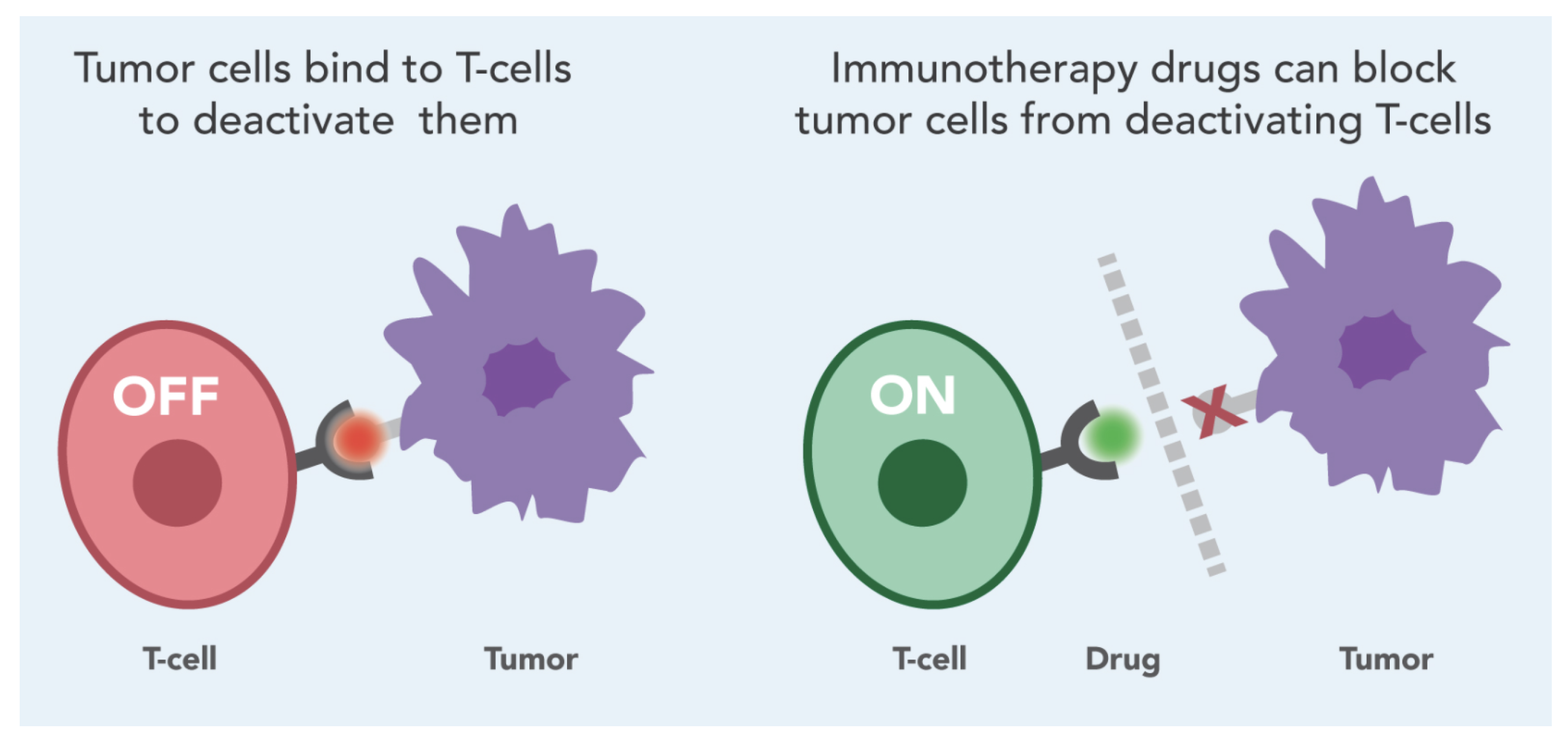
7.4. Immunotherapy

Immunotherapy is a type of cancer treatment that is intended to increase or improve the body’s natural immune responses. Unlike traditional medical help, it does not target the tumor but rather the host’s tumor-responding immune cells. The system (the human body’s anti-infection mechanisms) is made up of a network of cells, tissues, and organs that recognize and eliminate foreign invaders such as bacteria and viruses, as well as aberrant cells within the body. This strategy is mediated by the system’s ability to recognize the distinction between the “self” and “non-self.” The self denotes your own bodily tissues. The non-self refers to any aberrant cell or foreign invader, such as a bacteria or virus.

T cells defend us against infection. We are continually exposed to pathogens such as bacteria, viruses, and fungi throughout our daily lives. Every exposure might be fatal without T lymphocytes, commonly known as T cells. T cells have the ability to eliminate contaminated or malignant cells. The process of immune therapy is concisely represented in Figure 5.

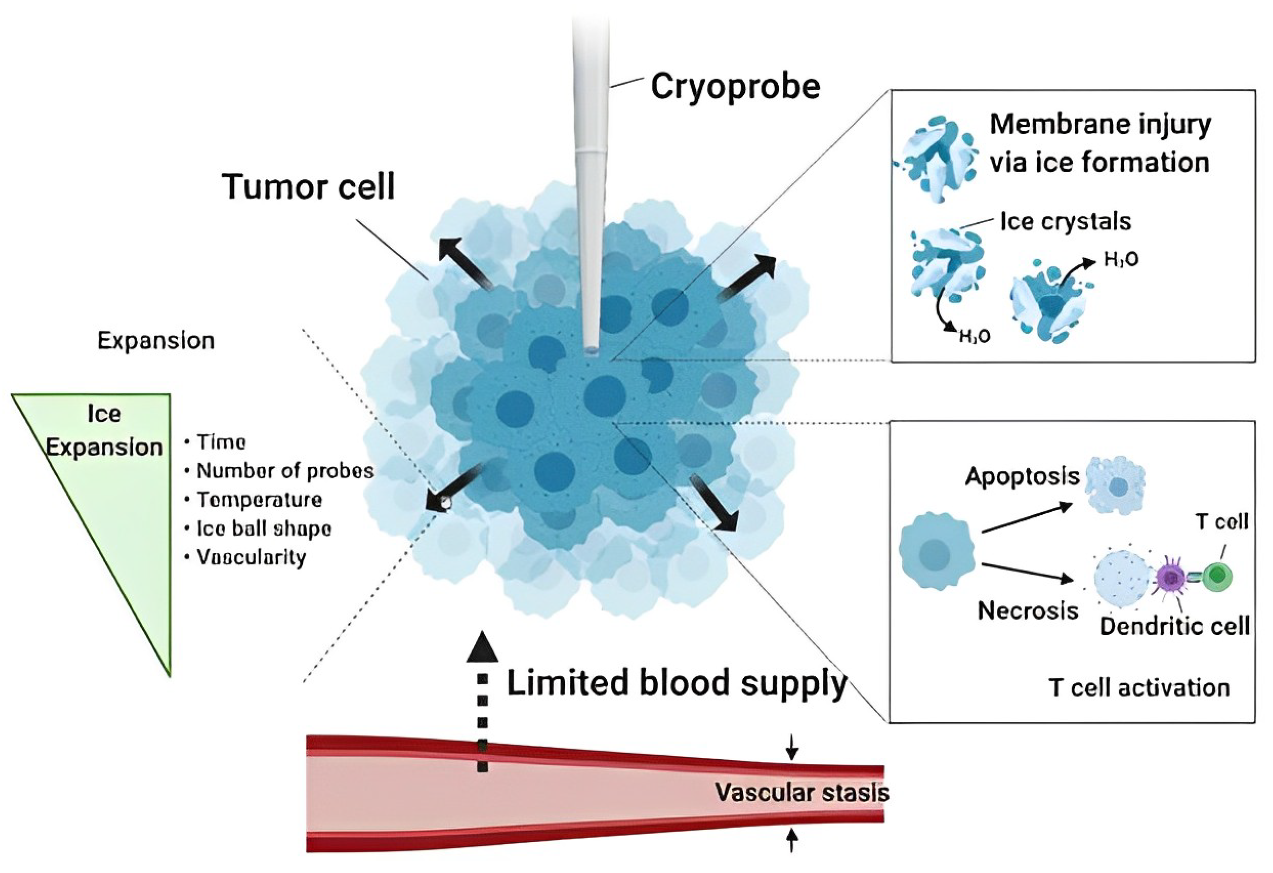
7.5. Cryoablation

In this therapy, the cold destroys the cancer cells. A slender, wand-like needle (cryoprobe) is introduced through the skin and straight into the malignant tumor during cryoablation. To freeze the tissue, a gas is fed into the cryoprobe. The tissue is then allowed to defrost. To the destroy cancer cells, the freezing and thawing process is performed numerous times during the same therapy session. Mechanisms of cryoablation are shown in Figure 6 at temperatures below $-20$ °C, intracellular ice develops, and cell death takes one of two forms: necrosis or apoptosis. Necrosis occurs when cellular membranes are disrupted, allowing tumor antigens to be phagocytozed by dendritic cells. The disruption of mitochondrial activity leads to the onset of Bax proteins, which drives downstream apoptotic pathways in apoptosis. Aside from the two primary processes of cell death, the development of an ice ball is affected by a variety of parameters, including the duration of the freeze–thaw cycle, the number of cryoprobes, the temperature, the shape of the ice ball, and the vascularity of the target ablation zone.

7.6. Proposed Strategy

In this section, a previously suggested treatment strategy is discussed.

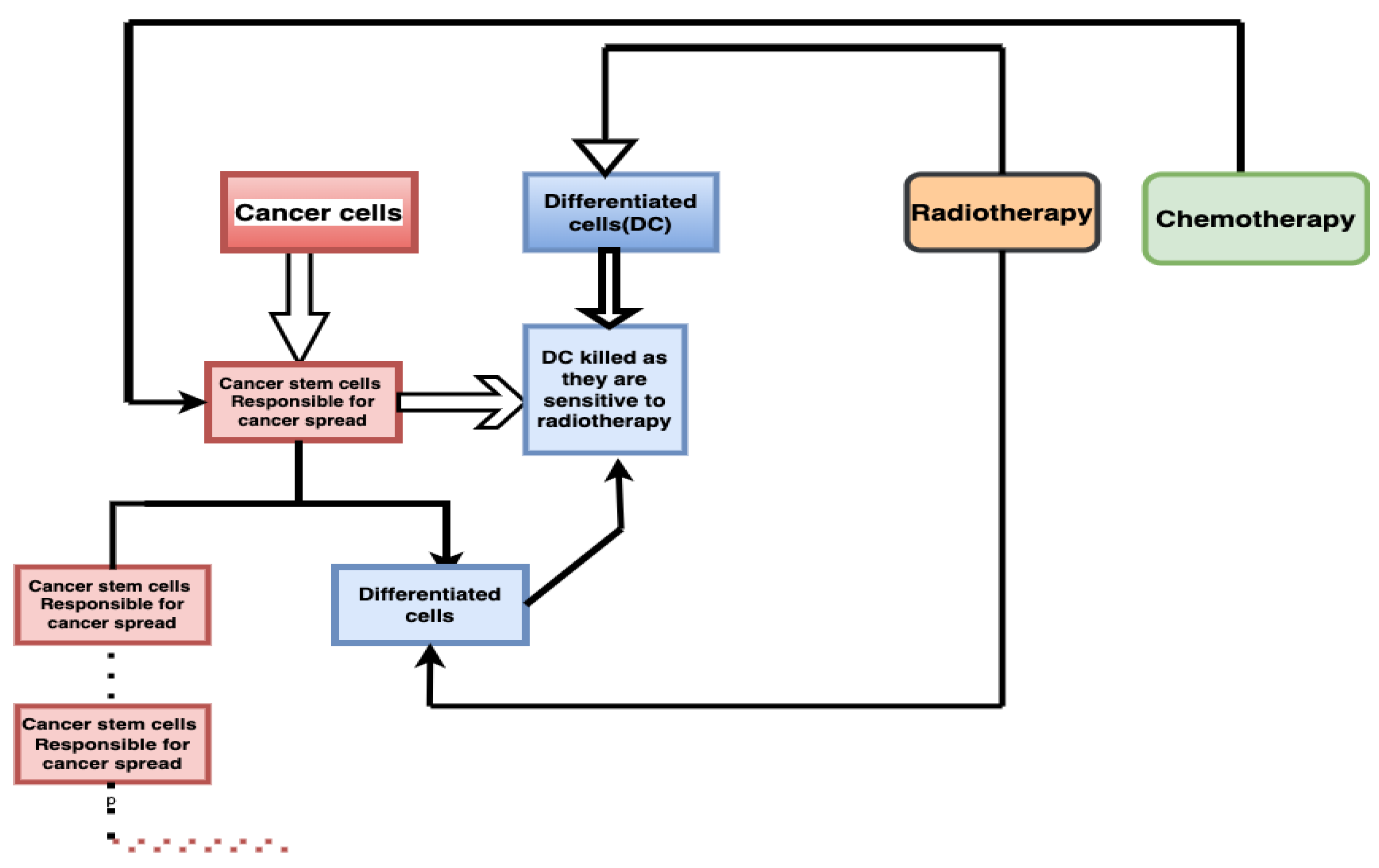
7.6.1. Treatment without Considering Heterogeneity of Cancer Cells

First, the previous treatments are discussed in the form of an algorithm to show that the previous strategies do not take into account that cancer cells are heterogeneous and must be treated according to cell biology. This has not been accounted for in previously employed treatment strategies. This kind of treatment is illustrated as under in Algorithm 2.

Algorithm 2 (Treatment without considering Heterogeneity of Cancer Cells)

Step 1: First, the total cancer cells are considered.          They are of two types: cancer stem cells (CSCs) and differentiated cells (DCs).          Total cancer cells are: CSCs + DCs

Step 2: Apply treatment of radio therapy on both CSCs and DCs.          As DCs are sensitive to radiotherapy, they will be killed:          CSC are resistant to radiotherapy and responsible for cancer cells.

Step 3: CSCs will further continue to spread and divide into CSCs and DCs.          This spread will continue.

In the flow chart given in the Figure 7 elaborate the strategy to treat cancer without taking care of the heterogeneity among cancer cells.

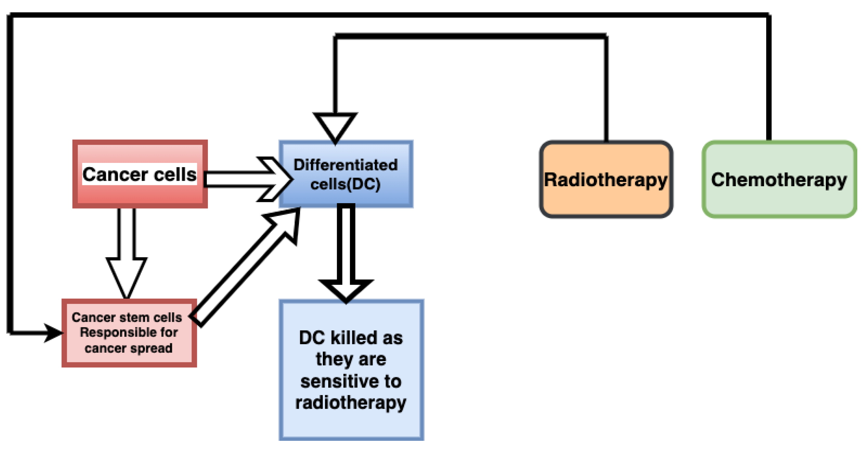
7.6.2. Suggested Treatment Strategy Accounting for Heterogeneity of Cells

The suggested treatment strategy accounting for heterogeneity of cancer cells is proposed is presented in the following Algorithm 3.

Algorithm 3 (Cancer treatment strategy accounting for Heterogeneity)

Step 1: First the total cancer cell are considered.          They are of two types: cancer stem cells (CSCs) and differentiated cells (DCs).          Total cancer cells are: CSCs + DCs

Step 2:          First apply chemotherapy; this will convert CSCs into DCs.          Meaning that it will convert radiotherapy-resistant cells (CSCs) into radiotherapy-sensitive cells (DCs).

Step 3:          Now apply radiotherapy and maximum cells will be killed as chemotherapy application makes the process of conversion of CSC into DC fast enough.

The flow chart shown in the Figure 8 explains our proposed strategy to cure cancer accounting for heterogeneity.

The Figure 9 is the simulation of the proposed stochastic model for cancer treatment, which has complete agreement with the Algorithm 3 that is, first it illustrates how cancer grows when no treatment is administered—it is shown that the cancer cells keep on increasing. As a result of chemotherapy, differentiated cells which are sensitive to radiotherapy are increased. Furthermore, one can finally easy observe how all types of cancer cells decreased as a result of radiotherapy. The Matlab code used to generate the simulation in the Figure 9 is given in the Appendix A.

Simulation of suggested model (1)

Figure 9. (A) Plot shows first that both stem (SCs) and differentiated cells (DCs) are increasing; (B) upon undertaking chemotherapy, the SCs decrease and the DCs increase; (C) upon undertaking radiotherapy, the total cancer decreases as DCs decrease due to radiotherapy. The interaction between C and D cells under radiotherapy is as follows: $C_0=\frac{2}{100}{10}^3$ cells, $D_0=\frac{1}{100}{10}^3$ cells, $\delta =0.4$ day ${}^{-1}$, $f=0.4$, $\mu =0.3$ day ${}^{-1}$, ${\alpha }_1=0.35$${Gy}^{-1}$, ${\alpha }_2=1.5$${Gy}^{-1}$, $\frac{{\alpha }_1}{{\beta }_1}=3$${Gy}^{-1}$, $\frac{{\alpha }_2}{{\beta }_2}=7$${Gy}^{-1}$, fractionated dose $=2$${Gy}^{-1}$ on week days.

Figure 9. (A) Plot shows first that both stem (SCs) and differentiated cells (DCs) are increasing; (B) upon undertaking chemotherapy, the SCs decrease and the DCs increase; (C) upon undertaking radiotherapy, the total cancer decreases as DCs decrease due to radiotherapy. The interaction between C and D cells under radiotherapy is as follows: $C_0=\frac{2}{100}{10}^3$ cells, $D_0=\frac{1}{100}{10}^3$ cells, $\delta =0.4$ day ${}^{-1}$, $f=0.4$, $\mu =0.3$ day ${}^{-1}$, ${\alpha }_1=0.35$${Gy}^{-1}$, ${\alpha }_2=1.5$${Gy}^{-1}$, $\frac{{\alpha }_1}{{\beta }_1}=3$${Gy}^{-1}$, $\frac{{\alpha }_2}{{\beta }_2}=7$${Gy}^{-1}$, fractionated dose $=2$${Gy}^{-1}$ on week days.

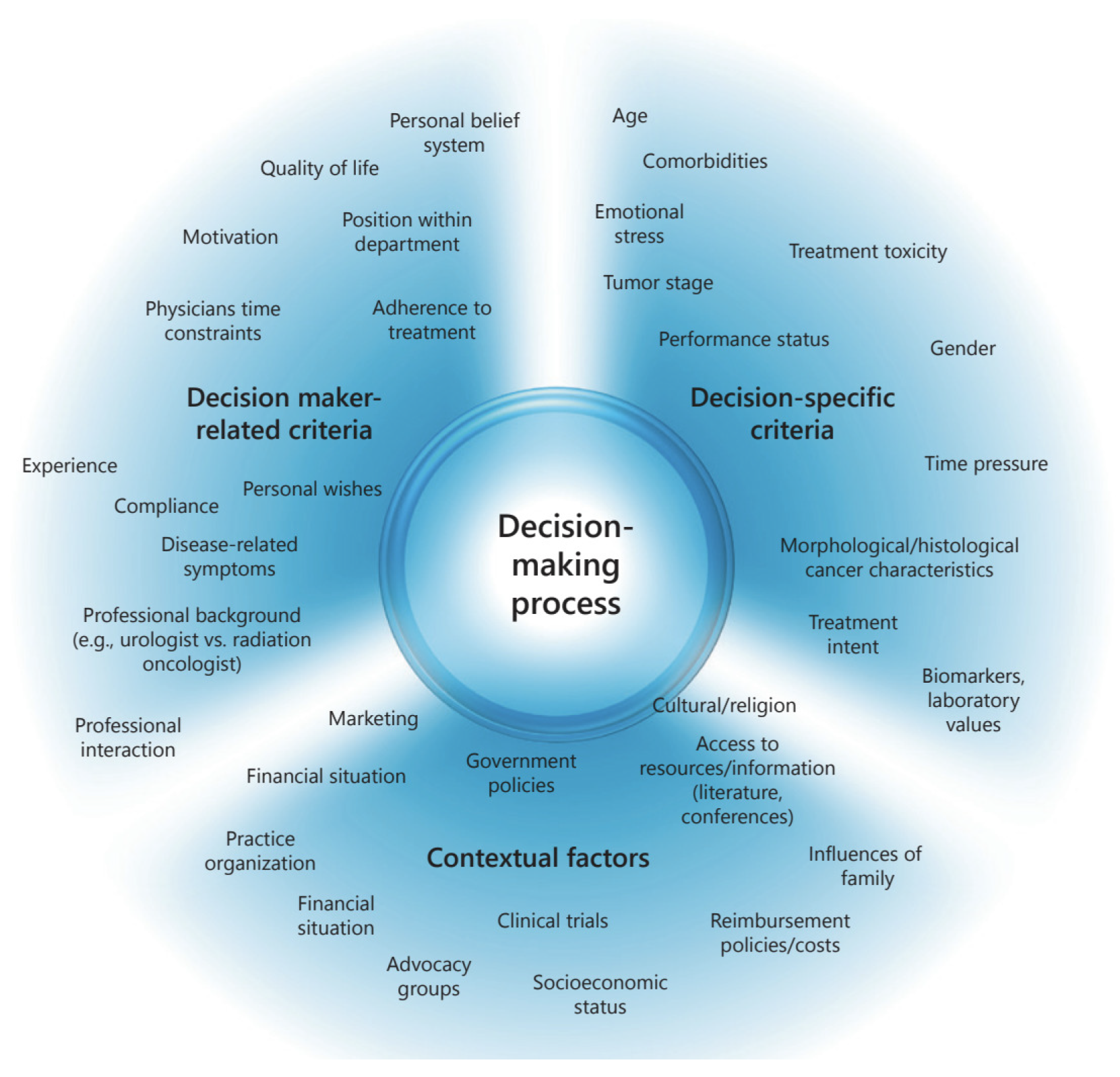
7.7. Decision-Making Criteria in Oncology

Clinical decision making is at the heart of regular clinical practice. Our opinions and conclusions are influenced by a variety of circumstances. Multiple alternatives for oncological problems are frequently available for a number of reasons [68]. Figure 10 shows the different factors involved in the decision-making process underlying the choice of cancer treatment.

(1)

In oncology, age is a main criteria in choosing the treatment for cancer. The treatment choice changes with the age of the patient. For example, radiation therapy is highly related to age [69]. Patients over 65 years of age may not tolerate all treatments as well as their younger counterparts.

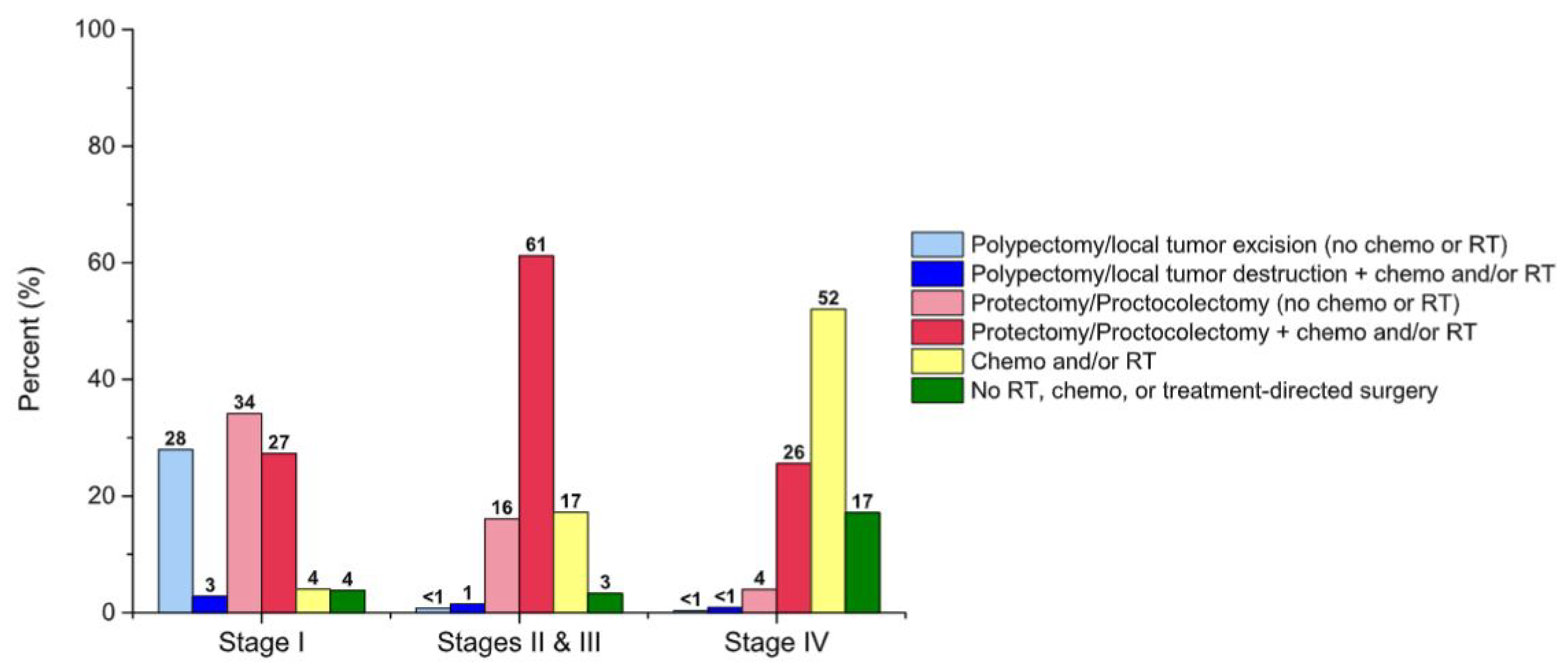
(2)

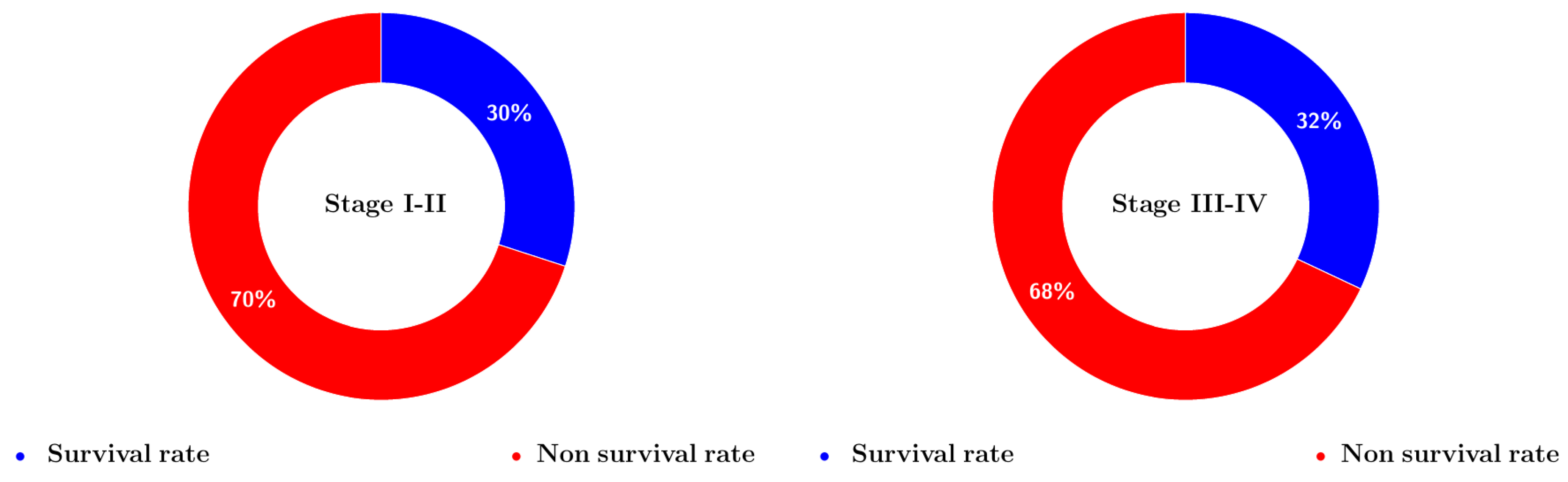
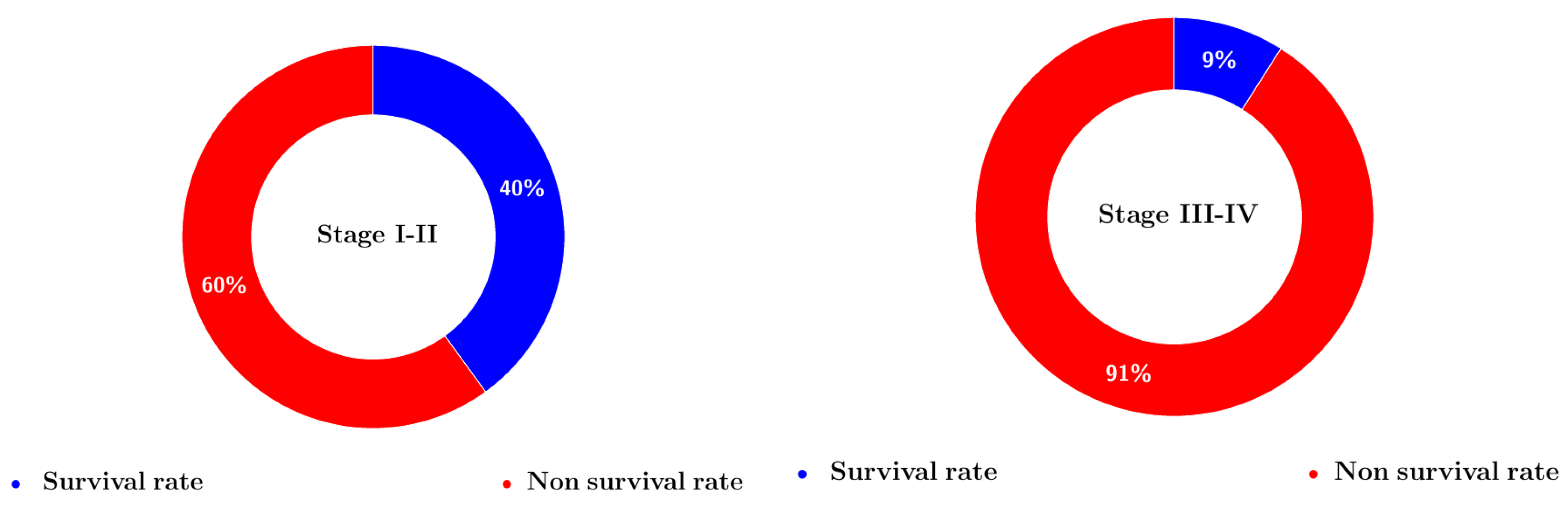
The cancer entity and stage are key factors to consider throughout the decision-making process. Treatment is mostly determined by the stage and extent of the cancer. The treatment guidelines for regionally based tumors differ from those for advanced sickness or metastasized tumors. The Figure 11 shows the relationship between stage of cancer and survival with respect to the choice of treatment [70].

(3)

The choice between prioritizing the quantity or quality of life will influence the decision of whether or not to treat, the degree of data available to support the option, and perhaps the level of adverse effects the patient is prepared to risk. The purpose of a technique determines the selection of decision criteria [71,72].

(4)

Cost is also an important factor when choosing cancer treatments. The resources of every individual are limited, and since saving a life is someone’s top priority, it is important to choose a life-saving treatment strategy considering the limited resources.

(5)

Long-term side effects are also an important factor to consider when choosing cancer treatment strategy.

Assume that a high-level group has been formed to decide how to improve cancer therapy in a state’s major cities. Five cancer therapy options are available, namely ${{\delta }^{\gimel }}_1$= chemotherapy, ${{\delta }^{\gimel }}_2=$ radiotherapy, ${{\delta }^{\gimel }}_3=$ immunotherapy, ${{\delta }^{\gimel }}_4$= cryoablation, and ${{\delta }^{\gimel }}_5=$ proposed strategy. This assessment group is composed of representatives from the ministries of healthcare, industry, and the environment. The panel is entrusted with evaluating cities based on five key criteria given in

Table 2. Criterion for the assessment.

	Criteria
${{\aleph }^{\delta }}_1$	Age
${{\aleph }^{\delta }}_2$	Type of cancer
${{\aleph }^{\delta }}_3$	Stage of the cancer
${{\aleph }^{\delta }}_4$	Cost of treatment
${{\aleph }^{\delta }}_5$	Chance of a cure

, throughout the three significant periods $d_1$, $d_2$, and $d_3$. Assume that $W=(0.15,0.10,0.25,0.20,0.30)$ represents the weighting of the criterion ${{\aleph }^{\delta }}_1$, ${{\aleph }^{\delta }}_2$, ${{\aleph }^{\delta }}_3$, ${{\aleph }^{\delta }}_4$, and ${{\aleph }^{\delta }}_5$, and that $\zeta \left(m_k\right)=(0.35,0.40,0.25)$ represents the weighting of the time periods $d_1$, $d_2$, and $d_3$. Assume that the experts construct a decision matrix table with dynamic q-RPFNs. This is carried out in the following order: Step 1 through Step 7 of the Algorithm.

7.8. Decision-Making Process

Step 1:

Acquire a decision or assessment matrix $R\left(m_k\right)={\left(r_{ij}^k\right)}_{m\times n}={\left({\delta }_{ij}^{\prime }\left(m_k\right),{\nu }_{ij}^{\prime }\left(m_k\right),{\lambda }_{ij}^{\prime }\left(m_k\right)\right)}_{m\times n}$ for the d different periods. The assessment matrix acquired from $d_1$ is given in

Table 3. Assessment matrix acquired from $d_1$.

	${{\mathit{\aleph }}^{\mathit{\delta }}}_1$	${{\mathit{\aleph }}^{\mathit{\delta }}}_2$	${{\mathit{\aleph }}^{\mathit{\delta }}}_3$	${{\mathit{\aleph }}^{\mathit{\delta }}}_4$	${{\mathit{\aleph }}^{\mathit{\delta }}}_5$
${{\delta }^{\gimel }}_1$	(0.367,0.142,0.372)	(0.364,0.155,0.283)	(0.285,0.165,0.152)	(0.145,0.154,0.253)	(0.385,0.132,0.473)
${{\delta }^{\gimel }}_2$	(0.167,0.384,0.236)	(0.140,0.150,0.168)	(0.165,0.135,0.374)	(0.144,0.363,0.396)	(0.145,0.475,0.337)
${{\delta }^{\gimel }}_3$	(0.142,0.131,0.136)	(0.144,0.265,0.572)	(0.475,0.165,0.249)	(0.473,0.166,0.138)	(0.375,0.142,0.399)
${{\delta }^{\gimel }}_4$	(0.464,0.163,0.172)	(0.485,0.175,0.152)	(0.175,0.253,0.299)	(0.155,0.242,0.393)	(0.455,0.353,0.248)
${{\delta }^{\gimel }}_5$	(0.353,0.266,0.239)	(0.133,0.175,0.131)	(0.175,0.125,0.493)	(0.384,0.155,0.493)	(0.142,0.363,0.395)

.

The assessment matrix acquired from $d_2$ is given in

Table 4. Assessment matrix acquired from $d_2$.

	${{\mathit{\aleph }}^{\mathit{\delta }}}_1$	${{\mathit{\aleph }}^{\mathit{\delta }}}_2$	${{\mathit{\aleph }}^{\mathit{\delta }}}_3$	${{\mathit{\aleph }}^{\mathit{\delta }}}_4$	${{\mathit{\aleph }}^{\mathit{\delta }}}_5$
${{\delta }^{\gimel }}_1$	(0.384,0.155,0.142)	(0.245,0.133,0.231)	(0.465,0.155,0.375)	(0.167,0.165,0.172)	(0.235,0.155,0.188)
${{\delta }^{\gimel }}_2$	(0.165,0.125,0.285)	(0.350,0.245,0.147)	(0.155,0.280,0.134)	(0.455,0.345,0.124)	(0.152,0.140,0.182)
${{\delta }^{\gimel }}_3$	(0.353,0.170,0.395)	(0.175,0.145,0.153)	(0.145,0.255,0.166)	(0.163,0.282,0.171)	(0.442,0.135,0.227)
${{\delta }^{\gimel }}_4$	(0.277,0.464,0.173)	(0.165,0.166,0.132)	(0.125,0.140,0.157)	(0.280,0.272,0.237)	(0.489,0.135,0.382)
${{\delta }^{\gimel }}_5$	(0.151,0.136,0.182)	(0.280,0.494,0.131)	(0.175,0.242,0.182)	(0.384,0.182,0.182)	(0.153,0.246,0.151)

.

The assessment matrix acquired from $d_3$ is given in

Table 5. Assessment matrix acquired from $d_3$.

	${{\mathit{\aleph }}^{\mathit{\delta }}}_1$	${{\mathit{\aleph }}^{\mathit{\delta }}}_2$	${{\mathit{\aleph }}^{\mathit{\delta }}}_3$	${{\mathit{\aleph }}^{\mathit{\delta }}}_4$	${{\mathit{\aleph }}^{\mathit{\delta }}}_5$
${{\delta }^{\gimel }}_1$	(0.134,0.274,0.162)	(0.135,0.175,0.153)	(0.285,0.253,0.253)	(0.253,0.145,0.153)	(0.162,0.253,0.156)
${{\delta }^{\gimel }}_2$	(0.242,0.166,0.374)	(0.155,0.145,0.192)	(0.144,0.165,0.137)	(0.463,0.130,0.148)	(0.134,0.134,0.145)
${{\delta }^{\gimel }}_3$	(0.134,0.155,0.142)	(0.131,0.165,0.153)	(0.135,0.490,0.264)	(0.263,0.145,0.489)	(0.242,0.253,0.375)
${{\delta }^{\gimel }}_4$	(0.166,0.384,0.373)	(0.353,0.275,0.153)	(0.165,0.155,0.197)	(0.255,0.155,0.264)	(0.135,0.164,0.153)
${{\delta }^{\gimel }}_5$	(0.145,0.266,0.133)	(0.285,0.195,0.486)	(0.310,0.155,0.174)	(0.145,0.155,0.247)	(0.283,0.245,0.486)

.

Step 2:

Normalize the decision matrices acquired by DMs using Equation (13). Here, we have two types of criteria. ${{\aleph }^{\delta }}_4$ is the cost-type criteria and others are benefit-type criteria.

The normalized matrix acquired from $d_1$ is given in

Table 6. Normalized matrix acquired from $d_1$.

	${{\mathit{\aleph }}^{\mathit{\delta }}}_1$	${{\mathit{\aleph }}^{\mathit{\delta }}}_2$	${{\mathit{\aleph }}^{\mathit{\delta }}}_3$	${{\mathit{\aleph }}^{\mathit{\delta }}}_4$	${{\mathit{\aleph }}^{\mathit{\delta }}}_5$
${{\delta }^{\gimel }}_1$	(0.467,0.242,0.472)	(0.464,0.255,0.383)	(0.385,0.265,0.252)	(0.254,0.353,0.245)	(0.485,0.232,0.573)
${{\delta }^{\gimel }}_2$	(0.267,0.484,0.336)	(0.240,0.250,0.268)	(0.265,0.235,0.474)	(0.463,0.496,0.244)	(0.245,0.575,0.437)
${{\delta }^{\gimel }}_3$	(0.242,0.231,0.236)	(0.244,0.365,0.672)	(0.575,0.265,0.349)	(0.266,0.238,0.573)	(0.475,0.242,0.499)
${{\delta }^{\gimel }}_4$	(0.564,0.263,0.272)	(0.585,0.275,0.252)	(0.275,0.353,0.399)	(0.342,0.493,0.255)	(0.555,0.453,0.348)
${{\delta }^{\gimel }}_5$	(0.453,0.366,0.339)	(0.233,0.275,0.231)	(0.275,0.225,0.593)	(0.255,0.593,0.484)	(0.242,0.463,0.495)

.

The normalized matrix acquired from $d_2$ is given in

Table 7. Normalized matrix acquired from $d_2$.

	${{\mathit{\aleph }}^{\mathit{\delta }}}_1$	${{\mathit{\aleph }}^{\mathit{\delta }}}_2$	${{\mathit{\aleph }}^{\mathit{\delta }}}_3$	${{\mathit{\aleph }}^{\mathit{\delta }}}_4$	${{\mathit{\aleph }}^{\mathit{\delta }}}_5$
${{\delta }^{\gimel }}_1$	(0.484,0.255,0.242)	(0.345,0.233,0.331)	(0.565,0.255,0.475)	(0.265,0.272,0.267)	(0.335,0.255,0.288)
${{\delta }^{\gimel }}_2$	(0.265,0.225,0.385)	(0.450,0.345,0.247)	(0.255,0.380,0.234)	(0.445,0.224,0.555)	(0.252,0.240,0.282)
${{\delta }^{\gimel }}_3$	(0.453,0.270,0.495)	(0.275,0.245,0.253)	(0.245,0.355,0.266)	(0.382,0.271,0.263)	(0.542,0.235,0.327)
${{\delta }^{\gimel }}_4$	(0.377,0.564,0.273)	(0.265,0.266,0.232)	(0.225,0.240,0.257)	(0.372,0.337,0.380)	(0.589,0.235,0.482)
${{\delta }^{\gimel }}_5$	(0.251,0.236,0.282)	(0.380,0.594,0.231)	(0.275,0.342,0.282)	(0.282,0.282,0.484)	(0.253,0.346,0.251)

.

The normalized matrix acquired from $d_1$ is given in

Table 8. Normalized matrix acquired from $d_3$.

	${{\mathit{\aleph }}^{\mathit{\delta }}}_1$	${{\mathit{\aleph }}^{\mathit{\delta }}}_2$	${{\mathit{\aleph }}^{\mathit{\delta }}}_3$	${{\mathit{\aleph }}^{\mathit{\delta }}}_4$	${{\mathit{\aleph }}^{\mathit{\delta }}}_5$
${{\delta }^{\gimel }}_1$	(0.234,0.374,0.262)	(0.235,0.275,0.253)	(0.385,0.353,0.353)	(0.245,0.253,0.353)	(0.262,0.353,0.256)
${{\delta }^{\gimel }}_2$	(0.342,0.266,0.474)	(0.255,0.245,0.292)	(0.244,0.265,0.237)	(0.230,0.248,0.563)	(0.234,0.234,0.245)
${{\delta }^{\gimel }}_3$	(0.234,0.255,0.242)	(0.231,0.265,0.253)	(0.235,0.590,0.364)	(0.245,0.589,0.363)	(0.342,0.353,0.475)
${{\delta }^{\gimel }}_4$	(0.266,0.484,0.473)	(0.453,0.375,0.253)	(0.265,0.255,0.297)	(0.255,0.364,0.355)	(0.235,0.264,0.253)
${{\delta }^{\gimel }}_5$	(0.245,0.366,0.233)	(0.385,0.295,0.586)	(0.410,0.255,0.274)	(0.255,0.347,0.245)	(0.383,0.345,0.586)

.

Step 3:

In this step, we utilized the proposed q-RPFDEWA operator to aggregate all the normalized decision matrices $N\left(m_k\right)={\left(n_{ij}^k\right)}_{m\times n}={\left({\delta }_{ij}\left(m_k\right),{\nu }_{ij}\left(m_k\right),{\lambda }_{ij}\left(m_k\right)\right)}_{m\times n}$ into one cumulative q-RPF matrix $Z={\left(z_{ij}\right)}_{m\times n}={\left({\delta }_{ij},{\nu }_{ij},{\lambda }_{ij}\right)}_{m\times n}$.

Step 4:

Define $A^{+}={({{\alpha }^{\hslash }}^{+1},{{\alpha }^{\hslash }}^{+2},\dots ,{{\alpha }^{\hslash }}^{+m})}^T$ and $A^{-}={({{\alpha }^{\hslash }}^{-1},{{\alpha }^{\hslash }}^{-2},\dots ,{{\alpha }^{\hslash }}^{-m})}^T$ as the q-RPF positive ideal solution (q-RPFPIS) and the q-RPF negative ideal solution (q-RPFNIS) as

$$\begin{array}{cc}& A^{+}=((1,0,0),(1,0,0),(1,0,0),(1,0,0),(1,0,0)),\hfill \\ & A^{-}=((0,0,1),(0,0,1),(0,0,1),(0,0,1),(0,0,1)).\hfill \end{array}$$

and

${{\delta }^{\gimel }}_1=((0.445253,0.281624,0.301029),(0.386485,0.251598,0.319061),(0.48957,0.284412,0.359481),(0.256243,0.287820,0.282953),(0.398981,0.273292,0.339379))$

${{\delta }^{\gimel }}_2=((0.297577,0.297896,0.393483),(0.380198,0.282677,0.266157),(0.255217,0.295307,0.290462),$$(0.423090,0.293360,0.436597),(0.244948,0.310085,0.308407))$

${{\delta }^{\gimel }}_3=((0.381590,0.253276,0.316056),(0.255363,0.282726,0.288560),(0.454748,0.379352,0.317078),$$(0.330077,0.329611,0.366467),(0.486936,0.267879,0.415438))$

${{\delta }^{\gimel }}_4=((0.459936,0.429227,0.321736),(0.484967,0.271364,0.244091),(0.255768,0.274417,0.306307),$$(0.340494,0.386724,0.330368),(0.536387,0.296427,0.360495))$

${{\delta }^{\gimel }}_5=((0.363962,0.279072,0.281441),(0.358396,0.383055,0.305997),(0.340495,0.276223,0.350056),$$(0.267132,0.375715,0.394955),(0.315702,0.377352,0.397659))$

Step 5 and Step 6:

Calculate the distance between the alternative ${{\delta }^{\gimel }}_i$ and the q-RPFPIS $A^{+}$ and the distance between the alternative ${{\delta }^{\gimel }}_i$ and the q-RPFNIS $A^{-}$, respectively. Then, we calculate the closeness coefficient of each alternative:

$$c\left({{\delta }^{\gimel }}_1\right)=0.246842$$

$$c\left({{\delta }^{\gimel }}_2\right)=0.444742$$

$$c\left({{\delta }^{\gimel }}_3\right)=0.353512$$

$$c\left({{\delta }^{\gimel }}_4\right)=0.424229$$

$$c\left({{\delta }^{\gimel }}_5\right)=0.533421$$

Step 7:

Rank all the alternatives ${{\delta }^{\gimel }}_i(i=1,2,\cdots ,n)$ according to the closeness coefficients $c\left({{\delta }^{\gimel }}_i\right)(i=1,2,\cdots ,n)$

$${{\delta }^{\gimel }}_5>{{\delta }^{\gimel }}_2>{{\delta }^{\gimel }}_4>{{\delta }^{\gimel }}_3>{{\delta }^{\gimel }}_1.$$

7.9. Limitations of the Proposed Method

To demonstrate the inadequacies of the given techniques, we conducted a critical analysis of the algorithm and listed its disadvantages:

• Logical dependencies amongst the parameters were ignored in the preceding instances.
• In practice, it is not generally fair to suggest that each parameter in the MPDM is independent of the others. Any parameter in the MPDM may be reliant on or connected to other parameters.
• Evaluation of parameter dependencies should add to the objectivity of judgments in the suggested MPDM techniques. The consideration of dependence in the q-RPF MPDM may increase the decision-making framework’s quality.

7.10. Authenticity Analysis

Wang and Triantaphyllou [73] evaluated the preceding test criteria to demonstrate the effectiveness of the suggested technique:

• Test 1: If we replace the non-optimal alternate’s grade values with those of the worst choice, the ideal option should not change as long as the respective priority relationship remains unchanged.
• Test 2: The approach’s framework should be transitive.
• Test 3: Whenever a continuous dilemma is partitioned and the same MCDM algorithm is used, the accumulated rating of the alternatives must be comparable to the initial problem’s evaluation.

We checked the constraints on our proposed MCDM technique in the subsection below.

7.10.1. Authenticity Test 1

Here, we used the q-RPFDEWA operator in this test if we exchange the PMSGs and N ${}_g$ MSGs of alternatives ${{\delta }^{\gimel }}_4$ and ${{\delta }^{\gimel }}_1$ in

Table 9. Aggregated values.

	${{\mathit{\aleph }}^{\mathit{\delta }}}_1$	${{\mathit{\aleph }}^{\mathit{\delta }}}_2$	${{\mathit{\aleph }}^{\mathit{\delta }}}_3$
${{\delta }^{\gimel }}_1$	(0.445253, 0.281624, 0.301029)	(0.386485, 0.251598, 0.319061)	(0.48957, 0.284412, 0.359481)
${{\delta }^{\gimel }}_2$	(0.297577, 0.297896, 0.393483)	(0.380198, 0.282677, 0.266157)	(0.255217, 0.295307, 0.290462)
${{\delta }^{\gimel }}_3$	(0.381590, 0.253276, 0.316056)	(0.255363, 0.282726, 0.288560)	(0.454748, 0.379352, 0.317078)
${{\delta }^{\gimel }}_4$	(0.459936, 0.429227, 0.321736)	(0.484967, 0.271364, 0.244091)	(0.255768, 0.274417, 0.306307)
${{\delta }^{\gimel }}_5$	(0.363962, 0.279072, 0.281441)	(0.358396, 0.383055, 0.305997)	(0.340495, 0.276223, 0.350056)
	${{\aleph }^{\delta }}_4$	${{\aleph }^{\delta }}_5$
${{\delta }^{\gimel }}_1$	$(0.256243,0.287820,0.282953)$	$(0.398981,0.273292,0.339379)$
${{\delta }^{\gimel }}_2$	$(0.423090,0.293360,0.436597)$	$(0.244948,0.310085,0.308407)$
${{\delta }^{\gimel }}_3$	$(0.330077,0.329611,0.366467)$	$(0.486936,0.267879,0.415438)$
${{\delta }^{\gimel }}_4$	$(0.340494,0.386724,0.330368)$	$(0.536387,0.296427,0.360495)$
${{\delta }^{\gimel }}_5$	$(0.267132,0.375715,0.394955)$	$(0.315702,0.377352,0.397659)$

.

The suggested q-RPFDEWA operator has been implemented based on this information. Thus, the ranking arrangement of the alternatives dependent on the score values is ${{\delta }^{\gimel }}_5>{{\delta }^{\gimel }}_2>{{\delta }^{\gimel }}_4>{{\delta }^{\gimel }}_3>{{\delta }^{\gimel }}_1$, which is the same as the initial decision-making ranking. As a result, the proposed methodology meets the first test condition. In the same way, we also check the q-RPFDEWG operator.

7.10.2. Authenticity Test 2 and Test 3

If we breakdown the provided problem into the sub-problems $\{{{\delta }^{\gimel }}_5,{{\delta }^{\gimel }}_2\}$, $\{{{\delta }^{\gimel }}_2,{{\delta }^{\gimel }}_4\}$, $\{{{\delta }^{\gimel }}_4,{{\delta }^{\gimel }}_3\}$, $\{{{\delta }^{\gimel }}_3,{{\delta }^{\gimel }}_1\}$, and $\{{{\delta }^{\gimel }}_1,{{\delta }^{\gimel }}_5\}$ then we apply the procedure steps of the proposed technique and we receive the ranking order of these smaller problems as ${{\delta }^{\gimel }}_5⪰{{\delta }^{\gimel }}_2$, ${{\delta }^{\gimel }}_2⪰{{\delta }^{\gimel }}_4$, ${{\delta }^{\gimel }}_4⪰{{\delta }^{\gimel }}_3$, ${{\delta }^{\gimel }}_3⪰{{\delta }^{\gimel }}_1$, and ${{\delta }^{\gimel }}_5⪰{{\delta }^{\gimel }}_1$. As a result of merging them, the total ranking order of the alternate is ${{\delta }^{\gimel }}_5>{{\delta }^{\gimel }}_2>{{\delta }^{\gimel }}_4>{{\delta }^{\gimel }}_3>{{\delta }^{\gimel }}_1$, which is the same as the original ranking order. As a result, the proposed methodology meets authenticity test requirements 2 and 3.

8. Conclusions and Discussion

Cancer is a complicated disease and it spreads through the cells in the body. There are various therapies available to kill cancer cells. These therapies did not take into consideration that cell division is often an asymmetric process that can be thought of as a series of symmetry-breaking events. In the proposed strategy, the heterogeneity in the cancer cells is presented. Furthermore, mathematical models using the stochastic differential equations and stochastic delay differential equations of cancer cells in a tumor bulk were constructed. Two types of cells have been considered, namely cancer stem cells (CSCs), which are less sensitive, and differentiated cancer cells (DCs), which are more sensitive with respect to radiotherapy. Consecutive chemotherapy and radiotherapy were applied, with the aim of first converting CSCs into DCs, thus, making them more radio-sensitive with respect to treatment, then cell killing with radiotherapy in order to control and kill the tumor cells. With the help of simulation, it was demonstrated that the proposed strategy is very effective in order to kill cancer in a speedy manner because time is an important factor in curing cancer. Although information aggregation is significant during the decision-making process, numerous dynamic q-rung picture fuzzy AOs are designed to aggregate the q-RPF information accumulated over time. These include the q-rung picture fuzzy dynamic Einstein-weighted averaging and q-rung picture fuzzy dynamic Einstein-weighted geometric operators. All of the operators include time in the aggregation process and are thus time-dependent, which addresses some of the limitations of traditional static q-RPF aggregation operators. The proposed operators have been proven to have a variety of desirable characteristics. Finally, an example is provided to exemplify the dynamic operators and developed approach. The proposed method can be used to develop future dynamic decision-making methods such as dynamic confidential short-listing, medical assessment for COVID-19 task allocation, a dynamic financing approach, online social media surveillance, and dynamic military management assessment, as well as complex fuzzy dynamic decision making.

References

- Fedorov, A.; Clunie, D.; Ulrich, E.; Bauer, C.; Wahle, A.; Brown, B.B. DICOM for quantitative imaging biomarker development: A standards based approach to sharing clinical data and structured PET/CT analysis results in head and neck cancer research. PeerJ 2016, 4, e2057. [Google Scholar] [CrossRef] [PubMed] [Green Version]
- Sheergojri, A.R.; Iqbal, P.; Agarwal, P.; Ozdemir, N. Uncertainty-based Gompertz growth model for tumor population and its numerical analysis. Int. J. Optim. Control Theor. Appl. IJOCTA 2022, 12, 137–150. [Google Scholar] [CrossRef]
- Nopour, R.; Shanbehzadeh, M.; Kazemi-Arpanahi, H. Developing a clinical decision support system based on the fuzzy logic and decision tree to predict colorectal cancer. Med. J. Islam. Repub. Iran 2021, 35, 44. [Google Scholar] [CrossRef] [PubMed]
- Balis, F.M. The goal of cancer treatment. Oncologist 1998, 3. [Google Scholar] [CrossRef] [Green Version]
- Zadeh, L.A. Fuzzy sets. Inf. Control 1965, 8, 338–353. [Google Scholar] [CrossRef] [Green Version]
- Atanassov, K.T. Intuitionistic fuzzy sets. Fuzzy Sets Syst. 1986, 20, 87–96. [Google Scholar] [CrossRef]
- Cuong, B.C.; Kreinovich, V. Picture fuzzy sets—A new concept for computational intelligence problems. In Proceedings of the 2013 Third World Congress on Information and Communication Technologies (WICT 2013), Hanoi, Vietnam, 15–18 December 2013; IEEE: Hanoi, Vietnam, 2013; pp. 1–6. [Google Scholar]
- Cuong, B.C. Picture fuzzy sets. J. Comput. Sci. Technol. 2014, 30, 409–420. [Google Scholar]
- Wei, G.; Alsaadi, F.E.; Hayat, T.; Alsaedi, A. Projection models for multiple attribute decision making with picture fuzzy information. Int. J. Mach. Learn. Cybern. 2018, 9, 713–719. [Google Scholar] [CrossRef]
- Wei, G.; Gao, H. The generalized Dice similarity measures for picture fuzzy sets and their applications. Informatica 2018, 29, 107–124. [Google Scholar] [CrossRef] [Green Version]
- Wei, G. Some similarity measures for picture fuzzy sets and their applications. Iran. J. Fuzzy Syst. 2018, 15, 77–89. [Google Scholar]
- Cuong, H.B.C.; Pham, V.H. Some fuzzy logic operators for picture fuzzy sets. In Proceedings of the Seventh International Conference on Knowledge and Systems Engineering, Yokohama, Japan, 10–12 June 2015; pp. 132–137. [Google Scholar]
- Phong, P.H.; Hieu, D.T.; Ngan, R.T.H.; Them, P.T. Some compositions of picture fuzzy relations. In Proceedings of the 7th National Conference on Fundamental and Applied Information Technology Research, FAIR’7, Thai Nguyen, Vietnam, 19–20 June 2014; pp. 19–20. [Google Scholar]
- Riaz, M.; Hashmi, M.R.; Pamucar, D.; Chu, Y.M. Spherical linear Diophantine fuzzy sets with modeling uncertainties in MCDM. Comput. Model. Eng. Sci. 2021, 126, 1125–1164. [Google Scholar] [CrossRef]
- Wang, R.; Wang, J.; Gao, H.; Wei, G. Methods for MADM with picture fuzzy muirhead mean operators and their application for evaluating the financial investment risk. Symmetry 2018, 11, 6. [Google Scholar] [CrossRef]
- Garg, H. Some picture fuzzy aggregation operators and their applications to multicriteria decision-making. Arab. J. Sci. Eng. 2017, 42, 5275–5290. [Google Scholar] [CrossRef]
- Tian, C.; Peng, J.J.; Zhang, S.; Zhang, W.Y.; Wang, J.Q. Weighted picture fuzzy aggregation operators and their applications to multi-criteria decision-making problems. Comput. Ind. Eng. 2019, 137, 106037. [Google Scholar] [CrossRef]
- Wei, G.W. Picture fuzzy hamacher aggregation operators and their application to multiple attribute decision making. Fundam. Informaticae 2018, 157, 271–320. [Google Scholar] [CrossRef]
- Jana, C.; Senapati, T.; Pal, M.; Yager, R.R. Picture fuzzy Dombi aggregation operators: Application to MADM process. Appl. Soft Comput. 2019, 74, 99–109. [Google Scholar] [CrossRef]
- Wang, L.; Zhang, H.Y.; Wang, J.Q.; Wu, G.F. Picture fuzzy multi-criteria group decision-making method to hotel building energy efficiency retrofit project selection. RAIRO-Oper. Res. 2020, 54, 211–229. [Google Scholar] [CrossRef] [Green Version]
- Riaz, M.; Farid, H.M.A. Hierarchical medical diagnosis approach for COVID-19 based on picture fuzzy fairly aggregation operators. Int. J. Biomath. 2022, 16, 2250075. [Google Scholar] [CrossRef]
- Naeem, M.; Khan, Y.; Ashraf, S.; Weera, W.; Batool, B. A novel picture fuzzy Aczel-Alsina geometric aggregation information: Application to determining the factors affecting mango crops. AIMS Math. 2022, 7, 12264–12288. [Google Scholar] [CrossRef]
- Farid, H.M.A.; Riaz, M. Some generalized q-rung orthopair fuzzy Einstein interactive geometric aggregation operators with improved operational laws. Int. J. Intell. Syst. 2021, 36, 7239–7273. [Google Scholar] [CrossRef]
- Saha, A.; Dutta, D.; Kar, S. Some new hybrid hesitant fuzzy weighted aggregation operators based on Archimedean and Dombi operations for multi-attribute decision making. Neural Comput. Appl. 2021, 33, 8753–8776. [Google Scholar] [CrossRef]
- Saha, A.; Majumder, P.; Dutta, D.; Debnath, B.K. Multi-attribute decision making using q-rung orthopair fuzzy weighted fairly aggregation operators. J. Ambient. Intell. Humaniz. Comput. 2011, 12, 8149–8171. [Google Scholar] [CrossRef]
- Akram, M.; Sattar, A.; Karaaslan, F.; Samanta, S. Extension of competition graphs under complex fuzzy environment. Complex Intell. Syst. 2021, 7, 539–558. [Google Scholar] [CrossRef]
- Karaaslan, F.; Ozlu, S. Correlation coefficients of dual type-2 hesitant fuzzy sets and their applications in clustering analysis. Int. J. Intell. Syst. 2020, 35, 1200–1229. [Google Scholar] [CrossRef]
- Alcantud, J.C.R. The relationship between fuzzy soft and soft topologies. J. Intell. Fuzzy Syst. 2022, 24, 1653–1668. [Google Scholar] [CrossRef]
- Kirişci, M.; Demir, I.; Şimşek, N. Fermatean fuzzy ELECTRE multi-criteria group decision-making and most suitable biomedical material selection. Artif. Intell. Med. 2022, 127, 102278. [Google Scholar] [CrossRef]
- Feng, F.; Fujita, H.; Ali, M.I.; Yager, R.R.; Liu, X. Another view on generalized intuitionistic fuzzy soft sets and related multiattribute decision making methods. IEEE Trans. Fuzzy Syst. 2018, 27, 474–488. [Google Scholar] [CrossRef]
- Mahmood, T.; Ullah, K.; Khan, Q.; Jan, N. An approach toward decision-making and medical diagnosis problems using the concept of spherical fuzzy sets. Neural Comput. Appl. 2019, 31, 7041–7053. [Google Scholar] [CrossRef]
- Ashraf, T.; Abdullah, S.T.; Mahmood, F.; Ghani, T.M. Spherical fuzzy sets and their applications in multi-attribute decision making problems. Int. J. Intell. Syst. 2019, 36, 2829–2844. [Google Scholar] [CrossRef]
- Gündoğdu, F.K.; Kahraman, C. A novel fuzzy TOPSIS method using emerging interval-valued spherical fuzzy sets. Eng. Appl. Artif. Intell. 2019, 85, 307–323. [Google Scholar] [CrossRef]
- Parimala, M.; Broumi, S.; Prakash, K.; Topal, S. Bellman–ford algorithm for solving shortest path problem of a network under picture fuzzy environment. Complex Intell. Syst. 2011, 7, 2373–2381. [Google Scholar] [CrossRef]
- Li, L.; Zhang, R.; Wang, J.; Shang, X.; Bai, K. A novel approach to multi-attribute group decision-making with q-rung picture linguistic information. Symmetry 2018, 10, 172. [Google Scholar] [CrossRef]
- Akram, M.; Shahzadi, G.; Alcantud, J.C.R. Multi-attribute decision-making with q-rung picture fuzzy information. Granul. Comput. 2022, 7, 197–215. [Google Scholar] [CrossRef]
- Pinar, A.; Boran, F.E. A novel distance measure on q-rung picture fuzzy sets and its application to decision making and classification problems. Artif. Intell. Rev. 2022, 55, 1317–1350. [Google Scholar] [CrossRef]
- He, J.; Wang, X.; Zhang, R.; Li, L. Some q-rung picture fuzzy Dombi Hamy Mean operators with their application to project assessment. Mathematics 2019, 7, 468. [Google Scholar] [CrossRef] [Green Version]
- Liu, P.; Shahzadi, G.; Akram, M. Specific types of q-rung picture fuzzy Yager aggregation operators for decision making. Int. J. Comput. Intell. Syst. 2020, 13, 1072–1091. [Google Scholar] [CrossRef]
- Kamacı, H.; Petchimuthu, S.; Akçetin, E. Dynamic aggregation operators and Einstein operations based on interval-valued picture hesitant fuzzy information and their applications in multi-period decision making. Comput. Appl. Math. 2021, 40, 1–52. [Google Scholar] [CrossRef]
- Yang, Z.; Li, J.; Huang, L.; Shi, Y. Developing dynamic intuitionistic normal fuzzy aggregation operators for multi-attribute decision-making with time sequence preference. Expert Syst. Appl. 2017, 82, 344–356. [Google Scholar] [CrossRef]
- Jana, C.; Pal, M.; Liu, P. Multiple attribute dynamic decision making method based on some complex aggregation functions in CQROF setting. Comput. Appl. Math. 2022, 41, 103. [Google Scholar] [CrossRef]
- Peng, D.H.; Wang, H. Dynamic hesitant fuzzy aggregation operators in multi-period decision making. Kybernetes 2014, 43, 715–736. [Google Scholar] [CrossRef]
- Gumus, S.; Bali, Q. Dynamic aggregation operators based on intuitionistic fuzzy tools and einstein operations. Fuzzy Inf. Eng. 2017, 9, 45–65. [Google Scholar] [CrossRef]
- Riaz, M.; Farid, H.M.A. Picture fuzzy aggregation approach with application to third-party logistic provider selection process. Rep. Mech. Eng. 2022, 3, 318–327. [Google Scholar] [CrossRef]
- Sahu, R.; Dash, S.R.; Das, S. Career selection of students using hybridized distance measure based on picture fuzzy set and rough set theory. Decis. Mak. Appl. Manag. Eng. 2021, 4, 104–126. [Google Scholar] [CrossRef]
- Vojinovic, N.; Stevic, Z.; Tanackov, I. A Novel IMF SWARA-FDWGA-PESTEL Analysis For Assessment Of Healthcare System. Oper. Res. Eng. Sci. Theory Appl. 2022, 5, 139–151. [Google Scholar] [CrossRef]
- Peng, X.D.; Yang, Y. Some results for Pythagorean fuzzy sets. Int. J. Intell. Syst. 2015, 30, 1133–1160. [Google Scholar] [CrossRef]
- Jana, C.; Pal, M.; Wang, J.Q. Bipolar fuzzy Dombi aggregation operators and its application in multiple-attribute decision-making process. J. Ambient. Intell. Humaniz. Comput. 2019, 10, 3533–3549. [Google Scholar] [CrossRef]
- Feng, F.; Zheng, Y.; Sun, B.; Akram, M. Novel score functions of generalized orthopair fuzzy membership grades with application to multiple attribute decision making. Granul. Comput. 2022, 7, 95–111. [Google Scholar] [CrossRef]
- Yager, R.R.; Abbasov, A.M. Pythagorean membership grades, complex numbers, and decision making. Int. J. Intell. Syst. 2013, 28, 436–452. [Google Scholar] [CrossRef]
- Yager, R.R. Generalized orthopair fuzzy sets. IEEE Trans. Fuzzy Syst. 2016, 25, 1222–1230. [Google Scholar] [CrossRef]
- Xu, Z.S. Intuitionistic fuzzy aggregation operators. IEEE Trans. Fuzzy Syst. 2007, 15, 1179–1187. [Google Scholar]
- Wei, G. Picture fuzzy aggregation operators and their application to multiple attribute decision making. J. Intell. Fuzzy Syst. 2017, 33, 713–724. [Google Scholar] [CrossRef]
- Liu, P.; Wang, P. Some q-rung orthopair fuzzy aggregation operators and their applications to multiple-attribute decision making. Int. J. Intell. Syst. 2018, 33, 259–280. [Google Scholar] [CrossRef]
- Magee, J.A.; Piskounova, E.; Morrison, S.J. Cancer stem cells: Impact, heterogeneity, and uncertainty. Cancer Cell 2012, 21, 283–296. [Google Scholar] [CrossRef] [PubMed]
- Lopez Alfonso, J.C.; Jagiella, N.; Nunez, L.; Herrero, M.A.; Drasdo, D. Estimating dose painting effects in radiotherapy: A mathematical model. PLoS ONE 2014, 9, e89380. [Google Scholar] [CrossRef]
- Jordan, C.T.; Guzman, M.L.; Noble, M. Cancer stem cells. N. Engl. J. Med. 2016, 355, 1253–1261. [Google Scholar] [CrossRef] [PubMed]
- Lobo, N.A.; Shimono, Y.; Qian, D.; Clarke, M.F. The biology of cancer stem cells. Annu. Rev. Cell Dev. Biol. 2007, 23, 675–699. [Google Scholar] [CrossRef] [Green Version]
- Blevins-Knabe, B. Early mathematical development: How the home environment matters. In Early Childhood Mathematics Skill Development in the Home Environment; Springer: Berlin/Heidelberg, Germany, 2016; pp. 7–28. [Google Scholar]
- Dawson, A.; Hillen, T. Derivation of the tumour control probability (TCP) from a cell cycle model. Comput. Math. Methods Med. 2006, 7, 121–141. [Google Scholar] [CrossRef] [Green Version]
- Gong, J. Tumor Control Probability Models. Ph.D. Thesis, University of Alberta, Edmonton, AB, USA, 2013. [Google Scholar]
- Ruddon, R.W. Cancer Biology; Oxford University Press: Oxford, UK, 2007. [Google Scholar]
- Rozek, L. S NPG services. Nat. Rev. Cancer 2005, 5, 588. [Google Scholar]
- Serkova, N.J.; Eckhardt, S.G. Metabolic imaging to assess treatment response to cytotoxic and cytostatic agents. Front. Oncol. 2016, 6, 152. [Google Scholar] [CrossRef] [PubMed] [Green Version]
- Gazda, M.J.; Coia, L.R. Principles of radiation therapy. In Cancer Management: A Multidisciplinary Approach; Oncology Group: Melville, NY, USA, 2001; Available online: http://thymic.org/uploads/reference_sub/02radtherapy.pdf (accessed on 15 June 2022).
- Nie, D. Cancer stem cell and niche. Front. Biosci. Sch. Ed. 2009, 2, 184–193. [Google Scholar] [CrossRef] [PubMed] [Green Version]
- Panje, C.M.; Glatzer, M.; Sirén, C.; Plasswilm, L. Putora PM: Treatment options in oncology. JCO Clin. Cancer Inform. 2018, 2, 1–10. [Google Scholar] [CrossRef]
- Martin, A.M.; Raabe, E.; Eberhart, C.; Cohen, K.J. Management of pediatric and adult patients with medulloblastoma. Curr. Treat. Options Oncol. 2014, 15, 581–594. [Google Scholar] [CrossRef]
- Miller, K.D.; Nogueira, L.; Mariotto, A.B.; Rowl, J.H.; Yabroff, K.R.; Alfano, C.M.; Siegel, R.L. Cancer treatment and survivorship statistics. CA Cancer J. Clin. 2019, 69, 363–385. [Google Scholar] [CrossRef] [PubMed] [Green Version]
- Decaestecker, K.; De Meerleer, G.; Ameye, F.; Fonteyne, V.; Lambert, B.; Joniau, S.; Ost, P. Surveillance or metastasis-directed Therapy for OligoMetastatic Prostate cancer recurrence (STOMP): Study protocol for a randomized phase II trial. BMC Cancer 2014, 14, 671. [Google Scholar] [CrossRef]
- Zappa, C.; Shaker, A.M. Non-small cell lung cancer: Current treatment and future advances. Transl. Lung Cancer Res. 2016, 5, 288. [Google Scholar] [CrossRef] [PubMed] [Green Version]
- Wang, X.; Triantaphyllou, E. Ranking irregularities when evaluating alternatives by using some ELECTRE methods. Omega 2008, 36, 45–63. [Google Scholar] [CrossRef]