

The Exact Solutions of Fractional Differential Systems with n Sinusoidal Terms under Physical Conditions

Abstract
:1. Introduction
2. Analysis
3. Solution of the Fractional Models:
4. Solution of the Classical/Ordinary Models:
4.1. Class (1)
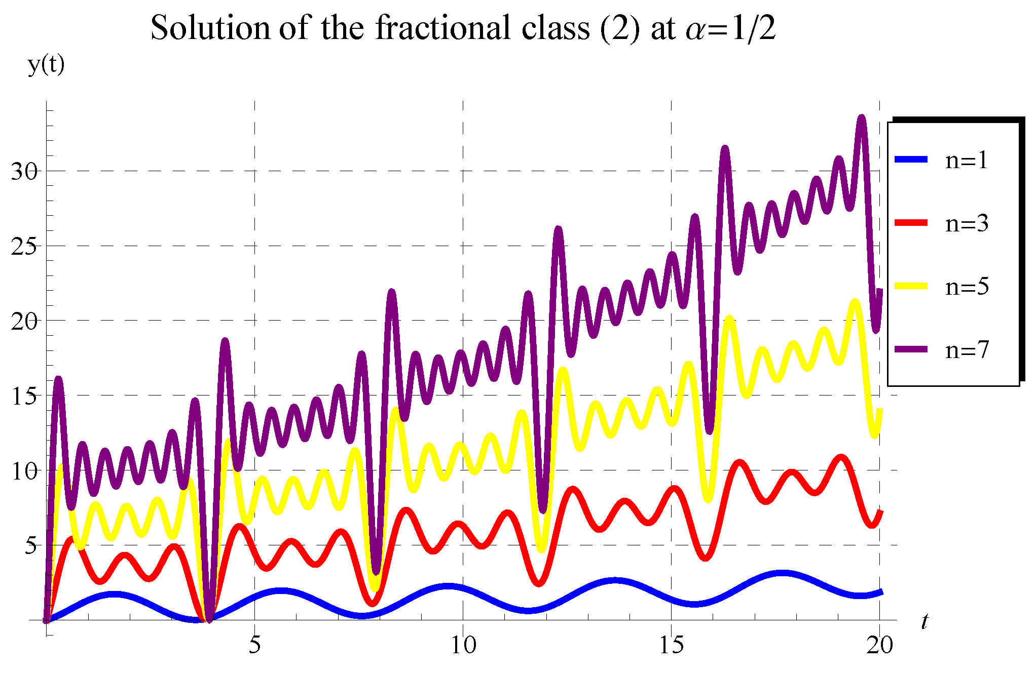
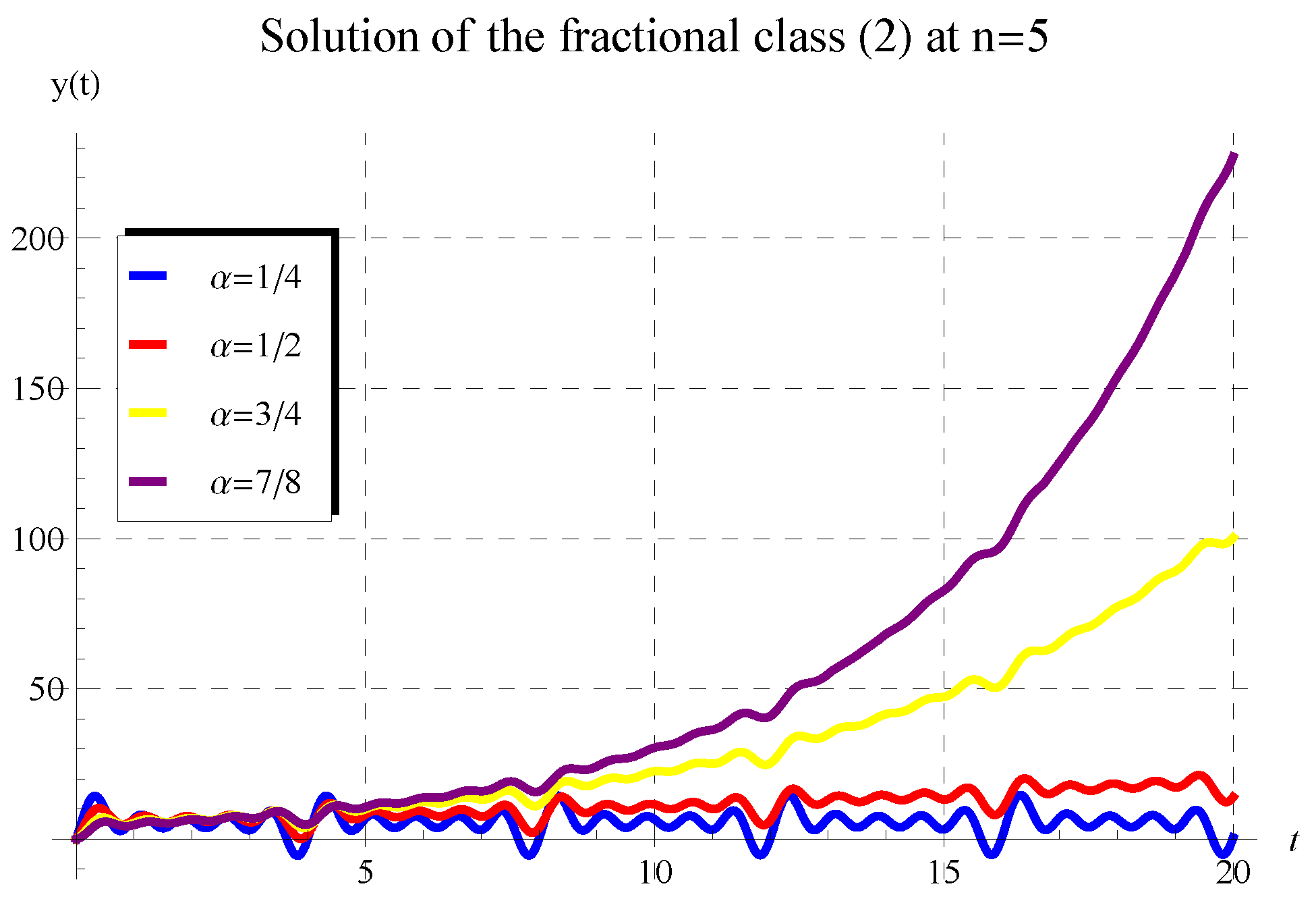
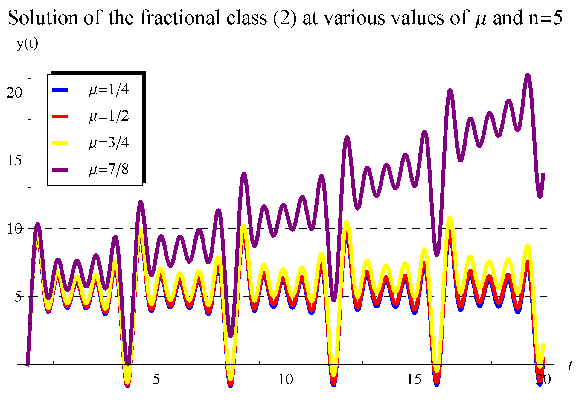
4.2. Class (2)
4.3. Class (3)
4.4. Class (4)
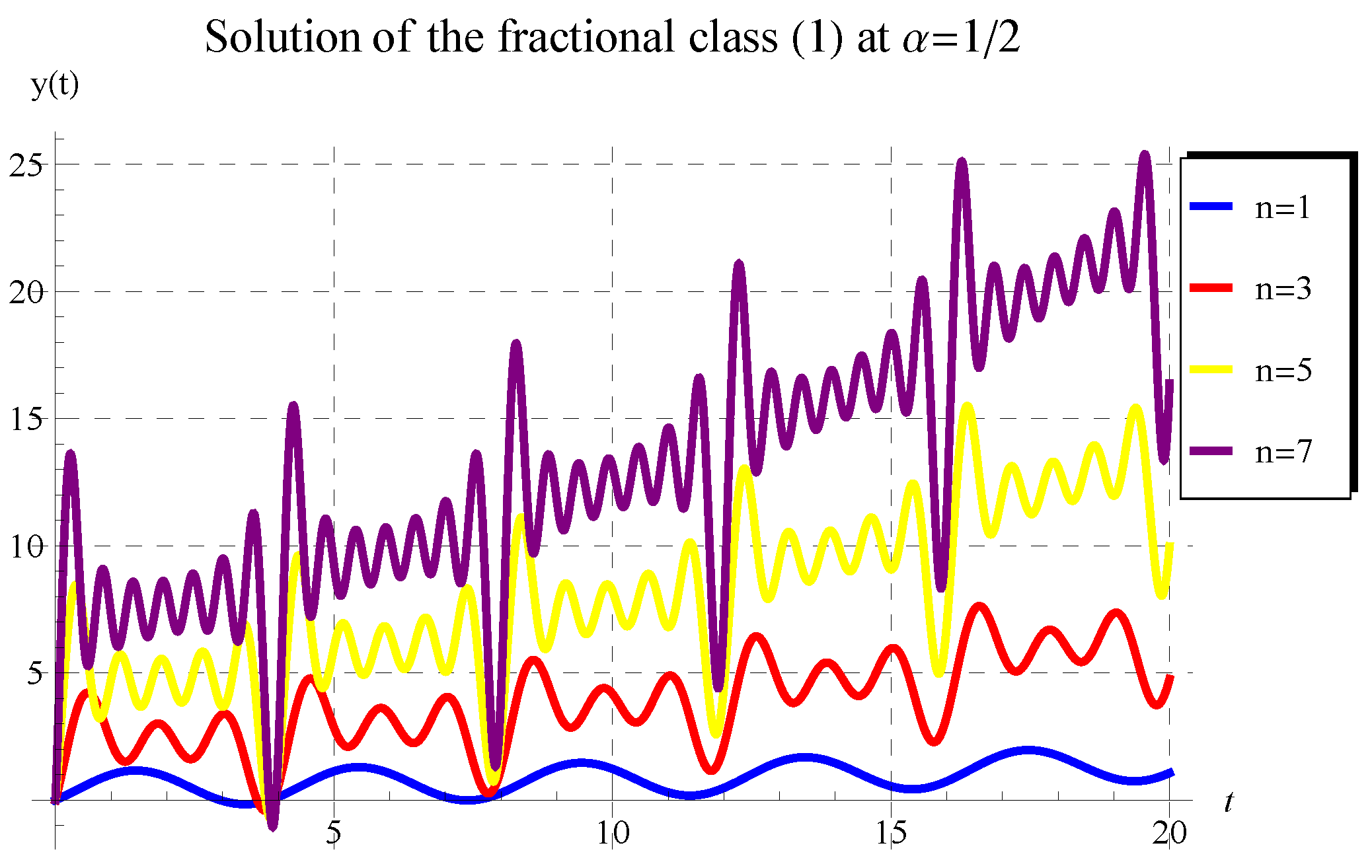
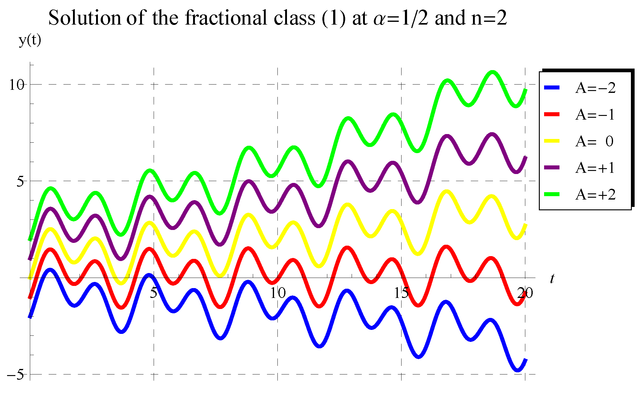
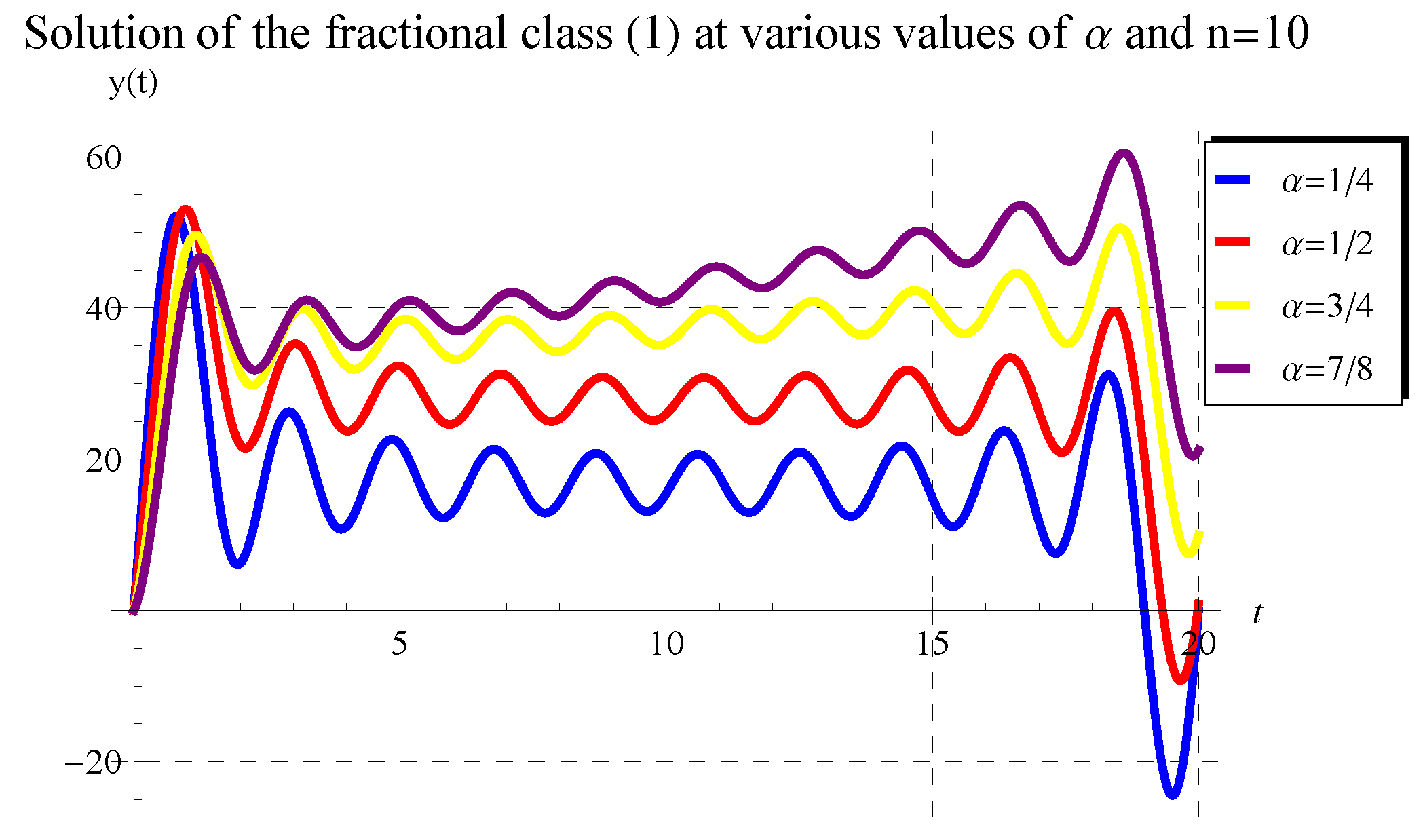
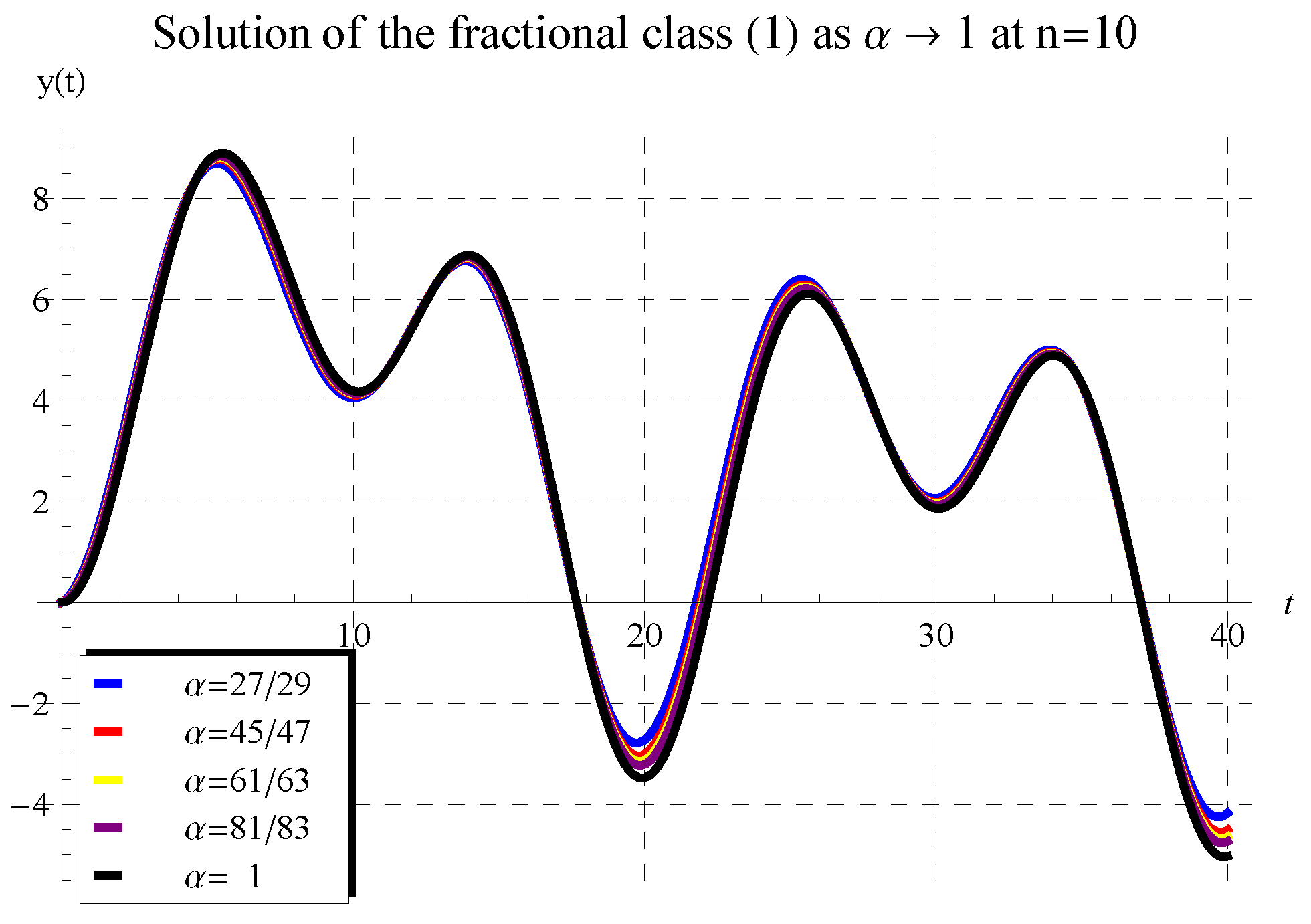
5. Behavior of Solution
6. Conclusions
Author Contributions
Funding
Data Availability Statement
Acknowledgments
Conflicts of Interest
References
- Miller, K.S.; Ross, B. An Introduction to the Fractional Calculus and Fractional Differential Equations; John Wiley & Sons: New York, NY, USA, 1993. [Google Scholar]
- Podlubny, I. Fractional Differential Equations; Academic Press: San Diego, CA, USA, 1999. [Google Scholar]
- Hilfer, R. Applications of Fractional Calculus in Physics; World Scientific Publishing Company: Singapore, 2000. [Google Scholar]
- Achar, B.N.N.; Hanneken, J.W.; Enck, T.; Clarke, T. Dynamics of the fractional oscillator. Phys. A 2001, 297, 361–367. [Google Scholar] [CrossRef]
- Sebaa, N.; Fellah, Z.E.A.; Lauriks, W.; Depollier, C. Application of fractional calculus to ultrasonic wave propagation in human cancellous bone. Signal Process. 2006, 86, 2668–2677. [Google Scholar] [CrossRef]
- Tarasov, V.E. Fractional Heisenberg equation. Phys. Lett. A 2008, 372, 2984–2988. [Google Scholar] [CrossRef] [Green Version]
- Ding, Y.; Yea, H. A fractional-order differential equation model of HIV infection of CD4+T-cells. Math. Comput. Model. 2009, 50, 386–392. [Google Scholar] [CrossRef]
- Wang, S.; Xu, M.; Li, X. Green’s function of time fractional diffusion equation and its applications in fractional quantum mechanics. Nonlinear Anal. Real World Appl. 2009, 10, 1081–1086. [Google Scholar] [CrossRef]
- Song, L.; Xu, S.; Yang, J. Dynamical models of happiness with fractional order. Commun. Nonlinear Sci. Numer. Simul. 2010, 15, 616–628. [Google Scholar] [CrossRef]
- Ebaid, A. Analysis of projectile motion in view of the fractional calculus. Appl. Math. Model. 2011, 35, 1231–1239. [Google Scholar] [CrossRef]
- Machado, J.T.; Kiryakova, V.; Mainardi, F. Recent history of fractional calculus. Commun. Nonlinear Sci. Numer. Simul. 2011, 16, 1140–1153. [Google Scholar] [CrossRef] [Green Version]
- Ebaid, A.; El-Sayed, D.M.M.; Aljoufi, M.D. Fractional calculus model for damped Mathieu equation: Approximate analytical solution. Appl. Math. Sci. 2012, 6, 4075–4080. [Google Scholar]
- Gómez-Aguilara, J.F.; Rosales-García, J.J.; Bernal-Alvarado, J.J. Fractional mechanical oscillators. Rev. Mex. De Física 2012, 58, 348–352. [Google Scholar]
- Garcia, J.J.R.; Calderon, M.G.; Ortiz, J.M.; Baleanu, D. Motion of a particle in a resisting medium using fractional calculus approach. Proc. Rom. Acad. Ser. A 2013, 14, 42–47. [Google Scholar]
- Kumar, D.; Singh, J.; Baleanu, D.; Rathore, S. Analysis of a fractional model of the Ambartsumian equation. Eur. Phys. J. Plus 2018, 133, 133–259. [Google Scholar] [CrossRef]
- Ebaid, A.; El-Zahar, E.R.; Aljohani, A.F.; Salah, B.; Krid, M.; Machado, J.T. Analysis of the two-dimensional fractional projectile motion in view of the experimental data. Nonlinear Dyn. 2019, 97, 1711–1720. [Google Scholar] [CrossRef]
- Ebaid, A.; Cattani, C.; Juhani1, A.S.A.; El-Zahar, E.R. A novel exact solution for the fractional Ambartsumian equation. Adv. Differ. Equations 2021, 2021, 88. [Google Scholar] [CrossRef]
- Kaur, D.; Agarwal, P.; Rakshit, M.; Chand, M. Fractional Calculus involving (p,q)-Mathieu Type Series. Appl. Math. Nonlinear Sci. 2020, 5, 15–34. [Google Scholar] [CrossRef]
- Agarwal, P.; Mondal, S.R.; Nisar, K.S. On fractional integration of generalized struve functions of first kind. Thai J. Math. 2020; to appear. [Google Scholar]
- Agarwal, P.; Singh, R. Modelling of transmission dynamics of Nipah virus (Niv): A fractional order approach. Phys. A Stat. Mech. Its Appl. 2020, 547, 124243. [Google Scholar] [CrossRef]
- Alderremy, A.A.; Saad, K.M.; Agarwal, P.; Aly, S.; Jain, S. Certain new models of the multi space-fractional Gardner equation. Phys. A Stat. Mech. Its Appl. 2020, 545, 123806. [Google Scholar] [CrossRef]
- Aljohani, A.F.; Ebaid, A.; Algehyne, E.A.; Mahrous, Y.M.; Cattani, C.; Al-Jeaid, H.K. The Mittag-Leffler function for re-evaluating the chlorine transport model: Comparative analysis. Fractal Fract. 2022, 6, 125. [Google Scholar] [CrossRef]
- Ahmad, B.; Batarfi, H.; Nieto, J.J.; Oscar, O.-Z.; Shammakh, W. Projectile motion via Riemann-Liouville calculus. Adv. Differ. Equ. 2015, 2015, 63. [Google Scholar] [CrossRef] [Green Version]
- Elzahar, E.R.; Gaber, A.A.; Aljohani, A.F.; Machado, J.T.; Ebaid, A. Generalized Newtonian fractional model for the vertical motion of a particle. Appl. Math. Model 2020, 88, 652–660. [Google Scholar] [CrossRef]
- El-Zahar, E.R.; Alotaibi, A.M.; Ebaid, A.; Aljohani, A.F.; Gomez Aguilar, J.F. The Riemann-Liouville fractional derivative for Ambartsumian equation. Results Phys. 2020, 19, 103551. [Google Scholar] [CrossRef]
- Ebaid, A.; Masaedeh, B.; El-Zahar, E. A new fractional model for the falling body problem. Chin. Phys. Lett. 2017, 34, 020201. [Google Scholar] [CrossRef]
- Khaled, S.M.; El-Zahar, E.R.; Ebaid, A. Solution of Ambartsumian delay differential equation with conformable derivative. Mathematics 2019, 7, 425. [Google Scholar] [CrossRef]
- Alharbi, F.M.; Baleanu, D.; Ebaid, A. Physical properties of the projectile motion using the conformable derivative. Chin. J. Phys. 2019, 58, 18–28. [Google Scholar] [CrossRef]
- Algehyne, E.A.; El-Zahar, E.R.; Alharbi, F.M.; Ebaid, A. Development of analytical solution for a generalized Ambartsumian equation. AIMS Math. 2020, 5, 249–258. [Google Scholar] [CrossRef]
- Ebaid, A.; Al-Jeaid, H.K. The Mittag–Leffler Functions for a Class of First-Order Fractional Initial Value Problems: Dual Solution via Riemann–Liouville Fractional Derivative. Fractal Fract. 2022, 6, 85. [Google Scholar] [CrossRef]
- Khaled, S.M.; Ebaid, A.; Mutairi, F.A. The exact endoscopic effect on the peristaltic flow of a nanofluid. J. Appl. Math. 2014, 2014, 367526. [Google Scholar] [CrossRef] [Green Version]
- Ebaid, A.; Sharif, M.A. Application of Laplace transform for the exact effect of a magnetic field on heat transfer of carbon-nanotubes suspended nanofluids. Z. Nature. A 2015, 70, 471–475. [Google Scholar] [CrossRef]
- Saleh, H.; Alali, E.; Ebaid, A. Medical applications for the flow of carbon-nanotubes suspended nanofluids in the presence of convective condition using Laplace transform. J. Assoc. Arab Univ. Basic Appl. Sci. 2017, 24, 206–212. [Google Scholar] [CrossRef] [Green Version]
- Ebaid, A.; Wazwaz, A.M.; Alali, E.; Masaedeh, B. Hypergeometric Series Solution to a Class of Second-Order Boundary Value Problems via Laplace Transform with Applications to Nanofuids. Commun. Theor. Phys. 2017, 67, 231. [Google Scholar] [CrossRef]
- Ebaid, A.; Alali, E.; Saleh, H. The exact solution of a class of boundary value problems with polynomial coefficients and its applications on nanofluids. J. Assoc. Arab Univ. Basi Appl. Sci. 2017, 24, 156–159. [Google Scholar] [CrossRef] [Green Version]
- Ali, H.S.; Alali, E.; Ebaid, A.; Alharbi, F.M. Analytic solution of a class of singular second-order boundary value problems with applications. Mathematics 2019, 7, 172. [Google Scholar] [CrossRef] [Green Version]
- Ebaid, A.; Alharbi, W.; Aljoufi, M.D.; El-Zahar, E.R. The exact solution of the falling body problem in three-dimensions: Comparative study. Mathematics 2020, 8, 1726. [Google Scholar] [CrossRef]
- El-Dib, Y.O.; Elgazery, N.S. Effect of Fractional Derivative Properties on the Periodic Solution of the Nonlinear Oscillations. Fractals 2020, 28, 2050095. [Google Scholar] [CrossRef]
- Azam, M. Effects of Cattaneo-Christov heat flux and nonlinear thermal radiation on MHD Maxwell nanofluid with Arrhenius activation energy. Case Stud. Therm. Eng. 2022, 34, 102048. [Google Scholar] [CrossRef]
- Azam, M. Bioconvection and nonlinear thermal extrusion in development ofchemically reactive Sutterby nano-material due to gyrotactic microorganisms. Int. Commun. Heat Mass Transf. 2022, 130, 105820. [Google Scholar] [CrossRef]
- Azam, M.; Abbas, N.; Ganesh, K.K.; Wali, S. Transient bioconvection and activation energy impacts on Casson nanofluid with gyrotactic microorganisms and nonlinear radiation. Waves Random Complex Media 2022, 1–20. [Google Scholar] [CrossRef]
- Azam, M.; Nayak, M.K.; Khan, W.A.; Khan, M. Significance of bioconvection and variable thermal properties on dissipative Maxwell nanofluid due to gyrotactic microorganisms and partial slip. Waves Random Complex Media 2022, 1–21. [Google Scholar] [CrossRef]
- Azam, M.; Xu, T.; Nayak, M.K.; Khan, W.A.; Khan, M. Gyrotactic microorganisms and viscous dissipation features on radiative Casson nanoliquid over a moving cylinder with activation energy. Waves Random Complex Media 2022, 1–23. [Google Scholar] [CrossRef]
- Oderinu, R.A.; Owolabi, J.A.; Taiwo, M. Approximate solutions of linear time-fractional differential equations. J. Math. Comput. Sci. 2022, 29, 60–72. [Google Scholar] [CrossRef]
- Akram, T.; Abbas, M.; Ali, A. A numerical study on time fractional Fisher equation using an extended cubic B-spline approximation. J. Math. Comput. Sci. 2021, 22, 85–96. [Google Scholar] [CrossRef]
- AlAhmad, R.; AlAhmad, Q.; Abdelhadi, A. Solution of fractional autonomous ordinary differential Equations. J. Math. Comput. Sci. 2022, 27, 59–64. [Google Scholar] [CrossRef]
- Nikan, O.; Avazzadeh, Z.; Machado, J.T. An efficient local meshless approach for solving nonlinear time-fractional fourth-order diffusion model. J. King Saud Univ.-Sci. 2021, 33, 101243. [Google Scholar] [CrossRef]


Publisher’s Note: MDPI stays neutral with regard to jurisdictional claims in published maps and institutional affiliations. |
© 2022 by the authors. Licensee MDPI, Basel, Switzerland. This article is an open access article distributed under the terms and conditions of the Creative Commons Attribution (CC BY) license (https://creativecommons.org/licenses/by/4.0/).
Share and Cite
Seddek, L.F.; El-Zahar, E.R.; Ebaid, A. The Exact Solutions of Fractional Differential Systems with n Sinusoidal Terms under Physical Conditions. Symmetry 2022, 14, 2539. https://doi.org/10.3390/sym14122539
Seddek LF, El-Zahar ER, Ebaid A. The Exact Solutions of Fractional Differential Systems with n Sinusoidal Terms under Physical Conditions. Symmetry. 2022; 14(12):2539. https://doi.org/10.3390/sym14122539
Chicago/Turabian StyleSeddek, Laila F., Essam R. El-Zahar, and Abdelhalim Ebaid. 2022. "The Exact Solutions of Fractional Differential Systems with n Sinusoidal Terms under Physical Conditions" Symmetry 14, no. 12: 2539. https://doi.org/10.3390/sym14122539