A Theoretical Development of Cubic Pythagorean Fuzzy Soft Set with Its Application in Multi-Attribute Decision Making

Abstract

Scientific progression has allowed researchers to develop novel and innovative ways to deal with uncertainty in data, allowing for the development of more precise and accurate data representation models. This paper aims to extend an already reported concept of Cubic Pythagorean fuzzy set to Cubic Pythagorean Fuzzy Soft Set $\left(C_{PFSs}\right)$ as it incorporates both interval-valued Pythagorean fuzzy sets (IVPFS) and Pythagorean fuzzy sets (PFS) at the same time, providing a more targeted approach to deal with uncertainty. This hybrid structure can better handle data in comparison to the ones in the literature by having the characteristics of PFS and soft sets, leading to a more targeted approach to handle attributes in decision-making studies. In this study, we defined various internals and externals of $C_{PFSs}$, set operators, aggregation operators, and developed an algorithm based on distance measures for ($C_{PFSs}$), which are applied in a disease diagnostic decision-making problem.

1. Introduction

The terms vagueness and randomness have been used over time as an element in probability theory. The terms indeterminacy and uncertainty gained significant attention around the 1960s when they were characterized using different dimensions. This allowed for the division of the concept of uncertainty into a multitude of factors; randomness, considered to be vagueness before, is now only a small part of computing the uncertainty of a system. The term vagueness nowadays refers to the deficiency or inadequacy of information in a system. These deficiencies can be technological constraints, measurement constraints, intuitionistic constraints, time-dependent variables, and functional biological variables. Finding the optimal solution to a particular problem has become better due to recent developments in information technology and decision sciences. Theoretically, facts regarding likely selections are acquired in precise quantities, but aggregated statistics tend to hide misinformation which leads to uncertain and inaccurate results. The decision maker must re-evaluate the options based on various suggestive criteria such as intervals and figures. However, due to the record’s various feedback effects, it is sometimes impossible for one individual to take action. One explanation may be a lack of knowledge or a contradiction. As a result, a series of statements are offered to consider the measurement of the indicated unfavourable features in a scientific manner. Considering these factors, in studies involving similarity measures or in mapping studies for the determination of symmetry or pattern recognition of real systems, it is essential to determine these uncertainties as these may have implications and may lead to unrealistic results when considering numerous factors at the same time. In order to put these indeterministic factors into computational and measurable boundaries, Zadeh [1] presented the idea of a fuzzy set (FS) in 1965. It deviates from classical set theory by assigning a membership degree between [0, 1] to a given element in a set.

In classical set theory, scenarios are dealt with as exact solutions, which is not ideal for most cases as some parameters are approximations that leave room for uncertainty to hinder the final solution. FS theory allows for the computation of an approximation solution. Zadeh [2] also presented the concept of interval-valued fuzzy sets (IVFS) in 1975. The FSs are based on the membership value, but some situations are still difficult to address just by using the membership function. Here, interval-valued fuzzy is preferred to determine the membership degree as the membership value is expressed in a fuzzy interval. In 2012, Y.B. JUN [3] came up with a concept of a hybrid IVFS and FS structure to develop a Cubic Set (CS) and its associated properties. Cubic sets can be applied to address the range evaluation issue of an object at a particular event in time.

Atanassov [4] defined the term intuitionistic fuzzy set (IFS) in 1986. The membership function, non-membership function, and hesitation margins are the three parameters that define IFS, whereas the membership function is the only component that defines the FS. In IFS, each element will be allocated both membership and non-membership values which are more appropriate than others. The following factors can cause these:

• Decision makers (DMs) may lack precise or sufficient information about the problem.
• DMs may be unable to explicitly discriminate the superiority of one alternative over another [5]. In such cases, DMs may provide their assessments on alternatives to a degree rather than with complete certainty [6].

Atanassov and Gargov [7] developed the concept of interval-valued intuitionistic fuzzy set (IVIFS) in 1989, which is a further development of IFS. As a result, DMs may find it more convenient to convey their judgements using IFS rather than exact numerical values or linguistic variables [8,9], particularly IVIFSs. In reality, using membership and non-membership degrees to communicate ideas allows DMs to quickly and properly represent their judgments of decision difficulties. A significant amount of research has been performed on IVIFS in the literature, with a focus on the basic theory of IVIFS, such as the relations and operations of IVIFS [10], the correlation and correlation coefficients of IVIFS [11,12], the topology of IVIFS [13], the relationships among the IVIFS, L-fuzzy set, IFS, IVFS [14], and pattern recognition [15]. Gagandeep Kaur and Harish Garg [16,17] presented the idea of a cubic intuitionistic fuzzy set (CIFS) in 2018, characterized by two parts simultaneously, one of which expresses the membership and non-membership values by an IVIFS and the other by an IFS.

After some modernization of fuzzy sets, a soft set (SS) was introduced by Molodtsov [18] in 1999. The soft set theory defines the parameters along all elements of the universal set. With the concept of fuzzy sets and soft sets, Maji et al. [19] established the notion of fuzzy soft sets (FSS) in 2001. In everyday life, people are frequently confronted with challenges that require the use of good judgment. However, in most circumstances, it becomes perplexing to define the best answer. Several solution-related parameters must be investigated to achieve the best viable solution to these issues. In 2009, X.B. Yang et al. [20] developed a hybrid of the interval-valued fuzzy soft set (IVFSS) and defined some operations. By using interval-valued fuzzy soft set and fuzzy soft set, Muhiuddin et al. [21] introduced a new notion called cubic soft set (CSS) in 2014. A structure of intuitionistic fuzzy soft sets (IFSS) [22] was proposed by Maji et al. in 2004. Yunqiang Yin et al. [23] investigated the operation features and algebraic structure of IFSS in 2012. Yuncheng Jiang et al. proposed a combination of IVFSS and IFSS in 2010 [24], which they refer to as interval-valued intuitionistic fuzzy soft set (IVIFSS).

In 2018, by changing the function into a multi-attributive function, Florentin Smarandache [25] expanded the soft set to the hypersoft set (HSS) and presented the hybrids Crisp, Fuzzy (FHSS), Intuitionistic Fuzzy (IFHSS), Neutrosophic (NHSS), and Plithogenic Hypersoft Set (PHSS). Compared to SS and other current theories, HSS is the most appropriate to address multi-attribute decision-making problems when considering the parameters’ multi-subattributes while managing to address ambiguous and uncertain information. Several HSS extensions have been developed in the literature and have been applied in decision-making. In 2021, Amarendra babu and Siva Naga Malleswari [26] defined intuitionistic fuzzy soft cubic relations and used some examples of intuitionistic fuzzy soft cubic.

Pythagorean Fuzzy Sets lack the ability to address individual parameters in a decision-making problem with multiple parameters. Its combination with soft set theory helps to address this issue. The combination of the hybrid structure with Cubic Fuzzy Set (CFS) addresses interval values and membership and non-membership values simultaneously. This hybrid model considers two different time zones used in an experiment simultaneously. To elaborate further, consider an individual performing an experiment and observations are made at two different intervals as one of the observations may have some uncertainty. Let the observations be in the uncertain range of [0.3, 0.6] at time T1; the crisp value will either agree with the interval (P-order) or disagree (R-order). This hybrid environment greatly influences the precision of the process by enhancing the scope of the interval by considering a membership value of a fuzzy nature that corresponds to the interval. A cubic Pythagorean fuzzy soft set allows for a realm of possibilities of handling complex data types and addressing a number of time-scale problems when proper operations are defined.

The structure is particularly useful when considering data where a fuzzy value in the form of a membership and non-membership value are to be simultaneously considered with the interval from which those values are extrapolated from. The soft set aspect of the structure helps to address individual parameters in a cubic Pythagorean fuzzy format which provides a more diverse and concise analysis. This structure is particularly useful when considering data present in the form of medical tests. The test results of a patient are presented in the form of membership value that needs to be in an interval for the patient to be in a healthy condition. With the distance measures developed in the manuscript, tentative testing can be performed for proof of concept, thereby making the structure applicable in this area.

The paper is divided into the following five sections: Section 2 focuses on the preliminary definitions that are used for defining the novel concept in the paper. Section 3 presents the concept of Cubic Pythagorean Fuzzy Soft Set alongside its fundamental operations. Section 4 defines different distance measures with examples for the novel structure while Section 6 presents the application of those distance measures in developing a decision-making algorithm that is used to develop a decision-support system for medical diagnostic purposes. The conclusion section presents the summary of the work alongside the future directions that can be generated from the presented work.

2. Preliminaries

This section of the paper focuses on providing some basic definitions from the literature that have been utilized for this research.

2.1. Fuzzy Set

Introduced by Zadeh [1], fuzzy set has become a necessary tool to hold errors and vagueness in different areas.

Assume $\mathsf{\Omega }$ to be a universal set. Then, the fuzzy set in $\mathsf{\Omega }$ can be initiated by the membership function ${\iota }_F$ in which every element of universal set maps with the membership function whose value lies between 0 and 1.

$$\begin{array}{c}\hfill \mathsf{\Gamma }=\left\{\langle \aleph ,{\iota }_F\left(w\right)\rangle \right|\aleph \in \mathsf{\Omega }\}\end{array}$$

$$\begin{array}{c}\hfill \mathrm{where}{\iota }_F(\aleph )\in [0,1].\end{array}$$

2.2. Interval-Valued Fuzzy Set

Zadeh [2] also developed the concept of interval-valued fuzzy sets, alongside Grattan-Guiness [27], Jahn [28], Sambuc [29], in the seventies, in the same year. An interval-valued membership function defines an interval-valued fuzzy set (IVF).

Assume $\mathsf{\Omega }$ to be a universal set. Then, the interval-valued fuzzy set can be initiated by the ${\iota }_{IVF}^I$ membership function which is the subinterval of $[0,1]$ in which every element of universal set maps with the interval-valued degree membership.

$$\begin{array}{c}\hfill \mathsf{\Lambda }=\left\{\langle \aleph ,{\iota }_{IVF}^I(\aleph )\rangle \right|\aleph \in \mathsf{\Omega }\}\end{array}$$

$$\begin{array}{c}\hfill \mathrm{where}{\iota }_{IVF}^I(\aleph )\subseteq [0,1].\end{array}$$

2.3. Cubic Set

Jun et al. [3] proposed a fascinating idea known as cubic set theory. Cubic set is the hybrid of an Interval-Valued Fuzzy Set and Fuzzy Set.

$$\begin{array}{c}\hfill A=\left\{(\aleph ,{\mathsf{\Lambda }}_F(\aleph ),{\mathsf{\Gamma }}_F(\aleph ))\right|\aleph \in \mathsf{\Omega }\},\end{array}$$

where ${\mathsf{\Lambda }}_F(\aleph )$ is the IVF and ${\mathsf{\Gamma }}_F(\aleph )$ is the FS.

2.4. Fuzzy Soft Set

By incorporating the notions of fuzzy sets [1], Maji et al. [30] proposed the concept of fuzzy soft sets. Many intriguing applications of soft set theory have been expanded on by certain researchers utilising this notion.

A pair $(\varrho ,{\mathsf{\Xi }}_1)$ is said to be fuzzy soft set over $\mathsf{\Omega }$

$$\begin{array}{c}\hfill \varrho =\left\{(\varpi ,f_{\wp }\left(\varpi \right))\right|\varpi \in {\mathsf{\Xi }}_1,f_{\wp }\left(\varpi \right)\in F\left(\mathsf{\Omega }\right)\}\end{array}$$

where

$$\begin{array}{c}\hfill f_{\wp }\left(\varpi \right)=\left\{\langle \aleph ,{\iota }_F(\aleph )\rangle \right|\aleph \in \mathsf{\Omega }\}\end{array}$$

$$\begin{array}{c}\hfill {\iota }_F(\aleph )\in [0,1]\end{array}$$

where $f_{\wp }:{\mathsf{\Xi }}_1\to F\left(\mathsf{\Omega }\right)$

2.5. Interval-Valued Fuzzy Soft Set

The extension of fuzzy soft sets was introduced by Maji et al. [30] to interval-valued fuzzy soft sets. IVFSs were created on their own to address some of the issues with fuzzy soft sets.

Suppose $\mathsf{\Omega }$ to be a universal set, $\mathsf{\Xi }$ to be an attributive set and ${\mathsf{\Xi }}_1\subseteq \mathsf{\Xi }$. Then, the pair $(\tilde{\mathsf{\Lambda }},{\mathsf{\Xi }}_1)$ is defined as an interval-valued fuzzy soft set with the mapping

$$\begin{array}{c}\hfill \tilde{\mathsf{\Lambda }}:{\mathsf{\Xi }}_1\to \tilde{P}\left(\mathsf{\Omega }\right)\end{array}$$

where $\tilde{P}\left(\mathsf{\Omega }\right)$ is the subsets of all interval-valued fuzzy elements.

A pair $(\tilde{\mathsf{\Lambda }},{\mathsf{\Xi }}_1)$ can be expressed as

$$\begin{array}{c}\hfill (\tilde{\mathsf{\Lambda }},{\mathsf{\Xi }}_1)=\left\{\langle \varpi ,f_{\wp }\left(\varpi \right)\rangle \right|\varpi \in {\mathsf{\Xi }}_1,f_{\wp }\left(\varpi \right)\in IVF\left(\mathsf{\Omega }\right)\}\end{array}$$

where

$$\begin{array}{c}\hfill f_{\wp }\left(\varpi \right)=\{\langle \aleph ,{\iota }_{IVF}^I(\aleph )|\aleph \in \mathsf{\Omega }\}\end{array}$$

and

$$\begin{array}{c}\hfill {\iota }_{IVF}^I(\aleph )\subseteq [0,1]\end{array}$$

$$\begin{array}{c}\hfill \mathrm{where} {\iota }_{IVF}^I(\aleph )=[{\iota }_{IVF}^L,{\iota }_{IVF}^U].\end{array}$$

Example 1.

Assume that $\mathsf{\Omega }=\{{\aleph }_1,{\aleph }_2,{\aleph }_3\}$ is a universal set, and $\mathsf{\Xi }=\{{\varpi }_1,{\varpi }_2,{\varpi }_3,{\varpi }_4\}$ is an attributive set with respect to Y. Let ${\mathsf{\Xi }}_1=\{{\varpi }_1,{\varpi }_2,{\varpi }_3\}\subseteq \mathsf{\Xi }$; then, an interval-valued fuzzy soft set $\tilde{\mathsf{\Lambda }}$ can be defined as

$$\begin{array}{c}\hfill \tilde{\mathsf{\Lambda }}=\{\langle {\varpi }_1,\{({\aleph }_1,[0.1,0.2]),({\aleph }_2,[0.3,0.7]),({\aleph }_3,[0.2,0.6])\}\rangle ,\end{array}$$

$$\begin{array}{c}\hfill \langle {\varpi }_2,\{({\aleph }_1,[0.2,0.6]),({\aleph }_2,[0.1,0.8]),({\aleph }_3,[0.2,0.5])\}\rangle ,\end{array}$$

$$\begin{array}{c}\hfill \langle {\varpi }_3,\{({\aleph }_1,[0.1,0.3]),({\aleph }_2,[0.3,0.6]),({\aleph }_3,[0.2,0.7])\}\rangle \}.\end{array}$$

2.6. Cubic Soft Sets

Suppose $\mathsf{\Omega }$ is a universal set, $\mathsf{\Xi }$ is an attributive set and ${\mathsf{\Xi }}_1\subseteq \mathsf{\Xi }$. Then, the cubic soft set can be expressed as

$$\begin{array}{c}\hfill C=\left\{\langle \varpi ,f_{\wp }\left(\varpi \right)\rangle \right|\varpi \in {\mathsf{\Xi }}_1,f_{\wp }\left(\varpi \right)\in C\left(\mathsf{\Omega }\right)\}\end{array}$$

where

$$\begin{array}{c}\hfill f_{\wp }\left(\varpi \right)=\left\{\langle \aleph ,({\iota }_c^I(\aleph ),{\iota }_c(\aleph ))\rangle \right|\aleph \in \mathsf{\Omega }\}\end{array}$$

where ${\iota }_c^I(\aleph )$ is interval-valued fuzzy soft set and ${\iota }_c(\aleph )$ is the fuzzy soft set with ${\iota }_c^I(\aleph )\in [0,1]$ and ${\iota }_c(\aleph )\in [0,1]$, see [21].

Example 2.

Assume that $\mathsf{\Omega }=\{{\aleph }_1,{\aleph }_2,{\aleph }_3\}$ is a universal set, and $\mathsf{\Xi }=\{{\varpi }_1,{\varpi }_2,{\varpi }_3,{\varpi }_4\}$ is an attributive set with respect to Ω. Let ${\mathsf{\Xi }}_1=\{{\varpi }_1,{\varpi }_2,{\varpi }_3\}\subseteq \mathsf{\Xi }$; then, a cubic soft set C can be defined as

$$\begin{array}{c}\hfill C=\{\langle {\varpi }_1,\{({\aleph }_1,[0.1,0.2],0.3),({\aleph }_2,[0.3,0.7],0.4),({\aleph }_3,[0.2,0.6],0.7)\}\rangle ,\end{array}$$

$$\begin{array}{c}\hfill \langle {\varpi }_2,\{({\aleph }_1,[0.2,0.6],0.4),({\aleph }_2,[0.1,0.8],0.9),({\aleph }_3,[0.2,0.5],0.3)\}\rangle ,\end{array}$$

$$\begin{array}{c}\hfill \langle {\varpi }_3,\{({\aleph }_1,[0.1,0.3],0.4),({\aleph }_2,[0.3,0.6],0.5),({\aleph }_3,[0.2,0.7],0.8)\}\rangle \}.\end{array}$$

2.7. Intuitionistic Fuzzy Set

Atanassov [4] created the Intuitionistic Fuzzy Set (IFS), which generalises the Zadeh fuzzy set [1]. Assume $\mathsf{\Omega }$ to be an universal set; then, the intuitionistic fuzzy set can be generated by the membership function ${\iota }_{\chi }(\aleph )\subseteq [0,1]$ and the non membership function ${\sigma }_{\chi }(\aleph )\subseteq [0,1]$ such as

$$\begin{array}{c}\hfill \chi =\left\{\langle \aleph ,{\iota }_{\chi }(\aleph ),{\sigma }_{\chi }(\aleph )\rangle \right|\aleph \in \mathsf{\Omega }\}\end{array}$$

where

$$\begin{array}{c}\hfill 0\le {\iota }_{\chi }(\aleph ))+{\sigma }_{\chi }(\aleph )\le 1\end{array}$$

Example 3.

Assume that $\mathsf{\Omega }=\{{\aleph }_1,{\aleph }_2,{\aleph }_3\}$ be a universal set, then the IFS χ can be written as

$$\begin{array}{c}\hfill \chi =\{\langle {\aleph }_1,(0.2,0.6)\rangle ,\langle {\aleph }_2,(0.4,0.5)\rangle ,\langle {\aleph }_3,(0.3,0.7)\rangle \}.\end{array}$$

2.8. Pythagorean Fuzzy Set

The Pythagorean fuzzy set is the extension of intuitionistic fuzzy set. However, in some problems, the sum of membership degree and non membership degree may be $\ge 1$, but the square sum is $\le 1$. So, Yager [31,32] presented the idea of a Pythagorean fuzzy set (PFS). A comparison of PFS and IFS in Figure 1.

Assume $\mathsf{\Omega }$ to be a universal set; then, the Pythagorean fuzzy set can be generated by the membership function ${\iota }_{\delta }(\aleph )\subseteq [0,1]$ and the non-membership function ${\sigma }_{\delta }(\aleph )\subseteq [0,1]$ such as

$$\begin{array}{c}\hfill \delta =\left\{\langle \aleph ,{\iota }_{\delta }(\aleph ),{\sigma }_{\delta }(\aleph )\rangle \right|\aleph \in \mathsf{\Omega }\}\end{array}$$

where

$$\begin{array}{c}\hfill 0\le {\left({\iota }_{\delta }(\aleph )\right)}^2+{\left({\sigma }_{\delta }(\aleph )\right)}^2\le 1\end{array}$$

and the degree of indeterminacy is

$$\begin{array}{c}\hfill {\pi }_{\delta }=\sqrt{1-{\left({\iota }_{\delta }(\aleph )\right)}^2+{\left({\sigma }_{\delta }(\aleph )\right)}^2}.\end{array}$$

Example 4.

Let $\mathsf{\Omega }=\{{\aleph }_1,{\aleph }_2,{\aleph }_3\}$ be a universal set; then, a Pythagorean fuzzy set δ can be written as follows:

$$\begin{array}{c}\hfill \delta =\{\langle {\aleph }_1,(0.2,0.6)\rangle ,\langle {\aleph }_2,(0.4,0.9)\rangle ,\langle {\aleph }_3,(0.3,0.7)\rangle \}\end{array}$$

2.9. Pythagorean Fuzzy Soft Set

The Pythagorean fuzzy soft set (PFSs) is a helpful expansion of the Pythagorean fuzzy set (PFS) for dealing with material that is imprecise or unclear [33]. Peng et al. [34] proposed the concept of Pythagorean fuzzy soft set by combining Ss with PFS (PFSs).

Suppose $\mathsf{\Omega }$ is a universal set, $\mathsf{\Xi }$ is an attributive set and ${\mathsf{\Xi }}_1\subseteq \mathsf{\Xi }$. Then, the pair $(\tilde{\delta },{\mathsf{\Xi }}_1)$ is called a Pythagorean fuzzy soft set, where its mapping is

$$\begin{array}{c}\hfill f_{\delta }:{\mathsf{\Xi }}_1\to {\delta }^{\mathsf{\Omega }}\end{array}$$

where ${\delta }^{\mathsf{\Omega }}$ is the Pythagorean fuzzy subsets of $\mathsf{\Omega }$. A pair $(\tilde{\delta },{\mathsf{\Xi }}_1)$ can be defined as

$$\begin{array}{c}\hfill \tilde{\delta }=\left\{\langle \varpi ,f_{\tilde{\delta }}\left(\varpi \right)\rangle \right|\varpi \in {\mathsf{\Xi }}_1,f_{\tilde{\delta }}\left(\varpi \right)\in {\delta }^{\mathsf{\Omega }}\}\end{array}$$

where

$$\begin{array}{c}\hfill f_{\tilde{\delta }}\left(\varpi \right)=\left\{(\aleph ,{\iota }_{\delta }(\aleph ),{\sigma }_{\delta }(\aleph ))\right|\aleph \in \mathsf{\Omega }\}\end{array}$$

if it satisfies

$$\begin{array}{c}\hfill 0\le {\left({\iota }_{\delta }(\aleph )\right)}^2+{\left({\sigma }_{\delta }(\aleph )\right)}^2\le 1.\end{array}$$

3. Cubic Pythagorean Fuzzy Soft Set

In this section, the cubic Pythagorean fuzzy soft set is introduced, which is a hybrid of the cubic Pythagorean fuzzy set and soft set.

Interval-Valued Pythagorean Fuzzy Soft Set

Suppose $\mathsf{\Omega }$ is a universal set; then, the interval-valued Pythagorean fuzzy soft set can be initiated by ${\iota }_{\delta }^I(\aleph )\subseteq [0,1]$, which is the membership function and ${\sigma }_{\delta }^I(\aleph )\subseteq [0,1]$ is the non-membership function.

$$\begin{array}{c}\hfill \widehat{\delta }=\left\{\langle \varpi ,f_{\tilde{\delta }}\left(\varpi \right)\rangle \right|\varpi \in {\mathsf{\Xi }}_1,f_{\tilde{\delta }}\left(\varpi \right)\in {\widehat{\delta }}^{\mathsf{\Omega }}\}\end{array}$$

where ${\widehat{\delta }}^{\mathsf{\Omega }}$ is the interval-valued Pythagorean fuzzy subset and

$$\begin{array}{c}\hfill f_{\tilde{\delta }}\left(\varpi \right)=\left\{\langle \aleph ,{\iota }_{\delta }^I(\aleph ),{\sigma }_{\delta }^I(\aleph )\rangle \right|\aleph \in \mathsf{\Omega }\}\end{array}$$

where

$$\begin{array}{c}\hfill {\iota }_{\delta }^I(\aleph )=[{\iota }_{\delta }^L(\aleph ),{\iota }_{\delta }^U(\aleph )]\end{array}$$

and

$$\begin{array}{c}\hfill {\sigma }_{\delta }^I(\aleph )=[{\sigma }_{\delta }^L(\aleph ),{\sigma }_{\delta }^U(\aleph )]\end{array}$$

$$\begin{array}{c}\hfill \mathrm{if} \mathrm{it} \mathrm{satisfies} 0\le {\left({\iota }_{\delta }^U(\aleph )\right)}^2+{\left({\sigma }_{\delta }^U(\aleph )\right)}^2\le 1\end{array}$$

and ${\pi }_{\delta }(\aleph )=[\sqrt{1-{\left({\iota }_{\delta }^L(\aleph )\right)}^2-{\left({\sigma }_{\delta }^L(\aleph )\right)}^2},\sqrt{1-{\left({\iota }_{\delta }^U(\aleph )\right)}^2-{\left({\sigma }_{\delta }^U(\aleph )\right)}^2}]$, which is called an interval-valued Pythagorean fuzzy soft number.

Example 5.

Assume $\mathsf{\Omega }=\{{\aleph }_1,{\aleph }_2,{\aleph }_3\}$ be a set of agricultural sites and $\mathsf{\Xi }=\{{\varpi }_1,{\varpi }_2,{\varpi }_3,{\varpi }_4\}$ be the expected yield of those sites. Let ${\mathsf{\Xi }}_1=\{{\varpi }_1,{\varpi }_2,{\varpi }_3\}\subseteq \mathsf{\Xi }$; $\widehat{\delta }$ can then be written as

$$\widehat{\delta }=\left\{\begin{array}{c}\langle {\varpi }_1,\{({\aleph }_1,([0.3,0.8],[0.2,0.4])),({\aleph }_2,([0.1,0.3],[0.2,0.3])),({\aleph }_3,([0.3,0.4],[0.2,0.9]))\}\rangle ,\\ \langle {\varpi }_2,\{({\aleph }_1,([0.2,0.4],[0.1,0.3])),({\aleph }_2,([0.4,0.5],[0.1,0.3])),({\aleph }_3,([0.1,0.5],[0.1,0.3]))\}\rangle ,\\ \langle {\varpi }_3,\{({\aleph }_1,([0.3,0.6],[0.2,0.5])),({\aleph }_2,([0.4,0.7],[0.2,0.6])),({\aleph }_3,([0.3,0.9],[0.4,0.6]))\}\rangle \end{array}\right\}$$

4. Cubic Pythagorean Fuzzy Soft Set

Suppose $\mathsf{\Omega }$ is a universal set, $\mathsf{\Xi }$ is an attributive set and ${\mathsf{\Xi }}_1\subseteq \mathsf{\Xi }$, then the cubic Pythagorean fuzzy soft set can be generated as follows:

$$\begin{array}{c}\hfill Ç=\left\{\langle \varpi ,f_{\tilde{\delta }}\left(\varpi \right)\rangle \right|\varpi \in {\mathsf{\Xi }}_1,f_{\tilde{\delta }}\left(\varpi \right)\in \tilde{C}\left(\mathsf{\Omega }\right)\}\end{array}$$

where $\tilde{C}\left(\mathsf{\Omega }\right)$ is the cubic Pythagorean fuzzy soft set,

$$\begin{array}{c}\hfill f_{\tilde{\delta }}\left(\varpi \right)=\left\{\langle \aleph ,({\iota }_{\tilde{c}}^I(\aleph ),{\sigma }_{\tilde{c}}^I(\aleph )),({\iota }_{\tilde{c}}(\aleph ),{\sigma }_{\tilde{c}}(\aleph ))\rangle \right|\aleph \in \mathsf{\Omega }\}\end{array}$$

where $({\iota }_{\tilde{c}}(\aleph ),{\sigma }_{\tilde{c}}(\aleph ))$ is the Pythagorean fuzzy set and $({\iota }_{\tilde{c}}^I(\aleph ),{\sigma }_{\tilde{c}}^I(\aleph ))$ is the interval-valued Pythagorean fuzzy set.

Example 6.

Assume $\mathsf{\Omega }=\{{\aleph }_1,{\aleph }_2,{\aleph }_3\}$ to be a set of agricultural sites and $\mathsf{\Xi }=\{{\varpi }_1,{\varpi }_2,{\varpi }_3,{\varpi }_4\}$ is the expected yield of those sites. Let ${\mathsf{\Xi }}_1=\{{\varpi }_1,{\varpi }_2,{\varpi }_3\}\subseteq \mathsf{\Xi }$; then, Ç can be written as

$$\begin{array}{c}Ç=\langle {\varpi }_1,\{({\aleph }_1,([0.2,0.9],[0.2,0.4]),(0.9,0.3)),({\aleph }_2,([0.1,0.3],[0.2,0.3]),(0.3,0.6)),({\aleph }_3,([0.3,0.4],[0.3,0.9]),(0.2,0.5))\}\rangle ,\\ \langle {\varpi }_2,\{({\aleph }_1,([0.2,0.4],[0.1,0.3]),(0.3,0.6)),({\aleph }_2,([0.5,0.7],[0.1,0.3]),(0.7,0.6)),({\aleph }_3,([0.1,0.5],[0.1,0.3]),(0.2,0.4))\}\rangle ,\\ \langle {\varpi }_3,\{({\aleph }_1,([0.3,0.6],[0.2,0.5]),(0.3,0.8)),({\aleph }_2,([0.4,0.5],[0.5,0.6]),(0.3,0.7)),({\aleph }_3,([0.3,0.4],[0.4,0.6]),(0.4,0.9))\}\rangle \}\end{array}$$

4.1. Positive-Internal Cubic Pythagorean Fuzzy Soft Set

Suppose $\mathsf{\Omega }$ is the universal set; then, the positive-internal of $C_{PFSs}$ in $\mathsf{\Omega }$ is said to be

$$\begin{array}{c}\hfill \mathrm{if} {\iota }_{\tilde{c}}^L(\aleph )\le {\iota }_{\tilde{c}}(\aleph )\le {\iota }_{\tilde{c}}^U(\aleph )\forall \aleph \in \mathsf{\Omega }\end{array}$$

Example 7.

Suppose $\mathsf{\Omega }=\{{\aleph }_1,{\aleph }_2,{\aleph }_3\}$ is the universal set; then, the positive-internal of the cubic Pythagorean fuzzy soft set is

$$\begin{array}{c}\hfill =\{\langle {\varpi }_1,\{({\aleph }_1,([0.2,0.9],[0.2,0.4]),(0.9,0.3)),({\aleph }_2,([0.1,0.3],[0.2,0.3]),(0.3,0.6)),({\aleph }_3,([0.1,0.4],[0.3,0.9]),(0.3,0.6))\}\rangle ,\end{array}$$

$$\begin{array}{c}\hfill \langle {\varpi }_2,\{({\aleph }_1,([0.2,0.4],[0.1,0.3]),(0.3,0.6)),({\aleph }_2,([0.5,0.7],[0.1,0.3]),(0.7,0.6)),({\aleph }_3,([0.1,0.5],[0.1,0.3]),(0.2,0.4))\}\rangle ,\end{array}$$

$$\begin{array}{c}\hfill \langle {\varpi }_3,\{({\aleph }_1,([0.3,0.6],[0.2,0.5]),(0.3,0.8)),({\aleph }_2,([0.4,0.6],[0.5,0.6]),(0.6,0.7)),({\aleph }_3,([0.3,0.4],[0.4,0.6]),(0.4,0.9))\}\rangle \}\end{array}$$

4.2. Negative-Internal of Cubic Pythagorean Fuzzy SoftSets

Suppose $\mathsf{\Omega }$ is the universal set; then, the negative-internal of $C_{PFSs}$ in $\mathsf{\Omega }$ is said to be

$$\begin{array}{c}\hfill \mathrm{if} {\sigma }_{\tilde{c}}^L(\aleph )\le {\sigma }_{\tilde{c}}(\aleph )\le {\sigma }_{\tilde{c}}^U(\aleph )\forall \aleph \in \mathsf{\Omega }\end{array}$$

Example 8.

If $\mathsf{\Omega }=\{{\aleph }_1,{\aleph }_2,{\aleph }_3\}$ is the universal set, then the negative-internal of the cubic Pythagorean fuzzy soft set is

$$\begin{array}{c}\hfill =\{\langle {\varpi }_1,\{({\aleph }_1,([0.2,0.9],[0.2,0.4]),(0.9,0.3)),({\aleph }_2,([0.1,0.3],[0.2,0.7]),(0.3,0.6)),({\aleph }_3,([0.3,0.4],[0.3,0.9]),(0.2,0.5))\}\rangle ,\end{array}$$

$$\begin{array}{c}\hfill \langle {\varpi }_2,\{({\aleph }_1,([0.2,0.4],[0.1,0.7]),(0.3,0.6)),({\aleph }_2,([0.5,0.7],[0.1,0.7]),(0.7,0.6)),({\aleph }_3,([0.1,0.5],[0.1,0.5]),(0.2,0.4))\}\rangle ,\end{array}$$

$$\begin{array}{c}\hfill \langle {\varpi }_3,\{({\aleph }_1,([0.3,0.6],[0.2,0.5]),(0.3,0.4)),({\aleph }_2,([0.4,0.5],[0.5,0.7]),(0.3,0.6)),({\aleph }_3,([0.3,0.4],[0.4,0.8]),(0.4,0.7))\}\rangle \}\end{array}$$

4.3. Internal Cubic Pythagorean Fuzzy Soft Set

If $\mathsf{\Omega }$ is the universal set, then the $C_{PFSs}$ in $\mathsf{\Omega }$ is said to be the internal cubic Pythagorean fuzzy soft set if it satisfies the properties of the positive-internal of $C_{PFSs}$ and negative-internal of $C_{PFSs}$.

Example 9.

If $\mathsf{\Omega }=\{{\aleph }_1,{\aleph }_2,{\aleph }_3\}$ is the universal set, then the internal cubic Pythagorean fuzzy soft set is

$$\begin{array}{c}\hfill Ç=\{\langle {\varpi }_1,\{({\aleph }_1,([0.2,0.5],[0.5,0.6]),(0.4,0.5)),({\aleph }_2,([0.3,0.5],[0.4,0.7]),(0.4,0.6)),({\aleph }_3,([0.1,0.3],[0.2,0.9]),(0.2,0.9))\}\rangle ,\end{array}$$

$$\begin{array}{c}\hfill \langle {\varpi }_2,\{({\aleph }_1,([0.1,0.7],[0.4,0.6]),(0.6,0.4)),({\aleph }_2,([0.5,0.8],[0.2,0.7]),(0.5,0.6)),({\aleph }_3,([0.2,0.4],[0.4,0.7]),(0.2,0.4))\}\rangle ,\end{array}$$

$$\begin{array}{c}\hfill \langle {\varpi }_3,\{({\aleph }_1,([0.2,0.6],[0.2,0.7]),(0.3,0.4)),({\aleph }_2,([0.3,0.5],[0.2,0.6]),(0.3,0.4)),({\aleph }_3,([0.1,0.6],[0.4,0.7]),(0.3,0.5))\}\rangle \end{array}$$

Theorem 1

Let the universal set be $\aleph =\varnothing$ and the pair $Ç{\alpha }_1=\langle ({\iota }^I,{\sigma }^I),(\iota ,\sigma )\rangle$ be a cubic Pythagorean fuzzy soft set in ℵ. If the pair $Ç{\alpha }_1=\langle ({\iota }^I,{\sigma }^I),(\iota ,\sigma )\rangle$ is a positive internal, then the complement $Ç{\alpha }_1^c=\langle {({\iota }^I,{\sigma }^I)}^c,{(\iota ,\sigma )}^c\rangle$ of $Ç{\alpha }_1=\langle ({\iota }^I,{\sigma }^I),(\iota ,\sigma )\rangle$ is a positive internal cubic Pythagorean fuzzy soft set in ℵ.

Proof. 

Let the pair $Ç{\alpha }_1=\langle ({\iota }^I,{\sigma }^I),(\iota ,\sigma )\rangle$ be a positive internal cubic picture fuzzy set in R. Then, by 3.2, we have ${\iota }_{\tilde{c}}^L(\aleph )\le {\iota }_{\tilde{c}}(\aleph )\le {\iota }_{\tilde{c}}^U(\aleph )$∀$\aleph \in \mathsf{\Omega }$; this implies that ∀$\aleph \in \mathsf{\Omega }$, $1-{\iota }_{\tilde{c}}^L(\aleph )\le 1-{\iota }_{\tilde{c}}(\aleph )\le 1-{\iota }_{\tilde{c}}^U(\aleph )$

Therefore, $Ç{\alpha }_1^c=\langle {({\iota }^I,{\sigma }^I)}^c,{(\iota ,\sigma )}^c\rangle$ is a positive internal cubic Pythagorean fuzzy soft set in ℵ. □

4.4. Positive-External of Cubic Pythagorean Fuzzy Soft Set

Suppose $\mathsf{\Omega }$ is the universal set; then, the positive-external of $C_{PFSs}$ in $\mathsf{\Omega }$ is said to be

$$\begin{array}{c}\hfill \mathrm{if} {\iota }_{\tilde{c}}(\aleph )\notin [{\iota }_{\tilde{c}}^L(\aleph ),{\iota }_{\tilde{c}}^U(\aleph )],\forall \aleph \in \mathsf{\Omega }\end{array}$$

Example 10.

If $\mathsf{\Omega }=\{{\aleph }_1,{\aleph }_2,{\aleph }_3\}$ is the universal set, then the positive-external of $C_{PFSs}$ is

$$\begin{array}{c}\hfill =\{\langle {\varpi }_1,\{({\aleph }_1,([0.2,0.5],[0.5,0.6]),(0.1,0.5)),({\aleph }_2,([0.3,0.5],[0.4,0.7]),(0.2,0.6)),({\aleph }_3,([0.1,0.3],[0.2,0.9]),(0.4,0.9))\}\rangle ,\end{array}$$

$$\begin{array}{c}\hfill \langle {\varpi }_2,\{({\aleph }_1,([0.1,0.7],[0.4,0.6]),(0.8,0.4)),({\aleph }_2,([0.5,0.8],[0.2,0.5]),(0.2,0.6)),({\aleph }_3,([0.2,0.4],[0.4,0.7]),(0.5,0.4))\}\rangle ,\end{array}$$

$$\begin{array}{c}\hfill \langle {\varpi }_3,\{({\aleph }_1,([0.2,0.6],[0.7,0.8]),(0.7,0.4)),({\aleph }_2,([0.3,0.5],[0.2,0.6]),(0.1,0.4)),({\aleph }_3,([0.1,0.6],[0.4,0.7]),(0.7,0.5))\}\rangle \end{array}$$

4.5. Negative-External of Cubic Pythagorean Fuzzy Soft Sets

If $\mathsf{\Omega }$ is the universal set, then the negative-internal of $C_{PFSs}$ in $\mathsf{\Omega }$ is said to be

$$\begin{array}{c}\hfill \mathrm{if} {\sigma }_{\tilde{c}}(\aleph )\notin [{\sigma }_{\tilde{c}}^L(\aleph ),{\sigma }_{\tilde{c}}^U(\aleph )],\forall \aleph \in \mathsf{\Omega }\end{array}$$

Example 11.

Suppose $\mathsf{\Omega }=\{{\aleph }_1,{\aleph }_2,{\aleph }_3\}$ is the universal set; then, the negative-external of cubic Pythagorean fuzzy soft set is

$$\begin{array}{c}\hfill =\{\langle {\varpi }_1,\{({\aleph }_1,([0.2,0.5],[0.5,0.6]),(0.4,0.7)),({\aleph }_2,([0.3,0.5],[0.4,0.7]),(0.4,0.3)),({\aleph }_3,([0.1,0.3],[0.2,0.9]),(0.2,0.1))\}\rangle ,\end{array}$$

$$\begin{array}{c}\hfill \langle {\varpi }_2,\{({\aleph }_1,([0.1,0.7],[0.4,0.6]),(0.6,0.3)),({\aleph }_2,([0.5,0.8],[0.2,0.7]),(0.5,0.1)),({\aleph }_3,([0.2,0.4],[0.4,0.7]),(0.2,0.3))\}\rangle ,\end{array}$$

$$\begin{array}{c}\hfill \langle {\varpi }_3,\{({\aleph }_1,([0.2,0.6],[0.2,0.7]),(0.3,0.1)),({\aleph }_2,([0.3,0.5],[0.2,0.6]),(0.3,0.8)),({\aleph }_3,([0.1,0.6],[0.4,0.7]),(0.3,0.9))\}\rangle ,\end{array}$$

4.6. External Cubic Pythagorean Fuzzy Soft Set

Suppose $\mathsf{\Omega }$ is the universal set; then, the $C_{PFSs}$ in $\mathsf{\Omega }$ is said to be the internal cubic Pythagorean fuzzy soft set if it satisfies the properties of positive-internal of $C_{PFSs}$ and negative-internal $C_{PFSs}$.

Example 12.

Suppose $\mathsf{\Omega }=\{{\aleph }_1,{\aleph }_2,{\aleph }_3\}$ is the universal set; then, the external cubic Pythagorean fuzzy soft set is

$$\begin{array}{c}\hfill =\{\langle {\varpi }_1,\{({\aleph }_1,([0.2,0.5],[0.5,0.6]),(0.1,0.7)),({\aleph }_2,([0.3,0.5],[0.4,0.7]),(0.2,0.3)),({\aleph }_3,([0.1,0.3],[0.2,0.9]),(0.5,0.1))\}\rangle ,\end{array}$$

$$\begin{array}{c}\hfill \langle {\varpi }_2,\{({\aleph }_1,([0.1,0.7],[0.4,0.6]),(0.8,0.3)),({\aleph }_2,([0.5,0.8],[0.2,0.7]),(0.4,0.1)),({\aleph }_3,([0.2,0.4],[0.4,0.7]),(0.5,0.3))\}\rangle ,\end{array}$$

$$\begin{array}{c}\hfill \langle {\varpi }_3,\{({\aleph }_1,([0.2,0.6],[0.2,0.7]),(0.7,0.1)),({\aleph }_2,([0.3,0.5],[0.2,0.6]),(0.2,0.8)),({\aleph }_3,([0.1,0.6],[0.4,0.7]),(0.7,0.9))\}\rangle ,\end{array}$$

4.7. Theorem

The universal set be $\aleph =\varnothing$ and the pair $Ç{\alpha }_1=\langle ({\iota }^I,{\sigma }^I),(\iota ,\sigma )\rangle$ be a cubic Pythagorean fuzzy soft set in ℵ. If the pair $Ç{\alpha }_1=\langle ({\iota }^I,{\sigma }^I),(\iota ,\sigma )\rangle$ is a positive external, then the complement $Ç{\alpha }_1^c=\langle {({\iota }^I,{\sigma }^I)}^c,{(\iota ,\sigma )}^c\rangle$ of $Ç{\alpha }_1=\langle ({\iota }^I,{\sigma }^I),(\iota ,\sigma )\rangle$ is a positive external cubic Pythagorean fuzzy soft set in ℵ.

Proof. 

Let the pair $Ç{\alpha }_1=\langle ({\iota }^I,{\sigma }^I),(\iota ,\sigma )\rangle$ be a positive external cubic picture fuzzy set in R. Then, by 3.5, we have ${\iota }_{\tilde{c}}(\aleph )\notin [{\iota }_{\tilde{c}}^L(\aleph ),{\iota }_{\tilde{c}}^U(\aleph )],$ ∀$\aleph \in \mathsf{\Omega }$; this implies that ∀$\aleph \in \mathsf{\Omega }$ $1-{\iota }_{\tilde{c}}(\aleph )\notin [1-{\iota }_{\tilde{c}}^L(\aleph ),1-{\iota }_{\tilde{c}}^U(\aleph )]$.

Therefore, $Ç{\alpha }_1^c=\langle {({\iota }^I,{\sigma }^I)}^c,{(\iota ,\sigma )}^c\rangle$ is a positive external cubic Pythagorean fuzzy soft set in ℵ. □

4.8. Set Operators on Cubic Pythagorean Fuzzy Soft Set

We introduced some set operators in the cubic Pythagorean fuzzy soft set.

Let $\mathsf{\Omega }=\{{\aleph }_1,{\aleph }_2,{\aleph }_3\}$ be a Universal set, and $\mathsf{\Xi }=\{{\varpi }_1,{\varpi }_2,{\varpi }_3,{\varpi }_4\}$ be an attributive set with respect to $\mathsf{\Omega }$. Let ${\mathsf{\Xi }}_1=\{{\varpi }_1,{\varpi }_2,{\varpi }_3\}\subseteq \mathsf{\Xi }$.

Assume there are two cubic Pythagorean fuzzy soft sets

$$\begin{array}{c}\hfill \beta {Ç}_1=\left\{\langle \varpi ,\{\aleph ,\left([{\iota }_{\tilde{c}}^I(\aleph ),{\sigma }_{\tilde{c}}^I(\aleph )]\right),({\iota }_{\tilde{c}}(\aleph ),{\sigma }_{\tilde{c}}(\aleph ))\}\rangle \right\}\end{array}$$

$$\begin{array}{c}\hfill \beta {Ç}_2=\left\{\langle \varpi ,\{\aleph ,\left([{\psi }_{\tilde{c}}^I(\aleph ),{\lambda }_{\tilde{c}}^I(\aleph )]\right),({\psi }_{\tilde{c}}(\aleph ),{\lambda }_{\tilde{c}}(\aleph ))\}\rangle \right\}\end{array}$$

$$\begin{array}{c}\hfill \beta {Ç}_1=\{\langle {\varpi }_1,\{({\aleph }_1,([0.2,0.5],[0.3,0.6]),(0.4,0.5)),({\aleph }_2,([0.3,0.5],[0.4,0.7]),(0.2,0.6)),({\aleph }_3,([0.1,0.3],[0.2,0.9]),(0.1,0.9))\}\rangle ,\end{array}$$

$$\begin{array}{c}\hfill \langle {\varpi }_2,\{({\aleph }_1,([0.1,0.5],[0.4,0.6]),(0.1,0.4)),({\aleph }_2,([0.5,0.7],[0.2,0.5]),(0.1,0.6)),({\aleph }_3,([0.2,0.4],[0.4,0.7]),(0.2,0.4))\}\rangle ,\end{array}$$

$$\begin{array}{c}\hfill \langle {\varpi }_3,\{({\aleph }_1,([0.2,0.6],[0.7,0.8]),(0.1,0.4)),({\aleph }_2,([0.3,0.5],[0.2,0.6]),(0.3,0.4)),({\aleph }_3,([0.1,0.6],[0.4,0.7]),(0.3,0.5))\}\rangle ,\end{array}$$

and

$$\begin{array}{c}\hfill \beta {Ç}_2=\{\langle {\varpi }_1,\{({\aleph }_1,([0.2,0.6],[0.2,0.4]),(0.3,0.4)),({\aleph }_2,([0.1,0.3],[0.2,0.3]),(0.3,0.6)),({\aleph }_3,([0.3,0.4],[0.2,0.5]),(0.2,0.5))\}\rangle ,\end{array}$$

$$\begin{array}{c}\hfill \langle {\varpi }_2,\{({\aleph }_1,([0.2,0.4],[0.1,0.3]),(0.3,0.6)),({\aleph }_2,([0.4,0.5],[0.1,0.3]),(0.3,0.6)),({\aleph }_3,([0.1,0.5],[0.1,0.3]),(0.2,0.4))\}\rangle ,\end{array}$$

$$\begin{array}{c}\hfill \langle {\varpi }_3,\{({\aleph }_1,([0.3,0.6],[0.2,0.5]),(0.3,0.8)),({\aleph }_2,([0.4,0.5],[0.2,0.6]),(0.3,0.7)),({\aleph }_3,([0.3,0.4],[0.4,0.6]),(0.3,0.6))\}\rangle \}\end{array}$$

4.8.1. Addition

$$\begin{array}{c}\hfill Ç{\alpha }_1+Ç{\alpha }_2=\{\langle {\varpi }_i,[{\{1-\prod _{i=1}^2(1-{\left({\iota }_i^L\right)}^2)\}}^{\frac{1}{2}},{\{1-\prod _{i=1}^2(1-{\left({\iota }_i^U\right)}^2)\}}^{\frac{1}{2}}],[\prod _{i=1}^2{\sigma }_i^L,\prod _{i=1}^2{\sigma }_i^U]\rangle ,\langle \prod _{i=1}^2{\iota }_i,{\{1-\prod _{i=1}^2(1-{\left({\sigma }_i\right)}^2)\}}^{\frac{1}{2}}\rangle \}\end{array}$$

Example 13.

$Ç{\alpha }_1+Ç{\alpha }_2=$

$\langle {\varpi }_1,\{({\aleph }_1,([0.3,0.7],[0.06,0.2]),(0.1,0.6)),({\aleph }_2,([0.3,0.6],[0.08,0.2]),(0.06,0.8)),({\aleph }_3,([0.3,0.5],[0.04,0.5]),(0.02,0.9))\}\rangle ,$

$$\begin{array}{c}\hfill \langle {\varpi }_2,\{({\aleph }_1,([0.2,0.6],[0.04,0.2]),(0.03,0.7)),({\aleph }_2,([0.6,0.8],[0.02,0.2]),(0.03,0.8)),({\aleph }_3,([0.2,0.6],[0.04,0.2]),(0.04,0.5))\}\rangle ,\end{array}$$

$$\begin{array}{c}\hfill \langle {\varpi }_3,\{({\aleph }_1,([0.4,0.8],[0.1,0.4]),(0.03,0.8)),({\aleph }_2,([0.5,0.7],[0.04,0.4]),(0.09,0.8)),({\aleph }_3,([0.3,0.7],[0.2,0.4]),(0.09,0.7))\}\rangle \}\end{array}$$

4.8.2. Multiplication

$$\begin{array}{c}\hfill Ç{\alpha }_1\times Ç{\alpha }_2=\{\langle {\varpi }_i,[\prod _{i=1}^2{\iota }_i^L,\prod _{i=1}^2{\iota }_i^U],[{\{1-\prod _{i=1}^2(1-{\left({\sigma }_i^L\right)}^2)\}}^{\frac{1}{2}},{\{1-\prod _{i=1}^2(1-{\left({\sigma }_i^U\right)}^2)\}}^{\frac{1}{2}}]\rangle ,\langle {\{1-\prod _{i=1}^2(1-{\left({\iota }_i\right)}^2)\}}^{\frac{1}{2}},\prod _{i=1}^2{\sigma }_i\rangle \}\end{array}$$

Example 14.

$Ç{\alpha }_1\times Ç{\alpha }_2=$

$\langle {\varpi }_1,\{({\aleph }_1,([0.04,0.3],[0.4,0.7]),(0.5,0.2)),({\aleph }_2,([0.03,0.2],[0.4,0.7]),(0.4,0.4)),({\aleph }_3,([0.03,0.1],[0.3,0.9]),(0.2,0.5))\}\rangle$,

$$\begin{array}{c}\hfill \langle {\varpi }_2,\{({\aleph }_1,([0.02,0.2],[0.4,0.6]),(0.3,0.2)),({\aleph }_2,([0.2,0.4],[0.2,0.6]),(0.3,0.4)),({\aleph }_3,([0.02,0.2],[0.4,0.7]),(0.3,0.2))\}\rangle ,\end{array}$$

$$\begin{array}{c}\hfill \langle {\varpi }_3,\{({\aleph }_1,([0.06,0.4],[0.7,0.9]),(0.3,0.3)),({\aleph }_2,([0.1,0.3],[0.3,0.8]),(0.4,0.3)),({\aleph }_3,([0.03,0.2],[0.5,0.8]),(0.4,0.3))\}\rangle \}\end{array}$$

4.8.3. Union

$$\begin{array}{c}\hfill \beta {Ç}_1\cup \beta {Ç}_2=\left(\left\{\langle {\varpi }_i,([max\{{\iota }_{{\tilde{c}}_1}^L,{\iota }_{{\tilde{c}}_2}^L\},min\{{\iota }_{{\tilde{c}}_1}^U,{\iota }_{{\tilde{c}}_2}^U\}],[max\{{\sigma }_{{\tilde{c}}_1}^L,{\sigma }_{{\tilde{c}}_2}^L\},min\{{\sigma }_{{\tilde{c}}_1}^U,{\sigma }_{{\tilde{c}}_2}^U\}]);(max\{{\iota }_{{\tilde{c}}_1},{\iota }_{{\tilde{c}}_2}\},min\{{\sigma }_{{\tilde{c}}_1},{\sigma }_{{\tilde{c}}_2}\})\rangle \right\}\right)\end{array}$$

Example 15.

$\beta {Ç}_1\cup \beta {Ç}_2=$

$\{\langle {\varpi }_1,\{({\aleph }_1,([0.2,0.5],[0.3,0.4]),(0.4,0.4)),({\aleph }_2,([0.3,0.3],[0.4,0.3]),(0.3,0.6)),({\aleph }_3,([0.3,0.3],[0.2,0.5]),(0.2,0.5))\}\rangle$,

$$\begin{array}{c}\hfill \langle {\varpi }_2,\{({\aleph }_1,([0.2,0.4],[0.4,0.3]),(0.3,0.4)),({\aleph }_2,([0.5,0.5],[0.2,0.3]),(0.3,0.6)),({\aleph }_3,([0.2,0.4],[0.4,0.3]),(0.2,0.4))\}\rangle ,\end{array}$$

$$\begin{array}{c}\hfill \langle {\varpi }_3,\{({\aleph }_1,([0.3,0.6],[0.7,0.5]),(0.3,0.4)),({\aleph }_2,([0.4,0.5],[0.2,0.6]),(0.3,0.4)),({\aleph }_3,([0.3,0.4],[0.4,0.6]),(0.3,0.5))\}\rangle \}\end{array}$$

4.8.4. Intersection

$$\begin{array}{c}\hfill \beta {Ç}_1\cap \beta {Ç}_2=\left(\left\{\langle {\varpi }_i,([min\{{\iota }_{{\tilde{c}}_1}^L,{\iota }_{{\tilde{c}}_2}^L\},max\{{\iota }_{{\tilde{c}}_1}^U,{\iota }_{{\tilde{c}}_2}^U\}],[min\{{\sigma }_{{\tilde{c}}_1}^L,{\sigma }_{{\tilde{c}}_2}^L\},max\{{\sigma }_{{\tilde{c}}_1}^U,{\sigma }_{{\tilde{c}}_2}^U\}]);(min\{{\iota }_{{\tilde{c}}_1},{\iota }_{{\tilde{c}}_2}\},max\{{\sigma }_{{\tilde{c}}_1},{\sigma }_{{\tilde{c}}_2}\})\rangle \right\}\right)\end{array}$$

Example 16.

$\beta {Ç}_1\cap \beta {Ç}_2=$

$\{\langle {\varpi }_1,\{({\aleph }_1,([0.2,0.6],[0.2,0.6]),(0.3,0.5)),({\aleph }_2,([0.1,0.5],[0.2,0.7]),(0.2,0.6)),({\aleph }_3,([0.1,0.4],[0.2,0.9]),(0.1,0.9))\}\rangle$,

$$\begin{array}{c}\hfill \{\langle {\varpi }_2,\{({\aleph }_1,([0.1,0.5],[0.1,0.6],(0.1,0.6)),({\aleph }_2,([0.4,0.7],[0.1,0.5]),(0.1,0.6)),({\aleph }_3,([0.1,0.5],[0.1,0.7]),(0.2,0.4))\}\rangle ,\end{array}$$

$$\begin{array}{c}\hfill \left\{\langle {\varpi }_3,\{({\aleph }_1,([0.2,0.6],[0.2,0.8]),(0.1,0.8)),({\aleph }_2,([0.3,0.5],[0.2,0.6]),(0.3,0.7)),({\aleph }_3,([0.1,0.6],[0.4,0.7]),(0.3,0.6))\}\rangle \right\}\end{array}$$

4.8.5. Direct Sum

$$\begin{array}{c}\hfill Ç{\alpha }_1\oplus Ç{\alpha }_2=\left(\left\{\langle {\varpi }_i,([\sqrt{{\left({\iota }_{{\tilde{c}}_1}^L\right)}^2+{\left({\iota }_{{\tilde{c}}_2}^L\right)}^2-{\left({\iota }_{{\tilde{c}}_1}^L\right)}^2{\left({\iota }_{{\tilde{c}}_2}^L\right)}^2},\sqrt{{\left({\iota }_{{\tilde{c}}_1}^U\right)}^2+{\left({\iota }_{{\tilde{c}}_2}^U\right)}^2-{\left({\iota }_{{\tilde{c}}_1}^U\right)}^2{\left({\iota }_{{\tilde{c}}_2}^U\right)}^2}],[{\sigma }_{{\tilde{c}}_1}^L{\sigma }_{{\tilde{c}}_2}^L,{\sigma }_{{\tilde{c}}_1}^U{\sigma }_{{\tilde{c}}_2}^U]);(\sqrt{{\iota }_{{\tilde{c}}_1}^2+{\iota }_{{\tilde{c}}_2}^2-{\iota }_{{\tilde{c}}_1}^2{\iota }_{{\tilde{c}}_2}^2},{\sigma }_{{\tilde{c}}_1}{\sigma }_{{\tilde{c}}_2})\rangle \right\}\right)\end{array}$$

Example 17.

$Ç{\alpha }_1\oplus Ç{\alpha }_2=$

$\{\langle {\varpi }_1,\{({\aleph }_1,([0.3,0.7],[0.06,0.2]),(0.5,0.2)),({\aleph }_2,([0.3,0.6],[0.08,0.2]),(0.6,0.4)),({\aleph }_3,([0.3,0.5],[0.04,0.5]),(0.2,0.5))\}\rangle$,

$$\begin{array}{c}\hfill \{\langle {\varpi }_2,\{({\aleph }_1,([0.2,0.6],[0.04,0.2]),(0.3,0.2)),({\aleph }_2,([0.6,0.8],[0.02,0.2]),(0.3,0.4)),({\aleph }_3,([0.2,0.6],[0.04,0.2]),(0.3,0.2))\}\rangle ,\end{array}$$

$$\begin{array}{c}\hfill \left\{\langle {\varpi }_3,\{({\aleph }_1,([0.4,0.8],[0.1,0.4]),(0.3,0.3)),({\aleph }_2,([0.5,0.8],[0.04,0.4]),(0.4,0.3)),({\aleph }_3,([0.3,0.7],[0.2,0.4]),(0.4,0.3))\}\rangle \right\}\end{array}$$

4.8.6. Direct Product

$$\begin{array}{c}\hfill Ç{\alpha }_1\otimes Ç{\alpha }_2=\left(\left\{\langle {\varpi }_i,([{\iota }_{{\tilde{c}}_1}^L{\iota }_{{\tilde{c}}_2}^L,{\iota }_{{\tilde{c}}_1}^U{\iota }_{{\tilde{c}}_2}^U],[\sqrt{{\left({\sigma }_{{\tilde{c}}_1}^L\right)}^2+{\left({\sigma }_{{\tilde{c}}_2}^L\right)}^2-{\left({\sigma }_{{\tilde{c}}_1}^L\right)}^2{\left({\sigma }_{{\tilde{c}}_2}^L\right)}^2},\sqrt{{\left({\sigma }_{{\tilde{c}}_1}^U\right)}^2+{\left({\sigma }_{{\tilde{c}}_2}^U\right)}^2-{\left({\sigma }_{{\tilde{c}}_1}^U\right)}^2{\left({\sigma }_{{\tilde{c}}_2}^U\right)}^2}]);({\iota }_{{\tilde{c}}_1}{\iota }_{{\tilde{c}}_2},\sqrt{{\sigma }_{{\tilde{c}}_1}^2+{\sigma }_{{\tilde{c}}_2}^2-{\sigma }_{{\tilde{c}}_1}^2{\sigma }_{{\tilde{c}}_2}^2})\rangle \right\}\right)\end{array}$$

Example 18.

$Ç{\alpha }_1\otimes Ç{\alpha }_2=$

$\{\langle {\varpi }_1,\{({\aleph }_1,([0.04,0.3],[0.4,0.7]),(0.1,0.6)),({\aleph }_2,([0.03,0.2],[0.4,0.7]),(0.06,0.8)),({\aleph }_3,([0.03,0.1],[0.3,0.9]),(0.02,0.9))\}\rangle$,

$$\begin{array}{c}\hfill \{\langle {\varpi }_2,({\aleph }_1,([0.02,0.2],[0.4,0.6]),(0.03,0.7)),({\aleph }_2,([0.2,0.4],[0.2,0.6]),(0.03,0.8)),({\aleph }_3,([0.02,0.2],[0.4,0.7]),(0.04,0.5))\}\rangle ,\end{array}$$

$$\begin{array}{c}\hfill \{\langle {\varpi }_3,({\aleph }_1,([0.06,0.4],[0.7,0.9]),(0.03,0.8)),({\aleph }_2,([0.1,0.3],[0.3,0.8]),(0.09,0.5)),({\aleph }_3,([0.03,0.2],[0.5,0.8]),(0.09,0.7))\}\rangle \}\end{array}$$

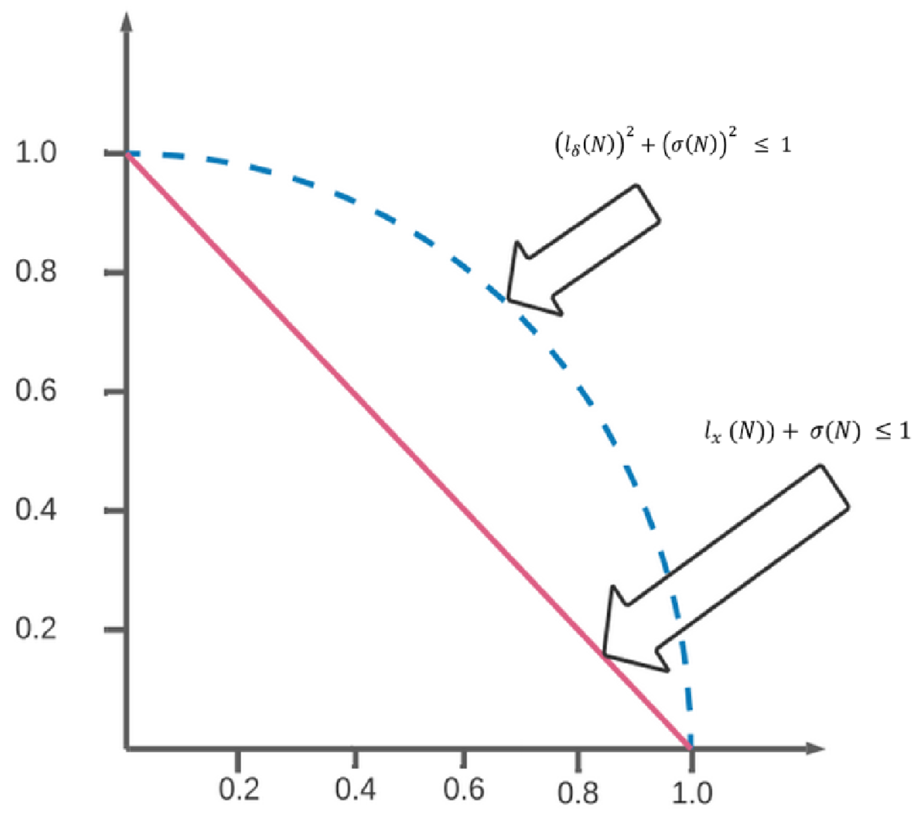
5. Distance Measures

Assume $Ç(\aleph )$ is the family of $C_{PFSs}$, which is defined using ℵ.

Definition 1.

$C_{PFSs}$$Ç{\alpha }_1,Ç{\alpha }_2$ and ${Ç}_3$; the distance measure is a real-valued function $d:Ç(\aleph )\times Ç(\aleph )\to [0,1]$ satisfying the following properties

1. 

$0\le d(Ç{\alpha }_1,Ç{\alpha }_2)\le 1;$

2. 

$d(Ç{\alpha }_1,Ç{\alpha }_2)=0$ if and only if $Ç{\alpha }_1=Ç{\alpha }_2;$

3. 

$d(Ç{\alpha }_1,Ç{\alpha }_2)=d(Ç{\alpha }_2,Ç{\alpha }_1);$

4. 

If $Ç{\alpha }_1\subseteq Ç{\alpha }_2\subseteq {Ç}_3$, then $d(Ç{\alpha }_1,Ç{\alpha }_2)\le d(Ç{\alpha }_1,{Ç}_3)$ and $d(Ç{\alpha }_2,{Ç}_3)\le d(Ç{\alpha }_1,{Ç}_3)$.

The distance measures for the $C_{PFSs}$ is defined as

$$d_q^G(Ç{\alpha }_1,Ç{\alpha }_2)={\left\{\begin{array}{c}\frac{1}{6m}{\displaystyle \sum _{i=1}^m}{\displaystyle \sum _{j=1}^n}|F_1\left({\varpi }_i\right){\left({\iota }_{Ç{\alpha }_1}^L\left({\aleph }_j\right)\right)}^2-F_2\left({\varpi }_i\right){\left({\iota }_{Ç{\alpha }_2}^L\left({\aleph }_j\right)\right)}^2{|}^q+|F_1\left({\varpi }_i\right){\left({\iota }_{Ç{\alpha }_1}^U\left({\aleph }_j\right)\right)}^2-F_2\left({\varpi }_i\right){\left({\iota }_{Ç{\alpha }_2}^U\left({\aleph }_j\right)\right)}^2{|}^q+\\ |F_1\left({\varpi }_i\right){\left({\sigma }_{Ç{\alpha }_1}^L\left({\aleph }_j\right)\right)}^2-F_2\left({\varpi }_i\right){\left({\sigma }_{Ç{\alpha }_2}^L\left({\aleph }_j\right)\right)}^2{|}^q+|F_1\left({\varpi }_i\right){\left({\sigma }_{Ç{\alpha }_1}^U\left({\aleph }_j\right)\right)}^2-F_2\left({\varpi }_i\right){\left({\sigma }_{Ç{\alpha }_2}^U\left({\aleph }_j\right)\right)}^2{|}^q+\\ |F_1\left({\varpi }_i\right){\left({\iota }_{Ç{\alpha }_1}\left({\aleph }_j\right)\right)}^2-F_2\left({\varpi }_i\right){\left({\iota }_{Ç{\alpha }_2}\left({\aleph }_j\right)\right)}^2{|}^q+|F_1\left({\varpi }_i\right){\left({\sigma }_{Ç{\alpha }_1}\left({\aleph }_j\right)\right)}^2-F_2\left({\varpi }_i\right){\left({\sigma }_{Ç{\alpha }_2}\left({\aleph }_j\right)\right)}^2{|}^q\end{array}\right\}}^{\frac{1}{q}}$$

and

$$d_q^{GN}(Ç{\alpha }_1,Ç{\alpha }_2)={\left\{\begin{array}{c}\frac{1}{6mn}{\displaystyle \sum _{i=1}^m}{\displaystyle \sum _{j=1}^n}|F_1\left({\varpi }_i\right){\left({\iota }_{Ç{\alpha }_1}^L\left({\aleph }_j\right)\right)}^2-F_2\left({\varpi }_i\right){\left({\iota }_{Ç{\alpha }_2}^L\left({\aleph }_j\right)\right)}^2{|}^q+|F_1\left({\varpi }_i\right){\left({\iota }_{Ç{\alpha }_1}^U\left({\aleph }_j\right)\right)}^2-F_2\left({\varpi }_i\right){\left({\iota }_{Ç{\alpha }_2}^U\left({\aleph }_j\right)\right)}^2{|}^q+\\ |F_1\left({\varpi }_i\right){\left({\sigma }_{Ç{\alpha }_1}^L\left({\aleph }_j\right)\right)}^2-F_2\left({\varpi }_i\right){\left({\sigma }_{Ç{\alpha }_2}^L\left({\aleph }_j\right)\right)}^2{|}^q+|F_1\left({\varpi }_i\right){\left({\sigma }_{Ç{\alpha }_1}^U\left({\aleph }_j\right)\right)}^2-F_2\left({\varpi }_i\right){\left({\sigma }_{Ç{\alpha }_2}^U\left({\aleph }_j\right)\right)}^2{|}^q+\\ |F_1\left({\varpi }_i\right){\left({\iota }_{Ç{\alpha }_1}\left({\aleph }_j\right)\right)}^2-F_2\left({\varpi }_i\right){\left({\iota }_{Ç{\alpha }_2}\left({\aleph }_j\right)\right)}^2{|}^q+|F_1\left({\varpi }_i\right){\left({\sigma }_{Ç{\alpha }_1}\left({\aleph }_j\right)\right)}^2-F_2\left({\varpi }_i\right){\left({\sigma }_{Ç{\alpha }_2}\left({\aleph }_j\right)\right)}^2{|}^q\end{array}\right\}}^{\frac{1}{q}}$$

Assume that the weight of the element is $w_i(i=1,2,3,\dots ,n)$, where $0\le w_i\le 1$ and ${\displaystyle \sum _{i=1}^n}{\left(w_i\right)}^2=1$; then, we define the generalised weight distance measure between $C_{PFSs}$ $Ç{\alpha }_1$ and $Ç{\alpha }_2$ as follows:

$$d_q^{GW}(Ç{\alpha }_1,Ç{\alpha }_2)={\left\{\begin{array}{c}\frac{1}{6m}{\displaystyle \sum _{i=1}^m}{\displaystyle \sum _{j=1}^n}{\left(w_i\right)}^2\left\{\begin{array}{c}|F_1\left({\varpi }_i\right){\left({\iota }_{Ç{\alpha }_1}^L\left({\aleph }_j\right)\right)}^2-F_2\left({\varpi }_i\right){\left({\iota }_{Ç{\alpha }_2}^L\left({\aleph }_j\right)\right)}^2{|}^q+|F_1\left({\varpi }_i\right){\left({\iota }_{Ç{\alpha }_1}^U\left({\aleph }_j\right)\right)}^2-F_2\left({\varpi }_i\right){\left({\iota }_{Ç{\alpha }_2}^U\left({\aleph }_j\right)\right)}^2{|}^q+\\ |F_1\left({\varpi }_i\right){\left({\sigma }_{Ç{\alpha }_1}^L\left({\aleph }_j\right)\right)}^2-F_2\left({\varpi }_i\right){\left({\sigma }_{Ç{\alpha }_2}^L\left({\aleph }_j\right)\right)}^2{|}^q+|F_1\left({\varpi }_i\right){\left({\sigma }_{Ç{\alpha }_1}^U\left({\aleph }_j\right)\right)}^2-F_2\left({\varpi }_i\right){\left({\sigma }_{Ç{\alpha }_2}^U\left({\aleph }_j\right)\right)}^2{|}^q+\\ |F_1\left({\varpi }_i\right){\left({\iota }_{Ç{\alpha }_1}\left({\aleph }_j\right)\right)}^2-F_2\left({\varpi }_i\right){\left({\iota }_{Ç{\alpha }_2}\left({\aleph }_j\right)\right)}^2{|}^q+|F_1\left({\varpi }_i\right){\left({\sigma }_{Ç{\alpha }_1}\left({\aleph }_j\right)\right)}^2-F_2\left({\varpi }_i\right){\left({\sigma }_{Ç{\alpha }_2}\left({\aleph }_j\right)\right)}^2{|}^q\end{array}\right\}\end{array}\right\}}^{\frac{1}{q}}$$

we also define the generalised Hausdorff distance measure for two $C_{PFSs}$ of $Ç{\alpha }_1$ and $Ç{\alpha }_2$ as follows:

$$d_q^{GW}(Ç{\alpha }_1,Ç{\alpha }_2)={\left\{\begin{array}{c}\frac{1}{6}{\displaystyle \sum _{i=1}^m}{\displaystyle \sum _{j=1}^n}max\left\{\begin{array}{c}|F_1\left({\varpi }_i\right){\left({\iota }_{Ç{\alpha }_1}^L\left({\aleph }_j\right)\right)}^2-F_2\left({\varpi }_i\right){\left({\iota }_{Ç{\alpha }_2}^L\left({\aleph }_j\right)\right)}^2{|}^q,|F_1\left({\varpi }_i\right){\left({\iota }_{Ç{\alpha }_1}^U\left({\aleph }_j\right)\right)}^2-F_2\left({\varpi }_i\right){\left({\iota }_{Ç{\alpha }_2}^U\left({\aleph }_j\right)\right)}^2{|}^q+\\ |F_1\left({\varpi }_i\right){\left({\sigma }_{Ç{\alpha }_1}^L\left({\aleph }_j\right)\right)}^2-F_2\left({\varpi }_i\right){\left({\sigma }_{Ç{\alpha }_2}^L\left({\aleph }_j\right)\right)}^2{|}^q,|F_1\left({\varpi }_i\right){\left({\sigma }_{Ç{\alpha }_1}^U\left({\aleph }_j\right)\right)}^2-F_2\left({\varpi }_i\right){\left({\sigma }_{Ç{\alpha }_2}^U\left({\aleph }_j\right)\right)}^2{|}^q+\\ |F_1\left({\varpi }_i\right){\left({\iota }_{Ç{\alpha }_1}\left({\aleph }_j\right)\right)}^2-F_2\left({\varpi }_i\right){\left({\iota }_{Ç{\alpha }_2}\left({\aleph }_j\right)\right)}^2{|}^q,|F_1\left({\varpi }_i\right){\left({\sigma }_{Ç{\alpha }_1}\left({\aleph }_j\right)\right)}^2-F_2\left({\varpi }_i\right){\left({\sigma }_{Ç{\alpha }_2}\left({\aleph }_j\right)\right)}^2{|}^q\end{array}\right\}\end{array}\right\}}^{\frac{1}{q}}$$

For $q=1$, we have the following distance measures:

1. Hamming Distance

$$d_1^G(Ç{\alpha }_1,Ç{\alpha }_2)=\frac{1}{6m}{\displaystyle \sum _{i=1}^m}{\displaystyle \sum _{j=1}^n}\left\{\begin{array}{c}|F_1\left({\varpi }_i\right){\left({\iota }_{Ç{\alpha }_1}^L\left({\aleph }_j\right)\right)}^2-F_2\left({\varpi }_i\right){\left({\iota }_{Ç{\alpha }_2}^L\left({\aleph }_j\right)\right)}^2|+|F_1\left({\varpi }_i\right){\left({\iota }_{Ç{\alpha }_1}^U\left({\aleph }_j\right)\right)}^2-F_2\left({\varpi }_i\right){\left({\iota }_{Ç{\alpha }_2}^U\left({\aleph }_j\right)\right)}^2|+\\ |F_1\left({\varpi }_i\right){\left({\sigma }_{Ç{\alpha }_1}^L\left({\aleph }_j\right)\right)}^2-F_2\left({\varpi }_i\right){\left({\sigma }_{Ç{\alpha }_2}^L\left({\aleph }_j\right)\right)}^2|+|F_1\left({\varpi }_i\right){\left({\sigma }_{Ç{\alpha }_1}^U\left({\aleph }_j\right)\right)}^2-F_2\left({\varpi }_i\right){\left({\sigma }_{Ç{\alpha }_2}^U\left({\aleph }_j\right)\right)}^2|+\\ |F_1\left({\varpi }_i\right){\left({\iota }_{Ç{\alpha }_1}\left({\aleph }_j\right)\right)}^2-F_2\left({\varpi }_i\right){\left({\iota }_{Ç{\alpha }_2}\left({\aleph }_j\right)\right)}^2|+|F_1\left({\varpi }_i\right){\left({\sigma }_{Ç{\alpha }_1}\left({\aleph }_j\right)\right)}^2-F_2\left({\varpi }_i\right){\left({\sigma }_{Ç{\alpha }_2}\left({\aleph }_j\right)\right)}^2|\end{array}\right\}$$

2. Normalised Hamming Distance

$$d_1^{GN}(Ç{\alpha }_1,Ç{\alpha }_2)=\frac{1}{6mn}{\displaystyle \sum _{i=1}^m}{\displaystyle \sum _{j=1}^n}\left\{\begin{array}{c}|F_1\left({\varpi }_i\right){\left({\iota }_{Ç{\alpha }_1}^L\left({\aleph }_j\right)\right)}^2-F_2\left({\varpi }_i\right){\left({\iota }_{Ç{\alpha }_2}^L\left({\aleph }_j\right)\right)}^2|+|F_1\left({\varpi }_i\right){\left({\iota }_{Ç{\alpha }_1}^U\left({\aleph }_j\right)\right)}^2-F_2\left({\varpi }_i\right){\left({\iota }_{Ç{\alpha }_2}^U\left({\aleph }_j\right)\right)}^2|+\\ |F_1\left({\varpi }_i\right){\left({\sigma }_{Ç{\alpha }_1}^L\left({\aleph }_j\right)\right)}^2-F_2\left({\varpi }_i\right){\left({\sigma }_{Ç{\alpha }_2}^L\left({\aleph }_j\right)\right)}^2|+|F_1\left({\varpi }_i\right){\left({\sigma }_{Ç{\alpha }_1}^U\left({\aleph }_j\right)\right)}^2-F_2\left({\varpi }_i\right){\left({\sigma }_{Ç{\alpha }_2}^U\left({\aleph }_j\right)\right)}^2|+\\ |F_1\left({\varpi }_i\right){\left({\iota }_{Ç{\alpha }_1}\left({\aleph }_j\right)\right)}^2-F_2\left({\varpi }_i\right){\left({\iota }_{Ç{\alpha }_2}\left({\aleph }_j\right)\right)}^2|+|F_1\left({\varpi }_i\right){\left({\sigma }_{Ç{\alpha }_1}\left({\aleph }_j\right)\right)}^2-F_2\left({\varpi }_i\right){\left({\sigma }_{Ç{\alpha }_2}\left({\aleph }_j\right)\right)}^2|\end{array}\right\}$$

3. Weighted Hamming Distance

$$d_1^G(Ç{\alpha }_1,Ç{\alpha }_2)=\frac{1}{6m}{\displaystyle \sum _{i=1}^m}{\displaystyle \sum _{j=1}^n}{\left(w_i\right)}^2\left\{\begin{array}{c}|F_1\left({\varpi }_i\right){\left({\iota }_{Ç{\alpha }_1}^L\left({\aleph }_j\right)\right)}^2-F_2\left({\varpi }_i\right){\left({\iota }_{Ç{\alpha }_2}^L\left({\aleph }_j\right)\right)}^2|+|F_1\left({\varpi }_i\right){\left({\iota }_{Ç{\alpha }_1}^U\left({\aleph }_j\right)\right)}^2-F_2\left({\varpi }_i\right){\left({\iota }_{Ç{\alpha }_2}^U\left({\aleph }_j\right)\right)}^2|+\\ |F_1\left({\varpi }_i\right){\left({\sigma }_{Ç{\alpha }_1}^L\left({\aleph }_j\right)\right)}^2-F_2\left({\varpi }_i\right){\left({\sigma }_{Ç{\alpha }_2}^L\left({\aleph }_j\right)\right)}^2|+|F_1\left({\varpi }_i\right){\left({\sigma }_{Ç{\alpha }_1}^U\left({\aleph }_j\right)\right)}^2-F_2\left({\varpi }_i\right){\left({\sigma }_{Ç{\alpha }_2}^U\left({\aleph }_j\right)\right)}^2|+\\ |F_1\left({\varpi }_i\right){\left({\iota }_{Ç{\alpha }_1}\left({\aleph }_j\right)\right)}^2-F_2\left({\varpi }_i\right){\left({\iota }_{Ç{\alpha }_2}\left({\aleph }_j\right)\right)}^2|+|F_1\left({\varpi }_i\right){\left({\sigma }_{Ç{\alpha }_1}\left({\aleph }_j\right)\right)}^2-F_2\left({\varpi }_i\right){\left({\sigma }_{Ç{\alpha }_2}\left({\aleph }_j\right)\right)}^2|\end{array}\right\}$$

4. Hausdorff Hamming distance

$$d_1^H(Ç{\alpha }_1,Ç{\alpha }_2)=\left\{\begin{array}{c}\frac{1}{6m}{\displaystyle \sum _{i=1}^m}{\displaystyle \sum _{j=1}^n}max\left\{\begin{array}{c}|F_1\left({\varpi }_i\right){\left({\iota }_{Ç{\alpha }_1}^L\left({\aleph }_j\right)\right)}^2-F_2\left({\varpi }_i\right){\left({\iota }_{Ç{\alpha }_2}^L\left({\aleph }_j\right)\right)}^2|,|F_1\left({\varpi }_i\right){\left({\iota }_{Ç{\alpha }_1}^U\left({\aleph }_j\right)\right)}^2-F_2\left({\varpi }_i\right){\left({\iota }_{Ç{\alpha }_2}^U\left({\aleph }_j\right)\right)}^2|,\\ |F_1\left({\varpi }_i\right){\left({\sigma }_{Ç{\alpha }_1}^L\left({\aleph }_j\right)\right)}^2-F_2\left({\varpi }_i\right){\left({\sigma }_{Ç{\alpha }_2}^L\left({\aleph }_j\right)\right)}^2|,|F_1\left({\varpi }_i\right){\left({\sigma }_{Ç{\alpha }_1}^U\left({\aleph }_j\right)\right)}^2-F_2\left({\varpi }_i\right){\left({\sigma }_{Ç{\alpha }_2}^U\left({\aleph }_j\right)\right)}^2|,\\ |F_1\left({\varpi }_i\right){\left({\iota }_{Ç{\alpha }_1}\left({\aleph }_j\right)\right)}^2-F_2\left({\varpi }_i\right){\left({\iota }_{Ç{\alpha }_2}\left({\aleph }_j\right)\right)}^2|,|F_1\left({\varpi }_i\right){\left({\sigma }_{Ç{\alpha }_1}\left({\aleph }_j\right)\right)}^2-F_2\left({\varpi }_i\right){\left({\sigma }_{Ç{\alpha }_2}\left({\aleph }_j\right)\right)}^2|\end{array}\right\}\end{array}\right\}$$

Here, we define some examples:

Assume that there are three $C_{PFSs}$

$$\begin{array}{c}\hfill \beta {Ç}_1=\{\langle {\varpi }_1,\{({\aleph }_1,([0.2,0.5],[0.2,0.8]),(0.6,0.4)),({\aleph }_2,([0.3,0.5],[0.1,0.7]),(0.9,0.3)),({\aleph }_3,([0.1,0.3],[0.2,0.9]),(0.9,0.2))\}\rangle ,\end{array}$$

$$\begin{array}{c}\hfill \langle {\varpi }_2,\{({\aleph }_1,([0.1,0.3],[0.1,0.9]),(0.4,0.4)),({\aleph }_2,([0.5,0.6],[0.2,0.8]),(0.7,0.6)),({\aleph }_3,([0.2,0.4],[0.2,0.8]),(0.5,0.6))\}\rangle ,\end{array}$$

$$\begin{array}{c}\hfill \langle {\varpi }_3,\{({\aleph }_1,([0.2,0.3],[0.1,0.8]),(0.7,0.4)),({\aleph }_2,([0.3,0.5],[0.1,0.8]),(0.8,0.4)),({\aleph }_3,([0.1,0.2],[0.1,0.9]),(0.8,0.5))\}\rangle ,\end{array}$$

and

$$\begin{array}{c}\hfill \beta {Ç}_2=\{\langle {\varpi }_1,\{({\aleph }_1,([0.2,0.6],[0.3,0.7]),(0.5,0.6)),({\aleph }_2,([0.3,0.6],[0.2,0.7]),(0.9,0.7)),({\aleph }_3,([0.4,0.5],[0.2,0.7]),(0.8,0.5))\}\rangle ,\end{array}$$

$$\begin{array}{c}\hfill \langle {\varpi }_2,\{({\aleph }_1,([0.1,0.6],[0.1,0.8]),(0.3,0.4)),({\aleph }_2,([0.2,0.5],[0.2,0.6]),(0.7,0.6)),({\aleph }_3,([0.1,0.4],[0.2,0.7]),(0.4,0.6))\}\rangle ,\end{array}$$

$$\begin{array}{c}\hfill \langle {\varpi }_3,\{({\aleph }_1,([0.2,0.4],[0.1,0.7]),(0.6,0.7)),({\aleph }_2,([0.3,0.5],[0.2,0.8]),(0.7,0.5)),({\aleph }_3,([0.1,0.5],[0.1,0.8]),(0.4,0.5))\}\rangle \}\end{array}$$

Example 19.

The hamming distance for $C_{PFSs}$ is

$$d_1^G(Ç{\alpha }_1,Ç{\alpha }_2)=\frac{1}{18}\left[\begin{array}{c}0.11+0.05+0.15+0.11+0.2+0.11+0.03+0.4+0.15+0.16+0.32+0.17+0.21+0.27+\\ \\ 0.17+0.07+0.21+0.11+0.28+0.03+0.15+0.09+0.07+0.15+0.15+0.13+0.33+\\ \\ 0.03+0.15+0.09+0.07+0.15+0.13+0.33+0.03+0.15+0.09+0.21+0.17+0.48\end{array}\right]$$

$$\begin{array}{c}\hfill =0.298\end{array}$$

Example 20.

The normalised hamming distance for $C_{PFSs}$ is

$$d_1^{GN}(Ç{\alpha }_1,Ç{\alpha }_2)=\frac{1}{54}\left[\begin{array}{c}0.11+0.05+0.15+0.11+0.2+0.11+0.03+0.4+0.15+0.16+0.32+0.17+0.21+\\ \\ 0.27+0.17+0.07+0.21+0.11+0.28+0.03+0.15+0.09+0.07+0.15+0.15+0.13+\\ \\ 0.33+0.03+0.15+0.09+0.07+0.15+0.13+0.33+0.03+0.15+0.09+0.21+0.17+0.48\end{array}\right]$$

$$\begin{array}{c}\hfill =0.09926\end{array}$$

Example 21.

The weighted hamming distance for $C_{PFSs}$ in which $w_1=0.2$, $w_2=0.3$ and $w_3=0.93$

$$\begin{array}{c}\hfill d_1^G(Ç{\alpha }_1,Ç{\alpha }_2)=\frac{1}{18}\left[\begin{array}{c}{\left(0.2\right)}^2(0.11+0.05+0.15+0.11+0.2++0.11+0.03+0.4+0.15+0.16+0.32+0.17+0.21)+\\ \\ {\left(0.3\right)}^2(0.27+0.17+0.07+0.21+0.11+0.28+0.03+0.15+0.09)+\\ \\ {\left(0.93\right)}^2(0.07+0.15+0.13+0.33+0.03+0.15+0.09+0.21+0.17+0.48)\end{array}\right]\end{array}$$

where $w_1=0.2$, $w_2=0.3$ and $w_3=0.93$

$$\begin{array}{c}\hfill =\frac{1}{18}(0.0868+0.1242+1.5747)\end{array}$$

$$\begin{array}{c}\hfill =0.099206\end{array}$$

Example 22.

The Hausdorff Hamming distance of $C_{PFSs}$ is

$$\begin{array}{c}\hfill d_1^H(Ç{\alpha }_1,Ç{\alpha }_2)=\frac{1}{18}\left[0.2+0.4+0.32+0.27+0.28+0.15+0.15+0.15+0.48\right]\end{array}$$

$$\begin{array}{c}\hfill =0.1333\end{array}$$

For $q=2$, the following distance measures are defined.

5. Euclidean Distance

$$d_2^{GE}(Ç{\alpha }_1,Ç{\alpha }_2)={\left\{\begin{array}{c}\frac{1}{6m}{\displaystyle \sum _{i=1}^m}{\displaystyle \sum _{j=1}^n}\left(\begin{array}{c}{\left(F_1\left({\varpi }_i\right){\left({\iota }_{Ç{\alpha }_1}^L\left({\aleph }_j\right)\right)}^2-F_2\left({\varpi }_i\right){\left({\iota }_{Ç{\alpha }_2}^L\left({\aleph }_j\right)\right)}^2\right)}^2+{\left(F_1\left({\varpi }_i\right){\left({\iota }_{Ç{\alpha }_1}^U\left({\aleph }_j\right)\right)}^2-F_2\left({\varpi }_i\right){\left({\iota }_{Ç{\alpha }_2}^U\left({\aleph }_j\right)\right)}^2\right)}^2+\\ {\left(F_1\left({\varpi }_i\right){\left({\sigma }_{Ç{\alpha }_1}^L\left({\aleph }_j\right)\right)}^2-F_2\left({\varpi }_i\right){\left({\sigma }_{Ç{\alpha }_2}^L\left({\aleph }_j\right)\right)}^2\right)}^2+{\left(F_1\left({\varpi }_i\right){\left({\sigma }_{Ç{\alpha }_1}^U\left({\aleph }_j\right)\right)}^2-F_2\left({\varpi }_i\right){\left({\sigma }_{Ç{\alpha }_2}^U\left({\aleph }_j\right)\right)}^2\right)}^2+\\ {\left(F_1\left({\varpi }_i\right){\left({\iota }_{Ç{\alpha }_1}\left({\aleph }_j\right)\right)}^2-F_2\left({\varpi }_i\right){\left({\iota }_{Ç{\alpha }_2}\left({\aleph }_j\right)\right)}^2\right)}^2+{\left(F_1\left({\varpi }_i\right){\left({\sigma }_{Ç{\alpha }_1}\left({\aleph }_j\right)\right)}^2-F_2\left({\varpi }_i\right){\left({\sigma }_{Ç{\alpha }_2}\left({\aleph }_j\right)\right)}^2\right)}^2\end{array}\right)\end{array}\right\}}^{\frac{1}{2}}$$

6. Normalised Euclidean Distance

$$d_2^{GNE}(Ç{\alpha }_1,Ç{\alpha }_2)={\left\{\begin{array}{c}\frac{1}{6mn}{\displaystyle \sum _{i=1}^m}{\displaystyle \sum _{j=1}^n}\left(\begin{array}{c}{\left(F_1\left({\varpi }_i\right){\left({\iota }_{Ç{\alpha }_1}^L\left({\aleph }_j\right)\right)}^2-F_2\left({\varpi }_i\right){\left({\iota }_{Ç{\alpha }_2}^L\left({\aleph }_j\right)\right)}^2\right)}^2+{\left(F_1\left({\varpi }_i\right){\left({\iota }_{Ç{\alpha }_1}^U\left({\aleph }_j\right)\right)}^2-F_2\left({\varpi }_i\right){\left({\iota }_{Ç{\alpha }_2}^U\left({\aleph }_j\right)\right)}^2\right)}^2+\\ {\left(F_1\left({\varpi }_i\right){\left({\sigma }_{Ç{\alpha }_1}^L\left({\aleph }_j\right)\right)}^2-F_2\left({\varpi }_i\right){\left({\sigma }_{Ç{\alpha }_2}^L\left({\aleph }_j\right)\right)}^2\right)}^2+{\left(F_1\left({\varpi }_i\right){\left({\sigma }_{Ç{\alpha }_1}^U\left({\aleph }_j\right)\right)}^2-F_2\left({\varpi }_i\right){\left({\sigma }_{Ç{\alpha }_2}^U\left({\aleph }_j\right)\right)}^2\right)}^2+\\ {\left(F_1\left({\varpi }_i\right){\left({\iota }_{Ç{\alpha }_1}\left({\aleph }_j\right)\right)}^2-F_2\left({\varpi }_i\right){\left({\iota }_{Ç{\alpha }_2}\left({\aleph }_j\right)\right)}^2\right)}^2+{\left(F_1\left({\varpi }_i\right){\left({\sigma }_{Ç{\alpha }_1}\left({\aleph }_j\right)\right)}^2-F_2\left({\varpi }_i\right){\left({\sigma }_{Ç{\alpha }_2}\left({\aleph }_j\right)\right)}^2\right)}^2\end{array}\right)\end{array}\right\}}^{\frac{1}{2}}$$

7. Weighted Euclidean Distance Measure

$$d_2^{GW}(Ç{\alpha }_1,Ç{\alpha }_2)={\left\{\begin{array}{c}\frac{1}{6m}{\displaystyle \sum _{i=1}^m}{\displaystyle \sum _{j=1}^n}{w}_i^2\left\{\begin{array}{c}{\left(F_1\left({\varpi }_i\right){\left({\iota }_{Ç{\alpha }_1}^L\left({\aleph }_j\right)\right)}^2-F_2\left({\varpi }_i\right){\left({\iota }_{Ç{\alpha }_2}^L\left({\aleph }_j\right)\right)}^2\right)}^2+{\left(F_1\left({\varpi }_i\right){\left({\iota }_{Ç{\alpha }_1}^U\left({\aleph }_j\right)\right)}^2-F_2\left({\varpi }_i\right){\left({\iota }_{Ç{\alpha }_2}^U\left({\aleph }_j\right)\right)}^2\right)}^2+\\ {\left(F_1\left({\varpi }_i\right){\left({\sigma }_{Ç{\alpha }_1}^L\left({\aleph }_j\right)\right)}^2-F_2\left({\varpi }_i\right){\left({\sigma }_{Ç{\alpha }_2}^L\left({\aleph }_j\right)\right)}^2\right)}^2+{\left(F_1\left({\varpi }_i\right){\left({\sigma }_{Ç{\alpha }_1}^U\left({\aleph }_j\right)\right)}^2-F_2\left({\varpi }_i\right){\left({\sigma }_{Ç{\alpha }_2}^U\left({\aleph }_j\right)\right)}^2\right)}^2+\\ {\left(F_1\left({\varpi }_i\right){\left({\iota }_{Ç{\alpha }_1}\left({\aleph }_j\right)\right)}^2-F_2\left({\varpi }_i\right){\left({\iota }_{Ç{\alpha }_2}\left({\aleph }_j\right)\right)}^2\right)}^2+{\left(F_1\left({\varpi }_i\right){\left({\sigma }_{Ç{\alpha }_1}\left({\aleph }_j\right)\right)}^2-F_2\left({\varpi }_i\right){\left({\sigma }_{Ç{\alpha }_2}\left({\aleph }_j\right)\right)}^2\right)}^2\end{array}\right\}\end{array}\right\}}^{\frac{1}{2}}$$

8. Hausdorff Euclidean Distance Measure

$$d_2^H(Ç{\alpha }_1,Ç{\alpha }_2)={\left\{\begin{array}{c}\frac{1}{6m}{\displaystyle \sum _{i=1}^m}{\displaystyle \sum _{j=1}^n}max\left\{\begin{array}{c}|F_1\left({\varpi }_i\right){\left({\iota }_{Ç{\alpha }_1}^L\left({\aleph }_j\right)\right)}^2-F_2\left({\varpi }_i\right){\left({\iota }_{Ç{\alpha }_2}^L\left({\aleph }_j\right)\right)}^2{|}^2,|F_1\left({\varpi }_i\right){\left({\iota }_{Ç{\alpha }_1}^U\left({\aleph }_j\right)\right)}^2-F_2\left({\varpi }_i\right){\left({\iota }_{Ç{\alpha }_2}^U\left({\aleph }_j\right)\right)}^2{|}^2,\\ |F_1\left({\varpi }_i\right){\left({\sigma }_{Ç{\alpha }_1}^L\left({\aleph }_j\right)\right)}^2-F_2\left({\varpi }_i\right){\left({\sigma }_{Ç{\alpha }_2}^L\left({\aleph }_j\right)\right)}^2{|}^2,|F_1\left({\varpi }_i\right){\left({\sigma }_{Ç{\alpha }_1}^U\left({\aleph }_j\right)\right)}^2-F_2\left({\varpi }_i\right){\left({\sigma }_{Ç{\alpha }_2}^U\left({\aleph }_j\right)\right)}^2{|}^2,\\ |F_1\left({\varpi }_i\right){\left({\iota }_{Ç{\alpha }_1}\left({\aleph }_j\right)\right)}^2-F_2\left({\varpi }_i\right){\left({\iota }_{Ç{\alpha }_2}\left({\aleph }_j\right)\right)}^2{|}^2,|F_1\left({\varpi }_i\right){\left({\sigma }_{Ç{\alpha }_1}\left({\aleph }_j\right)\right)}^2-F_2\left({\varpi }_i\right){\left({\sigma }_{Ç{\alpha }_2}\left({\aleph }_j\right)\right)}^2{|}^2\end{array}\right\}\end{array}\right\}}^{\frac{1}{2}}$$

Example 23.

The euclidean distance of $C_{PFSs}$ is

$$\begin{array}{c}\hfill d_2^{GE}(Ç{\alpha }_1,Ç{\alpha }_2)={\left\{\begin{array}{c}\frac{1}{18}\left(\begin{array}{c}0.0121+0.0025+0.0225+0.0121+0.04+0.0121+0.0009+\\ 0.16+0.1024+0.0049+0.0225+0.0169+0.1089+0.0009+\\ \\ 0.0225+0.0081+0.0441+0.0289+0.2304\end{array}\right)\end{array}\right\}}^{\frac{1}{2}}\end{array}$$

$$\begin{array}{c}\hfill =0.2581\end{array}$$

Example 24.

The normalised euclidean distance measure of $C_{PFSs}$ is

$$\begin{array}{c}\hfill d_2^{GNE}(Ç{\alpha }_1,Ç{\alpha }_2)={\left\{\begin{array}{c}\frac{1}{54}\left(\begin{array}{c}0.0121+0.0025+0.0225+0.0121+0.04+0.0121+0.0009+0.16+\\ \\ 0.1024+0.0289+0.0441+0.0729+0.0289+0.0049+0.0441+0.0121+\\ \\ 0.0784+0.0009+0.0225+0.0081+0.0049+0.0225+0.0169+0.1089+\\ \\ 0.0009+0.0225+0.0081+0.0441+0.0289+0.2304\end{array}\right)\end{array}\right\}}^{\frac{1}{2}}\end{array}$$

$$\begin{array}{c}\hfill =0.14896\end{array}$$

Example 25.

The weighted euclidean distance measure of $C_{PFSs}$ in which $w_1=0.2$, $w_2=0.3$ and $w_3=0.93$

$$d_2^{GW}(Ç{\alpha }_1,Ç{\alpha }_2)={\left\{\begin{array}{c}\frac{1}{18}\left\{\begin{array}{c}{\left(0.2\right)}^2(0.0121+0.0025+0.0225+0.0121+0.04+0.0121+0.0009+0.16+0.1024+\\ \\ {0.0289+0.0441)+\left(0.3\right)}^2(0.0729+0.0289+0.0049+0.0441+0.0121+0.0784+\\ \\ {0.0009+0.0225+0.0081)+\left(0.93\right)}^2(0.0049+0.0225+0.0169+0.1089+0.0009+\\ \\ 0.0225+0.0081+0.0441+0.0289+0.2304)\end{array}\right\}\end{array}\right\}}^{\frac{1}{2}}$$

$$\begin{array}{c}\hfill =0.025928\end{array}$$

Example 26.

The Hausdorff euclidean distance measure of $C_{PFSs}$ is

$$\begin{array}{c}\hfill d_2^H(Ç{\alpha }_1,Ç{\alpha }_2)={\left\{\frac{1}{18}\left(0.04+0.16+0.1024+0.0729+0.0784+0.0225+0.0225+0.0225+0.2304\right)\right\}}^{\frac{1}{2}}\end{array}$$

$$\begin{array}{c}\hfill =0.2044\end{array}$$

6. Development of a Decision-Support System Using Cubic Pythagorean Fuzzy Soft Set

Based on the distance measures defined in the previous section, this section defines a decision-making algorithm utilizing the pragmatic nature of the cubic Pythagorean fuzzy soft set. The algorithm is systematically defined below:

• Step 1: Consider ${\tilde{A}}_1,{\tilde{A}}_2,{\tilde{A}}_3,\dots ,{\tilde{A}}_n$ to be a set of “n” alternatives and ${\tilde{C}}_1,{\tilde{C}}_2,{\tilde{C}}_3,\dots ,{\tilde{C}}_n$ to be the “m” criteria for each alternative. The ratings of every alternative are represented with the help of $C_{PFSs}$.

  $$\begin{array}{c}\hfill {\tilde{N}}_{ij}=({\varpi }_i,{\tilde{A}}_{ij},E_{ij}),\mathrm{where}\end{array}$$

  $C_{ij}=([{\iota }_{ij}^L,{\iota }_{ij}^U],[{\sigma }_{ij}^L,{\sigma }_{ij}^U])$ denotes the IVPFS and $E_{ij}=\langle ({\iota }_{ij},{\sigma }_{ij})\rangle$ denotes the PFS. Thus, $[{\iota }_{ij}^L,{\iota }_{ij}^U]$ and ${\iota }_{ij}$ represent the degree of membership of the alternative ${\tilde{A}}_i;i=1,2,\dots ,n$ for the criterion ${\tilde{C}}_j;j=1,2,\dots ,m$. Similarly, $[{\sigma }_{ij}^L,{\sigma }_{ij}^U]$ and ${\sigma }_{ij}$ represent the degree of non-membership of the alternative ${\tilde{A}}_i$ for the criterion ${\tilde{C}}_j$. The relation between the alternatives and criteria can be initiated as follows:

  $$\begin{array}{c}\hfill \left[\begin{array}{ccc}{\hslash }_{11}& {\hslash }_{12}& \dots {\hslash }_{1m}\\ {\hslash }_{21}& {\hslash }_{22}& \dots {\hslash }_{2m}\\ {\hslash }_{n1}& {\hslash }_{n2}& \dots {\hslash }_{nm}\end{array}\right]\end{array}$$
• Step 2:$C_{PFSs}$ are used to assign weights ${\widehat{w}}_{jk};$ j = 1, 2, …, m; k = 1, 2, …, p to various criteria for a certain group. The weights can be initiated in matrix form as follows:

  $$\begin{array}{c}\hfill \left[\begin{array}{ccc}{\widehat{w}}_{11}& {\widehat{w}}_{12}& \dots {\widehat{w}}_{1k}\\ {\widehat{w}}_{21}& {\widehat{w}}_{22}& \dots {\widehat{w}}_{2k}\\ \dots & \dots & \dots \\ {\widehat{w}}_{m1}& {\widehat{w}}_{m2}& \dots {\widehat{w}}_{mk}\end{array}\right]\end{array}$$
• Step 3: In Step 3, calculate the distances between the alternative ratings and the applicable criterion’s weights. The relation between the alternatives and the different groups in matrix form can be created as follows:

  $$\begin{array}{c}\hfill \left[\begin{array}{ccc}{\tilde{D}}_{11}& {\tilde{D}}_{12}& \dots {\tilde{D}}_{1k}\\ {\tilde{D}}_{21}& {\tilde{D}}_{22}& \dots {\tilde{D}}_{2k}\\ \dots & \dots & \dots \\ {\tilde{D}}_{n1}& {\tilde{D}}_{n2}& \dots {\tilde{D}}_{nk}\end{array}\right]\end{array}$$

  where ${\tilde{D}}_{ik}$ is the distance of the alternative ${\tilde{A}}_i$ from the weights of the criteria ${\tilde{C}}_j$ for belonging to a certain group.
• Step 4: If the distance between the alternatives is smaller, it means that the option is closer to the relevant group. As a result, the alternatives can be ranked based on their lowest distance from the reference set.

Distance measures have great significance in terms of determining the similarities between two points or events expressed in data. Hamming Distance is primarily used for the comparison of two binary strings of data of equal length. Its primary application is the detection and correction of error in large scale computer networks. This has great applications in coding theory as it provides a great way to measure two strings of data of equal length. The limitation of this distance measure is it cannot deal with data when the dimensions are not the same or the length of the string is not equal. For that purpose, the Hausdorff distance is used in the literature with applications in medical image segmentation, designing decision support systems for applications in diagnostic systems, supply chain management, and policy design. When considering multiple dimensions, Euclidean distance is best as it can deal with parameters in multiple dimensions, making it ideal for multi-attribute decision making. These distance measures when combined with fuzzy concepts can address decision-making parameters while having the advantage of tackling uncertainty as well.

7. Developing a Medical Decision-Support System for Presenting a Tentative Diagnosis Based Reference Symptomatic Set

The need for data-driven decision-support systems in the field of medicine has increased over the years due to increased complexity and the abundance of available symptomatic data. These decision-support systems help medical professionals confirm their tentative diagnosis, and in turn decrease diagnostic error and save lives. For this purpose, this section focuses on developing a medical decision-support system for presenting a tentative diagnosis based reference symptomatic set. The proposed distance measures based on $C_{PFSs}$ are utilized for this purpose. The very first component, IVPFSs, of $C_{PFSs}$, is utilised to show the progression of an infectious disease in its early stage, i.e., before diagnosis; hence, the second component of PFSs is utilised to express the same disease after the diagnosis.

Let $D_{isease}=$ {COVID-19, Influenza, MERS} be the set of diseases, $P_{atients}=\{\alpha ,\beta ,\gamma ,\delta \}$ be the set of patients, let $T_{ests}=$ {CBC, LFT, TSH} be the set of tests, which is the universal set and let $S_{ymptoms}=$ {Headache, Nausea, Dietary Problems} be the set of symptoms, which is the set of parameters.

We provide further characteristics of these parameters.

• The symptom “Headache” can cause Headaches, Seizures, Vision Changes, Hearing Changes, Drooping of the face.
• The symptom “nausea” can cause a new mole or a change in an existing mole. A sore that does not heal, Jaundice (yellowing of the skin and whites of the eyes).
• The symptom “Dietary Problems” can cause pain after eating, such as belly pain, nausea and vomiting, and appetite changes.

Our aim is to make the best decision possible for each patient ${\rho }_i$; $i=1,2,3,4$ from the set of symptoms ${\mathsf{\S }}_j$; $j=1,2,3$ and tests ${\top }_l$; l = 1, 2, 3 for each disease $d_k$; $k=1,2,3.$

Step 1. In the first step, the P-T relation $P_{atients}\to T_{ests}$ is given in the form of $C_{PFSNs}$, as follows:

$$\begin{array}{c}\hfill {\rho }_1=\left\{\begin{array}{c}\langle {\mathsf{\S }}_1\{{\top }_1([0.3,0.4],[0.1,0.9]),(0.4,0.9)\},\{{\top }_2([0.2,0.9],[0.3,0.4]),(0.9,0.4)\},\{{\top }_3([0.2,0.5],[0.3,0.8]),(0.7,0.6)\}\rangle ,\\ \\ \langle {\mathsf{\S }}_2\{{\top }_1([0.2,0.5],[0.4,0.8]),(0.3,0.8)\},\{{\top }_2([0.2,0.4],[0.3,0.9]),(0.9,0.2)\},\{{\top }_3[0.1,0.5],[0.4,0.6]),(0.4,0.6)\}\rangle ,\\ \\ \langle {\mathsf{\S }}_3\{{\top }_1([0.3,0.8],[0.2,0.3]),(0.9,0.2)\},\{{\top }_2([0.5,0.7],[0.2,0.6]),(0.5,0.3)\},\{{\top }_3\left([0.4,0.7][0.2,0.6]\right),(0.8,0.2)\}\rangle \end{array}\right\}\end{array}$$

$$\begin{array}{c}\hfill {\rho }_2=\left\{\begin{array}{c}\langle {\mathsf{\S }}_1\{{\top }_1([0.1,0.4],[0.2,0.7]),(0.3,0.8)\},\{{\top }_2([0.1,0.5],[0.2,0.6]),(0.7,0.5)\},\{{\top }_3([0.4,0.6],[0.2,0.6]),(0.3,0.7)\}\rangle ,\\ \\ \langle {\mathsf{\S }}_2\{{\top }_1([0.5,0.7],[0.2,0.6]),(0.8,0.3)\},\{{\top }_2([0.1,0.7],[0.2,0.7]),(0.7,0.3)\},\{{\top }_3,([0.3,0.5],[0.5,0.7]),(0.2,0.6)\}\rangle ,\\ \\ \langle {\mathsf{\S }}_3\{{\top }_1([0.2,0.6],[0.5,0.6]),(0.7,0.1)\},\{{\top }_2,([0.1,0.7],[0.2,0.7]),(0.3,0.4)\},\{{\top }_3([0.2,0.5],[0.2,0.7]),(0.8,0.2)\}\rangle \end{array}\right\}\end{array}$$

$$\begin{array}{c}\hfill {\rho }_3=\left\{\begin{array}{c}\langle {\mathsf{\S }}_1\{{\top }_1([0.3,0.8],[0.2,0.3]),(0.7,0.3)\},\{{\top }_2([0.1,0.7],[0.2,0.4]),(0.8,0.2),\{{\top }_3([0.3,0.8],[0.1,0.6]),(0.9,0.2)\},\\ \\ \langle {\mathsf{\S }}_2\{{\top }_1([0.5,0.7],[0.2,0.6]),(0.5,0.3)\},\{{\top }_2([0.2,0.6],[0.3,0.7]),(0.3,0.4)\},\{{\top }_3([0.2,0.5],[0.1,0.4]),(0.7,0.1)\}\rangle ,\\ \\ \langle {\mathsf{\S }}_3\{{\top }_1([0.3,0.6],[0.4,0.5]),(0.3,0.8)\},\{{\top }_2([0.4,0.5],[0.2,0.6]),(0.3,0.7)\},\{{\top }_3,([0.3,0.5],[0.5,0.7]),(0.2,0.6)\}\rangle \end{array}\right\}\end{array}$$

$$\begin{array}{c}\hfill {\rho }_4=\left\{\begin{array}{c}\langle {\mathsf{\S }}_1\{{\top }_1([0.4,0.8],[0.2,0.5]),(0.4,0.7)\},\{{\top }_2([0.2,0.8],[0.1,0.5]),(0.6,0.3),\{{\top }_3([0.2,0.9],[0.1,0.3]),(0.8,0.3)\},\\ \\ \langle {\mathsf{\S }}_2\{{\top }_1([0.1,0.6],[0.5,0.7]),(0.5,0.8)\},\{{\top }_2([0.3,0.5],[0.2,0.7]),(0.7,0.4)\},\{{\top }_3([0.4,0.6],[0.2,0.5]),(0.8,0.3)\}\rangle ,\\ \\ \langle {\mathsf{\S }}_3\{{\top }_1([0.2,0.7],[0.1,0.7]),(0.5,0.6)\},\{{\top }_2([0.4,0.6],[0.2,0.7]),(0.1,0.8)\},\{{\top }_3,([0.2,0.4],[0.3,0.8),(0.9,0.4)\}\rangle \end{array}\right\}\end{array}$$

The matrix form of the $P_{atients}-T_{ests}$ relation $P_{atients}\to T_{ests}$ is presented as follows:

$$\begin{array}{c}\hfill \left[\begin{array}{ccc}{\chi }_{{\rho }_1{\top }_1}& {\chi }_{{}_1{\top }_2}& {\chi }_{{\rho }_1{\top }_3}\\ {\chi }_{{\rho }_2{\top }_1}& {\chi }_{{\rho }_2{\top }_2}& {\chi }_{{\rho }_2{\top }_3}\\ {\chi }_{{\rho }_3{\top }_1}& {\chi }_{{\rho }_3{\top }_2}& {\chi }_{{\rho }_3{\top }_3}\\ {\chi }_{{\rho }_4{\top }_1}& {\chi }_{{\rho }_4{\top }_2}& {\chi }_{{\rho }_4{\top }_3}\end{array}\right]\end{array}$$

where each entry ${\chi }_{{\rho }_i{\top }_l}$ (i = 1, 2, 3, 4) & (l = 1, 2, 3) denotes the $C_{PFSN}$ for the symptoms ${\top }_l$ of the patients ${\rho }_i$.

Step 2. The D-T relation $D_{isease}\to T_{ests}$ is presented in the form of $C_{PFSNs}$, as follows:

$$\begin{array}{c}\hfill d_1=\left\{\begin{array}{c}\langle {\mathsf{\S }}_1,\{{\top }_1([0.2,0.5],[0.3,0.8]),(0.2,0.7)\},\{{\top }_2([0.3,0.6],[0.2,0.5]),(0.7,0.4)\},\{{\top }_3([0.1,0.4],[0.2,0.7]),(0.3,0.8)\}\rangle ,\\ \\ \langle {\mathsf{\S }}_2,\{{\top }_1([0.4,0.8],[0.3,0.4]),(0.8,0.6)\},\{{\top }_2([0.3,0.5],[0.2,0.6]),(0.6,0.1)\},\{{\top }_3([0.1,0.6],[0.4,0.7]),(0.3,0.5)\}\rangle ,\\ \\ \langle {\mathsf{\S }}_3,\{{\top }_1([0.1,0.6],[0.4,0.7]),(0.3,0.5)\},\{{\top }_2([0.2,0.6],[0.7,0.8]),(0.1,0.4)\},\{{\top }_3([0.3,0.5],[0.2,0.6]),(0.8,0.5)\}\rangle \end{array}\right\}\end{array}$$

$$\begin{array}{c}\hfill d_2=\left\{\begin{array}{c}\langle {\mathsf{\S }}_1,\{{\top }_1([0.2,0.5],[0.3,0.8]),(0.4,0.6)\},\{{\top }_2([0.4,0.7],[0.2,0.6]),(0.2,0.9)\},\{{\top }_3([0.5,0.6],[0.4,0.6]),(0.1,0.5)\}\rangle ,\\ \\ \langle {\mathsf{\S }}_2,\{{\top }_1([0.6,0.7],[0.3,0.4]),(0.9,0.4)\},\{{\top }_2([0.1,0.5],[0.2,0.7]),(0.1,0.4)\},\{{\top }_3([0.4,0.6],[0.5,0.8]),(0.6,0.3)\}\rangle ,\\ \\ \langle {\mathsf{\S }}_3,\{{\top }_1([0.1,0.6],[0.4,0.7]),(0.3,0.5)\},\{{\top }_2([0.3,0.5],[0.1,0.6]),(0.6,0.1)\},\{{\top }_3([0.4,0.6],[0.1,0.7]),(0.6,0.8)\}\rangle \end{array}\right\}\end{array}$$

$$\begin{array}{c}\hfill d_3=\left\{\begin{array}{c}\langle {\mathsf{\S }}_1,\{{\top }_1([0.1,0.7],[0.5,0.6]),(0.8,0.5)\},\{{\top }_2([0.3,0.8],[0.2,0.5]),(0.7,0.3),\{{\top }_3([0.5,0.8],[0.4,0.6]),(0.8,0.4)\}\rangle ,\\ \\ \langle {\mathsf{\S }}_2,\{{\top }_1([0.2,0.6],[0.7,0.8]),(0.1,0.4)\},\{{\top }_2([0.5,0.7],[0.1,0.7]),(0.6,0.3)\},\{{\top }_3([0.1,0.9],[0.3,0.4]),(0.2,0.9)\}\rangle ,\\ \\ \langle {\mathsf{\S }}_3,\{{\top }_1([0.4,0.8],[0.2,0.5]),(0.4,0.5)\},\{{\top }_2([0.1,0.5],[0.2,0.7]),(0.3,0.9)\},\{{\top }_3([0.3,0.5],[0.2,0.6]),(0.6,0.3)\}\rangle \end{array}\right\}\end{array}$$

The matrix form of the above $D_{isease}-T_{ests}$ relation $D_{iseases}\to T_{ests}$ is presented as follows:

$$\begin{array}{c}\hfill \left[\begin{array}{ccc}{\widehat{w}}_{d_1{\top }_1}& {\widehat{w}}_{d_1{\top }_2}& {\widehat{w}}_{d_1{\top }_3}\\ {\widehat{w}}_{d_2{\top }_1}& {\widehat{w}}_{d_2{\top }_2}& {\widehat{w}}_{d_2{\top }_3}\\ {\widehat{w}}_{d_3{\top }_1}& {\widehat{w}}_{d_3{\top }_2}& {\widehat{w}}_{d_3{\top }_3}\end{array}\right]\end{array}$$

where ${\widehat{w}}_{d_k{\top }_l}$ (k = 1, 2, 3) & (l = 1, 2, 3) are used to denote weights in the form of $C_{PFSNs}$ for each $T_{ests}$ (${\top }_l$) towards the $D_{isease}$ ($d_k$).

Step 3. The Normalised Euclidean distance is calculated to find the distance between the $P_{atients}$ ${\rho }_i$ and the $D_{isease}$ $d_k$.

$$d_1^{GNE}(Ç{\alpha }_1,Ç{\alpha }_2)={\left\{\begin{array}{c}\frac{1}{6mn}{\displaystyle \sum _{i=1}^m}{\displaystyle \sum _{j=1}^n}\left(\begin{array}{c}{(F_1\left({\varpi }_i\right){\left({\iota }_{Ç{\alpha }_1}^L\left({\aleph }_j\right)\right)}^2-F_2\left({\varpi }_i\right){\left({\iota }_{Ç{\alpha }_2}^L\left({\aleph }_j\right)\right)}^2)}^2+{(F_1\left({\varpi }_i\right){\left({\iota }_{Ç{\alpha }_1}^U\left({\aleph }_j\right)\right)}^2-F_2\left({\varpi }_i\right){\left({\iota }_{Ç{\alpha }_2}^U\left({\aleph }_j\right)\right)}^2)}^2+\\ \\ {(F_1\left({\varpi }_i\right){\left({\sigma }_{Ç{\alpha }_1}^L\left({\aleph }_j\right)\right)}^2-F_2\left({\varpi }_i\right){\left({\sigma }_{Ç{\alpha }_2}^L\left({\aleph }_j\right)\right)}^2)}^2+{(F_1\left({\varpi }_i\right){\left({\sigma }_{Ç{\alpha }_1}^U\left({\aleph }_j\right)\right)}^2-F_2\left({\varpi }_i\right){\left({\sigma }_{Ç{\alpha }_2}^U\left({\aleph }_j\right)\right)}^2)}^2+\\ \\ {(F_1\left({\varpi }_i\right){\left({\iota }_{Ç{\alpha }_1}\left({\aleph }_j\right)\right)}^2-F_2\left({\varpi }_i\right){\left({\iota }_{Ç{\alpha }_2}\left({\aleph }_j\right)\right)}^2)}^2+{(F_1\left({\varpi }_i\right){\left({\sigma }_{Ç{\alpha }_1}\left({\aleph }_j\right)\right)}^2-F_2\left({\varpi }_i\right){\left({\sigma }_{Ç{\alpha }_2}\left({\aleph }_j\right)\right)}^2)}^2\end{array}\right)\end{array}\right\}}^{\frac{1}{2}}$$

given in

Table 1. The Normalised Euclidean Distance Measure was used to determine the distance values.

	COVID-19 $\left({\mathit{d}}_1\right)$	Influenza $\left({\mathit{d}}_2\right)$	MERS $\left({\mathit{d}}_3\right)$
$\alpha \left({\rho }_1\right)$	0.248834	0.315241	0.276466
$\beta \left({\rho }_2\right)$	0.139259	0.202290	0.261941
$\gamma \left({\rho }_3\right)$	0.268221	0.271515	0.223328
$\delta \left({\rho }_4\right)$	0.245311	0.280575	0.221784

.

The distance between the $P_{atients}$ ${\rho }_i$ and $D_{isease}$ $d_k$ are calculated using the Normalised Hamming Distance

$$d_1^{GN}(Ç{\alpha }_1,Ç{\alpha }_2)=\frac{1}{6mn}{\displaystyle \sum _{i=1}^m}{\displaystyle \sum _{j=1}^n}\left\{\begin{array}{c}|F_1\left({\varpi }_i\right){\left({\iota }_{Ç{\alpha }_1}^L\left({\aleph }_j\right)\right)}^2-F_2\left({\varpi }_i\right){\left({\iota }_{Ç{\alpha }_2}^L\left({\aleph }_j\right)\right)}^2|+|F_1\left({\varpi }_i\right){\left({\iota }_{Ç{\alpha }_1}^U\left({\aleph }_j\right)\right)}^2-F_2\left({\varpi }_i\right){\left({\iota }_{Ç{\alpha }_2}^U\left({\aleph }_j\right)\right)}^2|+\\ \\ |F_1\left({\varpi }_i\right){\left({\sigma }_{Ç{\alpha }_1}^L\left({\aleph }_j\right)\right)}^2-F_2\left({\varpi }_i\right){\left({\sigma }_{Ç{\alpha }_2}^L\left({\aleph }_j\right)\right)}^2|+|F_1\left({\varpi }_i\right){\left({\sigma }_{Ç{\alpha }_1}^U\left({\aleph }_j\right)\right)}^2-F_2\left({\varpi }_i\right){\left({\sigma }_{Ç{\alpha }_2}^U\left({\aleph }_j\right)\right)}^2|+\\ \\ |F_1\left({\varpi }_i\right){\left({\iota }_{Ç{\alpha }_1}\left({\aleph }_j\right)\right)}^2-F_2\left({\varpi }_i\right){\left({\iota }_{Ç{\alpha }_2}\left({\aleph }_j\right)\right)}^2|+|F_1\left({\varpi }_i\right){\left({\sigma }_{Ç{\alpha }_1}\left({\aleph }_j\right)\right)}^2-F_2\left({\varpi }_i\right){\left({\sigma }_{Ç{\alpha }_2}\left({\aleph }_j\right)\right)}^2|\end{array}\right\}$$

given in

Table 2. The Normalised Hamming Distance Measure was used to determine the distance values.

	COVID-19 $\left({\mathit{d}}_1\right)$	Influenze $\left({\mathit{d}}_2\right)$	MERS $\left({\mathit{d}}_3\right)$
$\alpha \left({\rho }_1\right)$	0.184449	0.237599	0.208339
$\beta \left({\rho }_2\right)$	0.102225	0.145189	0.188153
$\gamma \left({\rho }_3\right)$	0.200005	0.184449	0.160375
$\delta \left({\rho }_4\right)$	0.175375	0.193894	0.157226

.

The distance between the $P_{atients}$ ${\rho }_i$ and $D_{isease}$ $d_k$ are calculated using the Hausdorff Hamming distance

$$d_1^H(Ç{\alpha }_1,Ç{\alpha }_2)=\frac{1}{6m}{\displaystyle \sum _{i=1}^m}{\displaystyle \sum _{j=1}^n}max\left\{\begin{array}{c}|F_1\left({\varpi }_i\right){\left({\iota }_{Ç{\alpha }_1}^L\left({\aleph }_j\right)\right)}^2-F_2\left({\varpi }_i\right){\left({\iota }_{Ç{\alpha }_2}^L\left({\aleph }_j\right)\right)}^2|,|F_1\left({\varpi }_i\right){\left({\iota }_{Ç{\alpha }_1}^U\left({\aleph }_j\right)\right)}^2-F_2\left({\varpi }_i\right){\left({\iota }_{Ç{\alpha }_2}^U\left({\aleph }_j\right)\right)}^2|,\\ \\ |F_1\left({\varpi }_i\right){\left({\sigma }_{Ç{\alpha }_1}^L\left({\aleph }_j\right)\right)}^2-F_2\left({\varpi }_i\right){\left({\sigma }_{Ç{\alpha }_2}^L\left({\aleph }_j\right)\right)}^2|,|F_1\left({\varpi }_i\right){\left({\sigma }_{Ç{\alpha }_1}^U\left({\aleph }_j\right)\right)}^2-F_2\left({\varpi }_i\right){\left({\sigma }_{Ç{\alpha }_2}^U\left({\aleph }_j\right)\right)}^2|,\\ \\ |F_1\left({\varpi }_i\right){\left({\iota }_{Ç{\alpha }_1}\left({\aleph }_j\right)\right)}^2-F_2\left({\varpi }_i\right){\left({\iota }_{Ç{\alpha }_2}\left({\aleph }_j\right)\right)}^2|,|F_1\left({\varpi }_i\right){\left({\sigma }_{Ç{\alpha }_1}\left({\aleph }_j\right)\right)}^2-F_2\left({\varpi }_i\right){\left({\sigma }_{Ç{\alpha }_2}\left({\aleph }_j\right)\right)}^2|\end{array}\right\}$$

given in

Table 3. The Hausdorff Hamming distance measure was used to determine the distance values.

	COVID-19 $\left({\mathit{d}}_1\right)$	Influenza $\left({\mathit{d}}_2\right)$	MERS $\left({\mathit{d}}_3\right)$
$\alpha \left({\rho }_1\right)$	0.207778	0.226111	0.245
$\beta \left({\rho }_2\right)$	0.107222	0.168333	0.232222
$\gamma \left({\rho }_3\right)$	0.196111	0.218889	0.161111
$\delta \left({\rho }_4\right)$	0.179444	0.246667	0.176667

.

The distances between the $P_{atients}$ ${\rho }_i$ and the $D_{isease}$ $d_k$ are calculated by using Hausdorff Euclidean distance measure

$$d_2^H(Ç{\alpha }_1,Ç{\alpha }_2)={\left\{\begin{array}{c}\frac{1}{6m}{\displaystyle \sum _{i=1}^m}{\displaystyle \sum _{j=1}^n}max\left\{\begin{array}{c}|F_1\left({\varpi }_i\right){\left({\iota }_{Ç{\alpha }_1}^L\left({\aleph }_j\right)\right)}^2-F_2\left({\varpi }_i\right){\left({\iota }_{Ç{\alpha }_2}^L\left({\aleph }_j\right)\right)}^2{|}^2,|F_1\left({\varpi }_i\right){\left({\iota }_{Ç{\alpha }_1}^U\left({\aleph }_j\right)\right)}^2-F_2\left({\varpi }_i\right){\left({\iota }_{Ç{\alpha }_2}^U\left({\aleph }_j\right)\right)}^2{|}^2,\\ \\ |F_1\left({\varpi }_i\right){\left({\sigma }_{Ç{\alpha }_1}^L\left({\aleph }_j\right)\right)}^2-F_2\left({\varpi }_i\right){\left({\sigma }_{Ç{\alpha }_2}^L\left({\aleph }_j\right)\right)}^2{|}^2,|F_1\left({\varpi }_i\right){\left({\sigma }_{Ç{\alpha }_1}^U\left({\aleph }_j\right)\right)}^2-F_2\left({\varpi }_i\right){\left({\sigma }_{Ç{\alpha }_2}^U\left({\aleph }_j\right)\right)}^2{|}^2,\\ \\ |F_1\left({\varpi }_i\right){\left({\iota }_{Ç{\alpha }_1}\left({\aleph }_j\right)\right)}^2-F_2\left({\varpi }_i\right){\left({\iota }_{Ç{\alpha }_2}\left({\aleph }_j\right)\right)}^2{|}^2,|F_1\left({\varpi }_i\right){\left({\sigma }_{Ç{\alpha }_1}\left({\aleph }_j\right)\right)}^2-F_2\left({\varpi }_i\right){\left({\sigma }_{Ç{\alpha }_2}\left({\aleph }_j\right)\right)}^2{|}^2\end{array}\right\}\end{array}\right\}}^{\frac{1}{2}}$$

given in

Table 4. The Hausdorff Euclidean distance measure was used to determine the distance values.

	COVID-19 $\left({\mathit{d}}_1\right)$	Influenza $\left({\mathit{d}}_2\right)$	MERS $\left({\mathit{d}}_3\right)$
$\alpha \left({\rho }_1\right)$	0.313165	0.421545	0.360085
$\beta \left({\rho }_2\right)$	0.183530	0.277779	0.344399
$\gamma \left({\rho }_3\right)$	0.328549	0.378329	0.278548
$\delta \left({\rho }_4\right)$	0.285239	0.366394	0.280436

.

Step 4. In this step, different $D_{isease}$ are established based on the computed distance values for the four $P_{atients}$. The minimum distance value between the $P_{atients}$ and the $D_{iseases}$ shows that which $P_{atient}$ is suffering from the particular $D_{isease}$.

8. Discussion

Under the innovative idea of a $C_{PFSs}$ environment, the suggested distance measurements for $C_{PFSs}$ can be utilized for the development of a medical decision-support system for medical diagnosis provided it is trained with the aid of medical professionals from symptomatic data. The distance between the patients and the diseases are first calculated using the distance measure $d_1^{GNE}$ and the results are displayed in Table 1. Table 1 shows that the smallest distance exists between the patient $\alpha$ and the disease COVID-19. As a result, $\alpha$ is suffering from COVID-19 as predicted by the decision-support system. Similarly, $\beta$ is also suffering from COVID-19. The other patients $\gamma$ and $\delta$ are suffering from Influenza. Table 2, Table 3 and Table 4 are generated, on the other hand, when the other distances $d_1^{GN}$, $d_1^H$, and $d_2^H$, are used to calculate the distances between the patients and the diseases, respectively. When comparing the data obtained using various distance measurements, the results reveal the same thing.

Table 5. Diseases that have been identified in the Patients.

	$\mathit{\alpha }\left({\mathit{\rho }}_1\right)$	$\mathit{\beta }\left({\mathit{\rho }}_2\right)$	$\mathit{\gamma }\left({\mathit{\rho }}_3\right)$	$\mathit{\delta }\left({\mathit{\rho }}_4\right)$
Table 1	COVID-19	COVID-19	Influenza	Influenza
Table 2	COVID-19	COVID-19	Influenza	Influenza
Table 3	COVID-19	COVID-19	Influenza	Influenza
Table 4	COVID-19	COVID-19	Influenza	Influenza

lists the disorders in order of severity for the selected group of patients.

9. Conclusions

This study focuses on developing a novel Cubic Pythagorean Fuzzy Soft Set structure and presents its set operators (addition, multiplication, union, intersection, direct sum, direct product), and distance measures (Hamming, Normalised Hamming, Weighted Hamming, Hausdorff Hamming, Euclidean, Normalised Euclidean, Weighted Euclidean, Hausdorff Euclidean). The structure is superior to the ones in the literature as it addresses the attribute data in decision making studies with the benefit of the tool of a cubic fuzzy set. Furthermore, the concept was used to develop a decision-making algorithm that has numerous applications as it has great potential for utilizing human intuition-based data. One of those applications was the development of a decision-support system which is presented for the diagnosis of infectious diseases from symptomatic data. In future, this study can be conducted with different disease diagnostic labs by considering data of actual patients and actual data can be used to verify the presented technique.

References

1. Zadeh, L.A. Fuzzy sets. Inf. Control 1965, 8, 338–353. [Google Scholar] [CrossRef] [Green Version]
2. Zadeh, L.A. The concept of a linguistic variable and its application to approximate reasoning—I. Inf. Sci. 1975, 8, 199–249. [Google Scholar] [CrossRef]
3. Jun, Y.B.; Kim, C.S.; Yang, K.O. Cubic sets. Ann. Fuzzy Math. Inform. 2012, 4, 83–98. [Google Scholar]
4. Atanasov, K.T. Intuitionistic fuzzy sets Fuzzy sets and systems. Fuzzy Sets Syst. 1986, 20, 87–96. [Google Scholar] [CrossRef]
5. Herrera-Viedma, E.; Chiclana, F.; Herrera, F.; Alonso, S. Group decision-making model with incomplete fuzzy preference relations based on additive consistency. IEEE Trans. Syst. Man Cybern. Part (Cybern.) 2007, 37, 176–189. [Google Scholar] [CrossRef] [PubMed]
6. Deschrijver, G.; Kerre, E.E. On the composition of intuitionistic fuzzy relations. Fuzzy Sets Syst. 2003, 136, 333–361. [Google Scholar] [CrossRef]
7. Atanassov, K.T. Interval valued intuitionistic fuzzy sets. In Intuitionistic Fuzzy Sets; Physica: Heidelberg, Germany, 1999; pp. 139–177. [Google Scholar]
8. Herrera, F.; Martinez, L.; Sánchez, P.J. Managing non-homogeneous information in group decision making. Eur. J. Oper. Res. 2005, 166, 115–132. [Google Scholar] [CrossRef]
9. Xu, Z. Intuitionistic preference relations and their application in group decision making. Inf. Sci. 2007, 177, 2363–2379. [Google Scholar] [CrossRef]
10. Atanassov, K.T. Operators over interval valued intuitionistic fuzzy sets. Fuzzy Sets Syst. 1994, 64, 159–174. [Google Scholar] [CrossRef]
11. Bustince, H.; Burillo, P. Correlation of interval-valued intuitionistic fuzzy sets. Fuzzy Sets Syst. 1995, 74, 237–244. [Google Scholar] [CrossRef]
12. Hong, D.H. A note on correlation of interval-valued intuitionistic fuzzy sets. Fuzzy Sets Syst. 1998, 95, 113–117. [Google Scholar] [CrossRef]
13. Mondal, T.K.; Samanta, S.K. Topology of interval-valued intuitionistic fuzzy sets. Fuzzy Sets Syst. 2001, 119, 483–494. [Google Scholar] [CrossRef]
14. Deschrijver, G.; Kerre, E.E. On the relationship between some extensions of fuzzy set theory. Fuzzy Sets Syst. 2003, 133, 227–235. [Google Scholar] [CrossRef]
15. Xu, Z.-S. On similarity measures of interval-valued intuitionistic fuzzy sets and their application to pattern recognitions. J. Southeast Univ. (English Ed.) 2007, 23, 139–143. [Google Scholar]
16. Kaur, G.; Garg, H. Multi-attribute decision-making based on Bonferroni mean operators under cubic intuitionistic fuzzy set environment. Entropy 2018, 20, 65. [Google Scholar] [CrossRef] [PubMed] [Green Version]
17. Kaur, G.; Garg, H. Cubic intuitionistic fuzzy aggregation operators. Int. J. Uncertain. Quantif. 2018, 8, 405–427. [Google Scholar] [CrossRef]
18. Molodtsov, D. Soft set theory—First results. Comput. Math. Appl. 1999, 37, 19–31. [Google Scholar] [CrossRef] [Green Version]
19. Xu, W.; Ma, J.; Wang, S.; Hao, G. Vague soft sets and their properties. Comput. Math. Appl. 2010, 59, 787–794. [Google Scholar] [CrossRef] [Green Version]
20. Yang, X.; Lin, T.Y.; Yang, J.; Li, Y.; Yu, D. Combination of interval-valued fuzzy set and soft set. Comput. Math. Appl. 2009, 58, 521–527. [Google Scholar] [CrossRef] [Green Version]
21. Muhiuddin, G.; Abdullah, M.A.-R. Cubic soft sets with applications in BCK/BCI-algebras. Ann. Fuzzy Math. Inform. 2014, 8, 291–304. [Google Scholar]
22. Maji, P.K.; Roy, A.R.; Biswas, R. On intuitionistic fuzzy soft sets. J. Fuzzy Math. 2004, 12, 669–684. [Google Scholar]
23. Yin, Y.; Li, H.; Jun, Y.B. On algebraic structure of intuitionistic fuzzy soft sets. Comput. Math. Appl. 2012, 64, 2896–2911. [Google Scholar] [CrossRef] [Green Version]
24. Jiang, Y.; Tang, Y.; Chen, Q.; Liu, H.; Tang, J. Interval-valued intuitionistic fuzzy soft sets and their properties. Comput. Math. Appl. 2010, 60, 906–918. [Google Scholar] [CrossRef] [Green Version]
25. Smarandache, F. Extension of soft set to hypersoft set, and then to plithogenic hypersoft set. Neutrosophic Sets Syst. 2018, 22, 168–170. [Google Scholar]
26. Babu, V.A.; Malleswari, V.S.N. Intuitionistic fuzzy soft cubic relations. Adv. Appl. Math. Sci. 2021, 20, 1021–1030. [Google Scholar]
27. Grattan-Guinness, I. Fuzzy membership mapped onto intervals and many-valued quantities. Math. Log. Q. 1976, 22, 149–160. [Google Scholar] [CrossRef]
28. Jahn, K.-U. Intervall-wertige Mengen. Math. Nachrichten 1975, 68, 115–132. [Google Scholar] [CrossRef]
29. Sambuc, R.; Fonctions, F. Application l’Aide au Diagnostic en Pathologie Thyroidienne; Faculté de Médecine de Marseille, Aix-Marseille Université: Marseille, France, 1975. [Google Scholar]
30. Maji, P.K.; Biswas, R.K.; Roy, A. Fuzzy soft sets. J. Fuzzy Math. 2001, 9, 589–602. [Google Scholar]
31. Yager, R.R.; Abbasov, A.M. Pythagorean membership grades, complex numbers, and decision making. Int. J. Intell. Syst. 2013, 28, 436–452. [Google Scholar] [CrossRef]
32. Yager, R.R. Pythagorean membership grades in multicriteria decision making. IEEE Trans. Fuzzy Syst. 2013, 22, 958–965. [Google Scholar] [CrossRef]
33. Athira, T.M.; John, S.J.; Garg, H. A novel entropy measure of Pythagorean fuzzy soft sets. AIMS Math. 2020, 5, 1050–1061. [Google Scholar] [CrossRef]
34. Peng, X.D.; Yang, Y.; Song, J.; Jiang, Y. Pythagorean fuzzy soft set and its application. Comput. Eng. 2015, 41, 224–229. [Google Scholar]
Figure 1. Comparison of IFS and PFS.
Symmetry 14 02639 g001