Cheney–Sharma Type Operators on a Triangle with Straight Sides

Abstract

We consider two types of Cheney–Sharma operators for functions defined on a triangle with all straight sides. We construct their product and Boolean sum, we study their interpolation properties and the orders of accuracy and we give different expressions of the corresponding remainders, highlighting the symmetry between the methods. We also give some illustrative numerical examples.

1. Introduction

In order to match all the boundary information on a domain, there were considered interpolation operators on triangles with straight sides (see, e.g., [1,2,3,4,5,6,7]) and on triangles with curved sides (see, e.g., [8,9,10,11,12,13,14,15,16,17,18,19,20,21]).

Here, we construct two kind of Cheney–Sharma type operators (see, e.g., [22,23,24,25]) defined on a triangle with all straight sides and study the interpolation properties, the orders of accuracy, their products and boolean sums and the remainders of the corresponding approximation formulas, using the modulus of continuity and Peano’s theorem. There is a symmetrical connection between the two methods introduced here. Using the interpolation properties of such operators, blending function interpolants can be constructed that exactly match the function on some sides of the given region. Applications of these blending functions are in computer-aided geometric design, in the finite element method for differential equations problems and for the construction of surfaces that satisfy some given conditions (see, e.g., [1,14,17,20,21,26,27,28,29,30,31,32,33,34]).

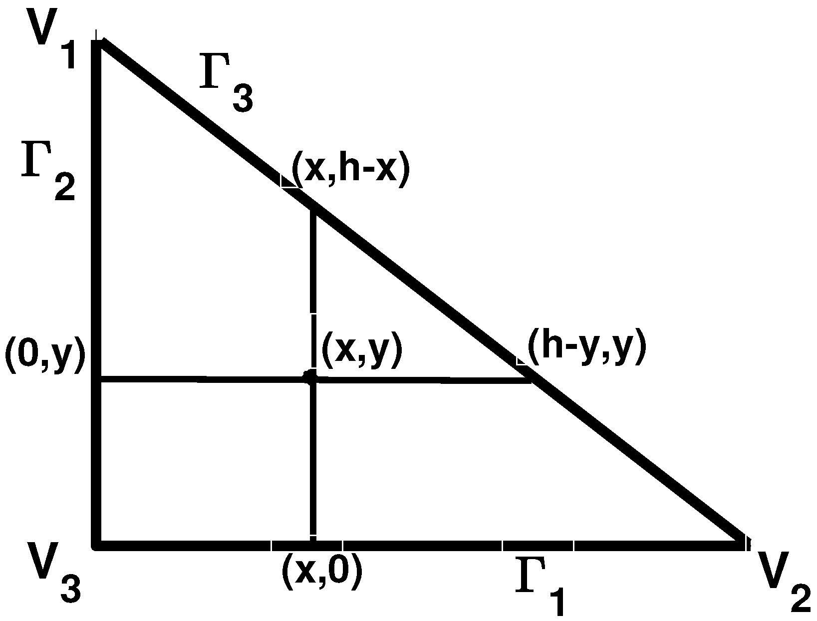
We have considered the standard triangle $T_h$ (see Figure 1), with vertices $V_1=(0,h),$$V_2=(h,0)$ and $V_3=(0,0)$ and sides ${\mathrm{\Gamma }}_1$, ${\mathrm{\Gamma }}_2$, ${\mathrm{\Gamma }}_3$.

2. Cheney–Sharma Operator of the Second Kind

Let $m\in \mathbb{N}$ and $\beta$ be a nonnegative parameter. The Cheney–Sharma operator of the second kind $Q_m:C[0,1]\to C[0,1]$, introduced in [23], is given by

$$\left(Q_{m}f\right)\left(x\right)=\sum _{i=0}^m{q}_{m,i}\left(x\right)f\left(\frac{i}{m}\right),$$

(1)

with

$$q_{m,i}\left(x\right)=\left(\genfrac{}{}{0pt}{}{m}{i}\right)\frac{x{(x+i\beta )}^{i-1}(1-x){[1-x+(m-i)\beta ]}^{m-i-1}}{{(1+m\beta )}^{m-1}}.$$

The following results are useful in the sequel.

Remark 1.

(1) Notice that for $\beta =0$, the operator $Q_m$ becomes the Bernstein operator.

(2) In [25], it has been proved that the Cheney–Sharma operator $Q_m$ interpolates a given function at the endpoints of the interval.

(3) In [23,25], it has been proved that the Cheney–Sharma operator $Q_m$ reproduces the constant and the linear functions, so its degree of exactness is 1 (denoted $dex\left(Q_m\right)=1)$.

(4) In [23], the following result is given:

$$\begin{array}{cc}\hfill \left(Q_m{e}_2\right)\left(x\right)=& x{(1+m\beta )}^{1-m}[S(2,m-2,x+2\beta ,1-x)\hfill \\ \hfill & -(m-2)\beta S(2,m-3,x+2\beta ,1-x+\beta )],\hfill \end{array}$$

(2)

where $e_i\left(x\right)=x^i,$$i\in \mathbb{N},$ and

$$S(j,m,x,y)=\sum _{k=0}^m\left(\genfrac{}{}{0pt}{}{m}{k}\right){(x+k\beta )}^{k+j-1}{[y+(m-k)\beta ]}^{m-k},$$

(3)

$j=0,\dots ,m$, $m\in \mathbb{N}$, $x,y\in [0,1]$, $\beta >0$.

Considering the partitions ${\mathrm{\Delta }}_m^x=\left\{\left.i\frac{h-y}{m}\right|i=0,\dots ,m\right\}$ and ${\mathrm{\Delta }}_n^y=\left\{\left.j\frac{h-x}{n}\right|j=0,\dots ,n\right\}$ of the intervals $[0,h-y]$ and $[0,h-x],$ the real-valued function F defined on $T_h$ (Figure 1), for $m,n\in \mathbb{N},$$\beta ,b\in {\mathbb{R}}_{+},$ we introduce the following extensions to the triangle $T_h$ of the Cheney–Sharma operator given in (1):

$$\begin{array}{cc}\hfill \left(Q_m^{x}F\right)(x,y)& =\sum _{i=0}^m{q}_{m,i}(x,y)F\left(i\frac{h-y}{m},y\right),\hfill \\ \hfill \left(Q_n^{y}F\right)(x,y)& =\sum _{j=0}^n{q}_{n,j}(x,y)F\left(x,j\frac{h-x}{n}\right),\hfill \end{array}$$

(4)

with

$$\begin{array}{cc}\hfill q_{m,i}\left(x,y\right)& =\left(\genfrac{}{}{0pt}{}{m}{i}\right)\frac{\frac{x}{h-y}{(\frac{x}{h-y}+i\beta )}^{i-1}(1-\frac{x}{h-y}){[1-\frac{x}{h-y}+(m-i)\beta ]}^{m-i-1}}{{(1+m\beta )}^{m-1}},\hfill \\ \hfill q_{n,j}\left(x,y\right)& =\left(\genfrac{}{}{0pt}{}{n}{j}\right)\frac{\frac{y}{h-x}{(\frac{y}{h-x}+jb)}^{j-1}(1-\frac{y}{h-x}){[1-\frac{y}{h-x}+(n-j)b]}^{n-j-1}}{{(1+nb)}^{n-1}}.\hfill \end{array}$$

Remark 2.

As the Cheney–Sharma operator of the second kind interpolates a given function at the endpoints of the interval, we may use the operators $Q_m^x$ and $Q_n^y$ as interpolation operators.

Theorem 1.

If F is a real-valued function defined on $T_h$, then

(i)

$Q_m^{x}F=F$ on ${\mathrm{\Gamma }}_1\cup {\mathrm{\Gamma }}_3,$

(ii)

$Q_n^{y}F=F$ on ${\mathrm{\Gamma }}_2\cup {\mathrm{\Gamma }}_3.$

Proof. 

(i) We may write

$$\begin{array}{cc}\hfill \left(Q_m^{x}F\right)(x,y)=& \frac{1}{{(1+m\beta )}^{m-1}}\left\{(1-\frac{x}{h-y}){[1-\frac{x}{h-y}+m\beta ]}^{m-1}F\left(0,y\right)\right.\hfill \\ \hfill & +\frac{x}{h-y}(1-\frac{x}{h-y})\sum _{i=1}^{m-1}\left(\genfrac{}{}{0pt}{}{m}{i}\right){(\frac{x}{h-y}+i\beta )}^{i-1}\hfill \\ \hfill & ·{[1-\frac{x}{h-y}+(m-i)\beta ]}^{m-i-1}F\left(i\frac{h-y}{m},y\right)\hfill \\ \hfill & \left.+\frac{x}{h-y}{(\frac{x}{h-y}+m\beta )}^{m-1}F\left(h-y,y\right)\right\}.\hfill \end{array}$$

(5)

Considering (5), it follows that

$$\begin{array}{cc}\hfill & \left(Q_m^{x}F\right)(0,y)=F(0,y),\hfill \\ \hfill & \left(Q_m^{x}F\right)(h-y,y)=F(h-y,y).\hfill \end{array}$$

(ii) Similarly, writing

$$\begin{array}{cc}\hfill \left(Q_n^{y}F\right)(x,y)=& \frac{1}{{(1+nb)}^{n-1}}\left\{(1-\frac{y}{h-x}){[1-\frac{y}{h-x}+nb]}^{n-1}F\left(x,0\right)\right.\hfill \\ \hfill & +\frac{y}{h-x}(1-\frac{y}{h-x})\sum _{j=1}^{n-1}\left(\genfrac{}{}{0pt}{}{n}{j}\right){(\frac{y}{h-x}+jb)}^{j-1}\hfill \\ \hfill & ·{[1-\frac{y}{h-x}+(n-j)b]}^{n-j-1}F\left(x,j\frac{h-x}{n}\right)\hfill \\ \hfill & \left.+\frac{y}{h-x}{(\frac{y}{h-x}+nb)}^{n-1}F\left(x,h-x\right)\right\},\hfill \end{array}$$

we find that

$$\begin{array}{cc}\hfill & \left(Q_n^{y}F\right)(x,0)=F(x,0),\hfill \\ \hfill & \left(Q_n^{y}F\right)(x,h-x)=F(x,h-x).\hfill \end{array}$$

□

Theorem 2.

The operators $Q_m^x$ and $Q_n^y$ have the following orders of accuracy:

(i)

$\left(Q_m^x{e}_{kj}\right)\left(x,y\right)=x^k{y}^j,k=0,1$; $j\in \mathbb{N}$;

(ii)

$\left(Q_n^y{e}_{kj}\right)\left(x,y\right)=x^k{y}^j$, $k\in \mathbb{N}$; $j=0,1$, where $e_{kj}\left(x,y\right)=x^k{y}^j$, $k,j\in \mathbb{N}$.

Proof. 

(i) We have

$$\left(Q_m^x{e}_{kj}\right)(x,y)=y^j\sum _{i=0}^m{q}_{m,i}(x,y){\left(i\frac{h-y}{m}\right)}^k,$$

and by Remark 1, the result follows.

Similarly, (ii) follows. □

We consider the approximation formula

$$F=Q_m^{x}F+R_m^{x}F,$$

where $R_m^{x}F$ denotes the approximation error.

Theorem 3.

If $F(·,y)\in C[0,h-y]$, the following holds:

$$\left|\left(R_m^{x}F\right)(x,y)\right|\le (1+\frac{1}{\delta }\sqrt{A_m-x^2})\omega (F(·,y);\delta ),\forall \delta >0,$$

(6)

where $\omega \left(F\right(·,y);\delta )$ is the modulus of continuity and $A_m=x{(1+m\beta )}^{1-m}\left[S\right(2,m-2,x+2\beta$, $1-x)-(m-2\left)\beta S\right(2,m-3,x+2\beta ,1-x+\beta \left)\right],$ with S given in (3).

Proof. 

By Theorem 2, it follows that $dex\left(Q_m^x\right)=1$; thus, we may apply the following property of linear operators (see, for example, [35]):

$$|\left(Q_m^{x}F\right)(x,y)-F(x,y)|\le [1+{\delta }^{-1}\sqrt{\left(Q_m^x{e}_{20}\right)(x,y)-x^2}]\omega (F(·,y);\delta ),\forall \delta >0;$$

thus, taking into account (2), we obtain (6). □

Theorem 4.

If $F(·,y)\in C^2[0,h-y]$, then

$$\begin{array}{cc}\hfill \left(R_m^{x}F\right)(x,y)=& \frac{1}{2}{F}^{(2,0)}(\xi ,y)\{x^2-x{(1+m\beta )}^{1-m}[S(2,m-2,x+2\beta ,1-x)\hfill \\ \hfill & -(m-2)\beta S(2,m-3,x+2\beta ,1-x+\beta )\left]\right\},\hfill \end{array}$$

(7)

for $\xi \in [0,h-y]$ and $\beta >0.$

Proof. 

Taking into account the fact that $dex\left(Q_m^x\right)=1,$ by Theorem 2 and applying Peano’s theorem (see, e.g., [36]), it follows that

$$\left(R_m^{x}F\right)(x,y)={\int }_0^{h-y}{K}_{20}(x,y;s)F^{(2,0)}(s,y)ds,$$

where

$$K_{20}(x,y;s)={(x-s)}_{+}-\sum _{i=0}^m{q}_{m,i}(x,y){\left(i\frac{h-y}{m}-s\right)}_{+}.$$

For a given $\nu \in \{1,\dots ,m\}$, one denotes by $K_{20}^{\nu }(x,y;·)$ the restriction of the kernel $K_{20}(x,y;·)$ to the interval $\left. [(\nu -1)\frac{h-y}{m},\nu \frac{h-y}{m}\right],$ i.e.,

$$K_{20}^{\nu }(x,y;\nu )={(x-s)}_{+}-\sum _{i=\nu }^m{q}_{m,i}(x,y)\left(i\frac{h-y}{m}-s\right),$$

whence,

$$K_{20}^{\nu }(x,y;s)=\left\{\begin{array}{cc}x-s-{\displaystyle \sum _{i=\nu }^m}{q}_{m,i}(x,y)\left(i\frac{h-y}{m}-s\right),\hfill & s<x\hfill \\ -{\displaystyle \sum _{i=\nu }^m}{q}_{m,i}(x,y)\left(i\frac{h-y}{m}-s\right),\hfill & s\ge x.\hfill \end{array}\right.$$

It follows that $K_{20}^{\nu }(x,y;s)\le 0,$ for $s\ge x.$

For $s<x$, we have

$$K_{20}^{\nu }(x,y;s)=x-s-{\sum }_{i=0}^m{q}_{m,i}(x,y)\left(i\frac{h-y}{m}-s\right)+{\sum }_{i=0}^{\nu -1}{q}_{m,i}(x,y)\left(i\frac{h-y}{m}-s\right).$$

Applying Theorem 2, we get

$$\sum _{i=0}^m{q}_{m,i}(x,y)\left(i\frac{h-y}{m}-s\right)=\left(Q_m^x{e}_{10}\right)(x,y)-s\left(Q_m^x{e}_{00}\right)(x,y)=x-s;$$

it then follows that

$$K_{20}^{\nu }(x,y;s)=\sum _{i=0}^{\nu -1}{q}_{m,i}(x,y)\left(i\frac{h-y}{m}-s\right)\le 0.$$

Thus, $K_{20}^{\nu }(x,y;·)\le 0,$ for any $\nu \in \{1,\dots ,m\},$ i.e., $K_{20}(x,y;s)\le 0,$ for $s\in [0,h-y].$

By the Mean Value Theorem, one obtains

$$\left(R_m^{x}F\right)(x,y)=F^{(2,0)}(\xi ,y){\int }_0^{h-y}{K}_{20}(x,y;s)ds,\mathrm{for}0\le \xi \le h-y,$$

with

$${\int }_0^{h-y}{K}_{20}(x,y;s)ds=\frac{1}{2}[x^2-\left(Q_m^x{e}_{20}\right)(x,y)],$$

and using (2) we get (7). □

Remark 3.

Analogous results with the ones in Theorems 3 and 4 can be obtained for the remainder $R_n^{y}F$ of the formula $F=Q_n^{y}F+R_n^{y}F.$

2.1. Product Operators

Let $P_{mn}^1=Q_m^x{Q}_n^y,$ respectively, $P_{nm}^2=Q_n^y{Q}_m^x$ be the products of the operators $Q_m^x$ and $Q_n^y,$ given by

$$\left(P_{mn}^{1}F\right)\left(x,y\right)=\sum _{i=0}^m\sum _{j=0}^n{q}_{m,i}\left(x,y\right)q_{n,j}\left(i\frac{h-y}{m},y\right)F\left(i\frac{h-y}{m},j\frac{(m-i)h+iy}{mn}\right),$$

respectively,

$$\left(P_{nm}^{2}F\right)\left(x,y\right)=\sum _{i=0}^m\sum _{j=0}^n{q}_{m,i}\left(x,j\frac{h-x}{n}\right)q_{n,j}\left(x,y\right)F\left(i\frac{(n-j)h+jx}{mn},j\frac{h-x}{n}\right).$$

Theorem 5.

If F is a real-valued function defined on $T_h$, then

(i) 

$\left(P_{mn}^{1}F\right)\left(V_i\right)=F\left(V_i\right),i=1,2,3;$

$\left(P_{mn}^{1}F\right)\left({\mathrm{\Gamma }}_3\right)=F\left({\mathrm{\Gamma }}_3\right),$

(ii) 

$\left(P_{nm}^{2}F\right)\left(V_i\right)=F\left(V_i\right),i=1,2,3;$

$\left(P_{nm}^{2}F\right)\left({\mathrm{\Gamma }}_3\right)=F\left({\mathrm{\Gamma }}_3\right),$

Proof. 

By a straightforward computation, we obtain the following properties:

$$\begin{array}{cc}\hfill & \left(P_{mn}^{1}F\right)(x,0)=\left(Q_m^{x}F\right)(x,0),\hfill \\ \hfill & \left(P_{mn}^{1}F\right)(0,y)=\left(Q_n^{y}F\right)(0,y),\hfill \\ \hfill & \left(P_{mn}^{1}F\right)(x,h-x)=F(x,h-x),x,y\in [0,h]\hfill \end{array}$$

and

$$\begin{array}{cc}\hfill & \left(P_{nm}^{2}F\right)(x,0)=\left(Q_m^{x}F\right)(x,0),\hfill \\ \hfill & \left(P_{nm}^{2}F\right)(0,y)=\left(Q_n^{y}F\right)(0,y),\hfill \\ \hfill & \left(P_{nm}^{2}F\right)(h-y,y)=F(h-y,y),x,y\in [0,h],\hfill \end{array}$$

and, taking into account Theorem 1, these imply (i) and (ii). □

We consider the following approximation formula:

$$F=P_{mn}^{1}F+R_{mn}^{{}^{P^1}}F,$$

where $R_{mn}^{{}^{P^1}}$ is the corresponding remainder operator.

Theorem 6.

If $F\in C\left(T_h\right)$ then

$$\left|(R_{mn}^{P^1}F)(x,y)\right|\le (A_m+B_n-x^2-y^2+1)\omega (F;\frac{1}{\sqrt{A_m-x^2}},\frac{1}{\sqrt{B_n-y^2}}),\forall (x,y)\in T_h,$$

(8)

where

$$\begin{array}{cc}\hfill A_m=& x{(1+m\beta )}^{1-m}[S(2,m-2,x+2\beta ,1-x)\hfill \\ \hfill & -(m-2)\beta S(2,m-3,x+2\beta ,1-x+\beta )]\hfill \\ \hfill B_n=& y{(1+nb)}^{1-n}[S(2,n-2,y+2b,1-y)-(n-2)bS(2,n-3,y+2b,1-y+\beta )]\hfill \end{array}$$

(9)

and $\omega (F;{\delta }_1,{\delta }_2)$, with ${\delta }_1>0,$ ${\delta }_2>0,$ is the bivariate modulus of continuity.

Proof. 

Using a basic property of the modulus of continuity, we have

$$\begin{array}{cc}\hfill \left|\left(R_{mn}^{P^1}F\right)(x,y)\right|\le & [\frac{1}{{\delta }_1}\sum _{i=0}^m\sum _{j=0}^n{q}_{m,i}(x,y)q_{n,j}\left(\frac{i}{m}(h-y),y\right)\left|x-\frac{i}{m}(h-y)\right|\hfill \\ \hfill & +\frac{1}{{\delta }_2}\sum _{i=0}^m\sum _{j=0}^n{q}_{m,i}(x,y)q_{n,j}\left(\frac{i}{m}(h-y),y\right)\left|y-\frac{j}{n}\frac{(m-i)h+iy}{m}\right|\hfill \\ \hfill & +\sum _{i=0}^m\sum _{j=0}^n{q}_{m,i}(x,y)q_{n,j}\left(\frac{i}{m}(h-y),y\right)]\omega (F;{\delta }_1,{\delta }_2),\forall {\delta }_1,{\delta }_2>0.\hfill \end{array}$$

Since

$$\begin{array}{cc}\hfill & \sum _{i=0}^m\sum _{j=0}^n{p}_{m,i}(x,y)q_{n,j}\left(\frac{i}{m}(h-y),y\right)\left|x-\frac{i}{m}(h-y)\right|\le \sqrt{\left(Q_m^x{e}_{20}\right)(x,y)-x^2},\hfill \\ \hfill & \sum _{i=0}^m\sum _{j=0}^n{p}_{m,i}(x,y)q_{n,j}\left(\frac{i}{m}(h-y),y\right)\left|y-\frac{j}{n}\frac{(m-i)h+iy}{m}\right|\le \sqrt{\left(Q_n^y{e}_{02}\right)(x,y)-y^2},\hfill \\ \hfill & \sum _{i=0}^m\sum _{j=0}^n{p}_{m,i}(x,y)q_{n,j}\left(\frac{i}{m}(h-y),y\right)=1,\hfill \end{array}$$

applying (2), we get

$$\begin{array}{cc}\hfill & \left|\left(R_{mn}^{P^1}F\right)(x,y)\right|\le \{\frac{1}{{\delta }_1}{\left[x{(1+m\beta )}^{1-m}\right]}^{\frac{1}{2}}\hfill \\ \hfill & ·{\left\{[S(2,m-2,x+2\beta ,1-x)-(m-2)\beta S(2,m-3,x+2\beta ,1-x+\beta )]-x^2\right\}}^{\frac{1}{2}}\hfill \\ \hfill & +\frac{1}{{\delta }_2}{\left[y{(1+nb)}^{1-n}\right]}^{\frac{1}{2}}\hfill \\ \hfill & ·{\left\{[S(2,n-2,y+2b,1-y)-(n-2)bS(2,n-3,y+2b,1-y+\beta )]-y^2\right\}}^{\frac{1}{2}}\left.+1\right\}\omega (F;{\delta }_1,{\delta }_2).\hfill \end{array}$$

Denoting

$$\begin{array}{cc}\hfill A_m& =x{(1+m\beta )}^{1-m}[S(2,m-2,x+2\beta ,1-x)-(m-2)\beta S(2,m-3,x+2\beta ,1-x+\beta )]\hfill \\ \hfill B_n& =y{(1+nb)}^{1-n}[S(2,n-2,y+2b,1-y)-(n-2)bS(2,n-3,y+2b,1-y+\beta )]\hfill \end{array}$$

and taking ${\delta }_1=\frac{1}{\sqrt{A_m-x^2}}$ and ${\delta }_2=\frac{1}{\sqrt{B_n-y^2}}$, we get (8). □

2.2. Boolean Sum Operators

The Boolean sums of the operators $Q_m^x$ and $Q_n^y$ are given by

$$\begin{array}{cc}\hfill S_{mn}^1& :=Q_m^x\oplus Q_n^y=Q_m^x+Q_n^y-Q_m^x{Q}_n^y,\hfill \\ \hfill S_{nm}^2& :=Q_n^y\oplus Q_m^x=Q_n^y+Q_m^x-Q_n^y{Q}_m^x.\hfill \end{array}$$

Theorem 7.

If F is a real-valued function defined on $T_h,$ then

$$\begin{array}{cc}\hfill & S_{mn}^{1}F{\left|{}_{\partial T_h}=F\right|}_{\partial T_h},\hfill \\ \hfill & S_{mn}^{2}F{\left|{}_{\partial T_h}=F\right|}_{\partial T_h}.\hfill \end{array}$$

Proof. 

By

$$\begin{array}{cc}\hfill \left(Q_m^x{Q}_n^{y}F\right)\left(x,0\right)=& \left(Q_m^{x}F\right)\left(x,0\right),\hfill \\ \hfill \left(Q_n^y{Q}_m^{x}F\right)\left(0,y\right)=& \left(Q_n^{y}F\right)\left(0,y\right),\hfill \\ \hfill \left(Q_m^{x}F\right)\left(x,h-x\right)=& \left(Q_n^{y}F\right)(x,h-x)\hfill \\ \hfill & =\left(P_{mn}^{1}F\right)(x,h-x)=\left(P_{nm}^{2}F\right)(x,h-x)=F(x,h-x),\hfill \end{array}$$

and, taking into account Theorem 1, the conclusion follows. □

We consider the following approximation formula:

$$F=S_{mn}^{1}F+R_{mn}^{{}^{S^1}}F,$$

where $R_{mn}^{{}^{S^1}}$ is the corresponding remainder operator.

Theorem 8.

If $F\in C\left(T_h\right)$, then

$$\begin{array}{cc}\hfill & \left|(R_{mn}^{{}^{S^1}}F)(x,y)\right|\le \hfill \\ \hfill & \le (1+A_m-x^2)\omega (F(·,y);\frac{1}{\sqrt{A_m-x^2}})+(1+B_n-y^2)\omega (F(x,·);\frac{1}{\sqrt{B_n-y^2}})\hfill \\ \hfill & +(A_m+B_n-x^2-y^2+1)\omega (F;\frac{1}{\sqrt{A_m-x^2}},\frac{1}{\sqrt{B_n-y^2}}),\hfill \end{array}$$

(10)

with $A_m$ and $B_n$ given in (9).

Proof. 

The identity

$$F-S_{mn}^{1}F=(F-Q_m^{x}F)+(F-Q_n^{y}F)-(F-P_{mn}^{1}F)$$

implies that

$$\left|\left(R_{mn}^{{}^{S^1}}F\right)(x,y)\right|\le \left|\left(R_m^{x}F\right)(x,y)\right|+\left|\left(R_n^{y}F\right)(x,y)\right|+\left|\left(R_{mn}^{P^1}F\right)(x,y)\right|,$$

and, applying Theorems 3 and 6, we get (10). □

3. Cheney–Sharma Operator of the First Kind

Let $m\in N$ and $\beta$ be a nonnegative parameter. In [23], based on the following Jensen’s identity,

$${(x+y+m\beta )}^m=\sum _{k=0}^m\left(\genfrac{}{}{0pt}{}{m}{k}\right)x{(x+k\beta )}^{k-1}{[y+(m-k)\beta ]}^{m-k},(\forall )(x,y)\in {\mathbb{R}}^2,$$

the Cheney–Sharma operators of the first kind $G_m:C[0,1]\to C[0,1]$ were introduced, given by

$$\left(G_{m}f\right)\left(x\right)=\sum _{i=0}^m{q}_{m,i}\left(x\right)f(\frac{k}{m}),$$

with

$$q_{m,i}\left(x\right)=\left(\genfrac{}{}{0pt}{}{m}{i}\right)\frac{x{(x+i\beta )}^{i-1}{[1-x+(m-i)\beta ]}^{m-i}}{{(1+m\beta )}^m}.$$

For F, a real-valued function defined on $T_h,$$m,n\in \mathbb{N},$ $\beta ,b\in {\mathbb{R}}_{+},$ and the uniform partitions ${\mathrm{\Delta }}_m^x$ and ${\mathrm{\Delta }}_n^y$ of the intervals $[0,h-y]$ and $[0,h-x],$ we consider here the new extensions of the Cheney–Sharma operator of the first kind,

$$\begin{array}{cc}\hfill \left(G_m^{x}F\right)(x,y)& =\sum _{i=0}^m{r}_{m,i}(x,y)F\left(i\frac{h-y}{m},y\right),\hfill \\ \hfill \left(G_n^{y}F\right)(x,y)& =\sum _{j=0}^n{r}_{n,j}(x,y)F\left(x,j\frac{h-x}{n}\right),\hfill \end{array}$$

(11)

with

$$\begin{array}{cc}\hfill r_{m,i}\left(x,y\right)& =\left(\genfrac{}{}{0pt}{}{m}{i}\right)\frac{\frac{x}{h-y}{(\frac{x}{h-y}+i\beta )}^{i-1}{[1-\frac{x}{h-y}+(m-i)\beta ]}^{m-i}}{{(1+m\beta )}^m},\hfill \\ \hfill r_{n,j}\left(x,y\right)& =\left(\genfrac{}{}{0pt}{}{n}{j}\right)\frac{\frac{y}{h-x}{(\frac{y}{h-x}+jb)}^{j-1}{[1-\frac{y}{h-x}+(n-j)b]}^{n-j}}{{(1+nb)}^n}.\hfill \end{array}$$

We denote by $P_{mn}^G=G_m^x{G}_n^y$ the product and by $S_{mn}^G:=G_m^x\oplus G_n^y=G_m^x+G_n^y-G_m^x{G}_n^y$, respectively, the Boolean sum of the operators $G_m^x$ and $G_n^y$.

Remark 4.

The new extensions of the Cheney–Sharma operator of the first kind, $G_m^x$ and $G_n^y,$ and their product and Boolean sum, $P_{mn}^G$ and $S_{mn}^G$, introduced here, have similar properties as the ones of the Cheney–Sharma operator of the second kind from the previous section.

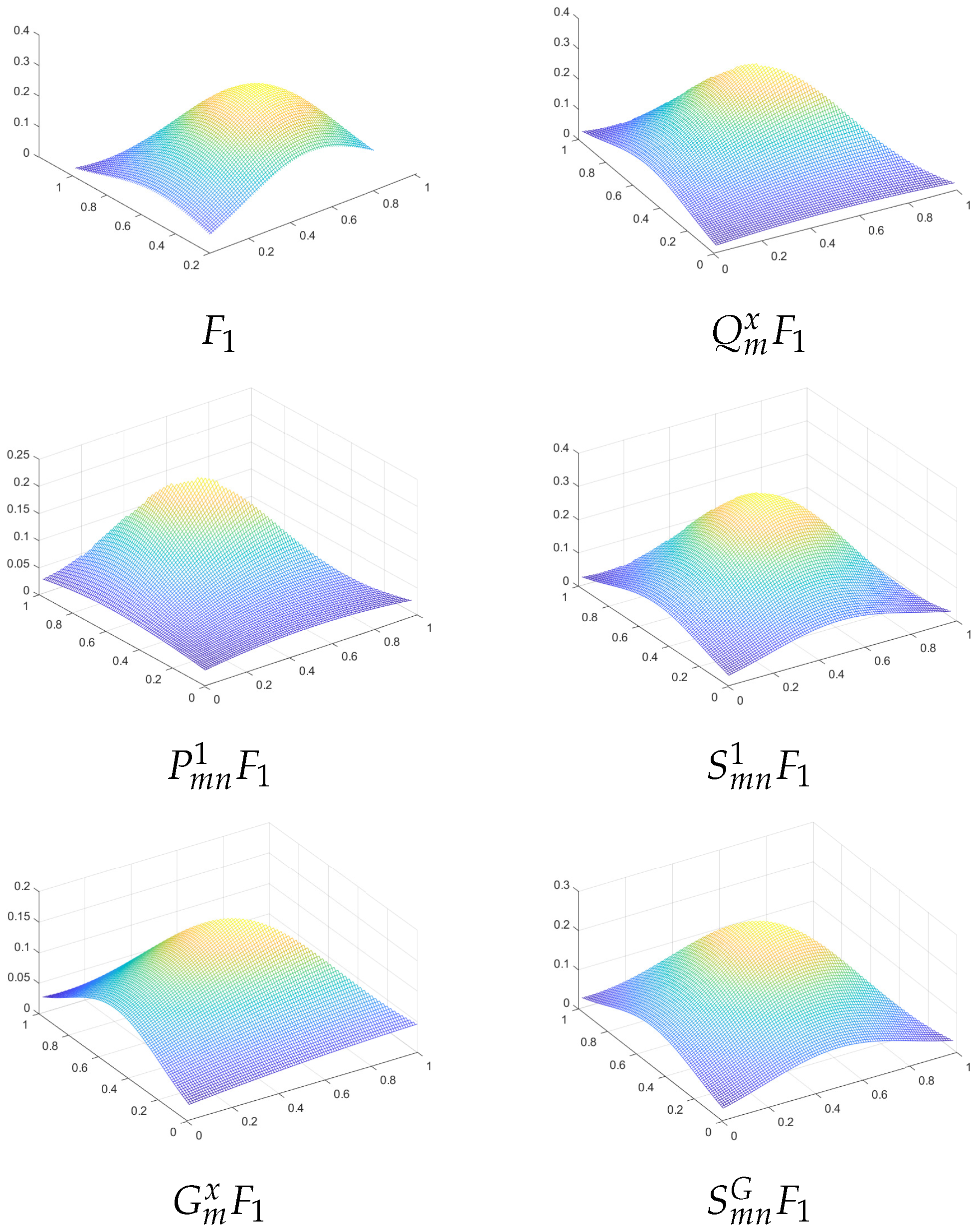
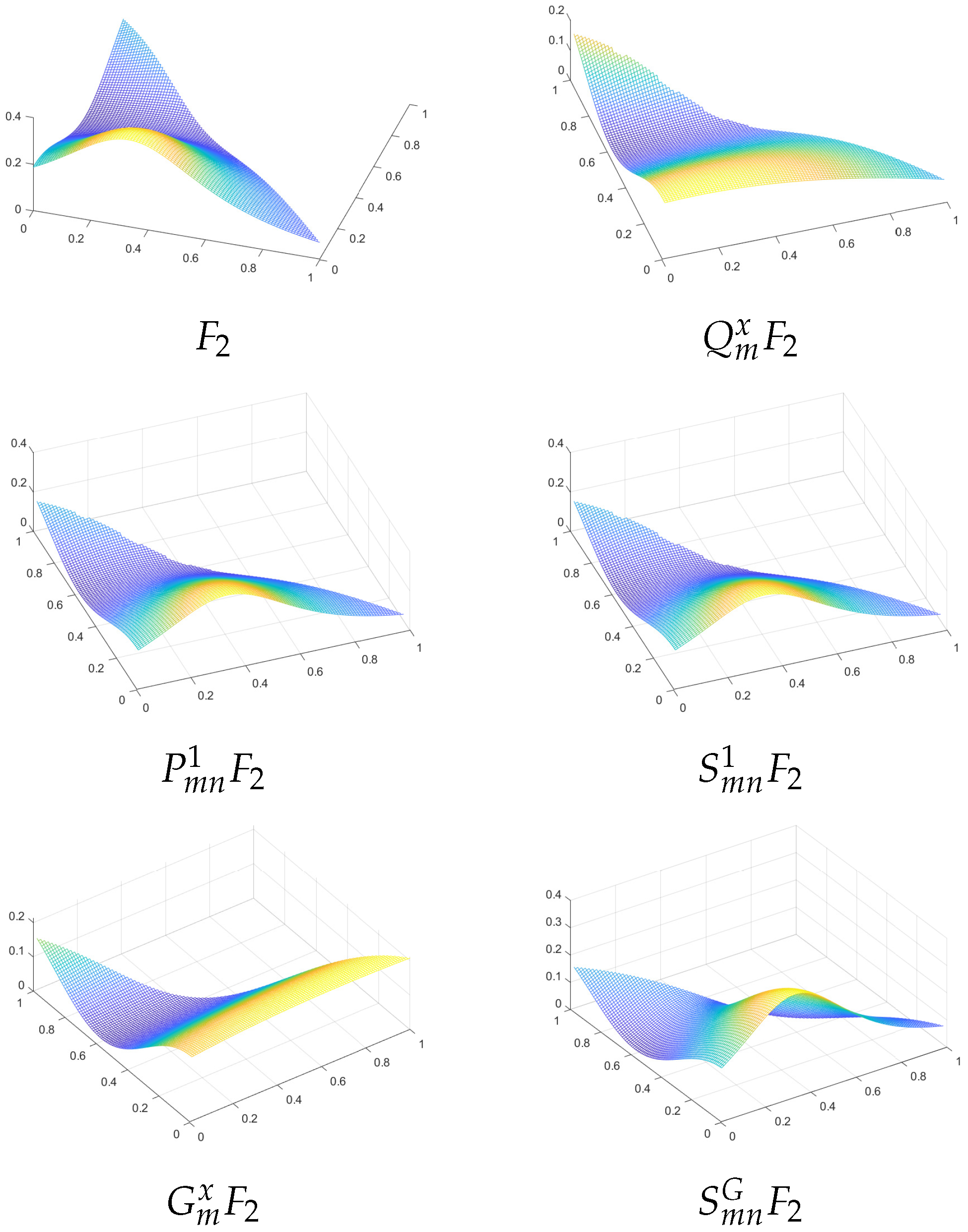
4. Numerical Examples

In this section, we consider two test functions for which we plot the graphs of the approximants using the methods presented here, and also we study the maximum approximation errors for the corresponding approximants.

Example 1.

Consider the following test functions, generally used in the literature (see, e.g., [37]):

$$\begin{array}{c}\mathit{Gentle}\mathit{:}{F}_1(x,y)=\frac{1}{3}exp[-\frac{81}{16}({(x-0.5)}^2+{(y-0.5)}^2)],\hfill \\ \mathit{Saddle}\mathit{:}{F}_2(x,y)={\displaystyle \frac{1.25+cos5.4y}{6+6{(3x-1)}^2}}.\hfill \end{array}$$

(12)

Considering $h=1, m=5,$ $n=6$, $\beta =1$, in

Table 1. Maximum approximation errors.

Max Error	${\mathit{F}}_1$	${\mathit{F}}_2$
$Q_m^x{F}_i$	$0.0862$	$0.1922$
$Q_n^y{F}_i$	$0.1264$	$0.1529$
$P_{mn}^1{F}_i$	$0.1680$	$0.1926$
$S_{mn}^1{F}_i$	$0.0152$	$0.0235$
$G_m^x{F}_i$	$0.1523$	$0.1695$
$G_n^y{F}_i$	$0.1560$	$0.2364$
$P_{mn}^G{F}_i$	$0.2444$	$0.1697$
$S_{mn}^G{F}_i$	$0.0676$	$0.0750$

, one can see the maximum errors for approximating $F_i$ by $Q_m^x{F}_i,$ $Q_n^y{F}_i,$ $P_{mn}^1{F}_i,$ $S_{mn}^1{F}_i$, $G_m^x{F}_i,G_n^y{F}_i,$ $P_{mn}^G{F}_i,$ $S_{mn}^G{F}_i$, $i=1,2;$ in Figure 2 and Figure 3, we have plotted the graphs of $F_i,$ $Q_m^x{F}_i,$ $Q_n^y{F}_i,$ $P_{mn}^1{F}_i,$ $S_{mn}^1{F}_i$, $G_m^x{F}_i,S_{mn}^G{F}_i,$ $i=1,2$ on $T_h.$

5. Conclusions

According to Table 1 and Figure 2 and Figure 3, we note the good approximation properties of the two types of Cheney–Sharma operators considered here, especially of the Boolean sum operators, which interpolate on the entire frontier of the domain.

References

- Barnhill, R.E.; Birkhoff, G.; Gordon, W.J. Smooth interpolation in triangles. J. Approx. Theory 1973, 8, 114–128. [Google Scholar] [CrossRef] [Green Version]
- Barnhill, R.E.; Gregory, J.A. Polynomial interpolation to boundary data on triangles. Math. Comp. 1975, 29, 726–735. [Google Scholar] [CrossRef]
- Blaga, P.; Coman, G. Bernstein-type operators on triangle. Rev. Anal. Numer. Theor. Approx. 2009, 37, 9–21. [Google Scholar]
- Böhmer, K.; Coman, G. Blending Interpolation Schemes on Triangle with Error Bounds; Lecture Notes in Mathematics, 571; Springer: Berlin/Heidelberg, Germany; New York, NY, USA, 1977; pp. 14–37. [Google Scholar]
- Cătinaş, T.; Coman, G. Some interpolation operators on a simplex domain. Stud. Univ. Babes-Bolyai Math. 2007, 52, 25–34. [Google Scholar]
- Costabile, F.A.; Dell’Accio, F. Expansions over a simplex of real functions by means of Bernoulli polynomials. Numer. Algorithms 2001, 28, 63–86. [Google Scholar] [CrossRef]
- Costabile, F.A.; Dell’Accio, F. Lidstone approximation on the triangle. Appl. Numer. Math. 2005, 52, 339–361. [Google Scholar] [CrossRef]
- Barnhill, R.E.; Gregory, J.A. Compatible smooth interpolation in triangles. J. Approx. Theory 1975, 15, 214–225. [Google Scholar] [CrossRef] [Green Version]
- Bernardi, C. Optimal finite-element interpolation on curved domains. SIAM J. Numer. Anal. 1989, 26, 1212–1240. [Google Scholar] [CrossRef]
- Blaga, P.; Cătinaş, T.; Coman, G. Bernstein-type operators on tetrahedrons. Stud. Univ. Babes-Bolyai Math. 2009, 54, 3–19. [Google Scholar]
- Blaga, P.; Cătinaş, T.; Coman, G. Bernstein-type operators on a square with one and two curved sides. Stud. Univ. Babes-Bolyai Math. 2010, 55, 51–67. [Google Scholar]
- Blaga, P.; Cătinaş, T.; Coman, G. Bernstein-type operators on triangle with all curved sides. Appl. Math. Comput. 2011, 218, 3072–3082. [Google Scholar] [CrossRef]
- Blaga, P.; Cătinaş, T.; Coman, G. Bernstein-type operators on triangle with one curved side. Mediterr. J. Math. 2012, 9, 843–855. [Google Scholar] [CrossRef]
- Cătinaş, T. Some classes of surfaces generated by Nielson and Marshall type operators on the triangle with one curved side. Stud. Univ. Babes-Bolyai Math. 2016, 61, 305–314. [Google Scholar]
- Cătinaş, T. Extension of some particular interpolation operators to a triangle with one curved side. Appl. Math. Comput. 2017, 315, 286–297. [Google Scholar] [CrossRef]
- Cătinaş, T. Extension of Some Cheney-Sharma Type Operators to a Triangle With One Curved Side. Miskolc Math. Notes 2020, 21, 101–111. [Google Scholar] [CrossRef]
- Cătinaş, T.; Blaga, P.; Coman, G. Surfaces generation by blending interpolation on a triangle with one curved side. Results Math. 2013, 64, 343–355. [Google Scholar] [CrossRef]
- Coman, G.; Cătinaş, T. Interpolation operators on a tetrahedron with three curved sides. Calcolo 2010, 47, 113–128. [Google Scholar] [CrossRef]
- Coman, G.; Cătinaş, T. Interpolation operators on a triangle with one curved side. BIT Numer. Math. 2010, 50, 243–267. [Google Scholar] [CrossRef]
- Marshall, J.A.; Mitchell, A.R. An exact boundary tehnique for improved accuracy in the finite element method. J. Inst. Maths. Applics. 1973, 12, 355–362. [Google Scholar] [CrossRef]
- Mitchell, A.R.; McLeod, R. Curved elements in the finite element method. In Conference on the Numerical Solution of Differential Equations; Springer: Berlin/Heidelberg, Germany, 1974; Volume 363, pp. 89–104. [Google Scholar]
- Chandra, P.; Kumar, V.D.; Naokant, D. Approximation by Durrmeyer variant of Cheney-Sharma Chlodovsky operators. Math. Found. Comput. 2022. [Google Scholar] [CrossRef]
- Cheney, E.W.; Sharma, A. On a generalization of Bernstein polynomials. Riv. Mat. Univ. Parma 1964, 5, 77–84. [Google Scholar]
- Ong, S.H.; Ng, C.M.; Yap, H.K.; Srivastava, H.M. Some Probabilistic Generalizations of the Cheney–Sharma and Bernstein Approximation Operators. Axioms 2022, 11, 537. [Google Scholar] [CrossRef]
- Stancu, D.D.; Cişmaxsxiu, C. On an approximating linear positive operator of Cheney-Sharma. Rev. Anal. Numer. Theor. Approx. 1997, 26, 221–227. [Google Scholar]
- Barnhill, R.E. Blending Function Interpolation: A Survey and Some New Results. In Numerishe Methoden der Approximationstheorie; Collatz, L., Ed.; Birkhauser-Verlag: Basel, Switzerland, 1976; Volume 30, pp. 43–89. [Google Scholar]
- Barnhill, R.E. Representation and approximation of surfaces. In Mathematical Software III; Rice, J.R., Ed.; Academic Press: New York, NY, USA, 1977; pp. 68–119. [Google Scholar]
- Barnhill, R.E.; Gregory, J.A. Sard kernels theorems on triangular domains with applications to finite element error bounds. Numer. Math. 1976, 25, 215–229. [Google Scholar] [CrossRef]
- Gordon, W.J.; Hall, C. Transfinite element methods: Blending-function interpolation over arbitrary curved element domains. Numer. Math. 1973, 21, 109–129. [Google Scholar] [CrossRef]
- Gordon, W.J.; Wixom, J.A. Pseudo-harmonic interpolation on convex domains. SIAM J. Numer. Anal. 1974, 11, 909–933. [Google Scholar] [CrossRef]
- Liu, T. A wavelet multiscale-homotopy method for the parameter identification problem of partial differential equations. Comput. Math. Appl. 2016, 71, 1519–1523. [Google Scholar] [CrossRef]
- Liu, T. A multigrid-homotopy method for nonlinear inverse problems. Comput. Math. Appl. 2020, 79, 1706–1717. [Google Scholar] [CrossRef]
- Marshall, J.A.; Mitchell, A.R. Blending interpolants in the finite element method. Int. J. Numer. Meth. Eng. 1978, 12, 77–83. [Google Scholar] [CrossRef]
- Roomi, V.; Ahmadi, H.R. Continuity and Differentiability of Solutions with Respect to Initial Conditions and Peano Theorem for Uncertain Differential Equations. Math. Interdiscip. 2022. [Google Scholar] [CrossRef]
- Agratini, O. Approximation by Linear Operators; Cluj University Press: Cluj-Napoca, Romania, 2000. [Google Scholar]
- Sard, A. Linear Approximation; American Mathematical Society: Providence, RI, USA, 1963. [Google Scholar]
- Renka, R.J.; Cline, A.K. A triangle-based C1 interpolation method. Rocky Mountain J. Math. 1984, 14, 223–237. [Google Scholar] [CrossRef]
Figure 1.
Triangle .
Figure 2.
Graphs of and its interpolants on .
Figure 3.