
A Review on Some Linear Positive Operators Defined on Triangles

Faculty of Mathematics and Computer Science, Babeş-Bolyai University, St. M. Kogălniceanu No. 1, RO-400084 Cluj-Napoca, Romania
Symmetry 2022, 14(9), 1880; https://doi.org/10.3390/sym14091880
Submission received: 9 August 2022
/
Revised: 24 August 2022
/
Accepted: 2 September 2022
/
Published: 8 September 2022
(This article belongs to the Special Issue Numerical Analysis, Approximation Theory, Differential Equations)
Abstract
:We consider results regarding Bernstein and Cheney–Sharma-type operators that interpolate functions defined on triangles with straight and curved sides and we introduce a new Cheney–Sharma-type operator for the triangle with one curved side, highlighting the symmetry between the methods. We present some properties of the operators, their products and Boolean sums and some results regarding the remainders of the corresponding approximation formulas, using modulus of continuity and Peano’s theorem. Additionally, we consider some numerical examples to show the approximation properties of the given operators.
Keywords:
Bernstein operator; Cheney–Sharma operator; product and Boolean sum operators; modulus of continuity; degree of exactness; error evaluationMSC:
41A35; 41A36; 41A25; 41A801. Introduction
Certain interpolation operators have been constructed for functions defined on triangles with straight sides (see, e.g., [1,2,3,4,5,6,7,8,9,10]) and for functions defined on domains with curved sides (see, e.g., [11,12,13,14,15,16,17,18,19,20,21,22,23,24]).
Different types of interpolation operators (Lagrange, Hermite, Birkhoff, Bernstein, Cheney–Sharma, Nielson, generalized Hermite) that match all the boundary information on curved domains (triangles, squares) have been constructed and studied by us (see, e.g., [13,14,15,17,18,21,22]). In these works we have studied the properties of the operators, their products and Boolean sums and the remainders of the corresponding approximation formulas, using modulus of continuity and Peano’s theorem.
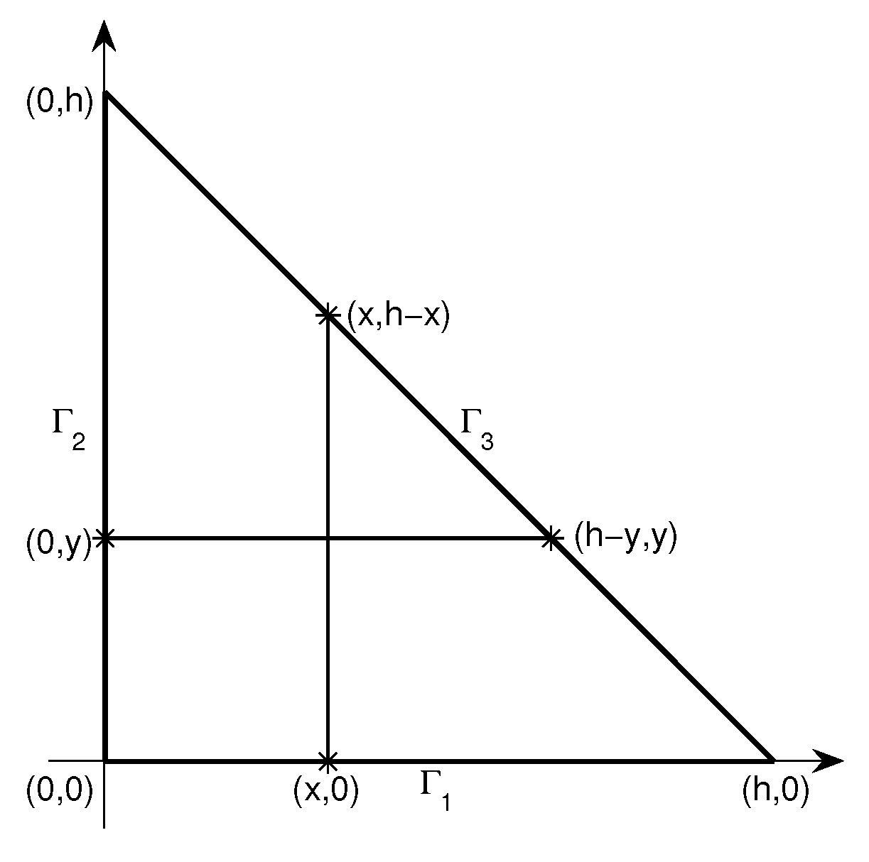
Here we consider two standards triangles. First we consider the standard triangle with all straight sides (see Figure 1), for which if we consider the parallel lines to the coordinate axes through the point , they intersect the sides , , of the triangle at the points and respectively and .
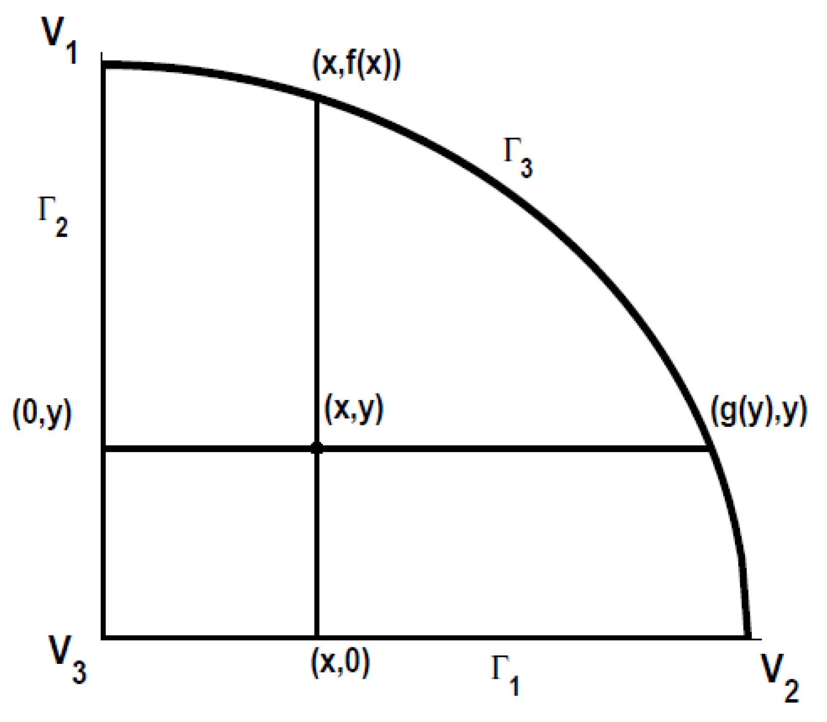
We also consider the standard triangle with one curved side with vertices and with two straight sides along the coordinate axes, and with the third side (opposite to the vertex ) defined by the one-to-one functions f and where g is the inverse of the function i.e., and , with for . Additionally, we have and for The functions f and g are defined as in [2]. Let F be a real-valued function defined on and respectively, be the points at which the parallel lines to the coordinate axes, passing through the point intersect the sides (See Figure 2).
The aim of this paper is to survey results regarding Bernstein- and Cheney–Sharma-type operators that interpolate functions defined on triangles with straight sides and with one curved side, obtained in [3,15,18], and to introduce a new Cheney–Sharma-type operator defined on There is a symmetrical connection between the methods proposed for the triangle with straight sides and the ones for the triangle with curved sides.
Using the interpolation properties of the operators, blending function interpolants can be constructed that exactly match the function on some sides of the given region. There are many important applications of these blending functions in computer-aided geometric design (see, e.g., [1,25,26,27,28]), in finite element method for differential equations (see, e.g., [23,24,25,29,30,31,32]), for construction of surfaces that satisfy some given conditions (see, e.g., [16,20]), in combination with the triangular Shepard method (see, e.g., [33,34]) or in numerical integration formulas (see, e.g., [35]).
The paper is structured in three main sections: Bernstein-type operators, Cheney–Sharma operators of the second kind and Cheney–Sharma operators of the first kind. The first section has two subsections regarding Bernstein-type operators defined on triangle with straight sides and on triangle with one curved side, respectively. The second section has also two subsections regarding the same two types of domains. The last sections contains some new results regarding Cheney–Sharma operators of the first kind defined on triangle with one curved side.
2. Bernstein Type Operator
Since the Bernstein-type operators interpolate a given function at the endpoints of the interval, these operators can also be used as interpolation operators both on triangles with straight sides and with curved sides.
2.1. Bernstein Operator on Triangle with All Straight Sides
Let f be a real-valued function defined on the standard triangle with all straight sides (see Figure 1).
Let and be uniform partitions of the intervals and .
Proof.
The property (ii) follows directly. □
Remark 1.
In the same way there are proved similar results for the operator
Product and Boolean Sum Operators
Let and be given by
Theorem 2
([3]). The operators and satisfy the following relations:
- (i)
- (ii)
- (iii)
The proofs follow by a straightforward computation.
Remark 2.
The product operator interpolates the function f at the vertex and on the hypothenuse of the triangle .
Let consider the Boolean sums of the Bernstein-type operators and , given by
Remark 3.
The Boolean sum is a transfinite (blending) operator.
Theorem 3
Proof.
We have
The result follows by the interpolation properties of , and Theorem 2. □
2.2. Bernstein Operator on Triangle with One Curved Side
Let F be a real-valued function defined on the standard triangle with a curved side (see Figure 2). One considers the Bernstein-type operators and defined by [15]
with
and
with
where
are uniform partitions of the intervals and with and for
Theorem 4
([15]). With the above notations, if F is a real-valued function defined on then:
- (i)
- on
- (ii)
- onand
- (iii)
- (iv)
Proof.
The proof of (i) and (ii) is based on the relations:
and
The properties (iii) and (iv) are obtained directly. □
Theorem 5
([15]). If and then
where is the modulus of continuity of the function F with regard to the variable
Moreover, if then
Proof.
From the property it follows that
Using the inequality
one obtains
Since,
it follows that
hence
For one obtains (1). □
Proof.
The proof is based on Peano’s theorem, taking into account that . □
Product and Boolean Sum Operators
Let and be the products of the operators and
We have [15]
Theorem 7
([15]). If F is a real-valued function defined on then:
- (i)
- onand
- (ii)
- on
Proof.
It results from the properties
and
which can be verified by a straightforward computation. □
Let us consider the approximation formula
where is the corresponding remainder operator.
Theorem 8
Proof.
We have
Since,
it follows that
But
whence,
and
□
We consider the Boolean sums of the operators and i.e.,
Theorem 9
Proof.
The proof follows by a direct verification. □
For the remainder of the Boolean sum approximation formula,
we have the following result.
Theorem 10
Proof.
The identity
implies that
and the conclusion follows. □
3. Cheney–Sharma Operator of the Second Kind
Let and be a nonnegative parameter. In [36], based on the following Jensen’s identity,
it was introduced the Cheney–Sharma operator of second kind , given by
We recall some results regarding these Cheney–Sharma-type operators.
Remark 4.
(1) Notice that for , the operator becomes the Bernstein operator.
(2) In [37] it is proved that the Cheney–Sharma operator interpolates a given function at the endpoints of the interval.
Remark 5.
We may use the Cheney–Sharma operators of second kind and as interpolation operators, because they interpolate a given function at the endpoints of the interval.
3.1. Cheney–Sharma Operator on Triangle with All Straight Sides
Let f be a real-valued function defined on the standard triangle with all straight sides (see Figure 1).
Let and be uniform partitions of the intervals and for .
In [19] we study the Cheney–Sharma operator of the second kind for the functions defined on . We study their interpolation properties, the corresponding product and Boolean sum operators, and the remainders of the interpolation formulas. The operators are given by
with
where
3.2. Cheney–Sharma Operator on Triangle with One Curved Side
Let F be a real-valued function defined on standard triangle with a curved side (see Figure 2). For we have considered the following extensions of the Cheney–Sharma operator of the second kind to the case of functions defined on , see [18]:
with
where
are uniform partitions of the intervals and respectively.
Theorem 11
([18]). If F is a real-valued function defined on then
- (i)
- on
- (ii)
- on
Proof.
(i) We may write
Considering (8), it follows (i).
(ii) Similarly, writing
we get (ii). □
Theorem 12
([18]). The operators and have the following properties:
- (i)
- (ii)
- where
Proof.
The proof is based on the Remark 4. □
We consider the approximation formula
where denotes the approximation error.
Proof.
Theorem 14
Proof.
Taking into account that by Theorem 12, and applying the Peano’s theorem (see, e.g., [39]), it follows
where
For a given one denotes by the restriction of the kernel to the interval i.e.,
whence,
It follows that for
For we have
Applying Theorem 12, we obtain
whence it follows that
So, for any i.e., for
Remark 6.
Analogous results with the ones in Theorems 13 and 14 can be obtained for the remainder of the formula
Product and Boolean Sum Operators
Let and be the products of the operators and
We have
and
Theorem 15
([18]). If F is a real-valued function defined on then
- (i)
- (ii)
Proof.
By a straightforward computation, we obtain the following properties
and
and, taking into account Theorem 11, they imply (i) and (ii). □
We consider the following approximation formula
where is the corresponding remainder operator.
Theorem 16
and , with is the bivariate modulus of continuity.
Proof.
Using a basic property of the modulus of continuity we have
Denoting
and, taking and , we get (11). □
We consider the Boolean sums of the operators and ,
Theorem 17
Proof.
We have
and, taking into account Theorem 11, the conclusion follows. □
We consider the following approximation formula
where is the corresponding remainder operator.
Proof.
4. Cheney–Sharma Operator of the First Kind
Let and be a non-negative parameter. In [36], based on the following Jensen’s identity
it was introduced the Cheney–Sharma operators of the first kind , given by
with
For F a real-valued function defined on we consider here the new extensions of the Cheney–Sharma operator of the first kind,
with
where
are uniform partitions of the intervals and
Remark 7.
The new extensions of the Cheney–Sharma operator of the first kind, introduced here, have similar properties as the ones of the Cheney–Sharma operator of second kind from Section 3.
5. Numerical Examples
In this section, we consider two test functions for which we plot the graphs of the approximants using the methods presented here, and also we study the maximum approximation errors for the corresponding approximants.
Example 1.
We consider the following test functions, generally used in the literature (see, e.g., [40]):
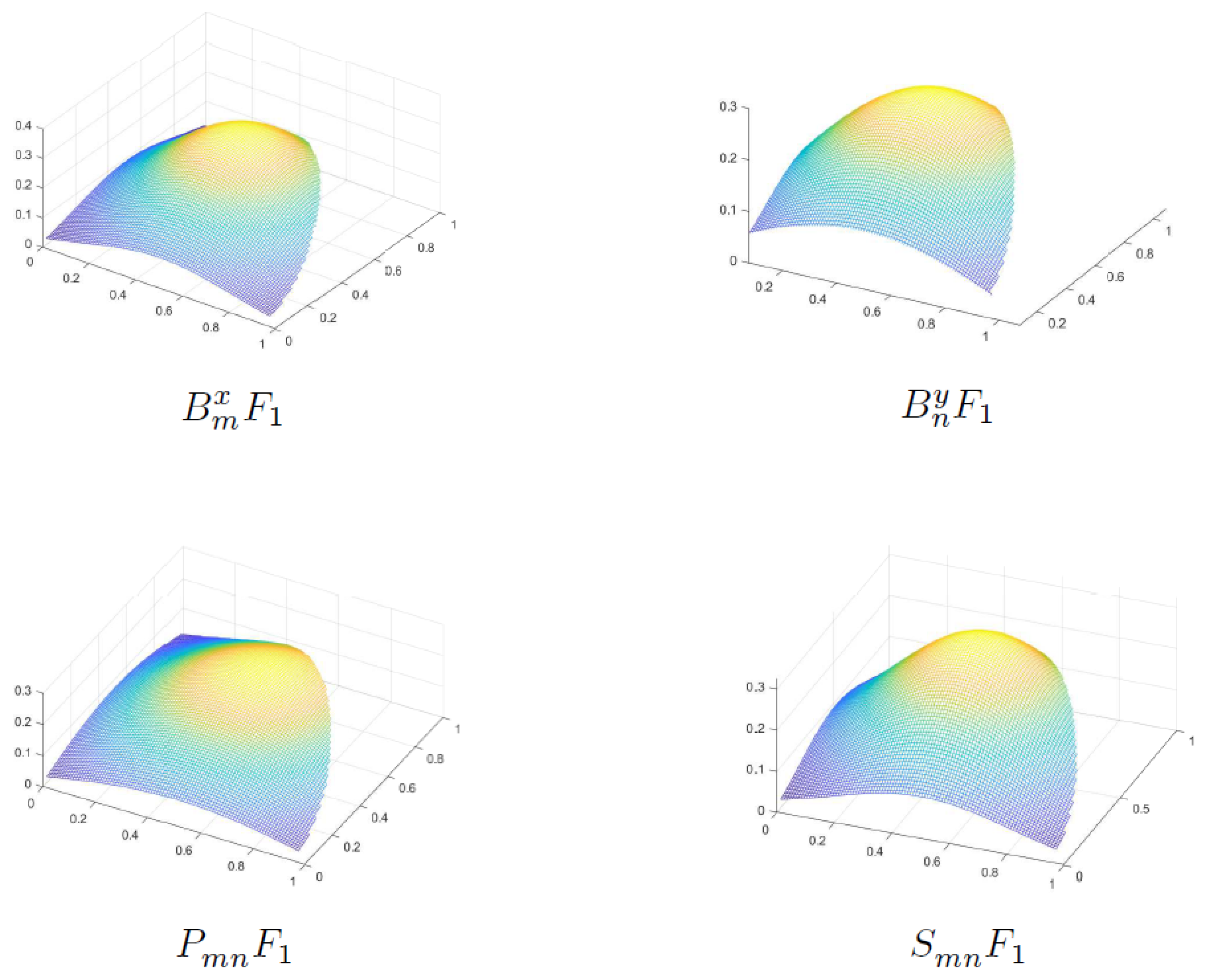
Using Matlab, in Figure 3 we plot the graphs of , defined on considering and
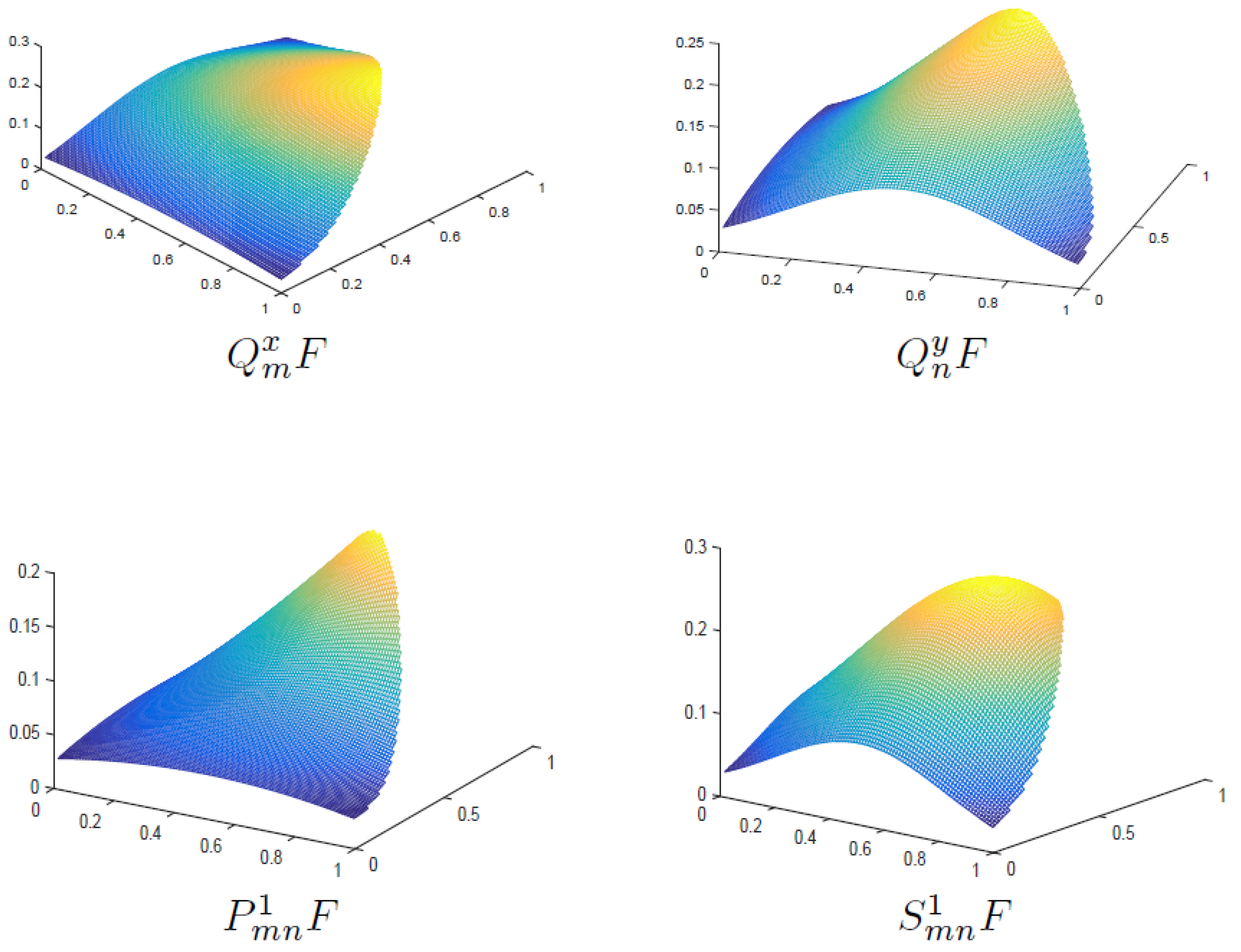
In Figure 4 we plot the graphs of , on considering ,
6. Conclusions
Funding
This research received no external funding.
Institutional Review Board Statement
Not applicable.
Informed Consent Statement
Not applicable.
Data Availability Statement
Not applicable.
Acknowledgments
We are grateful to the referees for careful reading of the manuscript and for their valuable suggestions.
Conflicts of Interest
The author declares no conflict of interest.
References
- Barnhill, R.E.; Birkhoff, G.; Gordon, W.J. Smooth interpolation in triangles. J. Approx. Theory 1973, 8, 114–128. [Google Scholar] [CrossRef]
- Barnhill, R.E.; Gregory, J.A. Polynomial interpolation to boundary data on triangles. Math. Comp. 1975, 29, 726–735. [Google Scholar] [CrossRef]
- Blaga, P.; Coman, G. Bernstein-type operators on triangle. Rev. Anal. Numer. Theor. Approx. 2009, 37, 9–21. [Google Scholar]
- Böhmer, K.; Coman, G. Blending interpolation schemes on triangle with error bounds. Lect. Notes Math. 1977, 571, 14–37. [Google Scholar]
- Cătinaş, T.; Coman, G. Some interpolation operators on a simplex domain. Stud. Univ. Babeş–Bolyai Math. 2007, 52, 25–34. [Google Scholar]
- Coman, G.; Blaga, P. Interpolation operators with applications. Sci. Math. Jpn. 2008, 68, 383–416. [Google Scholar]
- Coman, G.; Blaga, P. Interpolation operators with applications. Sci. Math. Jpn. 2009, 69, 111–152. [Google Scholar]
- Costabile, F.A.; Dell’Accio, F. Expansions over a simplex of real functions by means of Bernoulli polynomials. Numer. Algorithms 2001, 28, 63–86. [Google Scholar] [CrossRef]
- Costabile, F.A.; Dell’Accio, F. Lidstone approximation on the triangle. Appl. Numer. Math. 2005, 52, 339–361. [Google Scholar] [CrossRef]
- Nielson, G.M.; Thomas, D.H.; Wixom, J.A. Interpolation in triangles. Bull. Austral. Math. Soc. 1979, 20, 115–130. [Google Scholar] [CrossRef]
- Barnhill, R.E.; Gregory, J.A. Compatible smooth interpolation in triangles. J. Approx. Theory 1975, 15, 214–225. [Google Scholar] [CrossRef]
- Bernardi, C. Optimal finite-element interpolation on curved domains. SIAM J. Numer. Anal. 1989, 26, 1212–1240. [Google Scholar] [CrossRef]
- Blaga, P.; Cătinaş, T.; Coman, G. Bernstein-type operators on a square with one and two curved sides. Stud. Univ. Babeş-Bolyai Math. 2010, 55, 51–67. [Google Scholar]
- Blaga, P.; Cătinaş, T.; Coman, G. Bernstein-type operators on triangle with all curved sides. Appl. Math. Comput. 2011, 218, 3072–3082. [Google Scholar] [CrossRef]
- Blaga, P.; Cătinaş, T.; Coman, G. Bernstein-type operators on triangle with one curved side. Mediterr. J. Math. 2012, 9, 843–855. [Google Scholar] [CrossRef]
- Cătinaş, T. Some classes of surfaces generated by Nielson and Marshall type operators on the triangle with one curved side. Stud. Univ. Babes-Bolyai Math. 2016, 61, 305–314. [Google Scholar]
- Cătinaş, T. Extension of some particular interpolation operators to a triangle with one curved side. Appl. Math. Comput. 2017, 315, 286–297. [Google Scholar] [CrossRef]
- Cătinaş, T. Extension of Some Cheney-Sharma Type Operators to a Triangle With One Curved Side. Miskolc Math. 2020, 21, 101–111. [Google Scholar] [CrossRef]
- Cătinaş, T. Cheney-Sharma Operator on Triangle with Straight Sides. Babeş-Bolyai University, Cluj-Napoca, Romania. 2022; Unpublished work. [Google Scholar]
- Cătinaş, T.; Blaga, P.; Coman, G. Surfaces generation by blending interpolation on a triangle with one curved side. Results Math. 2013, 64, 343–355. [Google Scholar] [CrossRef]
- Coman, G.; Cătinaş, T. Interpolation operators on a tetrahedron with three curved sides. Calcolo 2010, 47, 113–128. [Google Scholar] [CrossRef]
- Coman, G.; Cătinaş, T. Interpolation operators on a triangle with one curved side. BIT Numer. Math. 2010, 50, 243–267. [Google Scholar] [CrossRef]
- Marshall, J.A.; Mitchell, A.R. An exact boundary tehnique for improved accuracy in the finite element method. J. Inst. Maths. Applics. 1973, 12, 355–362. [Google Scholar] [CrossRef]
- Mitchell, A.R.; McLeod, R. Curved elements in the finite element method. Conf. Numer. Sol. Diff. Eq. Lect. NotesIn Math. 1974, 363, 89–104. [Google Scholar]
- Barnhill, R.E. Blending function interpolation: A survey and some new results. In Numerishe Methoden der Approximationstheorie; Collatz, L., Ed.; Birkhauser-Verlag: Basel, Switzerland, 1976; Volume 30, pp. 43–89. [Google Scholar]
- Barnhill, R.E. Representation and approximation of surfaces. In Mathematical Software III; Rice, J.R., Ed.; Academic Press: New York, NY, USA, 1977; pp. 68–119. [Google Scholar]
- Barnhill, R.E.; Gregory, J.A. Sard kernels theorems on triangular domains with applications to finite element error bounds. Numer. Math. 1976, 25, 215–229. [Google Scholar] [CrossRef]
- Özger, F.; Aljimi, E.; Temizer, M. Rate of Weighted Statistical Convergence for Generalized Blending-Type Bernstein-Kantorovich Operators. Mathematics 2022, 10, 2027. [Google Scholar] [CrossRef]
- Ciarlet, P.G. The Finite Element Method for Elliptic Problems; SIAM: Philadelphia, PA, USA, 2002. [Google Scholar]
- Gordon, W.J.; Hall, C. Transfinite element methods: Blending-function interpolation over arbitrary curved element domains. Numer. Math. 1973, 21, 109–129. [Google Scholar] [CrossRef]
- Gordon, W.J.; Wixom, J.A. Pseudo-harmonic interpolation on convex domains. SIAM J. Numer. Anal. 1974, 11, 909–933. [Google Scholar] [CrossRef]
- Marshall, J.A.; Mitchell, A.R. Blending interpolants in the finite element method. Inter. J. Numer. Meth. Eng. 1978, 12, 77–83. [Google Scholar] [CrossRef]
- Dell’Accio, F.; Di Tommaso, F.; Nouisser, O.; Zerroudi, B. Increasing the approximation order of the triangular Shepard method. Appl. Numer. Math. 2018, 126, 78–91. [Google Scholar] [CrossRef]
- Dell’Accio, F.; Di Tommaso, F.; Nouisser, O.; Zerroudi, B. Fast and accurate scattered Hermite interpolation by triangular Shepard operators. J. Comput. Appl. Math. 2021, 382, 113092. [Google Scholar] [CrossRef]
- Di Tommaso, F.; Zerroudi, B. On Some Numerical Integration Formulas on the d-Dimensional Simplex. Mediterr. J. Math. 2020, 17, 142. [Google Scholar] [CrossRef]
- Cheney, E.W.; Sharma, A. On a generalization of Bernstein polynomials. Riv. Mat. Univ. Parma 1964, 5, 77–84. [Google Scholar]
- Stancu, D.D.; Cişmaşiu, C. On an approximating linear positive operator of Cheney-Sharma. Rev. Anal. Numer. Theor. Approx. 1997, 26, 221–227. [Google Scholar]
- Agratini, O. Approximation by Linear Operators; Cluj University Press: Cluj, Romania, 2000. [Google Scholar]
- Sard, A. Linear Approximation; American Mathematical Society: Providence, RI, USA, 1963. [Google Scholar]
- Renka, R.J.; Cline, A.K. A triangle-based C1 interpolation method. Rocky Mt. J. Math. 1984, 14, 223–237. [Google Scholar] [CrossRef]
Figure 1.
The standard triangle with all straight sides .

Figure 2.
The standard triangle with one curved side .

Figure 3.
The Bernstein extensions for .

Figure 4.
The Cheney–Sharma extensions for .


Table 1.
Maximum approximation errors.
| Max Error | ||
|---|---|---|
Publisher’s Note: MDPI stays neutral with regard to jurisdictional claims in published maps and institutional affiliations. |
© 2022 by the author. Licensee MDPI, Basel, Switzerland. This article is an open access article distributed under the terms and conditions of the Creative Commons Attribution (CC BY) license (https://creativecommons.org/licenses/by/4.0/).
Share and Cite
MDPI and ACS Style
Cătinaş, T. A Review on Some Linear Positive Operators Defined on Triangles. Symmetry 2022, 14, 1880. https://doi.org/10.3390/sym14091880
AMA Style
Cătinaş T. A Review on Some Linear Positive Operators Defined on Triangles. Symmetry. 2022; 14(9):1880. https://doi.org/10.3390/sym14091880
Chicago/Turabian StyleCătinaş, Teodora. 2022. "A Review on Some Linear Positive Operators Defined on Triangles" Symmetry 14, no. 9: 1880. https://doi.org/10.3390/sym14091880
Note that from the first issue of 2016, this journal uses article numbers instead of page numbers. See further details here.