Article

Modified One-Sided EWMA Charts without- and with Variable Sampling Intervals for Monitoring a Normal Process

1
School of Management, Nanjing University of Posts and Telecommunications, No. 66, Xinmofan Road, Nanjing 210003, China
2
College of Management & College of Tourism, Fujian Agriculture and Forestry University, Fuzhou 350002, China
3
School of Logistics, Wuhan University of Technology, Wuhan 430063, China
*
Author to whom correspondence should be addressed.
These authors contributed equally to this work.
Symmetry 2022, 14(1), 159; https://doi.org/10.3390/sym14010159
Submission received: 15 November 2021 / Revised: 30 December 2021 / Accepted: 9 January 2022 / Published: 13 January 2022

Abstract

:
Much research has been conducted on two-sided Exponentially Weighted Moving Average (EWMA) control charts, while less work has been devoted to the one-sided EWMA charts. Traditional one-sided EWMA charts involve resetting the EWMA statistic to the target whenever it falls below or above the target, or truncating the observations above or below the target and further applying the EWMA statistic to the truncated samples. In order to further improve the performance of traditional one-sided EWMA mean ( X ¯ ) charts, this paper studies the performance of the Modified One-sided EWMA (MOEWMA) X ¯ charts to monitor a normally distributed process. The Monte-Carlo simulation method is used to obtain the zero- and steady-state Run Length ( R L ) properties of the proposed control charts. Through extensive simulations and comparisons with other charts, it is shown that the proposed MOEWMA X ¯ charts compare favorably with some existing competing charts. Moreover, by attaching the variable sampling intervals (VSI) feature to the MOEWMA X ¯ charts, it is shown that the VSI MOEWMA charts outperform the corresponding charts without the VSI feature. Finally, a real data example from manufacturing process shows the implementation of the proposed one-sided charts.

1. Introduction

A main objective for a process is to continuously improve its quality, which can be statistically expressed as variation reduction. Chance and assignable causes exist and lead to variation in a process. The variation caused by change is unavoidable and always exists in a process, even if the operation is carried out using standardized raw material and methods. It is not practical to eliminate the chance cause technically and economically, while variation caused by assignable causes indicates that there exist some unwanted factors to be detected.
Statistical Process Monitoring (SPM) provides a large set of tools to help practitioners in monitoring manufacturing or service processes to quickly detect assignable causes. Among these, control charts are widely used online and can be implemented with a charting statistic related to the process mean or/and dispersion. The aim of a control chart is to detect abnormal changes in the process as soon as possible. Many univariate mean ( X ¯ ) charts, such as the Shewhart X ¯ chart, Cumulative Sum (CUSUM) X ¯ chart, and Exponentially Weighted Moving Average (EWMA) X ¯ chart were investigated by researchers; see Brook and Evans [1], Nelson [2], Lucas and Saccucci [3], and Hawkins and Olwell [4]. More recent works on control charts can refer to Li et al. [5], Mukherjee and Rakitzis [6], Zwetsloot et al. [7], and Perry [8], to name a few. The Shewhart charts are known to be effective when the shift size in the process is large. For the detection of small to moderate shifts, both CUSUM and EWMA charts using the current and former samples information perform much better than Shewhart type charts, see Montgomery [9].
Since the primary works of Crowder [10], Lucas and Saccucci [3], and Domangue and Patch [11], EWMA type charts have received much attention. For example, for non-normal and autocorrelated processes, the properties of EWMA X ¯ charts were first investigated by Borror et al. [12] and Lu and Jr. [13], respectively. The performance of the EWMA X ¯ chart was investigated by Jones et al. [14] when the process parameters are estimated. Recently, Celano et al. [15], Calzada and Scariano [16], and Haq et al. [17] studied the run length performance of the EWMA t charts. To summarise, only a two-sided EWMA chart was used in the above researches. In practice, the direction of the out-of-control shift is usually known in advance, which implies that it is possible to tune the upward and downward parts of EWMA charts separately [18]. Then two separate one-sided EWMA charts were studied by some researchers. For instance, Tran et al. [19] and Tran and Knoth [20] studied the properties of two one-sided EWMA charts to monitor the ratio of two variables. Zhang et al. [21] and Muhammad et al. [22] investigated the performance of two one-sided EWMA charts for monitoring the coefficient of variation (CV).
In this paper, the work in Zhang et al. [21] is highlighted for the new resetting model of the Modified One-sided EWMA (MOEWMA) charting statistic. In the EWMA charting statistic, information of former and current samples are both used and the charting statistic is reset to the target if it is smaller than the target. While their work studied the EWMA chart for monitoring the CV, as far as we know, there is no research on the proposed scheme for monitoring the mean of a normally distributed process. In fact, a normally distributed quality characteristic usually exists in some industrial processes. To fill this gap, we investigate the properties of the MOEWMA X ¯ charts. In addition, it is known that control charts with the variable sampling interval (VSI) features are more efficient than the corresponding fixed sampling interval (FSI) charts in the detection of shifts. In the past decades, much research has been conducted on VSI control charts. For instance, Nguyen et al. [23] suggested a VSI CUSUM chart to monitor the ratio of two normal variables and showed that the proposed chart had some advantages over the corresponding FSI CUSUM chart. Using extensive Monte-Carlo simulations, Haq [24] studied the performance of the weighted adaptive multivariate CUSUM chart with VSI feature. It was shown that the proposed charts perform uniformly better than the corresponding FSI charts in terms of the ATS (Average Time to Signal) and AATS (Average Adjusted Time to Signal) performances. Coelho et al. [25] proposed a VSI nonparametric Shewhart type control chart, which was shown to be better than the existing FSI chart. For more research works, we direct readers to the works [26,27,28,29,30,31] and the references cited therein. To further increase the sensitivity of the MOEWMA X ¯ charts and gain motivation from the above works on the VSI charts, the VSI MOEWMA X ¯ charts are proposed, and it is expected that the VSI MOEWMA charts perform better than the corresponding FSI one-sided charts.
The remainder of this paper is organized as follows: Section 2 reviews several types of one-sided EWMA X ¯ charts and presents the MOEWMA X ¯ chart. The zero-state (ZS) and steady-state (SS) Average Run Length ( A R L ) performances of the proposed MOEWMA X ¯ charts are presented in Section 3 and are compared with other competing charts. Section 4 presents the detailed construction of the MOEWMA X ¯ charts with the VSI feature and, moreover, both the ZS and SS performances of the proposed VSI MOEWMA X ¯ charts are investigated. A real data example is used to illustrate the implementation of the MOEWMA X ¯ charts in Section 5. Finally, some conclusions and recommendations are made in the last section.

2. One-Sided EWMA Type Charts

Assume that { X t , 1 , , X t , n } , t = 1 , 2 , is a sample of size n 1 from an independent normal distribution, i.e., X t N ( μ 0 + δ σ 0 , σ 0 ) , where μ 0 and σ 0 are the in-control mean and standard deviation, respectively, and δ is the magnitude of the mean shift. When δ = 0 , the process is considered to be in-control. Otherwise, the process is out-of-control. At each sample point t = 1 , 2 , , the sample mean X ¯ t = 1 n j = 1 n X t , j is computed for the process monitoring, where X ¯ t N ( μ 0 + δ σ 0 , σ 0 n ) . Without loss of generality, we assume μ 0 = 0 and σ 0 = 1 in this paper.

2.1. Traditional One-Sided EWMA Charts

The traditional two-sided EWMA X ¯ chart construct the monitoring statistic Z t = λ X t ¯ + ( 1 λ ) Z t 1 , t = 1 , 2 , 3 , , with a fixed smoothing constant λ ( 0 , 1 ] and the initial value Z 0 = μ 0 . The upper ( U C L ) and lower ( L C L ) control limits of the EWMA X ¯ chart are generally selected based on the constraint of the desired in-control A R L . If Z t [ L C L , U C L ] , the process is considered to be in-control. Otherwise, if Z t [ L C L , U C L ] , the process is deemed to be out-of-control. Instead of using a single two-sided EWMA X ¯ chart, when the direction of the shift is known, three types of one-sided EWMA X ¯ charts were suggested by some researchers. These charts are summarized as follows:
(1)
A simple use of the one-sided EWMA X ¯ chart is to set only an upper control limit ( U C L ) or a lower control limit ( L C L ) with the traditional charting statistic Z t = λ X t ¯ + ( 1 λ ) Z t 1 and the initial value Z 0 = μ 0 . This chart is denoted as SEWMA X ¯ chart. That is to say, the upper-sided SEWMA X ¯ chart declares an alarm when Z t > U C L and the lower-sided SEWMA X ¯ chart declares an alarm when Z t < L C L . More details of the SEWMA X ¯ chart can be seen in Robinson and Ho [32].
(2)
A second use of the one-sided EWMA X ¯ chart is to reset the traditional EWMA statistic to the target whenever it is smaller than the target (for the upper-sided chart) or whenever it is larger than the target (for the lower-sided chart). This chart is denoted as REWMA X ¯ chart. The charting statistics Z t + and Z t of the upper- and lower-sided REWMA X ¯ charts are given as follows,
Z t + = max ( μ 0 , λ X t ¯ + ( 1 λ ) Z t 1 + ) ,
and
Z t = min ( μ 0 , λ X t ¯ + ( 1 λ ) Z t 1 ) .
with the initial value Z 0 = μ 0 . An out-of-control signal is triggered as soon as Z t + > U C L (for the upper-sided REWMA X ¯ chart) or Z t < L C L (for the lower-sided REWMA X ¯ chart), respectively. More details of REWMA type charts can be seen in Hamilton and Crowder [33] and Gan [34].
(3)
A third use of the one-sided EWMA X ¯ chart is first truncate the sample mean X ¯ t below the target to the target value (for the upper-sided chart) or above the target to the target value (for the lower-sided chart), and then apply the EWMA recursion to these truncated values. This chart is denoted as IEWMA X ¯ chart. The charting statistic Z t of the IEWMA chart is given as follows:
Z t = λ W t + ( 1 λ ) Z t 1 ,
where W t = W t ( μ 0 + 1 / 2 π σ 0 ) / n σ 0 0.5 0.5 / π / n is the standardized value of W t = max ( μ 0 , X t ¯ ) (for the upper-sided chart), and W t = W t ( μ 0 1 / 2 π σ 0 ) / n σ 0 0.5 0.5 / π / n is the standardized value of W t = min( μ 0 , X t ¯ ) (for the lower-sided chart). The initial value Z 0 is set as 0. An out-of-control signal is given when Z t > U C L in the upper-sided chart or Z t < L C L in the lower-sided chart. More details of this chart can be seen in Shu and Jiang [35] and Shu et al. [36].

2.2. The Proposed MOEWMA X ¯ Charts

In this section, the MOEWMA X ¯ charts with a new resetting model are investigated. As it will be shown in Section 3, the proposed charts outperform the traditional one-sided EWMA X ¯ charts presented in Section 2.1.
It can be seen from Equation (1) that, when λ X ¯ t + ( 1 λ ) Z t 1 + is smaller than μ 0 , then Z t + = μ 0 and Z t + 1 + = max ( μ 0 , λ X ¯ t + 1 + ( 1 λ ) μ 0 ) . All the samples information collected before time t + 1 are lost. As the main advantage of EWMA type charts is to use both current and former samples information, the charting statistic of the upper-sided MOEWMA X ¯ chart is constructed as,
Z t + = max ( μ 0 , λ X ¯ t + ( 1 λ ) Z t 1 ) ,
where Z t 1 = λ X ¯ t 1 + ( 1 λ ) Z t 2 and the initial value Z 0 = μ 0 . It can be noted that the charting statistic Z t + in Equation (4) uses all samples information collected before. The chart triggers an out-of-control signal if Z t + is larger than the U C L . Similarly, a lower-sided MOEWMA X ¯ is suggested with the following charting statistic,
Z t = min ( μ 0 , λ X ¯ t + ( 1 λ ) Z t 1 ) ,
where the initial value Z 0 = μ 0 . An out-of-control signal is triggered if Z t is smaller than the L C L .

3. Numerical Results and Comparisons

In this section, some R L measures, including the A R L and the Standard Deviation of Run Length ( S D R L ) are used to investigate the performance of the one-sided EWMA charts in Section 2. The A R L is defined as the expected number of samples on the chart until a signal occurs. A control chart is desirable when the in-control A R L is large and at the same time, the out-of-control A R L is as small as possible. In addition, the S D R L determines the variability of the R L distribution. The smaller the S D R L value, the better the A R L performance of a control chart, see Haq [37]. In addition, the subscripts 0 and 1 are used with A R L and S D R L to denote the in-control and out-of-control properties, respectively. To obtain these R L properties of the proposed chart, the Monte-Carlo method is adopted in this paper. Under each simulation run, 10 5 iterations of R L values are used to calculate the values of A R L and S D R L .

3.1. Comparisons with Some Competing Charts

In this section, to provide some direct insight into the performance of the proposed charts, the ( A R L , S D R L ) of the MOEWMA X ¯ charts are compared with the ones of the SEWMA, REWMA, and IEWMA X ¯ charts. The properties of the SEWMA, REWMA, and IEWMA X ¯ charts can be obtained using the Markov chain approach. For the EWMA type charts, values of 0.05 λ 0.25 were recommended by Montgomery [9]. Moreover, a relatively small smoothing parameter λ is usually suggested for monitoring small shifts while larger values of λ are suggested for larger shifts. In this paper, λ { 0.05 , 0.1 , 0.2 , 0.25 } are selected for illustration and the corresponding control limits of EWMA type charts can be obtained with the constraint on the desired A R L 0 . For simplicity, the A R L 0 is set to be 200. For the proposed one-sided MOEWMA X ¯ chart, a bisection algorithm similar to Dickinson et al. [38] is used to find the control limit. The algorithm stops when the in-control A R L falls within the interval [ A R L 0 1 , A R L 0 + 1 ] .
Table 1 presents the ( A R L 1 , S D R L 1 ) values of these EWMA control charts for different shifts δ varying from 0.1 to 3 when n { 3 , 5 } . It can be noted from this table that, for the upper-sided MOEWMA X ¯ chart, a small value of λ is relatively effective for small shifts δ and vice verse. For instance, when n = 3 and δ = 0.1 , the ( A R L 1 , S D R L 1 ) = (54.06, 45.94) of the upper-sided MOEWMA X ¯ chart when λ = 0.05 is smaller than the ( A R L 1 , S D R L 1 ) = (75.26, 71.98) of the chart when λ = 0.25 . Compared with the competing EWMA (SEWMA, REWMA, and IEWMA) charts, some conclusions are made as follows:
  • Irrespective of the values of δ and n, the A R L 1 and S D R L 1 values of the upper-sided MOEWMA X ¯ chart are generally smaller than the ones of the upper-sided REWMA X ¯ chart, especially for small shifts. This fact clearly demonstrates the advantage of the proposed chart. For instance, when n = 3 , λ = 0.1 , and δ = 0.1 , the ( A R L 1 , S D R L 1 ) = ( 60.12 , 54.07 ) of the upper-sided MOEWMA X ¯ chart are smaller than the ( A R L 1 , S D R L 1 ) = ( 70.17 , 62.84 ) of the upper-sided REWMA X ¯ chart.
  • The proposed chart always has a little smaller A R L 1 value than the one of the upper-sided SEWMA X ¯ chart. For example, for the same values of n, λ and δ presented above, the ( A R L 1 , S D R L 1 ) = ( 61.11 , 54.11 ) of the upper-sided SEWMA X ¯ chart are close to the ones of the upper-sided MOEWMA X ¯ chart.
  • Compared with the upper-sided IEWMA X ¯ chart, the proposed chart performs better for small shifts and worse for moderate to large shifts. For instance, when n = 3 and λ = 0.1 , the upper-sided MOEWMA X ¯ chart with ( A R L 1 , S D R L 1 ) = (60.12, 54.07) is better than the upper-sided IEWMA X ¯ chart with ( A R L 1 , S D R L 1 ) = (68.17, 63.64) for the detection of δ = 0.1 . However, for the detection of δ = 1 , the upper-sided MOEWMA chart with ( A R L 1 , S D R L 1 ) = (3.81, 1.29) is worse than the upper-sided IEWMA chart with ( A R L 1 , S D R L 1 ) = (3.38, 1.43).
  • For a large shift, for instance when δ = 3 or larger than 3, all the charts perform similarly, as the A R L 1 is close to 1 and the S D R L 1 value converges to 0 with δ increasing.
As the symmetry of the normal distribution, similar conclusions are drawn for the lower-sided MOEWMA X ¯ chart. For simplicity, these results are not presented here.

3.2. Optimal Performance of the Proposed MOEWMA X ¯ Charts

The results in Section 3.1 show the advantage of the proposed chart over the SEWMA, REWMA, and IEWMA X ¯ charts. All of the simulations above are for a fixed value of λ , which is not optimal for the specified shift size δ o p t . To provide a fare comparison, the optimal performances of different charts for the intended shift size are compared in this section. The optimal design of the upper-sided MOEWMA X ¯ chart involves determining the chart parameters ( λ , U C L ) to minimize the A R L 1 at a specified mean shift δ o p t , at the same time, satisfying the constraint on the desired A R L 0 . The procedure can be concluded as a constrained nonlinear minimization problem:
( λ * , U C L * ) = argmin ( λ , U C L ) A R L 1 ( n , λ , U C L , δ o p t ) ,
subject to
A R L ( n , λ , U C L , δ = 0 ) = A R L 0 .
By using this model, extensive computation works are then performed to numerically find the nearly optimal parameters ( λ * , U C L * ) of the upper-sided MOEWMA X ¯ chart. Table 2 presents the optimal chart parameters ( λ * , U C L * ) of the proposed chart for δ o p t and the ( A R L 1 , S D R L 1 ) values of the chart at shift δ varying from 0.1 to 3. As a comparison, the nearly optimal parameters and performances of the REWMA, SEWMA, and IEWMA X ¯ charts are also presented. All charts are designed to maintain A R L 0 = 200 . For example, if the specified shift size δ o p t = 0.3 , the U C L s of the upper-sided MOEWMA X ¯ chart are first determined for λ { 0.05 , 0.06 , . . . , 0.99 , 1 } to obtain A R L 0 = 200 . The A R L 1 values are then computed for all the combinations of ( λ , U C L ) . The parameters ( λ * , U C L * ) = ( 0.05 , 0.17 ) leading to the smallest A R L 1 = 15.79 are considered to be the nearly optimal parameters of the control chart.
It can be concluded from Table 2 that:
  • If the specified shift is small ( δ o p t 0.5 ), the optimal upper-sided MOEWMA X ¯ chart performs better than the optimal REWMA, SEWMA, and IEWMA X ¯ charts. For instance, if δ o p t = 0.3 , the optimal parameters ( λ * , U C L * ) of the upper-sided MOEWMA X ¯ chart is (0.05, 0.17) and the corresponding ( A R L 1 , S D R L 1 ) = ( 15.79 , 9.27 ) is the smallest one among these charts.
  • The upper-sided MOEWMA X ¯ chart provides a good sensitivity against shifts smaller than the specified δ o p t and the upper-sided IEWMA X ¯ chart performs better than other charts for shifts larger than the specified δ o p t . For instance, if δ o p t = 0.3 , while the actual shift size in the process is not the specified one and is δ = 0.1 (smaller than δ o p t = 0.3 ), the upper-sided MOEWMA X ¯ chart with ( A R L 1 , S D R L 1 ) = ( 53.80 , 45.49 ) is better than other charts. If the actual shift size is δ = 1 (larger than δ o p t = 0.3 ), the upper-sided IEWMA X ¯ chart with ( A R L 1 , S D R L 1 ) = ( 3.61 , 1.41 ) performs better than other charts.
  • If the specified shift is moderate ( 1 < δ o p t 2 ), the upper-sided IEWMA X ¯ chart has better sensitivity than the REWMA, SEWMA, and MOEWMA X ¯ charts for all the shift sizes. For example, when δ o p t = 1.5 , the optimal ( A R L 1 , S D R L 1 ) = (1.74, 0.87) of the upper-sided IEWMA X ¯ chart is smaller than the ones of these charts, and if the actual shift sizes is smaller or larger than 1.5, the upper-sided IEWMA X ¯ chart still performs better than these charts.
  • If the actual shift size is large ( δ o p t 2.5 ), the upper-sided MOEWMA X ¯ chart has the best performance among all the charts. For instance, when δ o p t = 3 , the optimal ( A R L 1 , S D R L 1 ) = ( 1.00 , 0.07 ) is the same for all the charts. If the actual shift size is smaller than δ o p t = 3 , it can be seen that the upper-sided MOEWMA X ¯ chart has the smallest ( A R L 1 , S D R L 1 ) value among these EWMA type charts.
The above results also indicate that both the upper-sided IEWMA and MOEWMA X ¯ charts have a practical property of good performance over a wide range of shifts rather than a scheme to optimize the control charts at a specified shift δ o p t . This property was considered to be important, as in applications, the value of shift size is seldom known, and therefore a robust monitoring procedure that efficiently signals a range of shifts is useful [39].

3.3. The Steady-State Performance of the Proposed Chart

The results presented in the previous section are for the case in which the shift occurs from the beginning of the process or the charting statistic is at its initial starting value when the shift occurs. The computed A R L in this way is referred as the zero-state A R L . The steady-state A R L is based on the assumption that the process remains in-control for a long time and a shift occurs later in the process. The steady-state A R L of control chart is considered to be more realistic than the zero-state A R L , see Zwetsloot et al. [7]. For the steady-state case, 10 5 Monte-Carlo simulations are used to estimate the steady-state A R L values of control charts and the shift is assumed to happen in the process after 50 in-control samples, see Dickinson et al. [38], Xu and Jeske [40], and Haq [24].
The out-of-control steady-state A R L 1 and S D R L 1 of the proposed chart together with the ones of the REWMA, SEWMA, and IEWMA X ¯ charts are presented in Table 3 for different combinations of n, λ , and δ . The in-control A R L 0 is set to be 200. It can be noted from Table 3 that the steady-state performance of the upper-sided MOEWMA X ¯ chart is almost the same as the upper-sided SEWMA X ¯ chart. Moreover, for a small shift ( δ 0.3 ), both the upper-sided MOEWMA X ¯ chart and the upper-sided SEWMA X ¯ chart generally perform better than the upper-sided IEWMA and REWMA X ¯ charts. For instance, when n = 3 , λ = 0.1 , and δ = 0.1 , the steady-state ( A R L 1 , S D R L 1 ) = (58.66, 54.58) and ( A R L 1 , S D R L 1 ) = (58.63, 54.38) of the upper-sided SEWMA and MOEWMA X ¯ charts are smaller than the steady-state ( A R L 1 , S D R L 1 ) = (67.22, 63.92) and ( A R L 1 , S D R L 1 ) = (65.35, 62.84) of the upper-sided IEWMA and REWMA X ¯ charts. Moreover, for the shifts larger than 0.5, we can note that the upper-sided IEWMA X ¯ chart generally performs best among these charts. The upper-sided REWMA X ¯ chart is preferred only when δ = 0.5 .

4. MOEWMA X ¯ Charts with Variable Sampling Intervals

4.1. Construction of the VSI MOEWMA X ¯ Charts

The MOEWMA X ¯ charts studied above are FSI type charts, which fixes the time intervals between samples. As suggested by Reynolds et al. [41], X ¯ chart with VSI features performed better than the corresponding FSI chart. The VSI feature allows a chart to vary the time intervals between samples depending on the value of the charting statistic. For the one-sided type charts, by adding an upper warning limit ( U W L ) of the upper-sided chart (or a lower warning limit ( L W L ) of the lower-sided chart), the in-control region of one-sided control charts are divided into a warning region and a central region. If the value of the charting statistic falls in the warning region, it is suspected that the process is at risk and the next sample should be taken after a short sampling interval h S . If the value of the charting statistic falls in the central region, the process is deemed to be safe and the next sample could be taken after a long sampling interval h L . Otherwise, the process is considered to be out-of-control when the value of the charting statistic falls outside the U C L the upper-sided chart (or the L C L of the lower-sided chart).
Let U W L and L W L be the warning limits of the upper-sided and lower-sided VSI MOEWMA X ¯ chart, respectively, and h t { h S , h L } be the sampling interval between the tth and ( t + 1 ) th samples. The central regions of the upper-sided and lower-sided MOEWMA X ¯ charts are [0, U W L ] and [ L W L , 0], respectively. The warning regions of the upper-sided and lower-sided MOEWMA X ¯ charts are ( U W L , U C L ] and [ L C L , L W L ), respectively. For the upper-sided VSI MOEWMA X ¯ chart, h t switches as follows:
h t = h S , Z t + [ 0 , U W L ] , h L , Z t + ( U W L , U C L ] .
where Z t + is defined in Equation (4). Similarly, the h t of the lower-sided VSI MOEWMA X ¯ chart depends on the value of the Z t defined in Equation (5). Thus, for the VSI MOEWMA X ¯ chart, the sampling intervals h t varies as a function of the charting statistic Z t + (for the upper-sided chart) or Z t (for the lower-sided chart).
When the process monitoring starts at time 0, no sample information is available to select the value of h 0 . It might be practical to use the short sampling interval h 0 = h S to protect against problems in the start-up period [41]. As suggested by Reynolds et al. [42], when the process is in-control, the values of sampling intervals h S and h L are obtained by satisfying the following constraints,
ρ 1 h S + ρ 2 h L = 1 , ρ 1 + ρ 2 = 1 ,
where ρ 1 and ρ 2 are the long run proportions of sampling intervals that are h S and h L , respectively. In addition, it is noted that the charting statistics in Equation (4) is reset to 0 if it is smaller than 0. This causes the fact that nearly half values of the in-control charting statistics are always 0 and are in the safe region and the sampling interval corresponding to these values is h L . By doing many simulations, it is then found that the value of ρ 1 and ρ 2 are always smaller and larger than 0.5, respectively. For illustration, ρ 1 = 0.4 , ρ 2 = 0.6, and ( h S , h L ) = ( 0.1 , 1.6 ) are selected in this paper. It is noted that the value of h S may be practically determined by the minimum time required to take a sample and h L should not exceed the maximum time to allow the process to run without sampling. In addition, the values of ρ 1 , ρ 2 and ( h S , h L ) should satisfy the constraint in Equation (7). For simplicity, the VSI MOEWMA X ¯ chart’s performance for other combination of ρ 1 , ρ 2 , and ( h S , h L ) are not presented in this manuscript.

4.2. Comparison with the FSI MOEWMA X ¯ Charts

It is well known that the A T S , instead of A R L , was usually suggested to evaluate a VSI chart’s performance. For an FSI chart, the A T S is a constant multiple of the A R L , while for a VSI chart, the A T S is no longer a constant multiple of the A R L due to the varying of sampling intervals. In this case, the A T S is defined as the expected time from the start of the process to an out-of-control signal. Similarly, if the process has been running for a long time so the EWMA statistic is in a steady-state before the shift happens, the adjusted A T S ( A A T S ) is usually used to evaluate the properties of a VSI chart, see Reynolds et al. [42]. In this paper, both A T S and A A T S are used together to compare the performances of the FSI and VSI MOEWMA X ¯ charts. The Monte-Carlo method is also used to obtain the A T S and A A T S of the VSI MOEWMA X ¯ chart. The simulation settings of the VSI MOEWMA X ¯ chart is similar to those of the FSI MOEWMA charts in Section 3.3.
Table 4 and Table 5 present the out-of-control A T S and A A T S of the FSI and VSI MOEWMA X ¯ charts for different values of λ and δ when n { 3 , 5 } . In addition, the subscripts 0 and 1 are used with A T S and A A T S to denote the in-control and out-of-control properties of the VSI chart, respectively. For fair comparisons, the desired in-control A T S 0 of both charts are matched as 200.
From these tables, it can be concluded that whether in the zero-state or steady-state, for fixed values of n, λ and δ , the VSI MOEWMA X ¯ chart has smaller A T S 1 or A A T S 1 values than the those of the corresponding FSI chart. This fact indicates that the VSI MOEWMA X ¯ chart is substantially better than the FSI MOEWMA X ¯ chart. For example, for the zero-state case in Table 4, when n = 3 and λ = 0.1 , the A T S 1 = 40.62 of the VSI MOEWMA X ¯ chart is smaller than the A T S 1 = 60.12 of the FSI MOEWMA X ¯ chart for δ = 0.1 . In addition, the VSI MOEWMA X ¯ chart with a small λ performs better than the chart with a large λ to detect small shifts in the process and viceversa. For example, if the specified shift δ = 0.1 , the A T S 1 = 32.52 of the VSI MOEWMA X ¯ chart with λ = 0.05 performs better than the A T S 1 = 57.46 of the chart with λ = 0.25 . Furthermore, if the specified shift δ = 2.0 , the A T S 1 = 0.22 of the VSI MOEWMA X ¯ chart with λ = 0.05 is worse than the A T S 1 = 0.16 of the chart with λ = 0.25 . As the A T S 1 or A A T S 1 values are close to 0 for large shifts, the VSI MOEWMA X ¯ chart with a smaller λ is generally recommended in practice. Moreover, for fixed values of n, λ , and δ , the A A T S 1 value of the VSI MOEWMA X ¯ chart is larger than the A T S 1 of the chart. For example, when n = 3 , λ = 0.1 , and δ = 0.1 , the A A T S 1 = 47.35 (see Table 5) of the chart is larger than the A T S 1 = 40.62 (see Table 4).

5. A Real Data Application

To show the application of the REWMA, SEWMA, IEWMA, and the proposed MOEWMA X ¯ charts, in what follows, a real dataset of semiconductor manufacturing in Montgomery [9] is used to illustrate the charts’ implementation. The photolithography process is important in semiconductor manufacturing. It transfers a geometric pattern from a mask to the surface of a silicon wafer using light-sensitive photoresist materials. This process is complex as it involves many engineering steps, for instance, chemical cleaning of the wafers, formation of barrier layer using silicon dioxide, and hard-baking process to increase photoresist adherence to the wafer surface. During the hard-baking process, the flow width of the photoresist is an important quality characteristic that needs to be monitored, as a minor variation (10 nm) in the thickness of photoresist will change the interference color and discolor the photoresist film.
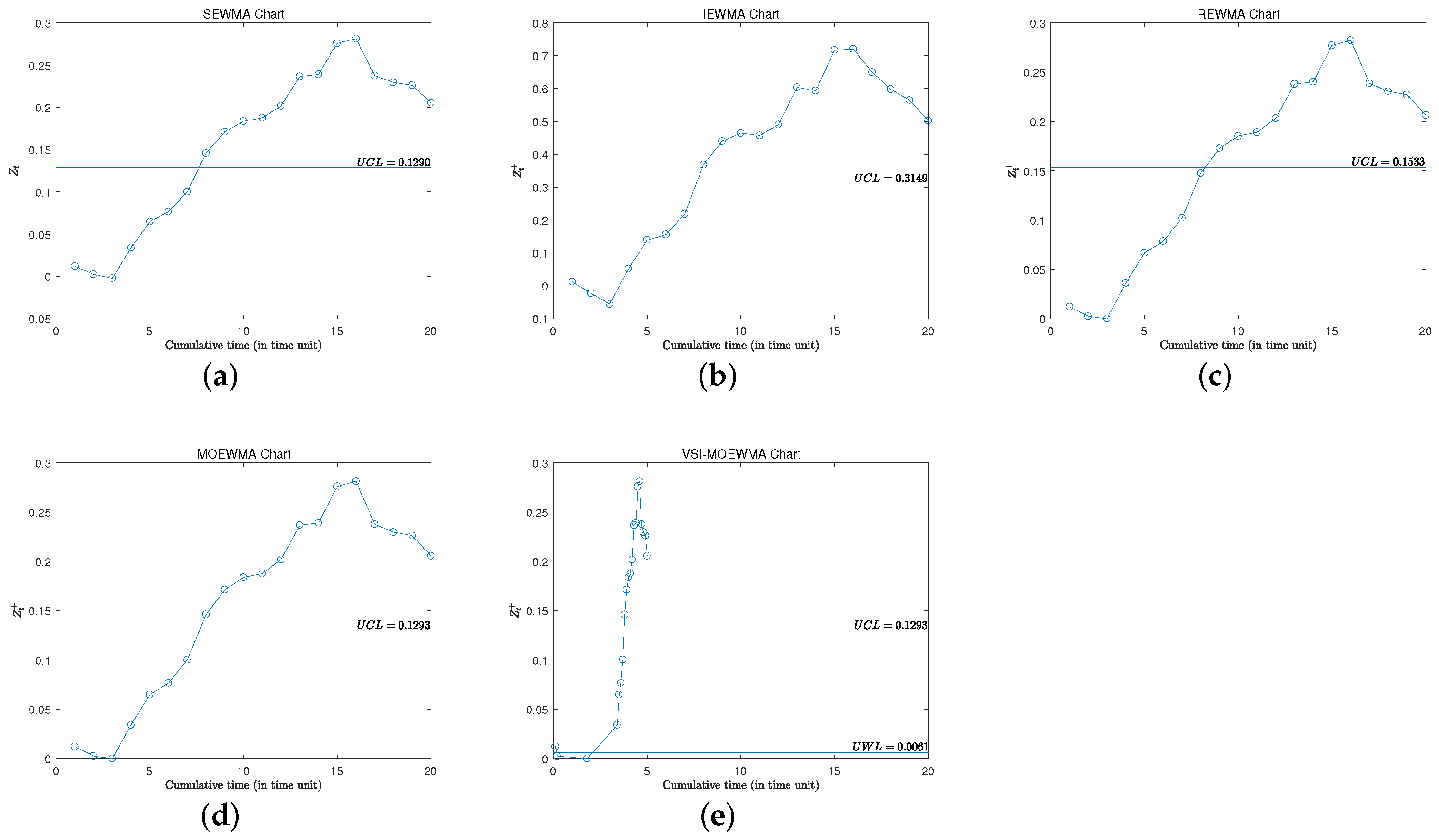
Suppose that flow width can be controlled at a mean μ 0 = 1.5 microns and the standard deviation σ 0 = 0.15 microns of a normally distributed process and the quality practitioner anticipates an upward shift size δ = 0.3 in the process when the process is out-of-control. Then the upper-sided MOEWMA X ¯ chart is implemented for the process monitoring at each sampling point. For the FSI (VSI) chart, the desired A R L 0 ( A T S 0 ) is maintained as 200, and ( h S , h L ) = (0.1, 1.6) are selected.
In Table 6, 20 samples, each with size n = 5 , are generated from an out-of-control normal distribution of the flow width with the mean μ 1 = μ 0 + δ × σ 0 = 1.5 + 0.3 × 0.15 = 1.545 and the standard deviation σ 0 . All sample mean values { X ¯ 1 , X ¯ 2 , , X ¯ 20 } and the corresponding values of the different EWMA charting statistics are listed in the table. As a comparison, the upper-sided SEWMA, REWMA, and IEWMA X ¯ charts together with the MOEWMA X ¯ chart are plotted in Figure 1. It can be noted from Figure 1 that all control charts give an out-of-control signal at the 8th sample point, except for the upper-sided REWMA X ¯ chart, where the chart gives an out-of-control signal at the 9th sample point (see the bolded values in Table 6). This example shows that these FSI EWMA charts take about 8 or 9 time units to detect the assignable cause while, on average, we can note from Table 1 that the MOEWMA chart detect the shift δ = 0.3 more quick than the SEWMA, REWMA, and IEWMA X ¯ charts.
Moreover, for the VSI-MOEWMA chart, the charting statistics Z 2 + and Z 3 + fall in the central region [0, U W L ], which leads to a large sampling interval h L = 1.6 to find the subsequent samples. For the charting statistic at other sampling time point, the corresponding sampling interval is h S = 0.1 . This leads to a A T S 1 = 3.8 time unit of the VSI-MOEWMA X ¯ chart to detect the assignable cause. Thus, it is better to adopt the VSI-MOEWMA X ¯ chart to monitor the process.

6. Conclusions and Recommendations

In this paper, we study the performance of one-sided MOEWMA X ¯ chart without- and with VSI features. Both the zero-state and steady-state performances of the FSI and VSI MOEWMA X ¯ chart are investigated by using extensive Monte-Carlo simulations. Through a comprehensive comparison with the SEWMA, REWMA, and IEWMA X ¯ charts, it is found that the MOEWMA X ¯ chart is shown to perform better than the REWMA X ¯ chart, especially for small shifts and it performs better than the IEWMA X ¯ chart for small shifts and worse for moderate to large shifts. Moreover, the MOEWMA X ¯ chart is always a little better than the SEWMA X ¯ chart. In addition, by investigating the optimal performance of the MOEWMA X ¯ chart, it can be concluded that the optimal MOEWMA X ¯ chart has a good performance over a wide range of shifts rather than a scheme to optimize the control charts at a specified shift. Finally, by adding the VSI feature to the MOEWMA X ¯ chart, it is shown that the VSI MOEWMA X ¯ chart is uniformly better than its counterpart with FSI, especially for small shifts.
As the current research works are based on the assumption of known process parameters, the manner in which the control chart performs with estimated process parameters remains an issue. Future works could be extended to this aspect. Moreover, this research is focused on the monitoring of the process mean. The methodology can also be extended to monitor the process variance, the ratio of two distributions, and so on.

Author Contributions

Conceptualization, X.H. and S.Z.; methodology, X.H.; software, S.Z.; validation, X.H., S.Z. and G.S.; formal analysis, G.S.; investigation, J.Z.; resources, S.W.; data curation, S.W.; writing—original draft preparation, S.Z. and G.S.; writing—review and editing, X.H. and J.Z.; visualization, S.W.; supervision, X.H.; project administration, X.H.; funding acquisition, X.H. All authors have read and agreed to the published version of the manuscript.

Funding

This research was funded by National Natural Science Foundation of China grant number 71802110, 71801049, 11701437 and Key Research Base of Philosophy and Social Sciences in Jiangsu-Information Industry Integration Innovation and Emergency Management Research Center and the Excellent Innovation Teams of Philosophy and Social Science in Jiangsu Province grant number 2017ZSTD022 and Postgraduate Research and Practice Innovation Program of Jiangsu Province grant number KYCX21_0840.

Institutional Review Board Statement

Not applicable.

Informed Consent Statement

Not applicable.

Data Availability Statement

All relevant data are within the manuscript.

Acknowledgments

The authors would like to express appreciation to Fupeng Xie from Nanjing University of Science and Technology for his works on Software.

Conflicts of Interest

The authors declare no conflict of interest.

Abbreviations

The following abbreviations are used in this manuscript:
EWMAExponentially Weighted Moving Average
CUSUMCumulative Sum
MOEWMAModified One-sided EWMA
SEWMAThe simple one-sided EWMA chart
REWMAEWMA chart with resetting the charting statistic to the target
IEWMAEWMA chart with truncating the sample mean to the target
RLRun Length
ARLAverage Run Length
A R L 0 In-control ARL
A R L 1 Out-of-control ARL
SDRLStandard Deviation of Run Length
S D R L 0 In-control SDRL
S D R L 1 Out-of-control SDRL
ATSAverage Time to Signal
A T S 0 In-control ATS
A T S 1 Out-of-control ATS
AATSAverage Adjusted Time to Signal
A A T S 0 In-control AATS
A A T S 1 Out-of-control AATS
VSIVariable Sampling Interval
FSIFixed Sampling Interval
UCLUpper Control Limit
LCLLower Control Limit
UWLUpper Warning Limit
LWLLower Warning Limit
ZSZero-State
SSSteady-State

References

  1. Brook, D.; Evans, D. An Approach to the Probability Distribution of CUSUM Run Length. Biometrika 1972, 59, 539–549. [Google Scholar] [CrossRef]
  2. Nelson, L. The Shewhart Control Chart–Tests for Special Causes. J. Qual. Technol. 1984, 16, 237–239. [Google Scholar] [CrossRef]
  3. Lucas, J.; Saccucci, M. Exponentially weighted moving average control schemes: Properties and enhancements. J. Qual. Technol. 1990, 32, 1–12. [Google Scholar]
  4. Hawkins, D.; Olwell, D. Cumulative Sum Charts and Charting for Quality Improvement; Springer: New York, NY, USA, 1999. [Google Scholar]
  5. Li, Z.; Zou, C.; Gong, Z.; Wang, Z. The computation of average run length and average time to signal: An overview. J. Stat. Comput. Simul. 2014, 84, 1779–1802. [Google Scholar] [CrossRef]
  6. Mukherjee, A.; Rakitzis, A.C. Some simultaneous progressive monitoring schemes for the two parameters of a zero-inflated Poisson process under unknown shifts. J. Qual. Technol. 2019, 51, 257–283. [Google Scholar] [CrossRef]
  7. Zwetsloot, I.M.; Mahmood, T.; Woodall, W.H. Multivariate Time-Between-Events Monitoring–An overview and some (overlooked) underlying complexities. Qual. Eng. 2020, 33, 13–25. [Google Scholar] [CrossRef]
  8. Perry, M.B. An EWMA control chart for categorical processes with applications to social network monitoring. J. Qual. Technol. 2020, 52, 182–197. [Google Scholar] [CrossRef]
  9. Montgomery, D.C. Intorduction to Ststistical Quality Control, 7th ed.; Wiley: Hoboken, NJ, USA, 2009. [Google Scholar]
  10. Crowder, S.V. A Simple Method for Studying Run-Length Distributions of Exponentially Weighted Moving Average Charts. Technometrics 1987, 29, 401–407. [Google Scholar]
  11. Domangue, R.; Patch, S.C. Some Omnibus Exponentially Weighted Moving Average Statistical Process Monitoring Schemes. Technometrics 1991, 33, 299–313. [Google Scholar] [CrossRef]
  12. Borror, C.M.; Montgomery, D.C.; Runger, G.C. Robustness of the EWMA Control Chart to Non-Normality. J. Qual. Technol. 1999, 31, 309–316. [Google Scholar] [CrossRef]
  13. Lu, C.W.; Reynolds, M.R., Jr. EWMA Control Charts for Monitoring the Mean of Autocorrelated Processes. J. Qual. Technol. 1999, 31, 166–188. [Google Scholar] [CrossRef]
  14. Jones, L.A.; Champ, C.W.; Rigdon, S.E. The Performance of Exponentially Weighted Moving Average Charts With Estimated Parameters. Technometrics 2001, 43, 156–167. [Google Scholar] [CrossRef]
  15. Celano, G.; Castagliola, P.; Trovato, E.; Fichera, S. Shewhart and EWMA t control charts for short production runs. Qual. Reliab. Eng. Int. 2011, 27, 313–326. [Google Scholar] [CrossRef]
  16. Calzada, M.E.; Scariano, S.M. The Synthetic t and Synthetic EWMA t Charts. Qual. Technol. Quant. Manag. 2013, 10, 37–56. [Google Scholar] [CrossRef]
  17. Haq, A.; Abidin, Z.U.; Khoo, M.B.C. An enhanced EWMA-t control chart for monitoring the process mean. Commun. -Stat.-Theory Methods 2019, 48, 1333–1350. [Google Scholar] [CrossRef]
  18. Castagliola, P.; Celano, G.; Psarakis, S. Monitoring the Coefficient of Variation Using EWMA Charts. J. Qual. Technol. 2011, 43, 249–265. [Google Scholar] [CrossRef]
  19. Tran, K.P.; Castagliola, P.; Celano, G. Monitoring the Ratio of Two Normal Variables Using EWMA Type Control Charts. Qual. Reliab. Eng. Int. 2016, 32, 1853–1869. [Google Scholar] [CrossRef]
  20. Tran, K.P.; Knoth, S. Steady-state ARL analysis of ARL-unbiased EWMA-RZ control chart monitoring the ratio of two normal variables. Qual. Reliab. Eng. Int. 2018, 34, 377–390. [Google Scholar] [CrossRef]
  21. Zhang, J.; Li, Z.; Chen, B.; Wang, Z. A new exponentially weighted moving average control chart for monitoring the coefficient of variation. Comput. Ind. Eng. 2014, 78, 205–212. [Google Scholar] [CrossRef]
  22. Muhammad, A.N.B.; Yeong, W.C.; Chong, Z.L.; Lim, S.L.; Khoo, M.B.C. Monitoring the coefficient of variation using a variable sample size EWMA chart. Comput. Ind. Eng. 2018, 126, 378–398. [Google Scholar] [CrossRef]
  23. Nguyen, H.D.; Tran, K.P.; Heuchenne, H.L. CUSUM control charts with variable sampling interval for monitoring the ratio of two normal variables. Qual. Reliab. Eng. Int. 2020, 36, 474–497. [Google Scholar] [CrossRef]
  24. Haq, A. Weighted adaptive multivariate CUSUM charts with variable sampling intervals. J. Stat. Comput. Simul. 2018, 89, 478–491. [Google Scholar] [CrossRef]
  25. Coelho, M.; Graham, M.; Chakraborti, S. Nonparametric signed-rank control charts with variable sampling intervals. Qual. Reliab. Eng. Int. 2017, 33, 2181–2192. [Google Scholar] [CrossRef]
  26. Yue, J.; Liu, L. Multivariate nonparametric control chart with variable sampling interval. Appl. Math. Model. 2017, 52, 603–612. [Google Scholar] [CrossRef]
  27. Yeong, W.C.; Khoo, M.B.C.; Tham, L.K.; Teoh, W.L.; Rahim, M.A. Monitoring the Coefficient of Variation Using a Variable Sampling Interval EWMA Chart. J. Qual. Technol. 2017, 49, 380–401. [Google Scholar] [CrossRef]
  28. Amdouni, A.; Castagliola, P.; Taleb, H.; Celano, G. A variable sampling interval Shewhart control chart for monitoring the coefficient of variation in short production runs. Int. J. Prod. Res. 2017, 55, 5521–5536. [Google Scholar] [CrossRef]
  29. Matrix, C.; Reynolds, M.R., Jr.; Cho, G.Y. Multivariate Control Charts for Monitoring the Mean Vector and Covariance Matrix with Variable Sampling Intervals. Seq. Anal. 2011, 30, 230–253. [Google Scholar]
  30. Lee, M.H.; Khoo, M.B.C. Multivariate Synthetic |S| Control Chart with Variable Sampling Interval. Commun. Stat. Simul. Comput. 2015, 44, 924–942. [Google Scholar] [CrossRef]
  31. Chew, X.; Khoo, M.B.; Teh, S.; Castagliola, P. The variable sampling interval run sum X ¯ control chart. Comput. Ind. Eng. 2015, 90, 25–38. [Google Scholar] [CrossRef]
  32. Robinson, P.B.; Ho, T.Y. Average Run Lengths of Geometric Moving Average Charts by Numerical Methods. Technometrics 1978, 20, 85–93. [Google Scholar] [CrossRef]
  33. Hamilton, M.D.; Crowder, S.V. Average Run Lengths of EWMA Control Charts for Monitoring a Process Standard Deviation. J. Qual. Technol. 1992, 24, 44–50. [Google Scholar] [CrossRef]
  34. Gan, F. Designs of one- and two-sided exponential EWMA charts. J. Qual. Technol. 1998, 30, 55–69. [Google Scholar] [CrossRef]
  35. Shu, L.; Jiang, W. A New EWMA Chart for Monitoring Process Dispersion. J. Qual. Technol. 2008, 40, 319–331. [Google Scholar] [CrossRef]
  36. Shu, L.; Jiang, W.; Wu, S. A One-Sided EWMA Control Chart for Monitoring Process Means. Commun.-Stat.-Simul. Comput. 2007, 36, 901–920. [Google Scholar] [CrossRef]
  37. Haq, A. One-sided and two one-sided MEWMA charts for monitoring process mean. J. Stat. Comput. Simul. 2020, 90, 699–718. [Google Scholar] [CrossRef]
  38. Dickinson, R.; Roberts, D.; Driscoll, A.; Woodall, W.; Vining, G. CUSUM Charts for Monitoring the Characteristic Life of Censored Weibull Lifetimes. J. Qual. Technol. 2014, 46, 340–358. [Google Scholar] [CrossRef]
  39. Sparks, R.S. CUSUM Charts for Signalling Varying Location Shifts. J. Qual. Technol. 2000, 32, 157–171. [Google Scholar] [CrossRef]
  40. Xu, S.; Jeske, D.R. Weighted EWMA charts for monitoring type I censored Weibull lifetimes. J. Qual. Technol. 2018, 50, 220–230. [Google Scholar] [CrossRef]
  41. Reynolds, M.R.; Amin, R.W.; Arnold, J.C.; Nachlas, J.A. X ¯ Charts With Variable Sampling Intervals. Technometrics 1988, 30, 181–192. [Google Scholar] [CrossRef]
  42. Reynolds, M.R.; Amin, R.W.; Arnold, J.C. CUSUM Charts with Variable Sampling Intervals. Technometrics 1990, 32, 371–384. [Google Scholar] [CrossRef]
Figure 1. One-sided EWMA type charts applied to the dataset in Table 6. (a) SEWMA Chart (b) IEWMA Chart (c) REWMA Chart (d) MOEWMA Chart (e) VSI-MOEWMA Chart.
Symmetry 14 00159 g001
Table 1. The profiles ( A R L 1 , S D R L 1 ) of EWMA type charts when A R L 0 = 200 .
δ
n λ Chart UCL 0.10.30.51.01.52.02.53.0
30.05SEWMA0.1665(54.3845.62)(16.099.28)(8.993.96)(4.341.29)(2.950.72)(2.280.48)(1.980.30)(1.780.42)
IEWMA0.3149(60.6754.46)(16.8911.53)(8.634.77)(3.611.41)(2.330.71)(1.780.52)(1.410.50)(1.130.34)
REWMA0.1979(64.4253.32)(18.9610.69)(10.454.40)(4.971.40)(3.340.76)(2.560.56)(2.120.34)(1.960.24)
MOEWMA0.1669(54.0645.94)(15.769.21)(8.793.93)(4.241.28)(2.880.72)(2.230.46)(1.950.31)(1.720.45)
0.10SEWMA0.2793(61.1154.11)(16.7110.94)(8.754.37)(3.981.31)(2.660.70)(2.090.43)(1.800.42)(1.480.50)
IEWMA0.5567(68.1763.64)(17.9513.64)(8.595.29)(3.381.43)(2.140.71)(1.600.54)(1.250.44)(1.060.24)
REWMA0.3133(70.1762.84)(18.9312.79)(9.604.86)(4.251.39)(2.810.74)(2.180.45)(1.880.38)(1.590.49)
MOEWMA0.2797(60.1254.07)(16.2611.02)(8.444.32)(3.811.29)(2.550.68)(2.020.43)(1.700.47)(1.360.48)
0.15SEWMA0.3710(66.0161.12)(17.1512.62)(8.414.80)(3.591.33)(2.380.67)(1.870.48)(1.510.50)(1.200.40)
IEWMA0.7668(74.1470.61)(19.3015.70)(8.775.87)(3.261.48)(2.020.73)(1.490.54)(1.170.38)(1.040.18)
REWMA0.4059(75.4169.90)(19.8314.89)(9.425.42)(3.901.42)(2.540.71)(1.990.46)(1.650.49)(1.310.46)
MOEWMA0.3710(65.9061.20)(17.0612.65)(8.344.77)(3.561.32)(2.360.67)(1.850.49)(1.480.50)(1.180.39)
0.20SEWMA0.4511(70.9867.01)(18.2314.36)(8.525.32)(3.441.37)(2.240.68)(1.720.52)(1.350.48)(1.110.31)
IEWMA0.9584(79.0776.29)(20.7217.70)(9.056.48)(3.181.53)(1.930.75)(1.410.52)(1.130.34)(1.020.15)
REWMA0.4867(80.0575.64)(21.0816.96)(9.536.05)(3.701.47)(2.380.71)(1.830.51)(1.460.50)(1.160.37)
MOEWMA0.4511(70.9067.21)(18.2614.54)(8.485.36)(3.401.36)(2.220.68)(1.710.53)(1.340.48)(1.100.30)
0.25SEWMA0.5241(75.4872.10)(19.5216.12)(8.795.88)(3.361.43)(2.150.70)(1.620.54)(1.260.44)(1.070.25)
IEWMA1.1425(83.5081.21)(22.2919.70)(9.467.15)(3.141.61)(1.870.76)(1.360.51)(1.100.30)(1.020.13)
REWMA0.5602(84.1980.54)(22.5118.98)(9.806.73)(3.581.53)(2.250.73)(1.700.54)(1.330.47)(1.090.29)
MOEWMA0.5241(75.2671.98)(19.3816.13)(8.695.85)(3.311.42)(2.120.70)(1.590.54)(1.240.43)(1.060.23)
50.05SEWMA0.1290(42.0133.31)(11.996.07)(6.812.60)(3.390.88)(2.340.51)(1.950.30)(1.640.48)(1.230.42)
IEWMA0.3149(46.9640.53)(12.087.45)(6.203.04)(2.710.91)(1.840.53)(1.350.48)(1.070.25)(1.000.07)
REWMA0.1533(50.1839.42)(14.026.85)(7.882.85)(3.860.95)(2.640.58)(2.080.30)(1.900.31)(1.560.50)
MOEWMA0.1293(41.8233.56)(11.746.05)(6.652.57)(3.310.88)(2.290.50)(1.920.32)(1.580.49)(1.180.38)
0.10SEWMA0.2164(47.0940.12)(12.036.94)(6.452.77)(3.080.88)(2.140.46)(1.760.44)(1.330.47)(1.060.24)
IEWMA0.5567(52.9348.23)(12.418.56)(6.003.25)(2.510.91)(1.660.55)(1.210.41)(1.030.16)(1.000.03)
REWMA0.2427(54.6047.37)(13.407.91)(7.003.01)(3.260.92)(2.230.49)(1.840.39)(1.440.50)(1.100.30)
MOEWMA0.2169(46.6940.38)(11.616.86)(6.192.73)(2.940.86)(2.060.45)(1.650.48)(1.230.42)(1.030.18)
0.15SEWMA0.2873(50.9746.00)(11.957.84)(6.032.95)(2.750.86)(1.920.49)(1.450.50)(1.110.31)(1.010.09)
IEWMA0.7668(58.0554.38)(13.039.72)(5.973.50)(2.390.93)(1.540.56)(1.140.35)(1.010.12)(1.000.02)
REWMA0.3144(59.0953.60)(13.619.08)(6.663.25)(2.960.92)(2.040.48)(1.590.50)(1.180.39)(1.020.15)
MOEWMA0.2874(50.9246.12)(11.877.89)(5.992.95)(2.720.86)(1.900.49)(1.420.50)(1.100.30)(1.010.09)
0.20SEWMA0.3494(55.2151.15)(12.438.85)(5.963.18)(2.600.87)(1.780.53)(1.300.46)(1.050.22)(1.000.05)
IEWMA0.9584(62.4759.55)(13.7510.90)(6.023.79)(2.300.95)(1.460.55)(1.100.30)(1.010.09)(1.000.01)
REWMA0.3770(63.2658.85)(14.1510.30)(6.553.53)(2.770.92)(1.880.52)(1.400.49)(1.080.28)(1.010.08)
MOEWMA0.3494(55.2051.00)(12.348.80)(5.923.19)(2.570.86)(1.760.53)(1.280.45)(1.050.21)(1.000.05)
0.25SEWMA0.4060(59.2055.74)(13.109.90)(6.003.45)(2.510.89)(1.680.55)(1.220.42)(1.030.17)(1.000.04)
IEWMA1.1425(66.5664.16)(14.6312.13)(6.154.11)(2.240.98)(1.410.53)(1.080.27)(1.010.08)(1.000.01)
REWMA0.4339(67.1263.46)(14.9011.55)(6.573.85)(2.640.94)(1.760.55)(1.280.45)(1.040.20)(1.000.05)
MOEWMA0.4058(58.9855.43)(12.959.80)(5.953.46)(2.470.89)(1.650.55)(1.200.40)(1.030.16)(1.000.03)
Table 2. The profiles ( A R L 1 , S D R L 1 ) of several optimal EWMA type charts when A R L 0 = 200 and n = 3 .
δ opt = 0.1 δ opt = 0.3
SEWMAREWMAIEWMAMOEWMASEWMAREWMAIEWMAMOEWMA
λ * 0.050.050.050.050.060.070.050.05
δ UCL * 0.170.200.310.170.190.250.310.17
0.1 (54.38 45 . 62 )( 64 . 42 53 . 32 )( 60 . 67 54 . 46 ) ( 54 . 00 45 . 92 )(55.7247.56)(66.7457.56)(60.6754.46)(53.8045.49)
0.3 (16.099.28)(18.9610.69)(16.8911.53)(15.809.25)( 16 . 09 9 . 61 )( 18 . 76 11 . 52 )( 16 . 89 11 . 53 )( 15 . 79 9 . 27 )
0.5 (8.993.96)(10.454.40)(8.634.77)(8.803.94)(8.854.03)(9.974.56)(8.634.77)(8.803.93)
1.0 (4.341.29)(4.971.40)(3.611.41)(4.241.28)(4.211.29)(4.611.39)(3.611.41)(4.241.28)
1.5 (2.950.72)(3.340.76)(2.330.71)(2.880.72)(2.850.72)(3.080.76)(2.330.71)(2.880.71)
2.0 (2.280.48)(2.560.56)(1.780.52)(2.240.46)(2.220.46)(2.360.52)(1.780.52)(2.240.46)
2.5 (1.980.30)(2.120.34)(1.410.50)(1.950.31)(1.940.33)(2.020.30)(1.410.50)(1.950.31)
3.0 (1.780.42)(1.960.24)(1.130.34)(1.720.45)(1.690.46)(1.830.38)(1.130.34)(1.720.45)
δ o p t = 0.5 δ o p t = 1
SEWMAREWMAIEWMAMOEWMASEWMAREWMAIEWMAMOEWMA
λ * 0.150.150.080.150.420.400.280.37
δ U C L * 0.370.410.470.370.750.761.250.68
0.1 (66.0161.12)(75.4169.90)(65.3960.37)(65.7561.01)(88.4186.39)(94.7592.41)(85.9183.85)(84.4182.17)
0.3 (17.1512.62)(19.8314.89)(17.4512.81)(17.0812.63)(24.5922.38)(27.4025.02)(23.2620.88)(22.8020.46)
0.5 ( 8 . 41 4 . 80 )( 9 . 42 5 . 42 )( 8 . 54 5 . 07 )( 8 . 32 4 . 78 )(10.248.16)(11.259.02)(9.737.57)(9.657.43)
1.0 (3.591.33)(3.901.42)(3.441.42)(3.561.32)( 3 . 24 1 . 72 )( 3 . 45 1 . 81 )( 3 . 13 1 . 65 )( 3 . 21 1 . 61 )
1.5 (2.380.67)(2.540.71)(2.200.71)(2.350.66)(1.910.78)(2.020.80)(1.840.77)(1.940.76)
2.0 (1.870.48)(1.990.46)(1.660.54)(1.850.49)(1.380.52)(1.450.54)(1.330.50)(1.410.53)
2.5 (1.510.50)(1.650.49)(1.290.46)(1.480.50)(1.110.32)(1.150.36)(1.090.29)(1.130.34)
3.0 (1.200.40)(1.310.46)(1.080.27)(1.180.39)(1.020.13)(1.030.16)(1.010.12)(1.020.15)
δ o p t = 1.5 δ o p t = 2
SEWMAREWMAIEWMAMOEWMASEWMAREWMAIEWMAMOEWMA
λ * 0.720.710.550.730.891.000.790.88
δ U C L * 1.111.132.151.121.331.492.971.32
0.1 (107.18106.17)(111.94110.88)(103.46102.47)(107.06106.43)(116.78116.17)(122.87122.36)(115.37114.75)(115.66115.35)
0.3 (36.1635.03)(39.3338.19)(32.8931.66)(36.3535.20)(44.2743.59)(50.3049.80)(42.4541.72)(43.7142.85)
0.5 (15.0613.90)(16.4215.25)(13.3212.03)(15.1714.13)(19.3118.58)(22.9122.40)(18.0617.26)(18.9818.23)
1.0 (3.682.64)(3.862.82)(3.372.27)(3.652.67)(4.313.58)(5.024.49)(4.023.22)(4.243.52)
1.5 ( 1 . 81 0 . 96 )( 1 . 86 1 . 00 )( 1 . 74 0 . 87 )( 1 . 78 0 . 96 )(1.861.16)(1.971.38)(1.801.07)(1.841.15)
2.0 (1.250.48)(1.260.50)(1.230.46)(1.230.47)( 1 . 22 0 . 49 )( 1 . 23 0 . 53 )( 1 . 22 0 . 47 )( 1 . 22 0 . 49 )
2.5 (1.050.23)(1.060.24)(1.050.22)(1.050.21)(1.040.21)(1.040.21)(1.040.20)(1.040.20)
3.0 (1.010.08)(1.010.09)(1.010.08)(1.010.07)(1.000.07)(1.000.07)(1.000.07)(1.000.07)
δ o p t = 2.5 δ o p t = 3
SEWMAREWMAIEWMAMOEWMASEWMAREWMAIEWMAMOEWMA
λ * 0.991.000.900.901.001.000.960.90
δ U C L * 1.471.493.401.341.491.493.581.34
0.1 (122.32121.81)(122.87122.36)(120.03119.50)(117.74116.67)(122.87122.36)(122.87122.36)(121.68121.17)(117.27116.27)
0.3 (49.7249.21)(50.3049.80)(47.1146.54)(44.9844.08)(50.3049.80)(50.3049.80)(48.9348.40)(44.4743.61)
0.5 (22.5522.03)(22.9122.40)(20.8220.21)(19.5718.87)(22.9122.40)(22.9122.40)(21.9821.44)(19.6418.93)
1.0 (4.944.39)(5.024.49)(4.543.89)(4.353.64)(5.024.49)(5.024.49)(4.794.21)(4.353.65)
1.5 (1.951.35)(1.971.38)(1.881.22)(1.861.18)(1.971.38)(1.971.38)(1.921.30)(1.861.17)
2.0 (1.230.53)(1.230.53)(1.220.50)(1.220.49)(1.230.53)(1.230.53)(1.230.52)(1.220.49)
2.5 ( 1 . 04 0 . 21 )( 1 . 04 0 . 21 )( 1 . 04 0 . 20 )( 1 . 04 0 . 21 )(1.040.21)(1.040.21)(1.040.21)(1.040.20)
3.0 (1.000.07)(1.000.07)(1.000.07)(1.000.07)( 1 . 00 0 . 07 )( 1 . 00 0 . 07 )( 1 . 00 0 . 07 )( 1 . 00 0 . 07 )
Table 3. The steady-state profiles ( A R L 1 , S D R L 1 ) of EWMA type charts when A R L 0 = 200 .
δ
n λ Chart UCL 0.10.30.51.01.52.02.53.0
30.05SEWMA0.1665(52.0846.35)(15.6710.34)(8.834.95)(4.332.04)(2.961.28)(2.310.94)(1.930.75)(1.690.64)
IEWMA0.3149(59.8055.06)(16.9712.25)(8.785.42)(3.711.82)(2.391.01)(1.830.70)(1.520.56)(1.320.47)
REWMA0.1979(57.1653.11)(15.4310.90)(8.174.61)(3.801.62)(2.570.95)(2.000.68)(1.690.54)(1.490.50)
MOEWMA0.1669(52.4946.75)(15.6910.34)(8.864.95)(4.332.04)(2.961.28)(2.310.94)(1.930.75)(1.690.63)
0.10SEWMA0.2793(58.6654.58)(15.8511.30)(8.324.84)(3.811.72)(2.571.03)(2.000.75)(1.680.61)(1.460.53)
IEWMA0.5567(67.2263.92)(17.6813.89)(8.565.53)(3.411.65)(2.170.88)(1.650.61)(1.360.49)(1.170.37)
REWMA0.3133(65.3562.84)(16.5212.86)(8.024.98)(3.441.51)(2.280.84)(1.780.59)(1.500.51)(1.270.44)
MOEWMA0.2797(58.6354.38)(15.9011.38)(8.294.83)(3.801.72)(2.571.03)(2.000.75)(1.670.61)(1.470.53)
0.15SEWMA0.3710(64.6561.24)(16.6912.79)(8.205.07)(3.531.61)(2.340.92)(1.820.67)(1.530.55)(1.320.47)
IEWMA0.7668(73.1070.67)(19.0615.80)(8.686.02)(3.271.63)(2.040.82)(1.540.57)(1.260.44)(1.090.29)
REWMA0.4059(71.8569.83)(17.9314.92)(8.215.50)(3.261.49)(2.120.79)(1.650.57)(1.350.48)(1.140.35)
MOEWMA0.3710(64.5761.00)(16.6712.83)(8.175.06)(3.531.60)(2.350.93)(1.820.67)(1.520.55)(1.320.47)
0.20SEWMA0.4511(69.6267.06)(17.7514.59)(8.285.46)(3.371.57)(2.200.87)(1.700.62)(1.420.51)(1.220.42)
IEWMA0.9584(77.8776.16)(20.4917.75)(8.966.55)(3.181.63)(1.950.81)(1.460.55)(1.190.39)(1.050.22)
REWMA0.4867(77.0275.44)(19.4717.00)(8.496.06)(3.171.53)(2.020.77)(1.540.56)(1.250.44)(1.080.27)
MOEWMA0.4511(69.7067.05)(17.7714.52)(8.305.46)(3.371.57)(2.200.87)(1.700.62)(1.420.51)(1.220.42)
0.25SEWMA0.5241(74.3072.09)(19.0316.30)(8.525.94)(3.261.57)(2.090.84)(1.610.59)(1.330.48)(1.150.36)
IEWMA1.1425(82.8981.77)(22.1319.77)(9.427.24)(3.131.66)(1.890.80)(1.400.53)(1.150.36)(1.030.18)
REWMA0.5602(82.0580.61)(21.2119.07)(8.926.71)(3.131.57)(1.940.77)(1.470.55)(1.190.39)(1.050.21)
MOEWMA0.5241(74.3772.49)(19.0216.10)(8.555.99)(3.271.58)(2.090.83)(1.610.59)(1.330.48)(1.150.36)
50.05SEWMA0.1290(40.3633.99)(11.767.13)(6.723.51)(3.391.51)(2.370.97)(1.880.73)(1.600.60)(1.410.52)
IEWMA0.3149(46.5541.45)(12.278.21)(6.363.60)(2.801.25)(1.880.73)(1.480.54)(1.250.43)(1.100.30)
REWMA0.1533(43.6439.46)(11.167.04)(6.073.08)(2.951.15)(2.060.71)(1.650.53)(1.410.49)(1.180.39)
MOEWMA0.1293(40.5334.19)(11.757.11)(6.753.53)(3.391.51)(2.380.97)(1.890.73)(1.600.60)(1.410.51)
0.10SEWMA0.2164(45.1240.43)(11.417.33)(6.133.20)(2.941.23)(2.050.78)(1.640.59)(1.390.50)(1.210.41)
IEWMA0.5567(51.6148.00)(12.338.85)(6.013.52)(2.541.09)(1.700.63)(1.320.47)(1.110.31)(1.020.14)
REWMA0.2427(50.4647.19)(11.407.94)(5.763.10)(2.641.03)(1.820.61)(1.460.51)(1.180.38)(1.030.18)
MOEWMA0.2169(45.2740.64)(11.437.34)(6.143.22)(2.951.24)(2.060.77)(1.630.59)(1.390.50)(1.210.41)
0.15SEWMA0.2873(49.6146.09)(11.618.12)(5.893.21)(2.711.12)(1.870.69)(1.490.54)(1.250.43)(1.100.30)
IEWMA0.7668(57.4254.58)(12.909.88)(5.953.67)(2.401.05)(1.590.59)(1.220.42)(1.050.21)(1.010.07)
REWMA0.3144(55.9753.56)(12.119.16)(5.683.30)(2.460.99)(1.690.59)(1.310.47)(1.080.27)(1.010.09)
MOEWMA0.2874(49.9046.16)(11.588.08)(5.883.21)(2.711.12)(1.870.69)(1.490.54)(1.250.44)(1.100.30)
0.20SEWMA0.3494(54.3351.41)(12.078.98)(5.813.37)(2.551.07)(1.750.64)(1.380.50)(1.160.36)(1.050.21)
IEWMA0.9584(61.5859.19)(13.5910.98)(5.973.88)(2.311.03)(1.510.57)(1.160.37)(1.030.16)(1.000.04)
REWMA0.3770(60.8458.42)(12.9010.35)(5.743.56)(2.360.98)(1.590.57)(1.220.41)(1.040.19)(1.000.05)
MOEWMA0.3494(53.8851.17)(12.129.00)(5.803.36)(2.561.07)(1.750.65)(1.380.50)(1.160.37)(1.050.21)
0.25SEWMA0.4060(58.3456.16)(12.7510.05)(5.833.58)(2.441.04)(1.650.61)(1.290.46)(1.100.30)(1.020.14)
IEWMA1.1425(66.0164.36)(14.5112.23)(6.124.19)(2.251.03)(1.450.56)(1.120.33)(1.020.12)(1.000.02)
REWMA0.4339(65.2463.38)(13.7911.56)(5.853.85)(2.290.99)(1.510.56)(1.160.36)(1.020.14)(1.000.03)
MOEWMA0.4058(57.7455.66)(12.709.99)(5.813.55)(2.441.04)(1.660.62)(1.290.46)(1.100.30)(1.020.15)
Table 4. The out-of-control profiles A T S 1 of the VSI and FSI upper-sided MOEWMA X ¯ charts when A T S 0 = 200 .
δ
n λ Chart UWL UCL 0.10.30.51.01.52.02.53.0
30.05FSI-0.166954.0615.768.794.242.882.231.951.72
VSI0.00780.166932.524.831.900.560.300.220.200.17
0.1FSI-0.279760.1216.268.443.812.552.021.701.36
VSI0.02180.279740.625.602.060.540.280.200.170.14
0.15FSI-0.371065.9017.068.343.562.361.851.481.18
VSI0.02900.371045.896.152.060.500.250.190.150.12
0.2FSI-0.451170.9018.268.483.402.221.711.341.10
VSI0.03880.451151.867.022.170.490.240.170.130.11
0.25FSI-0.524175.2619.388.693.312.121.591.241.06
VSI0.04910.524157.468.112.310.490.230.160.120.11
50.05FSI-0.129341.8211.746.653.312.291.921.581.18
VSI0.00610.129321.993.011.210.370.230.190.160.12
0.1FSI-0.216946.6911.616.192.942.061.651.231.03
VSI0.01690.216927.963.371.250.340.210.160.120.10
0.15FSI-0.287450.9211.875.992.721.901.421.101.01
VSI0.02250.287432.033.521.220.320.190.140.110.10
0.2FSI-0.349455.2012.345.922.571.761.281.051.00
VSI0.03000.349436.853.871.230.300.180.130.100.10
0.25FSI-0.405858.9812.955.952.471.651.201.031.00
VSI0.03800.405841.204.391.280.290.170.120.100.10
Table 5. The out-of-control profiles A A T S 1 of the VSI and FSI upper-sided MOEWMA X ¯ charts when A T S 0 = 200 .
δ
n λ Chart UWL UCL 0.10.30.51.01.52.02.53.0
30.05FSI-0.166952.4915.698.864.332.962.311.931.69
VSI0.00780.166939.597.633.811.560.880.570.400.28
0.1FSI-0.279758.6315.908.293.802.572.001.671.47
VSI0.02180.279747.357.293.201.150.620.370.250.18
0.15FSI-0.371064.5716.678.173.532.351.821.521.32
VSI0.02900.371053.097.512.880.930.470.280.180.14
0.2FSI-0.451169.7017.778.303.372.201.701.421.22
VSI0.03880.451160.138.332.830.810.390.230.160.13
0.25FSI-0.524174.3719.028.553.272.091.611.331.15
VSI0.04910.524166.749.482.900.740.340.200.140.12
50.05FSI-0.129352.4915.698.864.332.962.311.931.69
VSI0.00610.129327.285.392.761.100.600.370.250.18
0.1FSI-0.216958.6315.908.293.802.572.001.671.47
VSI0.01690.216932.344.752.190.780.390.230.160.13
0.15FSI-0.287464.5716.678.173.532.351.821.521.32
VSI0.02250.287436.994.571.890.610.290.180.130.11
0.2FSI-0.349469.7017.778.303.372.201.701.421.22
VSI0.03000.349442.444.751.740.510.240.150.120.10
0.25FSI-0.405874.3719.028.553.272.091.611.331.15
VSI0.03800.405847.825.161.700.450.210.130.110.10
Table 6. Dataset from the hard-baking process and the corresponding values of the charting statistics.
SEWMAIEWMAREWMAMOEWMA
No. X t , 1 X t , 2 X t , 3 X t , 4 X t , 5 X ¯ t X ¯ t μ 0 σ 0 Z t Z t + Z t + Z t +
11.48431.51211.45211.66151.57181.53640.24240.01210.01230.01210.0121
21.62421.41301.43701.20601.68411.4729−0.18090.0025−0.02250.00250.0025
31.39401.49691.55111.46031.52851.4862−0.0923−0.0023−0.05560.00000.0000
41.70841.42731.44621.68021.78091.60860.72390.03400.05170.03620.0340
51.81271.49031.45041.60421.62911.59730.64890.06480.13920.06680.0648
61.49941.56261.63641.54571.48191.54520.30150.07660.15580.07860.0766
71.54371.57121.66241.61051.52191.58190.54620.10010.21850.10190.1001
81.62101.51271.91051.71451.50371.65251.0165 0 . 1459 0 . 3680 0.1477 0 . 1459
91.72551.52211.59041.56811.58121.59740.64960.17110.4399 0 . 1728 0.1711
101.62331.55011.55371.43121.65821.56330.42200.18360.46450.18520.1836
111.60461.61371.45891.51801.50121.53930.26180.18760.45730.18910.1876
121.47261.73721.51571.51381.61381.57060.47090.20170.49040.20320.2017
131.51031.63801.53741.67951.80831.63470.89800.23650.60370.23790.2365
141.63701.50201.28161.60681.68471.54240.28290.23890.59350.24010.2389
151.79741.63471.50641.62711.66881.64690.97930.27590.71720.27710.2759
161.63031.50821.65741.56721.42281.55720.38110.28110.72020.28230.2811
171.36411.27791.45941.49071.46491.4114−0.59080.23750.65000.23860.2375
181.61001.19291.61911.55421.58141.51150.07670.22950.59800.23060.2295
191.53121.28801.69371.57751.52991.52410.16040.22600.56470.22700.2260
201.50841.50941.70661.33531.30121.4722−0.18540.20550.50230.20640.2055
Publisher’s Note: MDPI stays neutral with regard to jurisdictional claims in published maps and institutional affiliations.

