Smooth Group L_1/2 Regularization for Pruning Convolutional Neural Networks

Abstract

In this paper, a novel smooth group $L_{1/2}$ ($SG{L}_{1/2}$) regularization method is proposed for pruning hidden nodes of the fully connected layer in convolution neural networks. Usually, the selection of nodes and weights is based on experience, and the convolution filter is symmetric in the convolution neural network. The main contribution of $SG{L}_{1/2}$ is to try to approximate the weights to 0 at the group level. Therefore, we will be able to prune the hidden node if the corresponding weights are all close to 0. Furthermore, the feasibility analysis of this new method is carried out under some reasonable assumptions due to the smooth function. The numerical results demonstrate the superiority of the $SG{L}_{1/2}$ method with respect to sparsity, without damaging the classification performance.

1. Introduction

CNNs have been widely applied in many applications, such as intelligent information processing, pattern recognition, feature extraction [1,2,3,4,5], etc. As usual, slightly more hidden layer nodes were selected based on experience in neural networks. However, as is well known, too many nodes and weights in a deep network will increase the computational load, memory size and the risk of overfitting [6]. In fact, some hidden layer nodes and weights have little contribution to improving the performance of the network [7]. Therefore, choosing an appropriate number of hidden layer nodes and weights has become an important research topic in optimizing neural networks. Many algorithms have been proposed in order to optimize the number of nodes and weights in the neural network.

As one of the most effective methods to reduce the number of weights in the network, the regularization terms were introduced into the learning process. This is generally realized with $L_p$ regularization, which penalizes the sum of the weight norm during training. The $L_1$ norm is the sum of the absolute values of the elements in a vector, so as to make the weight value close to zero [8]. In [9], the $L_1$-norm was combined with the capped $L_1$-norm to denote the amount of information extracted through the filter and control regularization. Gou et al. [10] proposed a discriminative collaborative representation-based classification (DCRC) method through $L_2$ regularizations to improve the classification capabilities. Xu et al. adopted the $L_{1/2}$ regularizer to transform a non-convex problem into a series of $L_1$ regularizer problems, and showed many superior properties, such as robustness, sparsity and oracle properties, compared to the $L_1$ and $L_2$ regularizers [11]. In [12], Xiao introduced sparse logistic regression (SLR) based on $L_{1/2}$ regularization to impose a sparsity constraint on logistic regression. The algorithms mentioned above successfully optimize the network only by pruning the weights.

Regularization methods have become more impressive than before, but all of them were designed mainly for pruning the superfluous weights, and the node can be deleted only if all its outgoing weights are close to zero. Then, researchers tried to prune the nodes to optimize the neural network. Simon et al. provided a group lasso method, which produced sparse effects both on and within the group, and showed the expected effect of group-wise and within-group sparsity [13,14,15]. Moreover, [16] considered a more general penalty and blended the lasso with the group lasso, which yielded solutions that are sparse at both the group and the individual feature level. For pruning the nodes of the network, the popular group lasso method ($G{L}_2$) imposes sparsity at the group level, so that either all the weights between nodes in the fully connected layer and all nodes of the output layer approach zero simultaneously, or none of them are close to zero. In other words, the group lasso regularization prunes the nodes of the fully connected layer, but does not prune redundant weights of surviving nodes.

It was shown that combining the $L_{1/2}$ regularization with the group lasso ($G{L}_{1/2}$) for feedforward neural networks can prune not only hidden nodes but also the redundant weights of the surviving hidden nodes, and can achieve better performance in terms of of sparsity [17]. However, $L_{1/2}$ regularization is not smooth at the origin, which results in oscillation during the numerical computation and causes difficulty in the feasibility analysis. To overcome these issues, the regularizer was approximated with a continuous function in our early work [18]. Furthermore, in [19], the smooth $L_{1/2}$ was applied to train the Sigma-Pi-Sigma neural network, and achieved better performance regarding both sparsity at the weight level and accuracy compared to the non-smooth $L_{1/2}$.

In this article, we combine the smooth $L_{1/2}$ regularization with the group lasso method, and propose a smooth group $L_{1/2}$ regularization algorithm. This novel algorithm inherits the advantages of the smooth function and $L_{1/2}$ regularization. As an application, the smooth group $L_{1/2}$ regularization algorithm is employed for the fully connected layer of CNNs. The main contribution of smooth group $L_{1/2}$ is to try to prune unnecessary nodes and control the magnitude of weights for the surviving nodes. In addition, due to the differentiability of the error function with smooth group $L_{1/2}$ regularization, it becomes easier to analyze the feasibility of the learning algorithm in theory. In the process of training the network, compared with $G{L}_1$, $G{L}_2$, and $G{L}_{1/2}$, smooth group $L_{1/2}$ regularization can not only prune the nodes and weights (improve the sparsity), but also overcome the oscillation in $G{L}_{1/2}$.

This paper is organized as follows. We first describe the simple process of the convolutional neural network and the smooth group $L_{1/2}$ regularization in the next section. Then, in Section 3, the feasibility analysis of the $SG{L}_{1/2}$ algorithm in CNNs is given, in which the training convergence with the $SG{L}_{1/2}$ term is proven theoretically. Numerical comparisons of several methods on four real-world datasets are carried out in Section 4. Finally, some conclusions are drawn in Section 5. In order to highlight the key points of this paper, the theorem proving process is included in the Appendix A.

2. Brief Description of CNNs and Smooth Group ${\mathit{L}}_{\mathbf{1}/\mathbf{2}}$ Regularization

In this section, we first demonstrate the simple calculation process of the convolutional neural network. After introducing the penalty term, the $SG{L}_{1/2}$ regularization is briefly described in Section 2.2.

2.1. Convolutional Neural Network

CNNs consist of three building blocks: convolution [20], pooling [21] and the fully connected layer [22]. Generally, the convolution filter is set as a symmetric matrix in CNNs. A filter in a convolution layer carries out a convolution operation on input images to obtain new feature maps, which can be expressed as:

$$x_j^l=\sum _{i\in P_j}{x}_i^{l-1}\ast k_j^l+b_j^l,$$

(1)

where $x_j^l$ is the j-th feature map in the l layer, $k_j^l$ denotes the convolution filter, the convolution operation is denoted by ∗, $b_j^l$ is the bias, and $P_j$ is a set of feature maps activated by filter $k_j^l$ in the $l-1$ layer.

After $x_j^l$ is activated by a function, such as ReLU [23,24], the pooling layer uses the max or mean approach to progressively reduce the spatial size of the representation, as shown in the following equation:

$$\mathrm{pool}\left(\mathrm{ReLU}\left(x_j^l\right)\right),$$

(2)

where the pool function can be selected as the maximum or average as needed and the ReLU function can be written as:

$$\mathrm{ReLU}\left(x\right)=\max \{0,x\}.$$

(3)

A CNN may include several convolution–ReLU–pooling parts. The output of the last pooling layer is flattened as one large vector $\mathrm{reshape}\left(\mathrm{pool}\left(\mathrm{ReLU}\left(x_j^l\right)\right)\right)$ [25] and is fed to a fully connected layer for classification purposes. The final classification decision is driven by the following equation:

$$O=g(U·\mathrm{reshape}\left(x_j^{l+1}\right)),$$

(4)

where O is the actual output vector, U denotes the weight of the fully connected layer, $g(·)$ represents the activation function, $\mathrm{reshape}(·)$ denotes a function to transform a specified matrix into a matrix of specific dimensions. The image is classified to the i-th category if the i-th element of $g(·)$ is the largest one. For a two-classification problem, U degenerates into a vector and the activation function $g(·)$ is generally the sigmoid function.

2.2. $SG{L}_{1/2}$ Regularization for Fully Connected Layer

The error in the CNN is usually calculated by the following equation:

$$\tilde{E}=\frac{1}{J}\sum _{j=1}^J{(O^j-T^j)}^2,$$

(5)

where J represents the number of samples, $T^j$ and $O^j$ are the target and actual output vectors of the j-th sample, respectively. Let r be the number of output nodes and q be the number of nodes in the fully connected layer. The error function with a penalty term is defined as

$$E=\tilde{E}+\lambda \sum _{k=1}^q\left|\right|u_k\left|\right|,$$

(6)

where the vector $u_k$ is the weight vector connecting the k-th node of the fully connected layer and all output nodes, and $\lambda$ is the penalty term coefficient. The norm could be the 1-norm, 2-norm or $\frac{1}{2}$-norm. When $\left|\right|u_k\left|\right|={\sum }_{i=1}^r\left|u_{ik}\right|$, it is the $G{L}_1$ method, while $\left|\right|u_k\left|\right|={\sum }_{i=1}^r{u}_{ik}^2$ is the $G{L}_2$ method.

Specifically, we take the $\frac{1}{2}$-norm [26]. Then,

$$E=\tilde{E}+\lambda \sum _{k=1}^q{\left(\sum _{i=1}^r\left|u_{ik}\right|\right)}^{\frac{1}{2}},$$

(7)

where $|·|$ is the normal absolute value function. When the norm takes the $\frac{1}{2}$-norm, we call it the $G{L}_{1/2}$ method. Nevertheless, the partial derivative of E with respect to $u_{ik}$ does not exist at the origin, which creates difficulties for the gradient descent method. Even though the partial derivative is expressed with a piecewise function, it still causes fluctuations in the process of training. In order to overcome this drawback, a $SG{L}_{1/2}$ regularization is proposed in this paper:

$$E=\tilde{E}+\lambda \sum _{k=1}^q{\left(\sum _{i=1}^{r}f\left(u_{ik}\right)\right)}^{\frac{1}{2}},$$

(8)

where $f(·)$ represents a smooth function that approximates $|·|$ (the absolute value function). Specifically, the following piecewise polynomial function is used:

$$f\left(t\right)=\left\{\begin{array}{c}\left|t\right|,\left|t\right|\ge m,\hfill \\ -\frac{1}{8m^3}{t}^4+\frac{3}{4m}{t}^2+\frac{3m}{8},\left|t\right|<m,\hfill \end{array}\right.$$

(9)

where m is a small positive constant. This function $f(·)$ has the following characteristics:

• $f\left(t\right)\to [\frac{3m}{8},+\infty )$
• $f^{{}^{\prime }}\left(t\right)\to [-1,1]$
• $f^{{}^{\prime \prime }}\left(t\right)\to [0,\frac{3}{2m}]$

when $t\to 0^{+}$ is a small constant. The norm is taken as the $\frac{1}{2}$-norm, and the absolute value function in the $\frac{1}{2}$-norm is approximated by a smooth polynomial function near $x=0$, which is called the $SG{L}_{1/2}$ method.

3. Feasibility Analysis of the ${\mathit{SGL}}_{\mathbf{1}/\mathbf{2}}$ Algorithm in CNNs

Now, it is enough to give the feasibility analysis of the $SG{L}_{1/2}$ algorithm. In order to obtain the convergence results, we first turn the CNN into mathematical formulae. Then, we proceed to give the convergence results.

3.1. Transform Convolution and Mean Pooling into Mathematical Equations

In regular neural networks, every layer is made up of a set of neurons, where each neuron is fully connected to all neurons in the next layer before. This operation is easily expressed by multiplying matrices. However, in CNNs, the neurons in one layer do not connect to all the neurons in the next layer but only to a small part of it. The convolution operation is often described graphically. Thus, our first task is to transform the convolution operation into mathematical equations.

Although the convolution filter is usually symmetrical, for universal applicability in the proof, we choose a general matrix. Let an input array be filtered by a $2\times 2$ filter, where the padding is 0 and the step is 1. As shown in Figure 1, when the filter slides over the input, a matrix multiplication of a submatrix of the input and the filter is performed and the sum of the convolution moves into the feature map, i.e., the output of this layer.

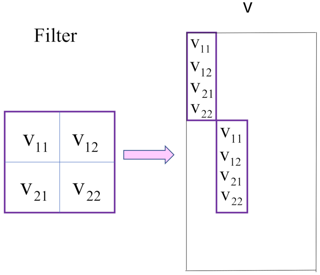
To express this operation with mathematical equations, we squash each submatrix that multiplies with the filter into a vector. More specifically, the red square of the input array in Figure 2 is squashed into the vector $(x_{11},x_{12},x_{21},x_{22})$. Then, we put all squashed vectors into a matrix X in order of the filter sliding, as shown in Figure 2. The filter is also squashed with a vector ${(v_{11},v_{12},v_{21},v_{22})}^T$ accordingly, and then is repeatedly put into the diagonal position of the matrix V, as shown in Figure 3. Other elements of V are 0. With X and V, the operation of the convolutional layer can be described with the matrix multiplication of X and V, as shown in Figure 4, i.e.,

$$\mathrm{Conv}=X·V$$

(10)

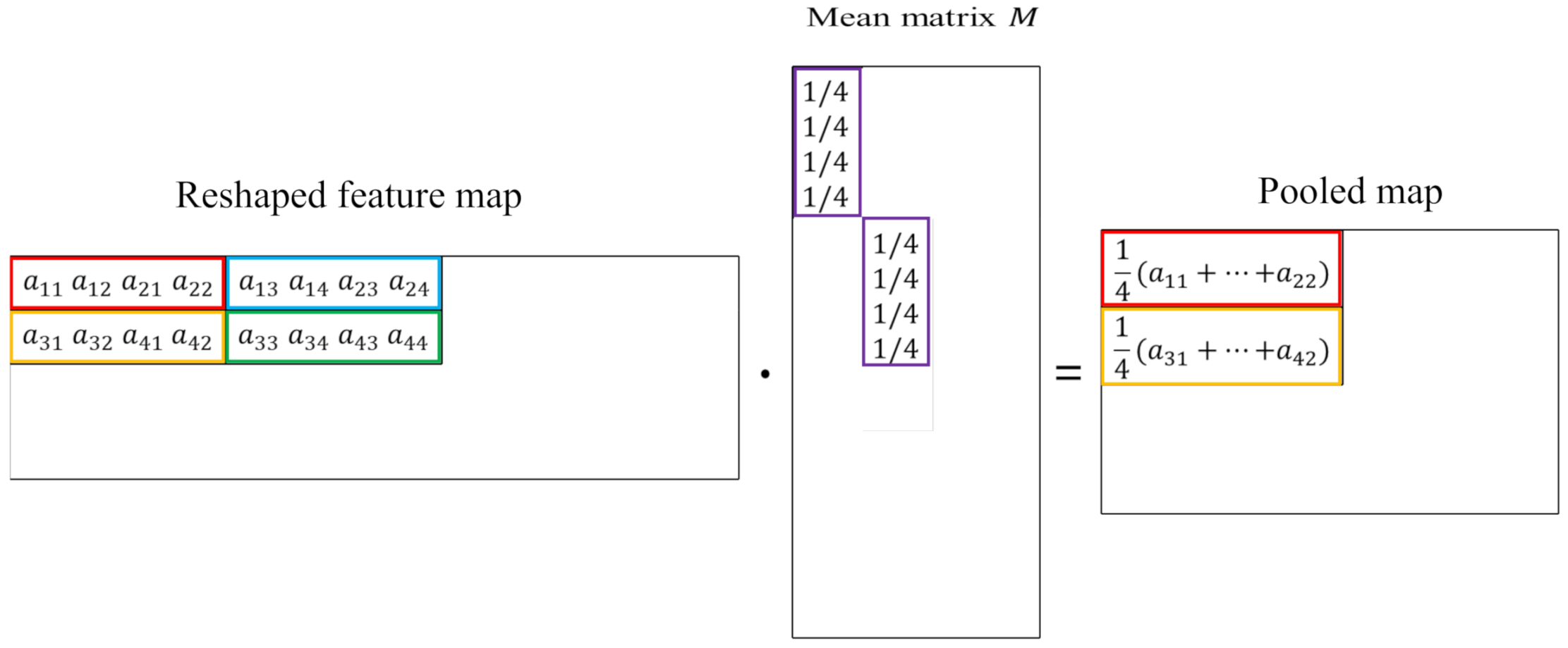
The mean pooling is assumed to be applied in $2\times 2$ patches of the feature map with a stride of $(2,2)$. It can also be expressed with the matrix multiplication, as shown in Figure 5. Each patch of the feature map is flattened into a vector and all the vectors are merged into a matrix as a reshaped feature map, as shown in Figure 5. The sliding mean window is flattened as a vector ${(\frac{1}{4},\frac{1}{4},\frac{1}{4},\frac{1}{4})}^T$ and is repeatedly put into the diagonal position of the mean matrix M, as shown in Figure 5. As in Equation (10), the mean pooling operation can be expressed with the matrix multiplication:

$$\mathrm{mean}\mathrm{pooling}=X·M.$$

(11)

Now, given an input array X, the processing procedure from the convolution to the output layer can be expressed by mathematical equations. The output of the convolution layer is

$$A=G\left(X\right)·V,$$

(12)

where the function G means the reshape operation shown in Figure 2. After the ReLU layer, the matrix $\mathrm{ReLU}\left(A\right)$ is reshaped as $G\left(\mathrm{ReLU}\right(A\left)\right)$. In the pooling layer, the mean function is used

$$\mathrm{mean}\mathrm{pooling}=G\left(\mathrm{ReLU}\right(A\left)\right)·M.$$

(13)

Then, the output matrix of the pooling layer is vectorized by column scan and this process is denoted by

$$S=F\left(\mathrm{mean}\mathrm{pooling}\right),$$

(14)

where the function F denotes the layer vectorized by the column. Finally, the fully connected layer is

$$O=g(U·S).$$

(15)

3.2. Convergence Results

To prove that our proposed method is feasible, here, we give the convergence results. For ease of understanding, we take the simplest single-layer CNN case as an example. This CNN includes one convolution, one pooling and one fully connected layer, where the convolution filter size is $(5,5)$ and the mean pooling size is $(2,2)$.

Given the training sample set ${\{X^j,T^j\}}_{j=1}^J$, each $X^j$ is assumed to be the $28\times 28$ input array and $T^j$ is the $10\times 1$ vector. According to Equations (12)–(15), the error function of Equation (8) can be expressed as

$$\begin{array}{cc}\hfill E& =\frac{1}{2J}\sum _{j=1}^J\sum _{i=1}^{10}{(o_i^j-t_i^j)}^2+\lambda \sum _{k=1}^{144}{\left(\sum _{i=1}^{10}f\left(u_{ik}\right)\right)}^{\frac{1}{2}}\hfill \\ \hfill & =\frac{1}{2J}\sum _{j=1}^J\sum _{i=1}^{10}{\left(g(U_i·F(G\left(\mathrm{ReLU}(G\left(X^j\right)·V)\right)·M))-t_i^j\right)}^2+\lambda \sum _{k=1}^{144}{\left(\sum _{i=1}^{10}f\left(u_{ik}\right)\right)}^{\frac{1}{2}}\hfill \\ \hfill & =\sum _{j=1}^J\sum _{i=1}^{10}{g}_{ji}(U_i·S)+\lambda \sum _{k=1}^{144}{\left(\sum _{i=1}^{10}f\left(u_{ik}\right)\right)}^{\frac{1}{2}},\hfill \end{array}$$

(16)

where $g_{ji}\left(t\right)=\frac{1}{2J}{(g\left(t\right)-t_i^j)}^2$, $U_i$ is the i-th row vector of U.

Training a CNN involves finding a suitable V and U so that E reaches the minimum [27]. For this reason, the gradient descent method [28] is adopted. Notice that the mean matrix M does not need to be trained. In the backpropagation algorithm, V and U are changed according to the gradient descent direction of E. The partial derivative of E with respect to the element $u_{ik}$ of U is as follows:

$$\begin{array}{cc}\hfill E_{u_{ik}}& =\sum _{j=1}^J{g}_{ji}^{\prime }(U_i·S)·S_k+\lambda \frac{f^{\prime }\left(u_{ik}\right)}{2\sqrt{{\displaystyle \sum _{i=1}^{10}}f\left(u_{ik}\right)}},(k=1,\cdots ,144).\hfill \end{array}$$

(17)

The partial derivative of E with respect to the element $v_{ij}$ of the convolution filter V is the same as the original CNN because the partial derivative of the penalty term in Equation (16) with respect to $v_{ij}$ is zero. That is,

$$\begin{array}{cc}\hfill E_{v_{pl}}& =\sum _{j=1}^J\sum _{i=1}^{10}{g}_{ji}^{\prime }(U_i·S)\sum _{k=1}^{144}{u}_{ik}\frac{\partial S_k}{\partial v_{pl}}\hfill \\ \hfill & =\sum _{j=1}^J\sum _{i=1}^{10}{g}_{ji}^{\prime }(U_i·S)\sum _{m=0}^{11}\sum _{h=1}^{12}{u}_{i,12m+h}\frac{\partial s_{m+1,h}}{\partial v_{pl}}\hfill \\ \hfill & =\frac{1}{4}\sum _{j=1}^J\sum _{i=1}^{10}{g}_{ji}^{\prime }(U_i·S)\sum _{m=0}^{11}\sum _{h=1}^{12}{u}_{i,12m+h}\hfill \\ \hfill & ·(\delta \left(a_{m+1,h}\right)\frac{\partial a_{m+1,h}}{\partial v_{pl}}+\delta \left(a_{m+1,h+1}\right)\frac{\partial a_{m+1,h+1}}{\partial v_{pl}}\hfill \\ \hfill & +\delta \left(a_{m+2,h}\right)\frac{\partial a_{m+2,h}}{\partial v_{pl}}+\delta \left(a_{m+2,h+1}\right)\frac{\partial a_{m+2,h+1}}{\partial v_{pl}})\hfill \\ \hfill & =\frac{1}{4}\sum _{j=1}^J\sum _{i=1}^{10}{g}_{ji}^{\prime }(U_i·S)\sum _{m=0}^{11}\sum _{h=1}^{12}{u}_{i,12m+h}\hfill \\ \hfill & ·(\delta \left(a_{m+1,h}\right)x_{m+p,h+l-1}+\delta \left(a_{m+1,h+1}\right)x_{m+p,h+l}\hfill \\ \hfill & +\delta \left(a_{m+2,h}\right)x_{m+p+1,h+l-1}+\delta \left(a_{m+2,h+2}\right)x_{m+p+1,h+l}),\hfill \end{array}$$

(18)

where $\delta$ is the derivative function of the rectified linear units function:

$$\delta \left(t\right)=\left\{\begin{array}{c}1,t>0,\hfill \\ 0,t\le 0.\hfill \end{array}\right.$$

Thus far, we have given the step direction of U and V by (17) and (18), respectively. Now, we proceed to give the step direction of the biases. The partial derivative of the biases can be computed similarly as shown in [29]; the reader can refer to this article for more details.

We combine all weights and biases into a large vector W. Then, the parameter updating algorithm of $SG{L}_{1/2}$ is defined as follows:

$$W^{n+1}=W^n+▵W^n=W^n-\eta E_{W^n},$$

(19)

where $\eta$ is the learning rate and n is the iteration step.

The convergence proof needs some Assumptions as follows:

(1)

$\left|\right|W^n\left|\right|$$(n=0,1,2,\dots )$ are uniformly bounded, where $W^n$ is the error of the n-th step.

(2)

$\lambda$ and $\eta$ are chosen to satisfy $\eta \le min\{\frac{1}{C_6},\frac{1}{C_5+\lambda C_7}\}$, where $C_5$, $C_6$ and $C_7$ are constants defined below.

(3)

There exists a compact set $\Phi$ such that $W^n\in \Phi$ and ${\Phi }_0=\{W\in \Phi :E_W=0\}$ contains finite points.

Theorem 1.

Let the error function be Equation (8) and the weight sequence $\left\{W^n\right\}$ be generated by Equation (19) with any initial value $W^0$. If Assumptions (1)–(2) are available, then

(i) 

$E\left(W^n\right)\ge E\left(W^{n+1}\right),n=0,1,2,\dots ;$

(ii) 

There exists $E^{\ast }\ge 0$, such that $\underset{n\to \infty }{lim}E\left(W^n\right)=E^{\ast }$;

(iii) 

The weak convergence holds, i.e., $\underset{n\to \infty }{lim}\left|\right|E_{W^n}{\left|\right|}_2=0$.

In addition, if the assumption (3) also holds, then the strong convergence result holds:

(iv) 

There exists a point $W^{\ast }\in {\Phi }_0$ such that $\underset{n\to \infty }{lim}{W}^n=W^{\ast }$.

The proof process is not the focus of this article, so we include it in the Appendix A.

4. Numerical Experiments and Discussion

We evaluate $SG{L}_{1/2}$ in different ways, such as nodes [30] and weights sparsity [31], training and testing accuracy, the norm of weight gradient and the convergence speed, on four typical benchmark datasets: Mnist [32], Letter Recognition [33], Cifar 10 [34] and Crowded Mapping. For parameter sparsity, $SG{L}_{1/2}$ is compared with some conventional and sparse algorithms including $G{L}_1$, $G{L}_2$ and $G{L}_{1/2}$. Moreover, we investigate the test accuracy by comparing $SG{L}_{1/2}$ with the above regularization algorithms.

For the following numerical experiments, we refer to the arithmetic optimization algorithm [35] and adopt a five-fold cross-validation technique [36,37,38]. We randomly divide the dataset into five parts, where the sample size is equal (or almost equal). The network learning of these four algorithms is carried out five times. Each time, one of the five parts is selected in turn as the test sample set, and the other four parts are used as the training sample sets. Then, we rearrange the five-part samples and start the process again. This process is repeated twenty times. The experiment process is given in Algorithm 1.

Algorithm 1 The experiment process.

Step 1: Input the data and calculate the corresponding actual output; Step 2: Calculate the difference between the actual output and the ideal output; Step 3: Give the error function according to these four algorithms; Step 4: Update the weights of the fully connected layer according to the error function of step 3; Step 5: Keep iterating, repeat steps 2–4; Step 6: Calculate the pruned nodes, pruned weights of surviving weights and classification accuracies under these four methods, respectively; Step 7: Contrast.

Finally, for each dataset and algorithm, we obtain one hundred classification results. Each result contains the rate of pruned nodes (Rate of PN) (cf. Equation (20)), the rate of pruned weights of the remaining nodes (Rate of PW) (cf. Equation (21)), training accuracy (Training Acc.) and test accuracy (Test Acc.). The averages of these numerical results are listed in

Table 1. Mnist: Comparison of Rate of PN, Rate of PW, Training Acc. and Test Acc. by using $G{L}_1$, $G{L}_2$, $G{L}_{1/2}$ and $SG{L}_{1/2}$ learning algorithms.

Algorithm	Rate of PN (%)	Rate of PW (%)	Training Acc. (%)	Test Acc. (%)
$G{L}_1$	15.50	2.60	99.75	99.13
$G{L}_2$	16.17	3.16	99.80	99.15
$G{L}_{1/2}$	12.33	19.83	99.67	99.06
$SG{L}_{1/2}$	19.33	17.79	99.83	99.24

,

Table 2. Letter: Comparison of Rate of PN, Rate of PW, Training Acc. and Test Acc. by using $G{L}_1$, $G{L}_2$, $G{L}_{1/2}$ and $SG{L}_{1/2}$ learning algorithms.

Algorithm	Rate of PN (%)	Rate of PW (%)	Training Acc. (%)	Test Acc. (%)
$G{L}_1$	7.78	1.95	89.75	87.42
$G{L}_2$	8.89	2.86	89.81	87.60
$G{L}_{1/2}$	5.56	18.37	89.67	86.83
$SG{L}_{1/2}$	15.56	12.04	90.43	87.93

,

Table 3. Cifar 10: Comparison of Rate of PN, Rate of PW, Training Acc. and Test Acc. by using $G{L}_1$, $G{L}_2$, $G{L}_{1/2}$ and $SG{L}_{1/2}$ learning algorithms.

Algorithm	Rate of PN (%)	Rate of PW (%)	Training Acc. (%)	Test Acc. (%)
$G{L}_1$	12.7	2.20	87.95	82.84
$G{L}_2$	13.4	2.63	88.07	83.26
$G{L}_{1/2}$	9.02	18.05	87.36	82.30
$SG{L}_{1/2}$	20.61	17.27	88.39	83.86

and

Table 4. Crowded Mapping: Comparison of Rate of PN, Rate of PW, Training Acc. and Test Acc. by using $G{L}_1$, $G{L}_2$, $G{L}_{1/2}$ and $SG{L}_{1/2}$ learning algorithms.

Algorithm	Rate of PN (%)	Rate of PW (%)	Training Acc. (%)	Test Acc. (%)
$G{L}_1$	11.46	1.85	93.58	92.76
$G{L}_2$	12.85	3.07	94.39	93.58
$G{L}_{1/2}$	8.93	19.65	92.54	91.90
$SG{L}_{1/2}$	22.60	17.28	95.21	94.63

for these four datasets.

$$\mathrm{Rate}\mathrm{of}\mathrm{PN}=\frac{\mathrm{Pruned}\mathrm{nodes}}{\mathrm{All}\mathrm{nodes}},$$

(20)

$$\mathrm{Rate}\mathrm{of}\mathrm{PW}=\frac{\mathrm{Pruned}\mathrm{weights}\mathrm{of}\mathrm{surviving}\mathrm{nodes}}{\mathrm{Surviving}\mathrm{nodes}\times \mathrm{Output}\mathrm{nodes}}.$$

(21)

For an output node, the ideal output value is 1 or 0. When we evaluate the error between the ideal and real output values, we use the following “40-20-40” standard [39]: The actual output values of the output nodes between $0.00$ and $0.40$ are regarded as 0, values between $0.60$ and $1.00$ are regraded as 1, and values between $0.40$ and $0.60$ are regraded as uncertain and are considered incorrect.

4.1. Mnist Problem

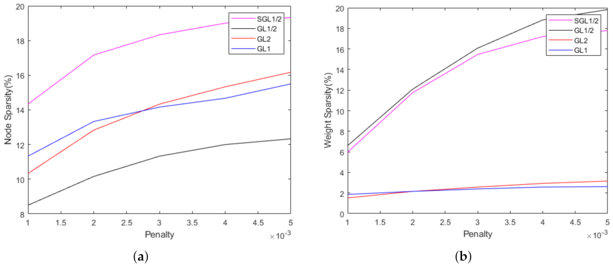
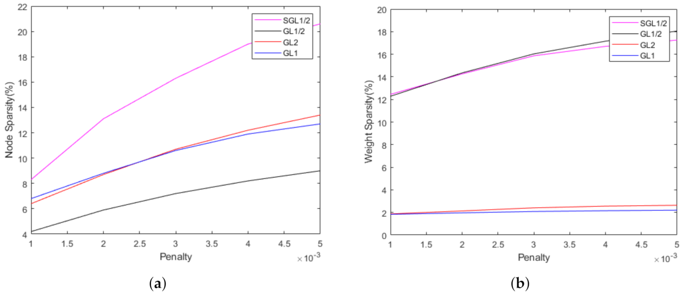
MNIST is a dataset for the study of handwritten numeral recognition, which contains 70,000 examples of $28\times 28$ pixel images of the digits 0–9. For these four algorithms, we set the learning rate $\eta =0.03$. The maximum iteration training step is 1000. In order to show the sparsity, we give the node sparsity and weight sparsity performances for $\lambda =0.001,0.002,0.003,0.004,0.005$ of these four algorithms (see Figure 6; y-axis represents the percentage of the number of pruned nodes and pruned weights of the remaining nodes, respectively). The sparsity will become worse when $\lambda >0.005$. Therefore, we choose $\lambda =0.005$ to compare these algorithms. The performances of these four group lasso algorithms are compared in Table 1. We can see that, in terms of the sparsity, the performance of $SG{L}_{1/2}$ is better than $G{L}_2$, $G{L}_1$ and $G{L}_{1/2}$. In terms of of accuracy, $SG{L}_{1/2}$ is also the best. 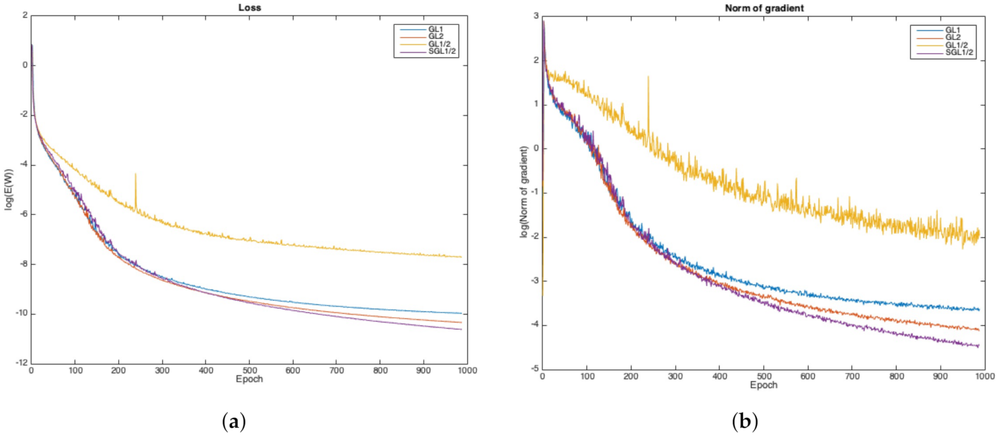Figure 7a presents the loss functions of these four group lasso algorithms. Obviously, we can see that the $SG{L}_{1/2}$ approach has the lowest error after training, and $SG{L}_{1/2}$ has a large fluctuation during the training process.

We show the gradient norms of $G{L}_1$, $G{L}_2$, $G{L}_{1/2}$ and $SG{L}_{1/2}$ in Figure 7b, where the oscillation [40,41] of $G{L}_{1/2}$ is presented. From Figure 7, we find that the $SG{L}_{1/2}$ regularizer eliminates the oscillation and guarantees the convergence, as predicted in Theorem 1.

4.2. Letter Recognition Problem

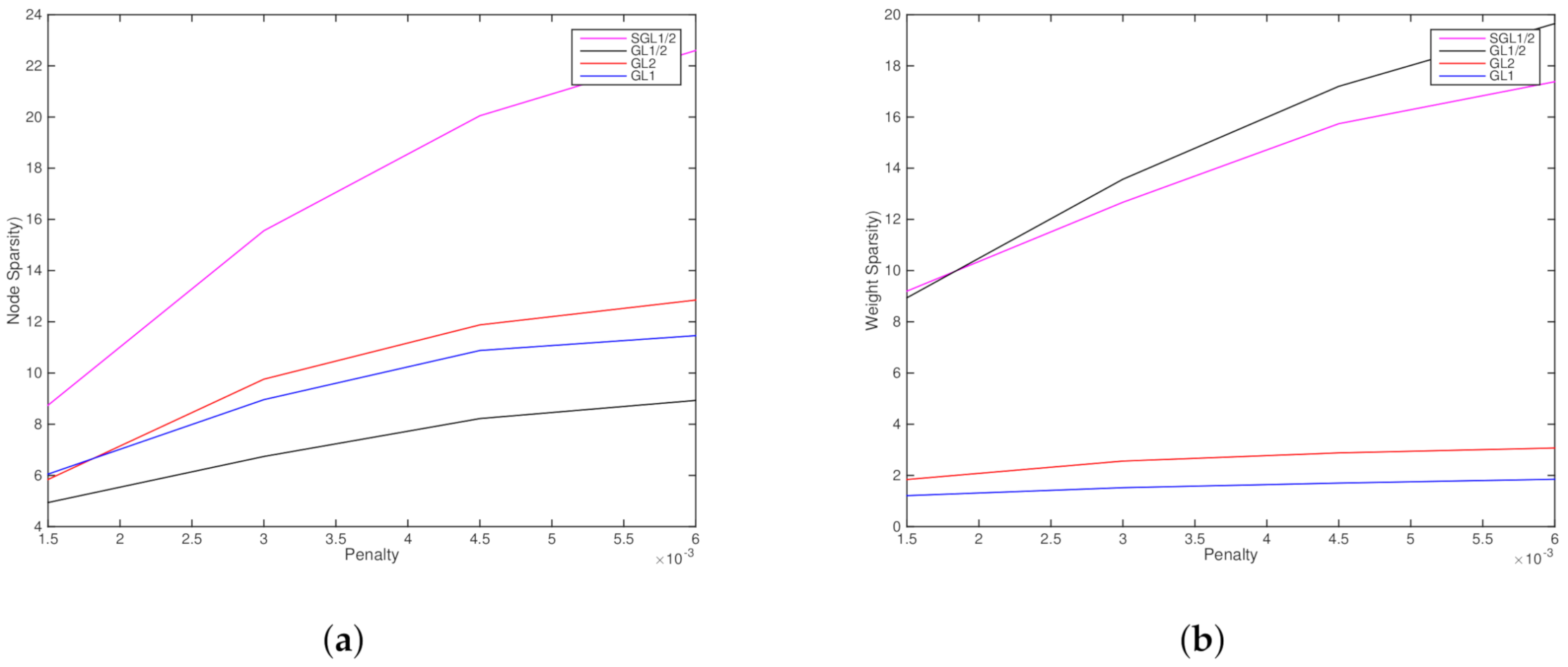
The Letter Recognition dataset consists of 20,000 samples with 16 attributes. Each 16-dimensional instance within this database represents a capital typewritten letter in one of twenty fonts. For these four algorithms, we set the learning rate $\eta =0.05$. The maximum iteration training step is 1000. In order to show the sparsity, we give the node sparsity and weight sparsity performances for $\lambda =0.002,0.004,0.006,0.008$ of these four algorithms (see Figure 8). The sparsity will become worse when $\lambda >0.008$. Therefore, we choose $\lambda =0.008$ to compare these algorithms. The performances of $G{L}_2$, $G{L}_1$, $G{L}_{1/2}$ and $SG{L}_{1/2}$ are compared in Table 2. We see that, in terms of sparsity, the performance of $SG{L}_{1/2}$ is better than $G{L}_2$, $G{L}_1$ and $G{L}_{1/2}$. In terms of accuracy, $SG{L}_{1/2}$ is also the best among the above-mentioned four algorithms. Figure 9a presents the loss functions of these four group lasso algorithms. Obviously, we can see that the $SG{L}_{1/2}$ approach has the lowest error after training, and $SG{L}_{1/2}$ has a large fluctuation during the training process.

We show the gradient norms of $G{L}_1$, $G{L}_2$, $G{L}_{1/2}$ and $SG{L}_{1/2}$ in Figure 9b, where the oscillation of $G{L}_{1/2}$ is presented. From Figure 9, we find that the $SG{L}_{1/2}$ regularizer eliminates the oscillation and guarantees the convergence, as predicted in Theorem 1.

4.3. Cifar 10 Problem

The Cifar 10 dataset consists of 60,000 images, each of which is a $32\times 32$ color map. This dataset contains 10 classes (airplane, automobile, bird, cat, deer, dog, frog, horse, ship and truck), with 6000 images per class. There are 50,000 training images and 10,000 test images. For these four algorithms, we set the learning rate $\eta =0.03$. The maximum iteration training step is 1000. In order to show the sparsity, we give the node sparsity and weight sparsity performances for $\lambda =0.001,0.002,0.003,0.004,0.005$ of these four algorithms (see Figure 10). The sparsity will become worse when $\lambda >0.005$. Therefore, we choose $\lambda =0.005$ to compare these algorithms. The performances of these four group lasso algorithms are compared in Table 3. We see that, in terms of of sparsity, the performance of $SG{L}_{1/2}$ is better than $G{L}_2$, $G{L}_1$ and $G{L}_{1/2}$. In terms of accuracy, $SG{L}_{1/2}$ is also the best. Figure 11a presents the loss functions of these four group lasso algorithms. Obviously, we can see that the $SG{L}_{1/2}$ approach has the lowest error after training, and $SG{L}_{1/2}$ has a large fluctuation during the training process.

We show the gradient norms of $G{L}_1$, $G{L}_2$, $G{L}_{1/2}$ and $SG{L}_{1/2}$ in Figure 11b, where the oscillation of $G{L}_{1/2}$ is presented. From Figure 11, we find that the $SG{L}_{1/2}$ regularizer eliminates the oscillation and guarantees the convergence, as predicted in Theorem 1.

4.4. Crowded Mapping

The Crowded Mapping dataset consists of 10,546 samples with 28 attributes, and these samples are divided into six classes. For these four algorithms, we set the learning rate $\eta =0.05$. The maximum iteration training step is 1000. In order to show the sparsity, we give the node sparsity and weight sparsity performances for $\lambda =0.0015,0.003,0.045,0.006$ of these four algorithms (see Figure 12). The sparsity will become worse when $\lambda >0.006$. Therefore, we choose $\lambda =0.006$ to compare these four algorithms. The performances of the $G{L}_1$, $G{L}_2$, $G{L}_{1/2}$ and $SG{L}_{1/2}$ methods are compared in Table 4. We see that, in terms of sparsity, the performance of $SG{L}_{1/2}$ is better than $G{L}_2$, $G{L}_1$ and $G{L}_{1/2}$. In terms of accuracy, $SG{L}_{1/2}$ is also the best among the above-mentioned four algorithms. Figure 13a presents the loss functions of these four group lasso algorithms. Obviously, we can see that the $SG{L}_{1/2}$ algorithm has the lowest error after training, and $SG{L}_{1/2}$ has a large fluctuation during the training process.

We show the gradient norms of $G{L}_1$, $G{L}_2$, $G{L}_{1/2}$ and $SG{L}_{1/2}$ in Figure 13b, where the oscillation of $G{L}_{1/2}$ is presented. From Figure 13, we find that the $SG{L}_{1/2}$ regularizer eliminates the oscillation and guarantees the convergence, as predicted in Theorem 1.

From the above experiments on the four datasets, it is easy to see that the $G{L}_1$ and $G{L}_2$ algorithms have better sparsity at the node level, and the $G{L}_{1/2}$ algorithm has better sparsity at the weight level. In some applications, the sparsity at the weight level is also of great significance. If the sparseness of the integrated node and weight level is better, the number of weights that need to be calculated and updated will be reduced in the process of training the CNNs. Furthermore, it also leads to a reduction in the amount of calculation and saves storage space. Compared with the $G{L}_1$ and $G{L}_2$ algorithms, the $SG{L}_{1/2}$ algorithm has better sparsity at the node level and the weight level, and can also improve the classification performance. Compared with the $G{L}_{1/2}$ algorithm, the theoretical analysis and numerical experiment are carried out to verify that the $SG{L}_{1/2}$ algorithm improves the sparsity at the node level, and at the same time improves the classification performance.

4.5. Discussion

Table 1, Table 2, Table 3 and Table 4, respectively, show the performance comparison of PN, PW, training accuracies and test accuracies under these four methods. In terms of the sparsity, the PN calculation results of the $SG{L}_{1/2}$ method are much better than the other three methods, especially the $G{L}_{1/2}$ method. As for the PW, although the surviving node of the $G{L}_{1/2}$ has a higher rate of pruned weights of surviving weights, the rate of pruned nodes is too low, such that the sparsity of the $G{L}_{1/2}$ method is still far lower than that of the $SG{L}_{1/2}$ method. In terms of classification accuracy, the $SG{L}_{1/2}$ method is slightly higher than other methods, which means that this method can improve the sparsity without damaging the classification accuracy.

We can find that the specificity of CNNs is not actually used in the experiments, so the $SG{L}_{1/2}$ method can be widely applied to other neural network models.

5. Conclusions

Our main task was to introduce the $SG{L}_{1/2}$ algorithm. Based on the $G{L}_1$ and $G{L}_2$ algorithms, replacing 1-norm and 2-norm with $\frac{1}{2}$-norm can greatly improve the sparsity of the network weight level, but it does not help to achieve better sparsity of the node level. The non-smooth penalty term at the origin is the root cause of the poor sparsity of the $G{L}_{1/2}$ algorithm at the node level.

To this end, in this paper, a smooth group $L_{1/2}$ ($SG{L}_{1/2}$) regularization term is introduced into the batch gradient learning algorithm to prune the CNN. The feasibility analysis of the $SG{L}_{1/2}$ method for the fully connected layer of the CNN is performed. Numerical experiments show that the sparsity and convergence of $SG{L}_{1/2}$ give better results in terms of both the rate of pruned hidden nodes and weights of the remaining hidden nodes compared to $G{L}_{1/2}$, $G{L}_1$ and $G{L}_2$. In addition, the $SG{L}_{1/2}$ regularizer not only overcomes the oscillation phenomenon during the training process, but also achieves better classification performance.

In fact, the $SG{L}_{1/2}$ regularization algorithm provides a strategy to improve the sparsity of hidden layers of neural networks, not only for CNNs. Therefore, the performance of the $SG{L}_{1/2}$ regularization algorithm on other neural network models is also worthy of further verification. However, the $SG{L}_{1/2}$ algorithm is not particularly obvious in improving the classification accuracy. In future work, we will focus on continuing to improve the $SG{L}_{1/2}$ algorithm to achieve better classification performance of the neural network.