Direct Determination of Reduced Models of a Class of Singularly Perturbed Nonlinear Systems on Three Time Scales in a Bond Graph Approach

Abstract

One of the most important features in the analysis of the singular perturbation methods is the reduction of models. Likewise, the bond graph methodology in dynamic system modeling has been widely used. In this paper, the bond graph modeling of nonlinear systems with singular perturbations is presented. The class of nonlinear systems is the product of state variables on three time scales (fast, medium, and slow). Through this paper, the symmetry of mathematical modeling and graphical modeling can be established. A main characteristic of the bond graph is the application of causality to its elements. When an integral causality is assigned to the storage elements that determine the state variables, the dynamic model is obtained. If the storage elements of the fast dynamics have a derivative causality and the storage elements of the medium and slow dynamics an integral causality is assigned, a reduced model is obtained, which consists of a dynamic model for the medium and slow time scales and a stationary model of the fast time scale. By applying derivative causality to the storage elements of the fast and medium dynamics and an integral causality to the storage elements of the slow dynamics, the quasi-steady-state model for the slow dynamics is obtained and stationary models for the fast and medium dynamics are defined. The exact and reduced models of singularly perturbed systems can be interpreted as another symmetry in the development of this paper. Finally, the proposed methodology was applied to a system with three time scales in a bond graph approach, and simulation results are shown in order to indicate the effectiveness of the proposed methodology.

1. Introduction

The modeling, analysis, and control of high-order systems are an interesting challenge to give adequate results. Furthermore, some of these systems may present different time scales, which are called singularly perturbed systems. Systems of two time scales are the most common determining slow and fast variables. These systems are characterized by having parasitic parameters.

Essential references of systems with singular perturbations are found in [1,2]. Modeling and its properties of nonlinear systems with multiple time scales are proposed in [3]. The correct application of some of the singular perturbation methods derived in the reduction of systems given the exact decomposition of the slow and fast modes was proposed in [4]. Systems with singular perturbations indicate the presence of the parasitic parameter, and the control of this parameter was described in [5]. Exponential stability applied to nonlinear singularly perturbed systems was analyzed in [6]. The asymptotic stability of time-varying systems with singular perturbations was introduced in [7]. Observers of singularly perturbed systems were applied in [8,9]. The robust stability of systems with singular perturbations was described in [10].

More recent references and three time scales are cited below. The control of a helicopter system that determines a system with three time scales was presented in [11]. Furthermore, sliding mode control for systems with three time scales and disturbances was proposed in [12]. An adaptive fault-tolerant control for LTI systems with two or three time scale was presented in [13]. The control theory with applications in the period 1984–2001 for systems with singular perturbations was described in [14].

The bond graph methodology allows modeling, analyzing, and controlling systems in different energy domains (electrical, mechanical, hydraulic, thermal, magnetic) [15,16]. Some papers have been published on systems with singular perturbations with bond graphs within which the following can be cited. The models and their simplification to singular perturbation methods were described in [17]. Reciprocal systems to obtain fast dynamics were introduced in [18]. Reduced models of LTI systems with singular perturbations on two time scales with different causalities were proposed in [19]. The determination of approximate models of LTI systems with mixed causalities to the storage elements in the bond graph was presented in [20].

The determination of bond graph models and their realization in the state space indicate the graphical and mathematical symmetry of these systems.

The different dynamics of a system through causal loops were identified in [18,21]. State feedback using an observer for LTI systems in the physical domain was proposed in [22]. Furthermore, the modeling of a class of nonlinear systems with two time scales was presented in [23]. LTI systems with three time scales, their modeling, and their reduction with mixed causalities in bond graphs were introduced in [24].

Currently, there are some software programs available for modeling and system analysis in a bond graph approach, for example the 20-sim software developed at the university of Twente, BONDLAB introduced by Bond Lab Technologies, SYMBOLS 2000 presented by Mukherjee and Samantaray, and CAMPG developed by Cadsim Engineering.

Control systems modeled in bond graphs require the design of the control law existing in different procedures, for example bond-graph-based control by Gawthrop [25,26] and bond graphs in control by Karnopp [27]. A slow state estimated feedback applied to a bond graph model of a singularly perturbed system was proposed in [22]. Furthermore, a composite feedback control of a system with singular perturbations in the physical domain was presented in [28].

In this paper, bond graph models of a class of nonlinear systems with singular perturbations on three time scales (fast, medium, slow) are proposed. These systems can have linearly independent and dependent state variables on each time scale. Due to the properties of singularly perturbed systems, reduced models can be obtained. The deduction and comparison of reduced models from the exact models can be manifested as a symmetry of the systems with singular perturbations.

The first reduced model is when the fast dynamics have converged, which is applied to the storage elements that represent these dynamics as a derivative causality. The next reduced model is obtained by assigning derivative causality to the elements of the medium dynamics, indicating that these dynamics have converged. Therefore, the traditional quasi-steady-state model with slow dynamics in a bond graph approach is determined. This paper is based on [19,23]. However, the extension to three time scales to a class of nonlinear systems and the different dynamics can be linearly independent and dependent, offering the originality of this paper.

Bond graph modeling has been used extensively in robotic systems and is applied to internal combustion and electric vehicles today [29]. Furthermore, thermal and chemical systems have been modeled with bond graphs [15]. These systems generally determine nonlinear models on various time scales, so this paper can be useful to analyze the behavior of reduced models. Complex dynamic systems are an interesting challenge to model in bond graphs

This paper is organized as follows: Section 2 gives the analysis of systems with singular perturbations in the algebraic approach. The modeling and reduction in the bond graph of systems with three time scales is presented in Section 3. A case of study of an electromechanical system by obtaining the reduced models in the physical domain is described in Section 4. Finally, in Section 5, the conclusions are given.

2. Singular Perturbation Method

A singularly perturbed nonlinear system is expressed by:

$$\begin{array}{ccc}\hfill {\stackrel{•}{x}}_1& =& f\left(x_1,x_2,u,\epsilon ,t\right),x_1\left(t=0\right)=x_1\left(0\right)x_1\in {\Re }^n\hfill \end{array}$$

(1)

$$\begin{array}{ccc}\hfill \epsilon {\stackrel{•}{x}}_2& =& g\left(x_1,x_2,u,\epsilon ,t\right),x_2\left(t=0\right)=x_2\left(0\right)x_2\in {\Re }^m\hfill \end{array}$$

(2)

It is assumed that in the domain of interest, f and g are continuous differentiable functions of their arguments $x_1$, $x_2$, u, $\epsilon$, and t. Due to the characteristics of systems with singular perturbations whose complete order is $\left(n+m\right)$ containing small time constants, it is possible to neglect them by setting $\epsilon =0$ in (2):

$$0=g\left(\overline{x_1},\overline{x_2},\overline{u},0,t\right)$$

(3)

and substituting (3) into (1):

$$\stackrel{•}{\overline{x_1}}=f\left(\overline{x_1},\overline{x_2},\overline{u},0,t\right)$$

(4)

determines a reduced differential equation of order n and an algebraic equation of order m.

It is assumed that one of the several solutions of (3) is defined by:

$$\overline{x_2}=\varphi \left(\overline{x_1},\overline{u},t\right)$$

(5)

and substituting (5) into (4), the quasi-steady-state model is obtained by:

$$\begin{array}{ccc}\hfill \stackrel{•}{\overline{x_1}}& =& f\left(\overline{x_1},\varphi \left(\overline{x_1},\overline{u},t\right),\overline{u},t\right)\hfill \\ & =& \overline{f}\left(\overline{x_1},\overline{u},t\right)\hfill \end{array}$$

(6)

The validity of the given reduction of a system with singular perturbations is due to the Tikhonov theorem, which requires the following assumptions.

Assumption 1

([1,2]). The functions f and g are continuous with the variables x, y, and t.

Assumption 2

([1,2]). The differential equation of fast dynamics on the fast time scale:

$$\frac{d{x}_2\left(\tau \right)}{d\tau }=g\left[\overline{x_1},x_2\left(\tau \right),\overline{u},0,t\right]$$

(7)

where $\overline{x_1}$ and t are fixed parameters, is called the boundary layer equation of the system (1) and (2).

Assumption 3

([1,2]). The root $\overline{x_2}=\varphi \left(\overline{x_1},\overline{u},t\right)$ of the equation $g\left(\overline{x_1},\overline{x_2},\overline{u},0,t\right)=0$ is called an isolated root in a domain D of the set of variables $x_1$, u, and t, if there exists an $\epsilon >0$ such that the equation $g\left(\overline{x_1},\overline{x_2},\overline{u},0,t\right)=0$ has no solution other than $\varphi \left(\overline{x_1},\overline{u},t\right)$ for $\left|\overline{x_2}-\varphi \left(\overline{x_1},\overline{u},t\right)\right|<\epsilon$.

Assumption 4

([1,2]). The isolated root $\overline{x_2}=\varphi \left(\overline{x_1},\overline{u},t\right)$ is called stable in D if, for all points $\left(x_1,u,t\right)\in D$, the points $\overline{x_2}=\varphi \left(\overline{x_1},\overline{u},t\right)$ are asymptotically stable equilibrium points according to Lyapunov with Equation (7) as $\tau \to \infty$. This means that the Jacobian matrix $g_{x_2}$ has all eigenvalues with negative real parts,

$$\mathit{Re}\lambda \left\{\frac{\partial g}{\partial x_2}\right\}\le -c<0$$

(8)

Assumption 5

([1,2]). The region of influence R of an isolated stable root $\overline{x_2}=\varphi \left(\overline{x_1},\overline{u},t\right)$ is the set of points $\left[x_1\left(0\right),x_2\left(0\right),u\left(0\right),t_0\right]$ such that the solution of (7) satisfying the initial condition $x_2\left(\tau =0\right)=x_2\left(0\right)$ tends to the value $\varphi \left(\overline{x_1}\left(0\right),\overline{u}\left(0\right),t_0\right)$, as $\tau \to \infty$.

With the established assumptions, the Tikhonov theorem is enunciated.

Theorem 1

([1,2]). Let Assumptions 1 to 5 be satisfied. Then, the solutions $x_1\left(t,\epsilon \right)$ and $x_2\left(t,\epsilon \right)$ of the full system (1) and (2) are related to the solutions $\overline{x_1}$ and $\overline{x_2}$ of the degenerate model (3) and (4) as:

$$\begin{array}{ccc}\hfill \underset{\epsilon \to 0}{lim}\left[x_1\left(t,\epsilon \right)\right]& =& \overline{x_1}\left(t\right),0\le t\le T\hfill \end{array}$$

(9)

$$\begin{array}{ccc}\hfill \underset{\epsilon \to 0}{lim}\left[x_2\left(t,\epsilon \right)\right]& =& \overline{x_2}\left(t\right),0<t\le T\hfill \end{array}$$

(10)

where T is any value such that $\overline{x_2}=\varphi \left(\overline{x_1},\overline{u},t\right)$ is an isolated stable root of $g\left(\overline{x_1},\overline{x_2},\overline{u},0,t\right)=0$ for $0\le t\le T$. Thus, the convergence is uniform in $0\le t\le T$ for $x_1\left(t,\epsilon \right)$ and in any interval $0<t_1\le t\le T$ for $x_2\left(t,\epsilon \right)$.

A singular perturbed system with three time scales is defined by:

$$\begin{array}{ccc}\hfill {\stackrel{•}{x}}_1& =& f\left(x_1,x_2,x_3,u,{\epsilon }_1,{\epsilon }_2,t\right),x_1\left(t=0\right)=x_1\left(0\right)x_1\in {\Re }^n\hfill \end{array}$$

(11)

$$\begin{array}{ccc}\hfill {\stackrel{•}{x}}_2& =& g\left(x_1,x_2,x_3,u,{\epsilon }_1,{\epsilon }_2,t\right),x_2\left(t=0\right)=x_2\left(0\right)x_2\in {\Re }^m\hfill \end{array}$$

(12)

$$\begin{array}{ccc}\hfill {\stackrel{•}{x}}_3& =& h\left(x_1,x_2,x_3,u,{\epsilon }_1,{\epsilon }_2,t\right),x_3\left(t=0\right)=x_3\left(0\right)x_3\in {\Re }^l\hfill \end{array}$$

(13)

where f, g, and h are assumed to be sufficiently many times continuously differentiable functions for their arguments $x_1$, $x_2$, $x_3$, ${\epsilon }_1$, and ${\epsilon }_2$.

In this paper, the product of state variables is the specific class of nonlinear systems modeled and analyzed. These systems are described by:

$$\left[\begin{array}{c}{\stackrel{•}{x}}_1\left(t\right)\\ {\epsilon }_1{\stackrel{•}{x}}_2\left(t\right)\\ {\epsilon }_2{\stackrel{•}{x}}_3\left(t\right)\end{array}\right]=\left[\begin{array}{ccc}{A}_{11}\left(x\right)& A_{12}\left(x\right)& A_{13}\left(x\right)\\ A_{21}\left(x\right)& A_{22}\left(x\right)& A_{23}\left(x\right)\\ A_{31}\left(x\right)& A_{32}\left(x\right)& A_{33}\left(x\right)\end{array}\right]\left[\begin{array}{c}{x}_1\left(t\right)\\ x_2\left(t\right)\\ x_3\left(t\right)\end{array}\right]+\left[\begin{array}{c}{B}_1\left(x\right)\\ B_2\left(x\right)\\ B_3\left(x\right)\end{array}\right]u\left(t\right)$$

(14)

where the slow, medium, and fast dynamics are $x_1\left(t\right){\Re }^n$, $x_2\left(t\right){\Re }^m$, and $x_3\left(t\right){\Re }^l$, respectively, and the inputs are $u\left(t\right){\Re }^p$.

The first reduction of this system is obtained by neglecting the fast dynamics $\left({\epsilon }_2=0\right)$ deriving the following expressions:

$$\left[\begin{array}{c}\stackrel{•}{\overline{x_1}}\left(t\right)\\ {\epsilon }_1\stackrel{•}{\overline{x_2}}\left(t\right)\\ {\overline{x}}_3\left(t\right)\end{array}\right]=\overline{A}\left(x\right)\left[\begin{array}{c}\overline{x_1}\left(t\right)\\ \overline{x_2}\left(t\right)\end{array}\right]+\overline{B}\left(x\right)u\left(t\right)$$

(15)

where:

$$\begin{array}{ccc}\hfill \overline{A}\left(x\right)& =& \left[\begin{array}{cc}\overline{A_{11}}\left(x\right)& \overline{A_{12}}\left(x\right)\\ \overline{A_{21}}\left(x\right)& \overline{A_{22}}\left(x\right)\\ \overline{A_{31}}\left(x\right)& \overline{A_{32}}\left(x\right)\end{array}\right]\hfill \\ & =& \left[\begin{array}{cc}{A}_{11}\left(x\right)-A_{13}\left(x\right)A_{33}^{-1}\left(x\right)A_{31}\left(x\right)& A_{11}\left(x\right)-A_{13}\left(x\right)A_{33}^{-1}\left(x\right)A_{32}\left(x\right)\\ A_{21}\left(x\right)-A_{23}\left(x\right)A_{33}^{-1}\left(x\right)A_{31}\left(x\right)& A_{22}\left(x\right)-A_{23}\left(x\right)A_{33}^{-1}\left(x\right)A_{32}\left(x\right)\\ -A_{33}^{-1}\left(x\right)A_{31}\left(x\right)& -A_{33}^{-1}\left(x\right)A_{32}\left(x\right)\end{array}\right]\hfill \end{array}$$

(16)

and:

$$\overline{B}\left(x\right)=\left[\begin{array}{c}\overline{B_1}\left(x\right)\\ \overline{B_2}\left(x\right)\\ \overline{B_3}\left(x\right)\end{array}\right]=\left[\begin{array}{c}{B}_1\left(x\right)-A_{13}\left(x\right)A_{33}^{-1}\left(x\right)B_3\left(x\right)\\ B_2\left(x\right)-A_{23}\left(x\right)A_{33}^{-1}\left(x\right)B_3\left(x\right)\\ -A_{33}^{-1}\left(x\right)B_3\left(x\right)\end{array}\right]$$

(17)

The last reduction is achieved by removing the medium dynamics with ${\epsilon }_1=0$, and the system is described by:

$$\left[\begin{array}{c}\stackrel{•}{\widetilde{x_1}}\left(t\right)\\ \widetilde{x_2}\left(t\right)\end{array}\right]=\tilde{A}\left(x\right)\widetilde{x_1}\left(t\right)+\tilde{B}\left(x\right)u\left(t\right)$$

(18)

where:

$$\tilde{A}\left(x\right)=\left[\begin{array}{c}\widetilde{A_{11}}\\ \widetilde{A_{21}}\end{array}\right]=\left[\begin{array}{c}\overline{A_{11}}\left(x\right)-\overline{A_{12}}\left(x\right){\left[\overline{A_{22}}\left(x\right)\right]}^{-1}\overline{A_{21}}\left(x\right)\\ -{\left[\overline{A_{22}}\left(x\right)\right]}^{-1}\overline{A_{21}}\left(x\right)\end{array}\right]$$

(19)

and:

$$\tilde{B}\left(x\right)=\left[\begin{array}{c}\widetilde{B_1}\\ \widetilde{B_2}\end{array}\right]=\left[\begin{array}{c}\overline{B_1}\left(x\right)-\overline{A_{12}}\left(x\right){\left[\overline{A_{22}}\left(x\right)\right]}^{-1}\overline{B_2}\left(x\right)\\ -{\left[\overline{A_{22}}\left(x\right)\right]}^{-1}\overline{B_2}\left(x\right)\end{array}\right]$$

(20)

Bond graph models of singularly perturbed systems are described in the next section.

3. Singularly Perturbed Systems in a Bond Graph Approach

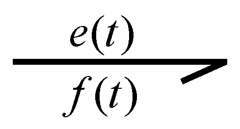
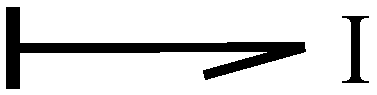
The bond graph methodology provides a modeling platform based on the exchange of power of the elements that form a system. Power is obtained as the product of two generalized power variables: effort $e\left(t\right)$ and flow $f\left(t\right)$, as shown in Figure 1.

In bond graph modeling, two generalized energy variables called momentum $p\left(t\right)={\int }_0^{t}e\left(\tau \right)d\tau$ and displacement $q\left(t\right)={\int }_0^{t}f\left(\tau \right)d\tau$ are used.

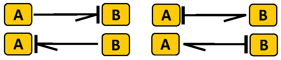
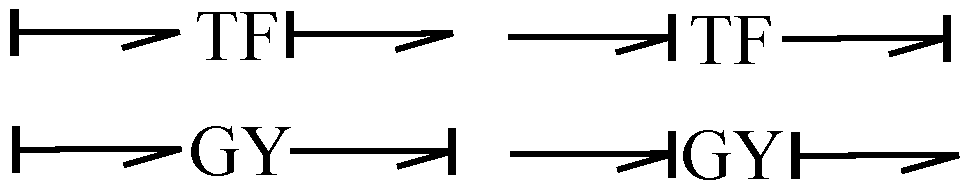
In order to obtain the sets of equations of a system, the constitutive relations of the elements are required. These relations can be dynamic or algebraic depending on the element and by the cause–effect assignment. In a bond graph, a bond with a causal stroke determines the causality assignment, and the assignments of the half arrow and the causal stroke are independent, as is shown in Figure 2.

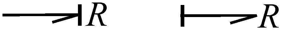
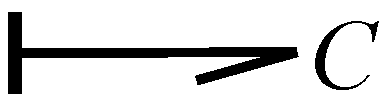
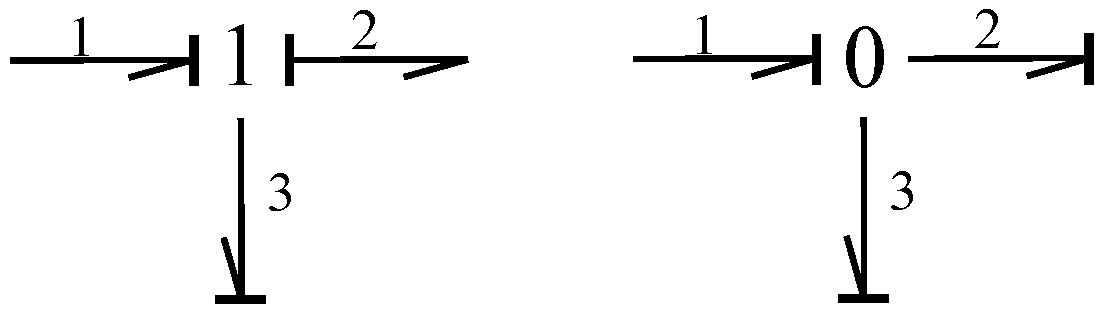
The different physical systems that can be used to build a dynamic system are described below:

• One-port passive elements are defined by:

  −

  Resistance taking whatever causality shown in Figure 3. This element represents damper, resistor, or fluid resistance, and the constitutive relationship is given by:

  $$e=Rf$$

  (21)

  Figure 3. Representation of a resistive bond.

  Figure 3. Representation of a resistive bond.

  −

  Capacitance in integral causality assignment where the flow variable is integrated to produce the effort variable, as illustrated in Figure 4. Accumulator, linear, and torsional springs represent capacitances whose constitutive relationship is described by:

  $$e=\frac{1}{C}\int fdt$$

  (22)

  Figure 4. Representation of a capacitive bond in integral causality.

  Figure 4. Representation of a capacitive bond in integral causality.

  This element in a derivative causality assignment is shown in Figure 5 and the corresponding constitutive relationship given by:

  $$f=C\frac{de}{dt}$$

  (23)

  Figure 5. Representation of a capacitive bond in derivative causality.

  Figure 5. Representation of a capacitive bond in derivative causality.

  −

  Inertance in integral causality assignment where the effort variable is integrated to produce the flow variable, which is shown in Figure 6. This element is representative of a mass, inductor, or flywheel, and its constitutive relationship is:

  $$f=\frac{1}{C}\int edt$$

  (24)

  Figure 6. Representation of an inductive bond in integral causality.

  Figure 6. Representation of an inductive bond in integral causality.

  When a derivative causality is assigned to this element, the constitutive relationship is described by:

  $$e=I\frac{df}{dt}$$

  (25)

  and Figure 7 shows this element with the causality applied.

  Figure 7. Representation of an inductive bond in derivative causality.

  Figure 7. Representation of an inductive bond in derivative causality.

• One-port active elements denoted by $\left(M{S}_e,M{S}_f\right)$ represent the power sources. These sources have only one causality, and this is shown in Figure 8;

  Figure 8. Representation of power sources: $M{S}_e$ is an effort source; $M{S}_f$ is a flow source.

  Figure 8. Representation of power sources: $M{S}_e$ is an effort source; $M{S}_f$ is a flow source.
• Two-port elements represent distribution elements denoted by $\left(TF,GY\right)$, which are transformers and gyrators, and Figure 9 shows these elements;

  Figure 9. Representation of transformers, $TF$, and gyrators, $GY$.

  Figure 9. Representation of transformers, $TF$, and gyrators, $GY$.
  The constitutive relationships for the transformers are given by:

  $$\begin{array}{ccc}\hfill e_1& =& a{e}_2\hfill \end{array}$$

  (26)

  $$\begin{array}{ccc}\hfill f_1& =& \frac{1}{a}{f}_2\hfill \end{array}$$

  (27)

  and for gyrators are:

  $$\begin{array}{ccc}\hfill e_1& =& b{f}_2\hfill \end{array}$$

  (28)

  $$\begin{array}{ccc}\hfill f_1& =& \frac{1}{b}{e}_2\hfill \end{array}$$

  (29)
• Three-port elements represent junctions and are denoted by $\left(1,0\right)$, which determine the different connections of the elements, and these junctions are shown in Figure 10;

  Figure 10. Connection representation: series junctions, 1, and parallel junctions, 0.

  Figure 10. Connection representation: series junctions, 1, and parallel junctions, 0.
  A one-junction is defined by:

  $$\begin{array}{ccc}\hfill e_{in1}+e_{in2}+\cdots +e_{inm}& =& e_{out1}+e_{out2}+\cdots +e_{outn}\hfill \end{array}$$

  (30)

  $$\begin{array}{ccc}\hfill f_{in1}& =& f_{in2}=\cdots =f_{inm}=f_{out1}=f_{out2}=\cdots =f_{outn}\hfill \end{array}$$

  (31)

  and for a zero-junction:

  $$\begin{array}{ccc}\hfill e_{in1}& =& e_{in2}=\cdots =e_{inm}=e_{out1}=e_{out2}=\cdots =e_{outn}\hfill \end{array}$$

  (32)

  $$\begin{array}{ccc}\hfill f_{in1}+f_{in2}+\cdots +f_{inm}& =& f_{out1}+f_{out2}+\cdots +f_{outn}\hfill \end{array}$$

  (33)

  where m and n are the entry and exit bonds to the one-junction.

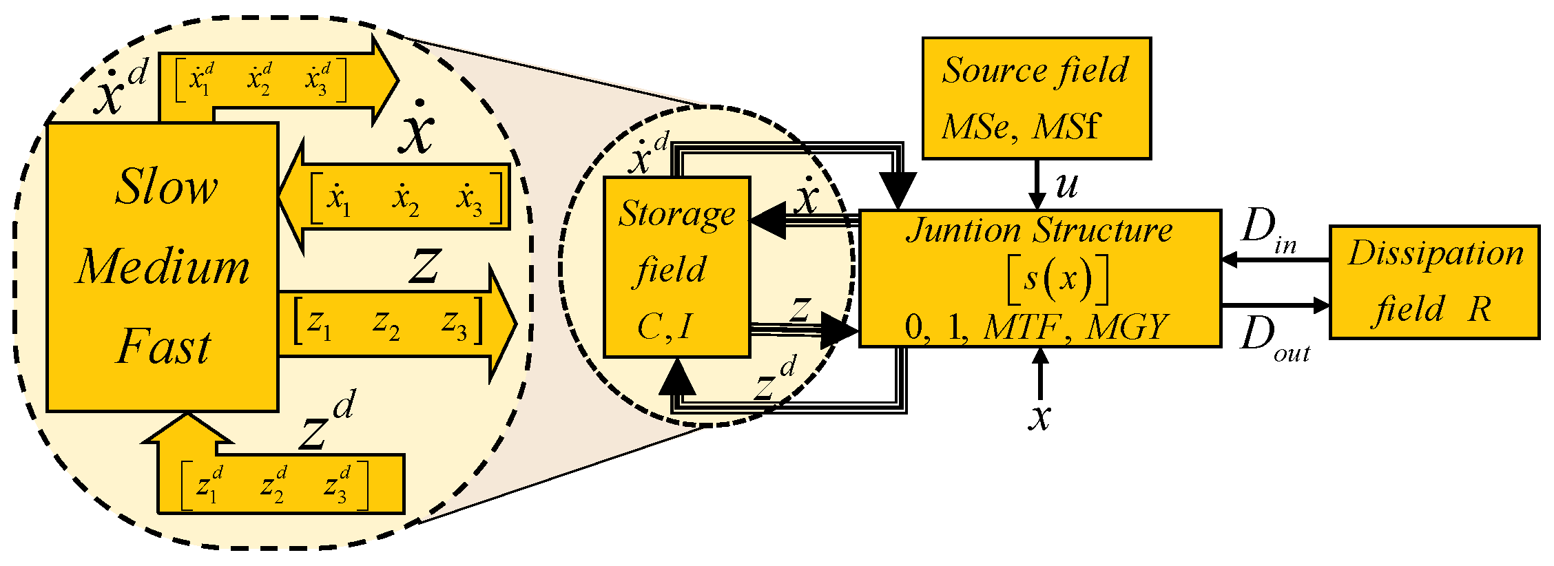
The different elements of a bond graph can be grouped into fields, and the use of junction structures allows relatively complex systems to be modeled and analyzed in this approach. A bond graph model with a preferred integral causality assignment (BGI) of a system with singular perturbations is shown in Figure 11. The junction structure of a bond graph model with three time scales is based on the junction structure of a basic bond graph model introduced in [30].

The block diagram of Figure 11 is described by:

• The source field denoted by $\left(M{S}_e,M{S}_f\right)$ that determines the plant input $u\left(t\right)\in {\Re }^p$;
• The junction structure denoted by $\left(0,1,MTF,MGY\right)$ with zero and one junctions, transformers $MTF$, and gyrators $MGY$, which can be modulated by state variables $x\left(t\right)$;
• The energy storage field denoted by $\left(C,I\right)$ that defines energy variables $q\left(t\right)$ and $p\left(t\right)$ associated with C and I storage elements in an integral causality assignment describing linearly independent state variables of energy $x\left(t\right)$ and co-energy $z\left(t\right)$ and storage elements with a derivative causality assigned describing linearly dependent state variables of energy $x^d\left(t\right)$ and co-energy $z^d\left(t\right)$.
  This storage field is defined by elements that represent the slow, medium, and fast dynamics that are indicated in Figure 11. The storage elements for each dynamic can have an integral causality whose state vector is $x\left(t\right)=\left[\begin{array}{c}{x}_1\left(t\right)\\ x_2\left(t\right)\\ x_3\left(t\right)\end{array}\right]$ and a derivative causality with state vector $x^d\left(t\right)=\left[\begin{array}{c}{x}_1^d\left(t\right)\\ x_2^d\left(t\right)\\ x_3^d\left(t\right)\end{array}\right]$.
  Therefore, the smallest circle in Figure 11 defines all the storage elements, and the largest circle indicates that this field is formed by the dynamics of three time scales. These dynamics are:

  −

  Slow dynamics $x_1\left(t\right)\in {\Re }^n$ and $x_1^d\left(t\right)\in {\Re }^{n_d}$ with constitutive relationships:

  $$\begin{array}{ccc}\hfill z_1\left(t\right)& =& F_1{x}_1\left(t\right)\hfill \end{array}$$

  (34)

  $$\begin{array}{ccc}\hfill z_1^d\left(t\right)& =& F_1^d{x}_1^d\left(t\right)\hfill \end{array}$$

  (35)

  −

  Medium dynamics $x_2\left(t\right)\in {\Re }^m$ and $x_2^d\left(t\right)\in {\Re }^{m_d}$ with constitutive relationships:

  $$\begin{array}{ccc}\hfill z_2\left(t\right)& =& F_2{x}_2\left(t\right)\hfill \end{array}$$

  (36)

  $$\begin{array}{ccc}\hfill z_2^d\left(t\right)& =& F_2^d{x}_2^d\left(t\right)\hfill \end{array}$$

  (37)

  −

  Fast dynamics $x_3\left(t\right)\in {\Re }^l$ and $x_3^d\left(t\right)\in {\Re }^{l_d}$ with constitutive relationships:

  $$\begin{array}{ccc}\hfill z_3\left(t\right)& =& F_3{x}_3\left(t\right)\hfill \end{array}$$

  (38)

  $$\begin{array}{ccc}\hfill z_3^d\left(t\right)& =& F_3^d{x}_3^d\left(t\right);\hfill \end{array}$$

  (39)

• The energy dissipation field denoted by $\left(R\right)$ that defines $D_{in}\left(t\right)\in {\Re }^r$ and $D_{out}\left(t\right)\in {\Re }^r$ as a mixture of power variables $e\left(t\right)$ and $f\left(t\right)$ indicating the energy exchanges between the dissipation field and the junction structure.

The mathematical model of the diagram in Figure 11 is obtained from the following lemma.

Lemma 1.

Consider a class of nonlinear systems of the type of product of state variables composed of three time scales modeled by bond graphs in a preferred integral causality assignment whose junction structure is defined by:

$$\left[\begin{array}{c}\stackrel{•}{x}\left(t\right)\\ D_{in}\left(t\right)\\ z^d\left(t\right)\end{array}\right]=\left[\begin{array}{cccc}{S}_{11}\left(x\right)& S_{12}\left(x\right)& S_{13}\left(x\right)& S_{14}\left(x\right)\\ S_{21}\left(x\right)& S_{22}\left(x\right)& S_{23}\left(x\right)& 0\\ S_{31}\left(x\right)& 0& 0& 0\end{array}\right]\left[\begin{array}{c}z\left(t\right)\\ D_{out}\left(t\right)\\ u\left(t\right)\\ {\stackrel{•}{x}}^d\left(t\right)\end{array}\right]$$

(40)

where the state variables are:

$$x\left(t\right)=\left[\begin{array}{c}{x}_1\left(t\right)\\ x_2\left(t\right)\\ x_3\left(t\right)\end{array}\right]$$

(41)

$x_1\left(t\right)$, $x_2\left(t\right)$, and $x_3\left(t\right)$ being the slow, medium, and fast dynamics, respectively, with linear constitutive relationships:

$$\begin{array}{ccc}\hfill z\left(t\right)& =& Fx\left(t\right)\hfill \end{array}$$

(42)

$$\begin{array}{ccc}\hfill z^d\left(t\right)& =& F^d{x}^d\left(t\right)\hfill \end{array}$$

(43)

$$\begin{array}{ccc}\hfill D_{out}\left(t\right)& =& L{D}_{in}\left(t\right)\hfill \end{array}$$

(44)

then a mathematical model of this system is given by:

$$\left[\begin{array}{c}{\stackrel{•}{x}}_1\left(t\right)\\ {\epsilon }_1{\stackrel{•}{x}}_2\left(t\right)\\ {\epsilon }_2{\stackrel{•}{x}}_3\left(t\right)\end{array}\right]=A\left(x\right)x\left(t\right)+B\left(x\right)u\left(t\right)$$

(45)

where:

$$\begin{array}{ccc}\hfill A\left(x\right)& =& \epsilon E^{-1}\left(x\right)\left[S_{11}\left(x\right)+S_{12}\left(x\right)M\left(x\right)S_{21}\left(x\right)+S_{14}\left(x\right){\left(F^d\right)}^{-1}{\stackrel{•}{S}}_{31}\left(x\right)\right]F\hfill \end{array}$$

(46)

$$\begin{array}{ccc}\hfill B\left(x\right)& =& \epsilon E^{-1}\left(x\right)\left[S_{13}\left(x\right)+S_{12}\left(x\right)M\left(x\right)S_{23}\left(x\right)\right]\hfill \end{array}$$

(47)

with:

$$\begin{array}{ccc}\hfill E\left(x\right)& =& I-S_{14}\left(x\right){\left(F^d\right)}^{-1}{S}_{31}\left(x\right)F\hfill \end{array}$$

(48)

$$\begin{array}{ccc}\hfill M\left(x\right)& =& L{\left[I-S_{22}\left(x\right)L\right]}^{-1}\hfill \end{array}$$

(49)

and:

$$\epsilon =diag\left\{I,F_2^{-1},F_3^{-1}\right\}$$

(50)

The proof is presented in Appendix A. The symmetry between graphical modeling in a bond graph and mathematical modeling in the state space through Lemma 1 is established.

In order to obtain the mathematical model with the conditions of this paper from a bond graph model of a class of nonlinear systems with singular perturbations, the following assumptions have to be considered.

Assumption 6.

The constitutive relationships of the storage elements and dissipation elements are linear.

Assumption 7.

The product of the state variables defines the class of nonlinear systems.

Assumption 8.

The relationships between storage elements in integral and derivative causality defined by $E\left(x\right)$ are structurally invertible.

Assumption 9.

The algebraic loops between dissipation elements defined by $M\left(x\right)$ are structurally invertible.

The bond graph methodology allows deriving different models depending on the causality applied to its elements. Furthermore, when a system has the properties of having different time scales, reduced models can be obtained. Therefore, the direct determination of reduced models for a class of nonlinear systems with three time scales in a bond graph approach is presented.

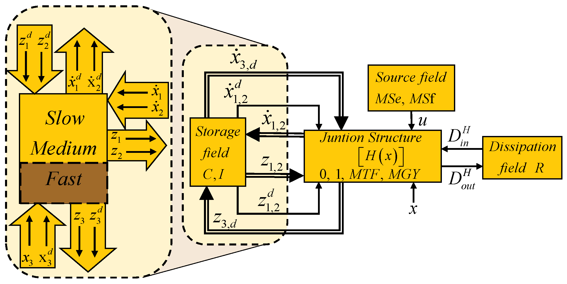
In the analysis of singularly perturbed systems, the fast dynamics reach the steady state when the medium and slow dynamics are developing their transitory period. These reduced models can be obtained by assigning a derivative causality to the storage elements of the fast dynamics and maintaining integral causality to the storage elements of the medium and slow dynamics. This formulation is proposed in Figure 12.

The junction structure of Figure 12 indicates that for the elements of the storage field of the slow and medium dynamics, an integral causality is assigned, which is denoted by $x_{1,2}$, and all the elements of the fast dynamics have a derivative causality, that is the elements that are in Figure 11 in integral causality $x_3$ and derivative $x_3^d$ will all have derivative causality and are denoted by $x_{3,d}$. Therefore, these key vectors are a compact representation of the storage field:

• $x_{1,2}$ state variables of slow and medium dynamics in integral causality;
• $x_{3,d}$ state variables linearly independent and dependent on fast dynamics in derivative causality.

The representation of the left part of Figure 12 shows individually the causality for each of the slow, medium, and fast dynamics. The causality of the dissipative field has to be adjusted with its key vectors $\left(D_{in}^H,D_{out}^H\right)$ so that the entire bond graph is causally corrected.

Based on the diagram in Figure 12, the junction structure that allows deriving the reduced models is introduced in the following lemma.

Lemma 2.

Consider a class of nonlinear systems with singular perturbations modeled by bond graphs where the storage elements that represent slow and medium dynamics have an integral causality assignment, and for the storage elements for the fast dynamics, a derivative causality is assigned, whose junction structure is defined by:

$$\left[\begin{array}{c}{\stackrel{•}{x}}_{1,2}\left(t\right)\\ z_{3,d}\left(t\right)\\ D_{in}^H\left(t\right)\\ z_{1,2}^d\left(t\right)\end{array}\right]=\left[\begin{array}{ccccc}{H}_{11}^{\left(1,2\right)\left(1,2\right)}\left(x\right)& H_{11}^{\left(1,2\right)\left(3,d\right)}\left(x\right)& H_{12}^{\left(1,2\right)}\left(x\right)& H_{13}^{\left(1,2\right)}\left(x\right)& H_{14}^{\left(1,2\right)}\left(x\right)\\ H_{11}^{\left(3,d\right)\left(1,2\right)}\left(x\right)& H_{11}^{\left(3,d\right)\left(3,d\right)}\left(x\right)& H_{12}^{\left(3,d\right)}\left(x\right)& H_{13}^{\left(3,d\right)}\left(x\right)& 0\\ H_{21}^{\left(1,2\right)}\left(x\right)& H_{21}^{\left(3,d\right)}\left(x\right)& H_{22}\left(x\right)& H_{23}\left(x\right)& 0\\ H_{31}^{\left(1,2\right)}\left(x\right)& 0& 0& 0& 0\end{array}\right]\left[\begin{array}{c}{z}_{1,2}\left(t\right)\\ {\stackrel{•}{x}}_{3,d}\left(t\right)\\ D_{out}^H\left(t\right)\\ u\left(t\right)\\ {\stackrel{•}{x}}_{1,2}^d\left(t\right)\end{array}\right]$$

(51)

where the state variables are expressed by:

$$x_{1,2}\left(t\right)=\left[\begin{array}{c}{x}_1\left(t\right)\\ x_2\left(t\right)\end{array}\right]$$

(52)

and:

$$x_{3,d}=\left[\begin{array}{c}{x}_3\left(t\right)\\ x_3^d\left(t\right)\end{array}\right]$$

(53)

with

$$D_{out}^H\left(t\right)=L_H{D}_{in}^H\left(t\right)$$

(54)

then the quasi-steady-state models are given by:

$$\left[\begin{array}{c}{\stackrel{•}{x}}_{1,2}\left(t\right)\\ x_{3,d}\left(t\right)\end{array}\right]=\left[\begin{array}{c}{A}^{\left(1,2\right)}\left(x\right)\\ A^{\left(3,d\right)\left(1,2\right)}\left(x\right)\end{array}\right]x_{1,2}\left(t\right)+\left[\begin{array}{c}{B}^{\left(1,2\right)}\left(x\right)\\ B^{\left(3,d\right)}\left(x\right)\end{array}\right]u\left(t\right)$$

(55)

where:

$$\begin{array}{ccc}\hfill A^{\left(1,2\right)}\left(x\right)& =& {\epsilon }_H{\left[E^{\left(1,2\right)}\left(x\right)\right]}^{-1}\left[H_{11}^{\left(1,2\right)\left(1,2\right)}\left(x\right)+H_{12}^{\left(1,2\right)}{N}_H\left(x\right)H_{21}^{\left(1,2\right)}\left(x\right)\right.\hfill \\ & & \left.+H_{14}^{\left(1,2\right)}\left(x\right){\left(F_{1,2}^d\right)}^{-1}{\stackrel{•}{H}}_{31}^{\left(1,2\right)}\left(x\right)\right]F_{1,2}\hfill \end{array}$$

(56)

$$\begin{array}{ccc}\hfill B^{\left(1,2\right)}\left(x\right)& =& {\epsilon }_H{\left[E^{\left(1,2\right)}\left(x\right)\right]}^{-1}\left[H_{13}^{\left(1,2\right)}\left(x\right)+H_{12}^{\left(1,2\right)}{N}_H\left(x\right)H_{23}^{\left(1,2\right)}\left(x\right)\right]\hfill \end{array}$$

(57)

$$\begin{array}{ccc}\hfill A^{\left(3,d\right)\left(1,2\right)}\left(x\right)& =& {\left(F_{3,d}\right)}^{-1}\left[H_{11}^{\left(3,d\right)\left(1,2\right)}\left(x\right)+H_{12}^{\left(3,d\right)}{N}_H\left(x\right)H_{21}^{\left(1,2\right)}\left(x\right)\right]\hfill \end{array}$$

(58)

$$\begin{array}{ccc}\hfill B^{\left(3,d\right)}\left(x\right)& =& {\left(F_{3,d}\right)}^{-1}\left[H_{13}^{\left(3,d\right)}\left(x\right)+H_{12}^{\left(3,d\right)}{N}_H\left(x\right)H_{23}\left(x\right)\right]\hfill \end{array}$$

(59)

with:

$$\begin{array}{ccc}\hfill N_H\left(x\right)& =& L_H{\left[I-H_{22}\left(x\right)L_H\right]}^{-1}\hfill \end{array}$$

(60)

$$\begin{array}{ccc}\hfill E^{\left(1,2\right)}\left(x\right)& =& I-H_{14}^{\left(1,2\right)}\left(x\right){\left(F_{1,2}^d\right)}^{-1}{H}_{31}^{\left(1,2\right)}\left(x\right)F_{1,2}\hfill \end{array}$$

(61)

and:

$$\begin{array}{ccc}\hfill F_{1,2}& =& diag\left\{F_1,F_2\right\}\hfill \end{array}$$

(62)

$$\begin{array}{ccc}\hfill F_{1,2}^d& =& diag\left\{F_1^d,F_2^d\right\}\hfill \end{array}$$

(63)

$$\begin{array}{ccc}\hfill F_{3,d}& =& diag\left\{F_3,F_3^d\right\}\hfill \end{array}$$

(64)

$$\begin{array}{ccc}\hfill {\epsilon }_H& =& diag\left\{I,F_2^{-1}\right\}\hfill \end{array}$$

(65)

The proof is presented in Appendix B.

The model described by Lemma 2 represents a system in which the fast dynamics has converged. However, in an analysis at a time greater than the convergence of the medium dynamics, reduced models can be obtained.

The application of Lemma 2 requires that the following assumptions be satisfied.

Assumption 10.

The equation:

$$A_{31}\left(x\right)\overline{x_1}\left(t\right)+A_{32}\left(x\right)\overline{x_2}\left(t\right)+A_{33}\left(x\right)\overline{x_3}\left(t\right)+B_3\left(x\right)u\left(t\right)=0$$

(66)

can be solved in terms of:

$$\overline{x_3}\left(t\right)=\overline{{\varphi }_i}\left(\overline{x_1},\overline{x_2},u\right),i=1,2,\cdots ,k$$

(67)

where k are distinct roots.

Assumption 11.

The $A_{33}\left(x\right)$ matrix is nonsingular.

Assumption 12.

The algebraic loops matrix $N_H\left(x\right)$ is nonsingular.

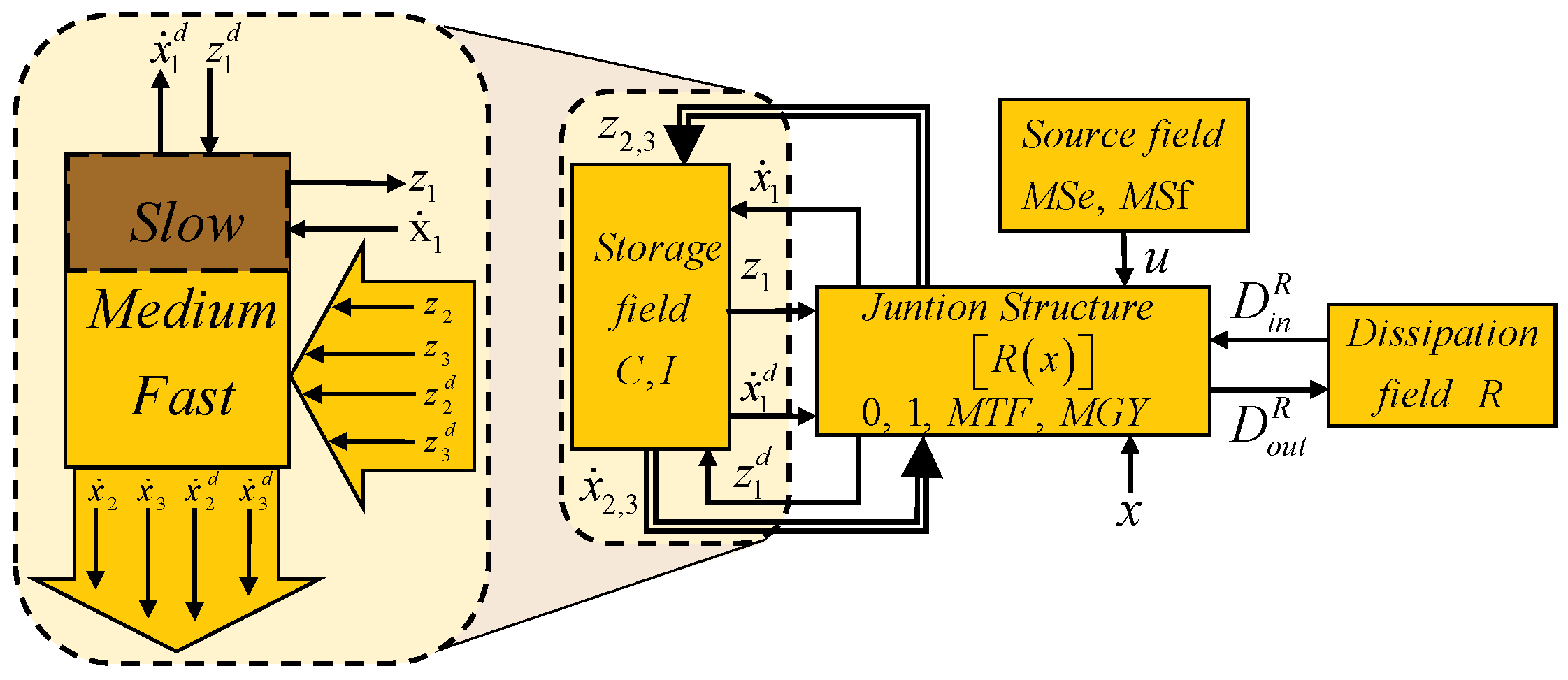
This new model reduced in a bond graph approach is obtained by assigning derivative causality to the storage elements of the medium and fast dynamics and to the storage elements of the slow dynamics, and an integral causality is assigned. This last reduction is illustrated in Figure 13.

The junction structure of Figure 13 indicates that all the storage elements of the medium and fast dynamics have derivative causality in compact form denoted by $x_{2,3}$, and for the linearly independent elements of the slow dynamics defined by $x_1$, an integral causality is assigned. The left part of Figure 13 shows the causality assignment for each dynamics of the system. Due to the change of causalities in the elements described, the causality in the dissipation elements will have to be adjusted through the key vectors $\left(D_{in}^R,D_{out}^R\right)$ so that the bond graph is causally correct.

The mathematical model according to Figure 13 is obtained by applying the following lemma.

Lemma 3.

Consider a class of nonlinear singularly perturbed systems modeled by bond graphs where for the storage elements that determine the slow dynamics, an integral causality is assigned, and the storage elements for the medium and fast dynamics have a derivative causality assignment with a junction structure defined by:

$$\left[\begin{array}{c}{\stackrel{•}{x}}_1\left(t\right)\\ z_{2,3}\left(t\right)\\ D_{in}^R\left(t\right)\\ z_1^d\left(t\right)\end{array}\right]=\left[\begin{array}{ccccc}{R}_{11}^{11}\left(x\right)& R_{11}^{1\left(2,3\right)}\left(x\right)& R_{12}^{11}\left(x\right)& R_{13}^{11}\left(x\right)& R_{14}^{11}\left(x\right)\\ R_{11}^{\left(2,3\right)1}\left(x\right)& R_{11}^{\left(2,3\right)\left(2,3\right)}\left(x\right)& R_{12}^{\left(2,3\right)}\left(x\right)& R_{13}^{\left(2,3\right)}\left(x\right)& 0\\ R_{21}^{11}\left(x\right)& R_{11}^{\left(2,3\right)}\left(x\right)& R_{22}\left(x\right)& R_{23}\left(x\right)& 0\\ R_{31}^{11}\left(x\right)& 0& 0& 0& 0\end{array}\right]\left[\begin{array}{c}{z}_1\left(t\right)\\ {\stackrel{•}{x}}_{2,3}\left(t\right)\\ D_{out}^R\left(t\right)\\ u\left(t\right)\\ {\stackrel{•}{x}}_1^d\left(t\right)\end{array}\right]$$

(68)

where the state variables for the medium and fast dynamics are described by:

$$x_{2,3}\left(t\right)=\left[\begin{array}{c}{x}_2\left(t\right)\\ x_2^d\left(t\right)\\ x_3\left(t\right)\\ x_3^d\left(t\right)\end{array}\right]$$

(69)

with

$$D_{out}^R\left(t\right)=L_R{D}_{in}^R\left(t\right)$$

(70)

then the quasi-steady-state models are given by:

$$\begin{array}{ccc}\hfill \stackrel{•}{\widetilde{x_1}}\left(t\right)& =& \widetilde{A_{11}}\left(x\right)\widetilde{x_1}\left(t\right)+\widetilde{B_1}\left(x\right)u\left(t\right)\hfill \end{array}$$

(71)

$$\begin{array}{ccc}\hfill \widetilde{x_{2,3}}\left(t\right)& =& \widetilde{A_{23}}\left(x\right)\widetilde{x_1}\left(t\right)+\widetilde{B_{2,3}}\left(x\right)u\left(t\right)\hfill \end{array}$$

(72)

where:

$$\begin{array}{ccc}\hfill \widetilde{A_{11}}\left(x\right)& =& {\widetilde{E_1}}^{-1}\left(x\right)\left[R_{11}^{11}\left(x\right)+R_{12}^{11}\left(x\right)N_R\left(x\right)R_{21}^{11}\left(x\right)+R_{14}^{11}\left(x\right){\left(F_1^d\right)}^{-1}{\stackrel{•}{R}}_{31}^{11}\left(x\right)\right]F_1\hfill \end{array}$$

(73)

$$\begin{array}{ccc}\hfill \widetilde{A_{23}}& =& F_{2,3}^{-1}\left[R_{11}^{\left(2,3\right)1}\left(x\right)+R_{12}^{\left(2,3\right)}{N}_R\left(x\right)R_{21}^{11}\left(x\right)\right]F_1\hfill \end{array}$$

(74)

$$\begin{array}{ccc}\hfill \widetilde{B_1}\left(x\right)& =& {\widetilde{E_1}}^{-1}\left(x\right)\left[R_{13}^{11}\left(x\right)+R_{12}^{11}\left(x\right)N_R\left(x\right)R_{23}\left(x\right)\right]\hfill \end{array}$$

(75)

$$\begin{array}{ccc}\hfill \widetilde{B_{2,3}}\left(x\right)& =& F_{2,3}^{-1}\left[R_{13}^{\left(2,3\right)}\left(x\right)+R_{12}^{\left(2,3\right)}{N}_R\left(x\right)R_{23}\left(x\right)\right]F_1\hfill \end{array}$$

(76)

with:

$$\begin{array}{ccc}\hfill N_R\left(x\right)& =& L_R{\left[I-R_{22}\left(x\right)L_R\right]}^{-1}\hfill \end{array}$$

(77)

$$\begin{array}{ccc}\hfill F_{2,3}& =& diag\left\{F_2,F_3\right\}\hfill \end{array}$$

(78)

The proof is presented in Appendix C.

The application of Lemma 3 requires that the following assumptions be satisfied.

Assumption 13.

The equation:

$$A_{21}\left(x\right)\overline{x_1}\left(t\right)+A_{22}\left(x\right)\overline{x_2}\left(t\right)+A_{23}\left(x\right)\overline{x_3}\left(t\right)+B_2\left(x\right)u\left(t\right)=0$$

(79)

can be solved in terms of:

$$\overline{x_2}\left(t\right)=\overline{{\varphi }_i}\left(\overline{x_1},u\right),i=1,2,\cdots ,k$$

(80)

where k are distinct roots.

Assumption 14.

The $A_{22}\left(x\right)$ matrix is nonsingular.

Assumption 15.

The algebraic loops matrix $N_R\left(x\right)$ is nonsingular.

The reduced models of a system with singular perturbations can be obtained by applying Lemmas 2 and 3, determining a symmetry with the exact models for each of the dynamics.

The most important limitation of this paper is if the fast and medium dynamics’ storage elements cannot accept derivative causality due to the configuration of the model. A possible solution to this problem is to include dissipative elements with small or large numerical values in order to be able to assign derivative causality to the storage elements for fast and medium dynamics. Other limitations are that the given assumptions cannot be applied.

The proposed methodology was applied to the following case study.

4. Case Study as an Illustrative Example

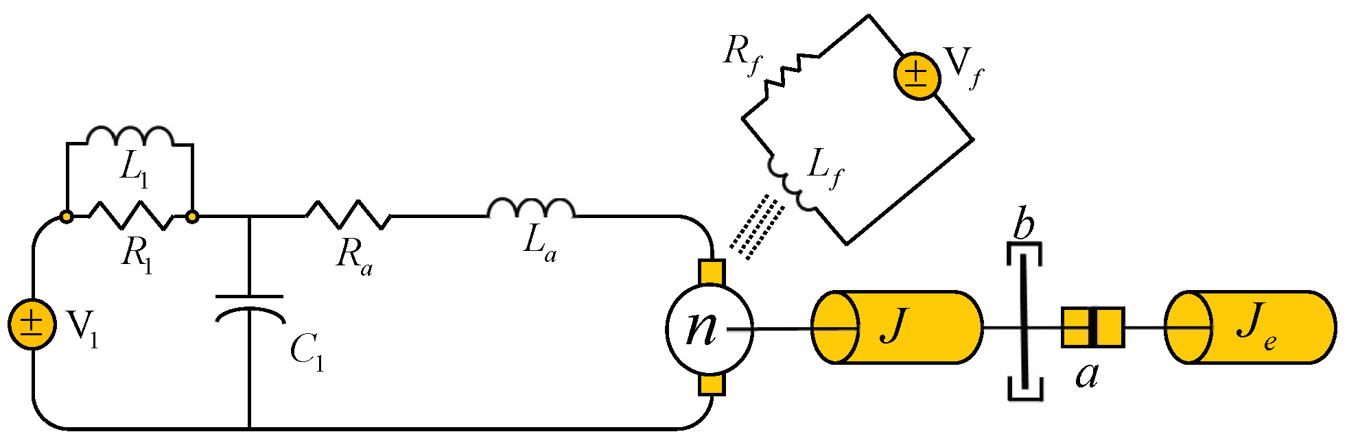
DC motors represent electromechanical systems that are widely used as actuating elements in industrial applications, whose advantages are easy speed and position control and a wide adjustability range. In the modeling of a DC motor, it is common to neglect nonlinearities in order to find a simple model. However, the assumption that the nonlinear elements on the system are negligible may give to big modeling errors. Likewise, it is common for the supply of energy to the DC motor to be obtained through the activation of elements of fast reaction electronics.

Therefore, the complete system will have three times scales and qualify as a singularly perturbed nonlinear system shown in Figure 14.

In Figure 14, $R_1,$ $L_1$, and $C_1$ represent the resistance, inductance, and capacitance, respectively, from the electronic input stage through which the supply voltage $V_1$ is introduced to the system. The armature winding is defined by the resistance $R_a$ and the inductance $L_a$; $R_f$ and $L_f$ are the resistance and inductance of the field winding with the voltage $V_f$ applied to this circuit. The mechanical load to the motor is the connection of two inertias J and $J_e$ by using a transformer a and a damping b.

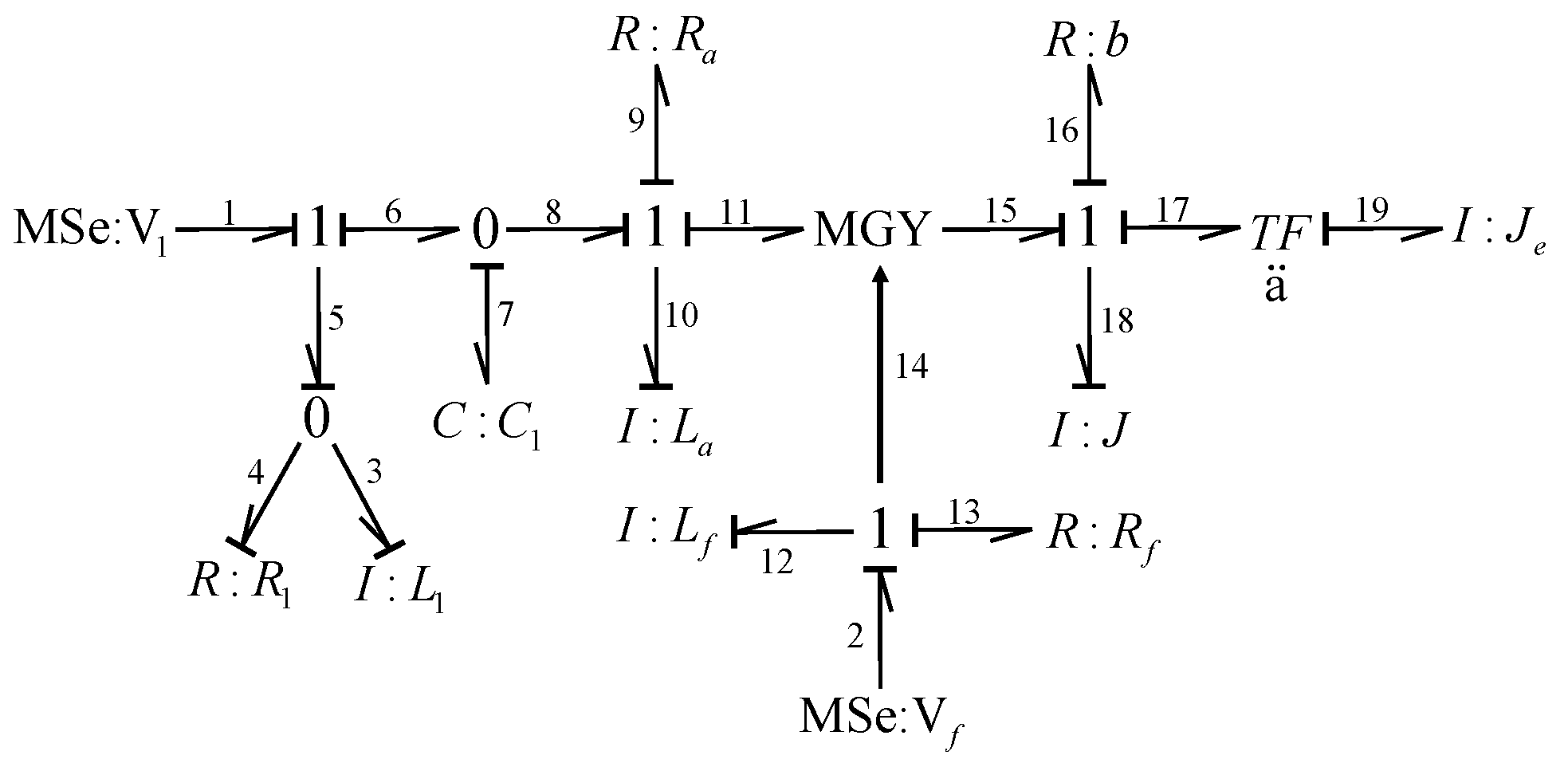
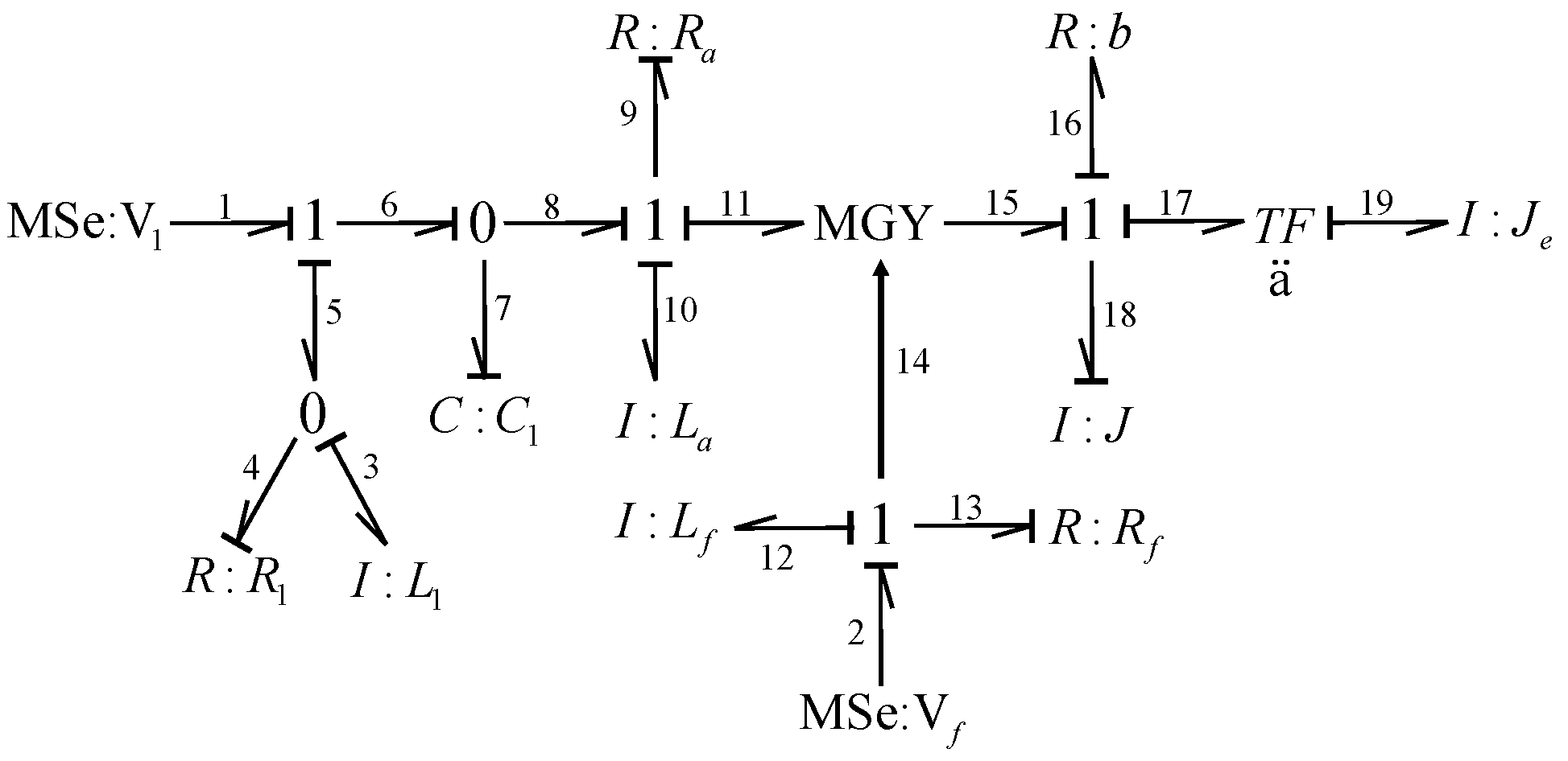
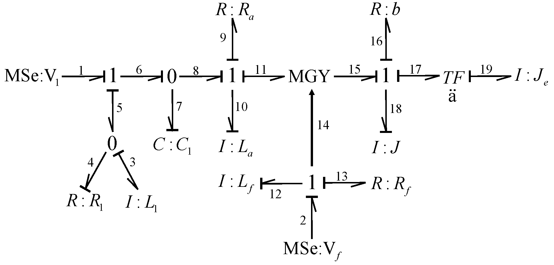
The bond graph in an integral causality assignment of the system is shown in Figure 15.

The bond graph in integral causality assignment allows obtaining the mathematical model of the complete system using Lemma 1, the first step being the description of the dynamics that form the system. The variables of the mechanical subsystem describe the slow dynamics expressed by the key vectors and constitutive relationship:

$$\begin{array}{ccc}\hfill x_1\left(t\right)& =& p_{18};{\stackrel{•}{x}}_1\left(t\right)=e_{18};z_1\left(t\right)=f_{18}\hfill \end{array}$$

(81)

$$\begin{array}{ccc}\hfill F_1& =& \frac{1}{J}\hfill \end{array}$$

(82)

and the key vectors for $I:J_e$ with a derivative causality assignment that determines a linearly dependent state variable are the following:

$$\begin{array}{ccc}\hfill x_1^d\left(t\right)& =& p_{20};{\stackrel{•}{x}}_1^d\left(t\right)=e_{20};z_1^d\left(t\right)=f_{20}\hfill \end{array}$$

(83)

$$\begin{array}{ccc}\hfill F_1^d& =& \frac{1}{J_e}\hfill \end{array}$$

(84)

The medium dynamics are represented by the storage elements of the electrical subsystem of the DC motor, whose key vectors and constitutive relationship are:

$$\begin{array}{ccc}\hfill x_2\left(t\right)& =& \left[\begin{array}{c}{p}_{10}\\ p_{12}\end{array}\right];{\stackrel{•}{x}}_2\left(t\right)=\left[\begin{array}{c}{e}_{10}\\ e_{12}\end{array}\right];z_2\left(t\right)=\left[\begin{array}{c}{f}_{10}\\ f_{12}\end{array}\right]\hfill \end{array}$$

(85)

$$\begin{array}{ccc}\hfill F_2& =& diag\left\{\frac{1}{L_a},\frac{1}{L_f}\right\}\hfill \end{array}$$

(86)

The electronic subsystem for supplying power to the motor represents the fast dynamics defined by:

$$\begin{array}{ccc}\hfill x_3\left(t\right)& =& \left[\begin{array}{c}{p}_3\\ q_7\end{array}\right];{\stackrel{•}{x}}_2\left(t\right)=\left[\begin{array}{c}{e}_3\\ f_7\end{array}\right];z_2\left(t\right)=\left[\begin{array}{c}{f}_3\\ e_7\end{array}\right]\hfill \end{array}$$

(87)

$$\begin{array}{ccc}\hfill F_3& =& diag\left\{\frac{1}{L_1},\frac{1}{C_1}\right\}\hfill \end{array}$$

(88)

according to Figure 11 for the dissipation elements:

$$\begin{array}{ccc}\hfill D_{in}\left(t\right)& =& \left[\begin{array}{c}{f}_{16}\\ f_9\\ f_{13}\\ e_4\end{array}\right];D_{out}\left(t\right)=\left[\begin{array}{c}{e}_{16}\\ e_9\\ e_{13}\\ f_4\end{array}\right]\hfill \end{array}$$

(89)

$$\begin{array}{ccc}\hfill L& =& diag\left\{b,R_a,R_f,\frac{1}{R_1}\right\}\hfill \end{array}$$

(90)

and the inputs:

$$u\left(t\right)=\left[\begin{array}{c}{e}_1\\ e_2\end{array}\right]$$

(91)

The system order is given by $n=1$, $n_d=1$, $m=2$, and $l=2$; thus, $n+m+l=5$ and $F=diag\left\{F_1,F_2,F_3\right\}$. The junction structure $S\left(x\right)$ is described by:

$$\left[\begin{array}{c}{e}_{18}\\ e_{10}\\ e_{12}\\ e_3\\ f_7\\ f_{16}\\ f_9\\ f_{13}\\ e_4\\ f_{20}\end{array}\right]=\left[\begin{array}{cccccccccccc}0& f_{12}& 0& 0& 0& -1& 0& 0& 0& 0& 0& -a\\ -f_{12}& 0& 0& 0& 1& 0& -1& 0& 0& 0& 0& 0\\ 0& 0& 0& 0& 0& 0& 0& -1& 0& 0& 1& 0\\ 0& 0& 0& 0& -1& 0& 0& 0& 0& 1& 0& 0\\ 0& -1& 0& 1& 0& 0& 0& 0& 1& 0& 0& 0\\ 1& 0& 0& 0& 0& 0& 0& 0& 0& 0& 0& 0\\ 0& 1& 0& 0& 0& 0& 0& 0& 0& 0& 0& 0\\ 0& 0& 1& 0& 0& 0& 0& 0& 0& 0& 0& 0\\ 0& 0& 0& 0& -1& 0& 0& 0& 0& 1& 0& 0\\ a& 0& 0& 0& 0& 0& 0& 0& 0& 0& 0& 0\end{array}\right]\left[\begin{array}{c}{f}_{18}\\ f_{10}\\ f_{12}\\ f_3\\ e_7\\ e_{16}\\ e_9\\ e_{13}\\ f_4\\ e_1\\ e_2\\ e_{20}\end{array}\right]$$

(92)

From (40), (48), (82), (84), and (92), the relationship of the linearly dependent state variable to the linearly independent variable is described by:

$$E\left(x\right)=diag\left\{1+a^2\frac{J_e}{J},I_4\right\}$$

(93)

From (45)–(47), and (49) with (82), (86), (88), and (93), the mathematical model of the complete system is given by:

$$\left[\begin{array}{c}{\stackrel{•}{x}}_1\left(t\right)\\ {\epsilon }_1{\stackrel{•}{x}}_2\left(t\right)\\ {\epsilon }_2{\stackrel{•}{x}}_3\left(t\right)\end{array}\right]=\left[\begin{array}{ccccc}\frac{-b}{J+a^2{J}_e}& \frac{J}{J+a^2{J}_e}·\frac{p_{12}}{L_f{L}_a}& 0& 0& 0\\ \frac{-L_a{p}_{12}}{J{L}_f}& -R_a& 0& 0& \frac{L_a}{C_1}\\ 0& 0& -R_f& 0& 0\\ 0& 0& 0& 0& \frac{-L_1}{C_1}\\ 0& \frac{-C_1}{L_a}& 0& \frac{C_1}{L_1}& \frac{-1}{R_1}\end{array}\right]x\left(t\right)+\left[\begin{array}{cc}0& 0\\ 0& 0\\ 0& L_f\\ L_1& 0\\ \frac{C_1}{R_1}& 0\end{array}\right]u\left(t\right)$$

(94)

Assigning a derivative causality to all the storage elements $\left(I:L_1;C:C_1\right)$ that represent the fast dynamics $\left(x_3\right)$ and maintaining integral causality to the elements of the medium and slow state variables $\left(I:L_a;I:L_f\right)$ and $\left(I:J\right)$, respectively, the reduced model (15) applying Lemma 2 is obtained. Figure 16 shows the bond graph to obtain the reduced model when the fast dynamics have converged.

In this case, the dissipation elements retain the same causality with respect to the bond graph of Figure 13, then the key vectors and their constitutive relationship are defined by:

$$D_{in}^H\left(t\right)=D_{in}\left(t\right);D_{out}^H\left(t\right)=D_{out}\left(t\right);L_H=L$$

(95)

Applying Lemma 2, the junction structure of the bond graph of Figure 14 is given by:

(96)

From (56), (57), (60), and (61) with (96), the quasi-steady-state model for $x_1$ and $x_2$ is defined by:

$${\stackrel{•}{x}}_{1,2}\left(t\right)=\left[\begin{array}{ccc}\frac{-b}{J+a^2{J}_e}& \frac{p_{12}}{L_a{L}_f\left(J+a^2{J}_e\right)}& 0\\ \frac{-p_{12}}{J{L}_f}{L}_a& -R_a& 0\\ 0& 0& -R_f\end{array}\right]x_{1,2}\left(t\right)+\left[\begin{array}{cc}0& 0\\ 1& 0\\ 0& 1\end{array}\right]u\left(t\right)$$

(97)

From (58)–(60) with (96), the expression of the fast dynamics when they have converged is described by:

$$x_{3,d}\left(t\right)=\left[\begin{array}{ccc}0& \frac{L_1}{L_a}& 0\\ 0& 0& 0\end{array}\right]x_{1,2}\left(t\right)+\left[\begin{array}{cc}0& 0\\ C_1& 0\end{array}\right]u\left(t\right)$$

(98)

The smallest model is obtained by assigning derivative causality to the storage elements $\left(I:L_a;I:L_f\right)$ of the medium dynamics $\left(x_2\right)$, which is shown in Figure 17.

In order to have a correct bond graph, the key vectors and the constitutive relation for the dissipation elements are defined by:

$$D_{in}^R\left(t\right)=\left[\begin{array}{c}{f}_{16}\\ e_9\\ e_{13}\\ e_4\end{array}\right];D_{out}^R\left(t\right)=\left[\begin{array}{c}{e}_{16}\\ f_9\\ f_{13}\\ f_4\end{array}\right];L_R=diag\left\{b,\frac{1}{R_a},\frac{1}{R_f},\frac{1}{R_1}\right\}$$

(99)

and the junction structure is obtained by:

(100)

The quasi-steady-state model applying Lemma 3 is obtained from (73), (75), and (77) with (100) given by:

$$\stackrel{•}{\widetilde{x_1}}\left(t\right)=\left(\frac{1}{J+a^2{J}_e}\right)\left(\frac{-b}{J}-\frac{p_{12}^2}{J{L}_f^2{R}_a}\right)\widetilde{x_1}\left(t\right)+\left(\frac{J}{J+a^2{J}_e}\right)\left[\begin{array}{cc}\frac{p_{12}}{L_f{R}_a}& 0\end{array}\right]u\left(t\right)$$

(101)

The convergence of the medium and fast dynamics is determined from (74), (76), and (77) with (100) expressed as:

$$\widetilde{x_{2,3}}\left(x\right)=\left[\begin{array}{c}\frac{-p_{12}{L}_a}{J{L}_f{L}_a}\\ 0\\ \frac{-p_{12}{L}_1}{J{L}_f{L}_a}\\ 0\end{array}\right]\widetilde{x_1}\left(t\right)+\left[\begin{array}{cc}\frac{L_a}{R_a}& 0\\ 0& \frac{L_f}{R_f}\\ \frac{L_1}{R_a}& \frac{-L_1}{R_1}\\ C_1& 0\end{array}\right]u\left(t\right)$$

(102)

In order to show the effectiveness of the proposed methodology,

Table 1. Parameters of the case study.

$R_1$ = 100 Ω	$L_f$ = 0.02 F	$a=2$
$R_f$ = 10 Ω	$b$ = 1.2 N-m-s	$V_a$ = 120 V
$R_a$ = 25 Ω	$J$ = 3.5 N-m-s2	$V_f$ = 24 V
$L_1$ = 10 μH	$J_e$ = 5 N-m-s2
$L_e$ = 0.1 H	$C_1$ = 1 μF

gives the numerical parameters of the bond graph illustrated in Figure 15.

In order to verify numerically the reduced models with respect to the exact model, the graphs are illustrated in the following figures. The simulation of this case study was obtained by using the 20-sim software.

It is important to note that the simulation results for the exact model shown in Figure 15 were obtained directly from the bond graph library of the 20-sim software. However, the simulation of the reduced model was carried out through Equations (97) and (98) for the convergence of the fast dynamics. The simulation of the reduced model for the convergence of the medium and fast dynamics was used in Equations (101) and (102).

Figure 18 shows the behavior of the fast state variables, based on the exact model $\left(p_3,q_7\right)$ and the reduced model $\left(\overline{p_3},\overline{q_7}\right)$ given by (98).

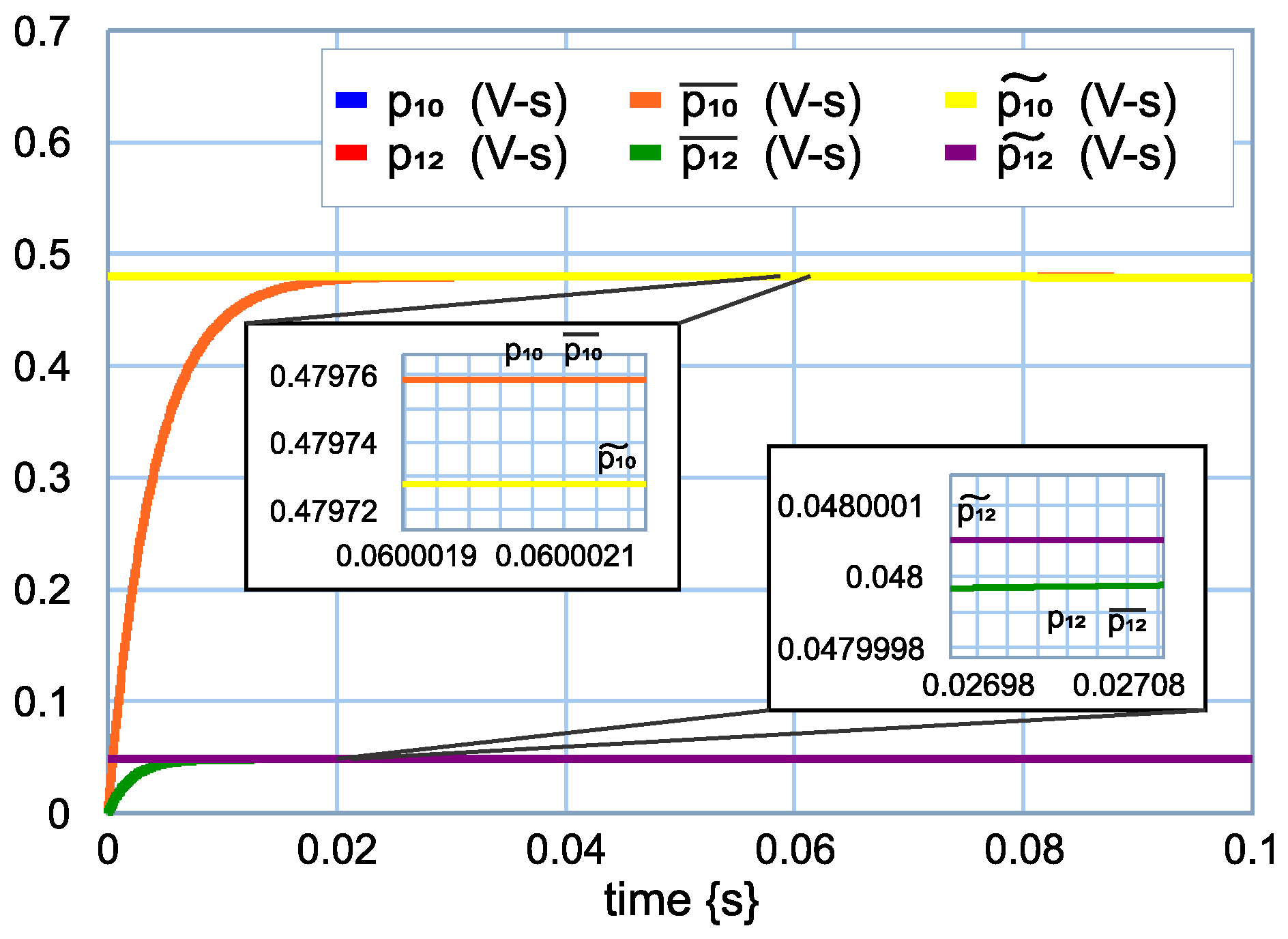
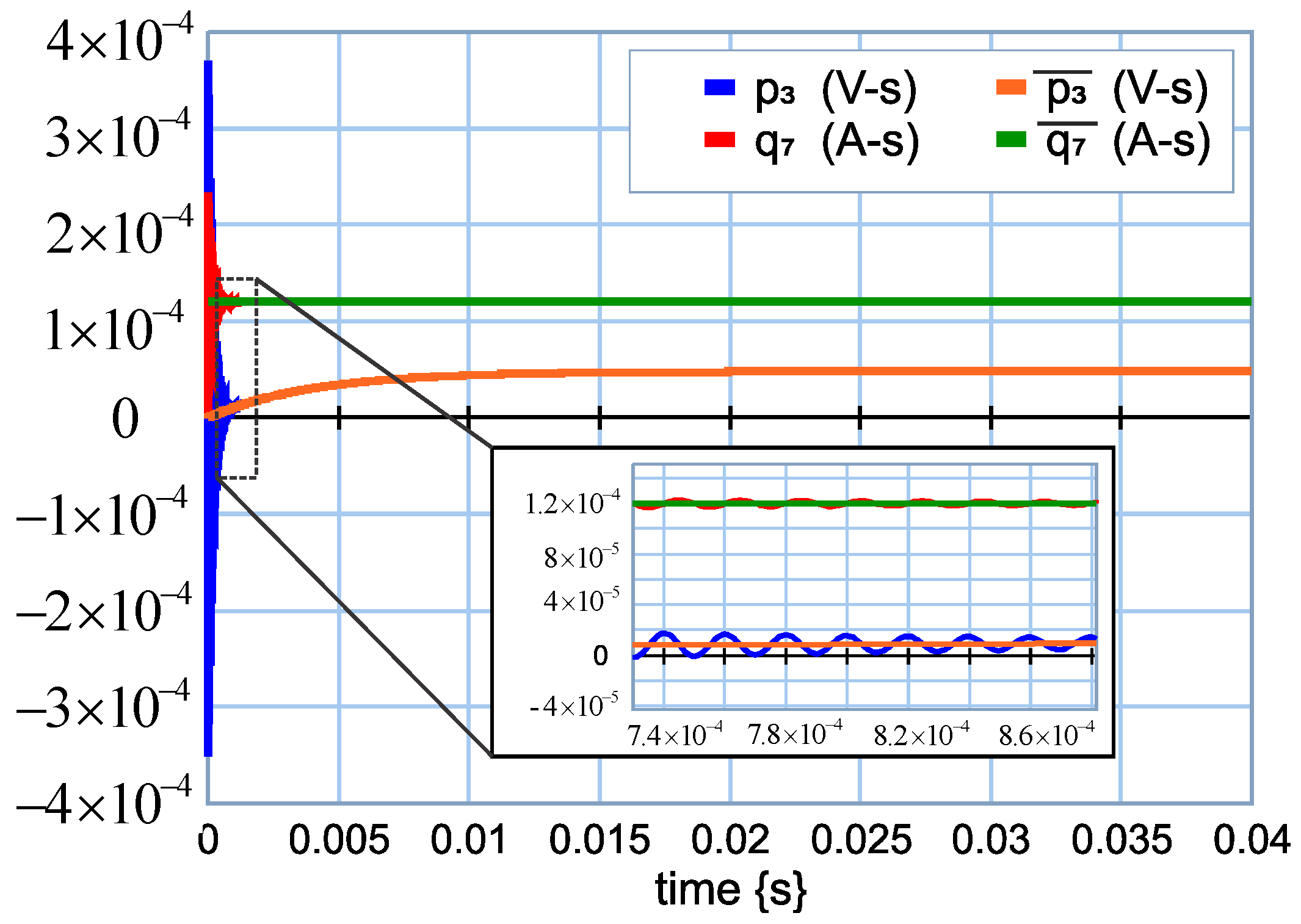
Now, the performance of the state variables of the medium dynamics is shown in Figure 19. The great closeness of the models reduced to the exact model can be seen.

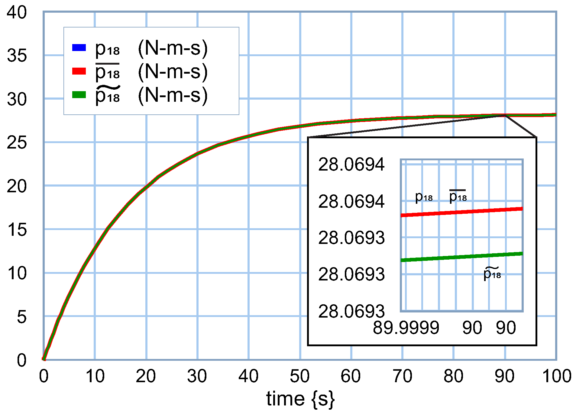
Finally, the behavior of the state variable of the slow dynamics is illustrated in Figure 20.

It is clear from Figure 18, Figure 19 and Figure 20 that the system contains three time scales: the simulation time for the convergence of the fast dynamics is from 0–0.015 s, of the medium dynamics from 0–0.03 s, and of the slow dynamics from 0–100 s.

This paper can be applied to multidisciplinary systems, for example mechatronics, electric vehicles [29], and chemical processes [15], where they are characterized by having several time scales in their dynamic behavior.

Some complex dynamical systems have been modeled in bond graphs, for example [31,32,33], and the possible application of this paper requires that the system contains several time scales and the class of nonlinear systems be according to the product of the state variables.

5. Conclusions

The analysis of a class of nonlinear systems with singular perturbations in a bond graph approach was presented. The type of systems, although they are specific, can be found in many electrical machines, as well as in aeronautical systems. One of the main objectives of singularly perturbed systems is to obtain simplified models. Therefore, reduced models in the physical domain have been proposed. The key for the direct determination of these models is to assign derivative causality to the storage elements that converge to their steady-state value, and for the remaining dynamics, an integral causality is assigned. In this way, the three time scales (fast, medium, slow) are reduced to two time scales (medium, slow) and finally to one (slow). The proposed methodology was applied to an electromechanical system, obtaining the reduced models, and the simulation results were shown, verifying the effectiveness of the presented lemmas.

Through this paper, the direct simulation of the bond graphs for reduced models is a challenge to achieve using the bond graph library of the 20-sim software, but it is required as future work to have these objectives.

Finally, the symmetry of graphical and mathematical models was established for systems modeled in a bond graph. Furthermore, reduced models from exact models for systems on three time scales by determining symmetries were presented.

References

1. Kokotovic, P.V.; Khalil, H.K.; O’Reilly, J. Singular Perturbation Methods in Control: Analysis and Design; Academic Press: London, UK, 1986. [Google Scholar]
2. Naidu, D.S. Singular Perturbation Methodology in Control Systems; IET: London, UK, 1988. [Google Scholar]
3. Silva-Madriz, R.; Sastry, S.S. Multiple Time Scales for Nonlinear Systems. Circuits Syst. Sygnal Process 1986, 5, 153–169. [Google Scholar] [CrossRef]
4. Su, W.C.; Gajic, Z.; Shen, X.M. The Exact Slow-Fast Decomposition of the Alegbraic Riccati Equation of Singularly Perturbed Systems. IEEE Trans. Autom. Control 1992, 37, 1456–1459. [Google Scholar] [CrossRef]
5. Fayaz, A.M. An interpolation method for the control of ε-varying Singularly Perturbed Systems. In Proceedings of the 40th IEEE Conference on Decision and Control, Orlando, FL, USA, 4–7 December 2001. [Google Scholar]
6. Hajer Bouzaouache, N.; Brajek, B. On guaranteed global exponential stability of polynomial singularly perturbed control systems. In Proceedings of the IMACS Multiconference on Computational Engineering in Systems Applications, Beijing, China, 4–6 October 2006. [Google Scholar]
7. Javid, S.H. Uniform Asymptotic Stability of Linear Time-Varying Singularly Perturbed Systems. J. Frankl. Inst. 1978, 305, 27–37. [Google Scholar] [CrossRef]
8. Javid, S.H. Stabilization of Time-Varying Singularly Perturbed Systems by Observer-Based Slow-State Feedback. IEEE Trans. Autom. Control 1982, 27, 702–704. [Google Scholar] [CrossRef]
9. Javid, S.H. Observing the Slow States of a Singularly Perturbed System. IEEE Trans. Autom. Control 1980, 25, 277–280. [Google Scholar] [CrossRef]
10. Sandell, N.R., Jr. Robust Stability of Systems with Application to Singular Perturbations. Automatica 1979, 15, 467–470. [Google Scholar] [CrossRef]
11. Esteban, S.; Aracil, J.; Gordillo, F. Three-Time Scale Singular Perturbation Control for a Radio-Control Helicopter on a Platform. In Proceedings of the AIAA Atmospheric Flight Mechanics Conference and Exhibit, San Francisco, CA, USA, 15–18 August 2005; pp. 1–19. [Google Scholar]
12. Munje, R.K.; Musmade, B.B.; Parkhe, J.G.; Patre, B.M. Sliding Mode Control for Three Time Scale System with Matched Disturbances. In Proceedings of the 2012 Annual IEEE India Conference, Kochi, India, 7–9 December 2012. [Google Scholar]
13. Tellili, A.; Abdelkrim, N.; Challouf, A.; Abdelkrim, M.N. Adaptive Fault Tolerant Control of Multi-time-scale Singularly Perturbed Systems. Int. J. Autom. Comput. 2018, 15, 736–746. [Google Scholar] [CrossRef]
14. Subbaram Naidu, D. Singular Perturbations and Time Scales in Control Theory and Applications: An overview. Dyn. Contin. Discret. Impuls. Syst. Ser. B 2002, 9, 233–278. [Google Scholar]
15. Thoma, J.; Bouamama, B.O. Modelling and Simulation in Thermal and Chemical Engineering, A Bond Graph Approach; Springer: Berlin/Heidelberg, Germany, 2000. [Google Scholar]
16. Wang, H.; Linkens, D. Intelligent Supervisory Control, a Qualitative Bond Graph Reasoning Approach; World Scientific Publishing: Singapore, 1996. [Google Scholar]
17. Sueur, C.; Dauphin-Tanguy, G. Bond graph approach to multi-time systems analysis. J. Frankl. Inst. 1991, 328, 1005–1026. [Google Scholar] [CrossRef]
18. Dauphin-Tanguy, G.; Borne, P.; Lebrun, M. Order reduction of multi-time scale systems using bond graphs, the reciprocal system and the singular perturbation method. J. Frankl. Inst. 1985, 319, 157–171. [Google Scholar] [CrossRef]
19. Gonzalez, G.; Barrera, N. Quasi-steady state model determination for systems with singular perturbations modeled by bond graphs. Math. Comput. Model. Dyn. Syst. 2013, 19, 483–503. [Google Scholar] [CrossRef]
20. Gonzalez, G.; Padilla, A. Approximate bond graph models for linear singularly perturbed systems. Math. Comput. Dyn. Syst. 2016, 22, 412–443. [Google Scholar] [CrossRef]
21. Orbak, A.Y.; Turkay, O.S.; Eskimat, E.; Youcef-Toumi, K. Model reduction in the physical domain. Proc. Inst. Mech. Eng. Part I J. Syst. Control Eng. 2003, 217, 481–496. [Google Scholar] [CrossRef]
22. Gonzalez, G. A bond graph model of a singularly perturbed LTI MIMO system with a slow state estimated feedback. Proc. Inst. Mech. Eng. Part I J. Syst. Control Eng. 2016, 230, 799–819. [Google Scholar] [CrossRef]
23. Gonzalez, G.; Padilla, A. Quasi-steady state model of a class of nonlinear singularly perturbed system in a bond graph approach. Electr. Eng. J. 2018, 100, 293–302. [Google Scholar] [CrossRef]
24. González, G.A.; Barrera, N.G.; Ayala, G.; Padilla, J.A.; Alvarado, D.Z. Quasi-Steady-State Models of Three Timescale Systems: A Bond Graph Approach. Math. Probl. Eng. 2019, 2019, 9783740. [Google Scholar] [CrossRef]
25. Gawthrop, P.J. Bond graph based control. In Proceedings of the Systems Man and Cybernetics 1995 Intelligent System for the 21st Century IEEE International Conference, Vancouver, BC, Canada, 22–25 October 1995; Volume 4, pp. 3011–3016. [Google Scholar]
26. Gawthrop, P.J. Physical Model- Based Control: A Bond Graph Approach. J. Frankl. Inst. 1995, 332B, 285–305. [Google Scholar] [CrossRef]
27. Karnopp, D.C. Bond graphs in control: Physical state variables and observers. J. Frankl. Inst. 1979, 308, 221–234. [Google Scholar] [CrossRef]
28. Gonzalez, G.; Barrera, N.; Padilla, A.; Ayala, G. Composite feedback control of linear singularly perturbed systems: A bond graph approach. Int. J. Dyn. Control 2020, 9, 689–710. [Google Scholar] [CrossRef]
29. Karnopp, D.C.; Margolis, D.L.; Rosenberg, R.C. System Dynamics Modleing and Simulation of Mechatronic Systems; Wiley Interscience: Hoboken, NJ, USA, 2000. [Google Scholar]
30. Sueur, C.; Dauphin-Tanguy, G. Bond graph approach for structural analysis of MIMO linear systems. J. Frankl. Inst. 1991, 328, 55–70. [Google Scholar] [CrossRef]
31. Wun, J.; Yu, G.; Gao, Y.; Wang, L. Mechatronics modeling and vibration analysis of a 2-DOF parallel manipulator in a 5-DOF hybrid machine tool. Mech. Mach. Theory 2018, 121, 430–445. [Google Scholar]
32. Gawthrop, P.J.; Siekmann, I.; Kameneva, T.; Saha, S.; Ibbotson, M.R.; Crampin, E.J. Bond graph modeling of chemoelectrical energy transduction. IET Syst. Biol. 2017, 11, 127–138. [Google Scholar] [CrossRef]
33. Gawthrop, P.J.; Carmpin, E.J. Modular Bond-graph Modelling and Analysis of Biomolecular Systems. IET Syst. Biol. 2016, 10, 187–201. [Google Scholar] [CrossRef] [PubMed] [Green Version]
Figure 1. Representation of a bond.
Symmetry 14 00104 g001
Figure 2. Representation of causal bonds.
Symmetry 14 00104 g002
Figure 11. Diagram of a junction structure with all storage elements in a predefined integral causality: energy state variables x; inputs, u; dissipation field variables, D i n , D o u t ; derived from states in integral and derivative causality, x , x d ; co-energy variables in integral and derivative, causality z , z d .
Symmetry 14 00104 g011
Figure 12. Diagram of a junction structure with storage elements in integral causality for slow and medium dynamics x 1 , 2 and in derivative causality for fast dynamics x 3 , d ; energy state variables x; inputs, u; dissipation field variables D i n H , D o u t H .
Symmetry 14 00104 g012
Figure 13. Diagram of a junction structure with storage elements in integral causality for slow dynamics, x 1 , and in derivative causality for fast and medium dynamics, x 2 , 3 ; energy state variables x; inputs, u; dissipation field variables D i n R , D o u t R .
Symmetry 14 00104 g013
Figure 14. Diagram of a physical system with three time scales.
Symmetry 14 00104 g014
Figure 15. Bond graph with three time scales in an integral causality predefined.
Symmetry 14 00104 g015
Figure 16. Bond graph with I : L 1 and C : C 1 in derivative causality.
Symmetry 14 00104 g016
Figure 17. Bond graph with a derivative causality to the fast I : L 1 and C : C 1 and medium dynamics I : L a and I : L f .
Symmetry 14 00104 g017
Figure 18. Behavior of the fast state variables: exact model p 3 , p 7 ; reduced model p 3 ¯ , p 7 ¯ .
Symmetry 14 00104 g018
Figure 19. Behavior of the fast state variables: exact model p 10 , p 12 ; reduced model removing fast dynamics p 10 ¯ , p 12 ¯ ; from (102), reduced model p 10 ˜ , p 12 ˜ .
Symmetry 14 00104 g019
Figure 20. Behavior of the slow state variable: exact model p 18 ; reduced model removing fast dynamics p 18 ¯ ; reduced model removing medium dynamics p 18 ˜ .
Symmetry 14 00104 g020