
Dynamic Response and Failure Process of a Counter-Bedding Rock Slope under Strong Earthquake Conditions


Abstract
:1. Introduction
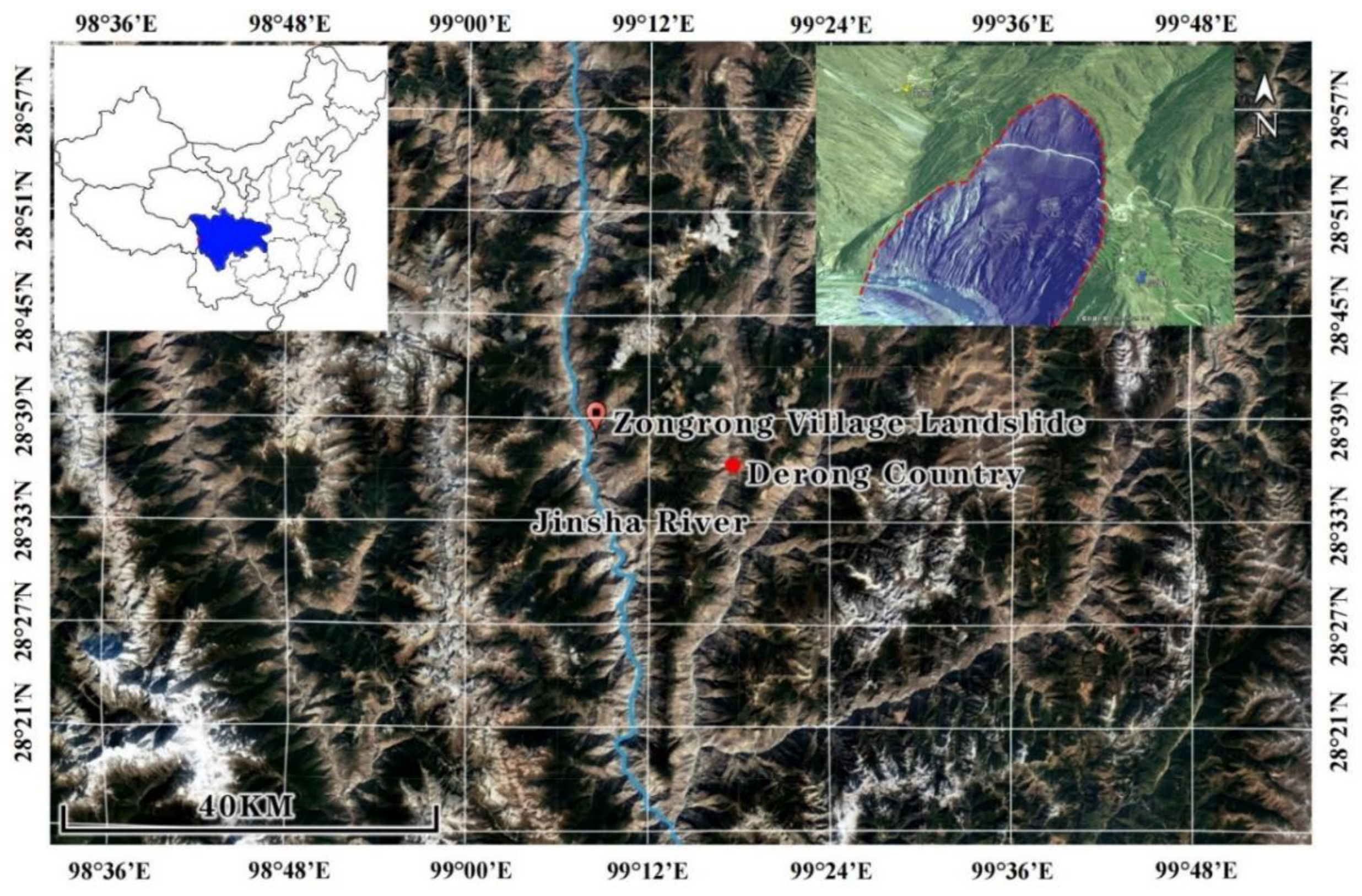
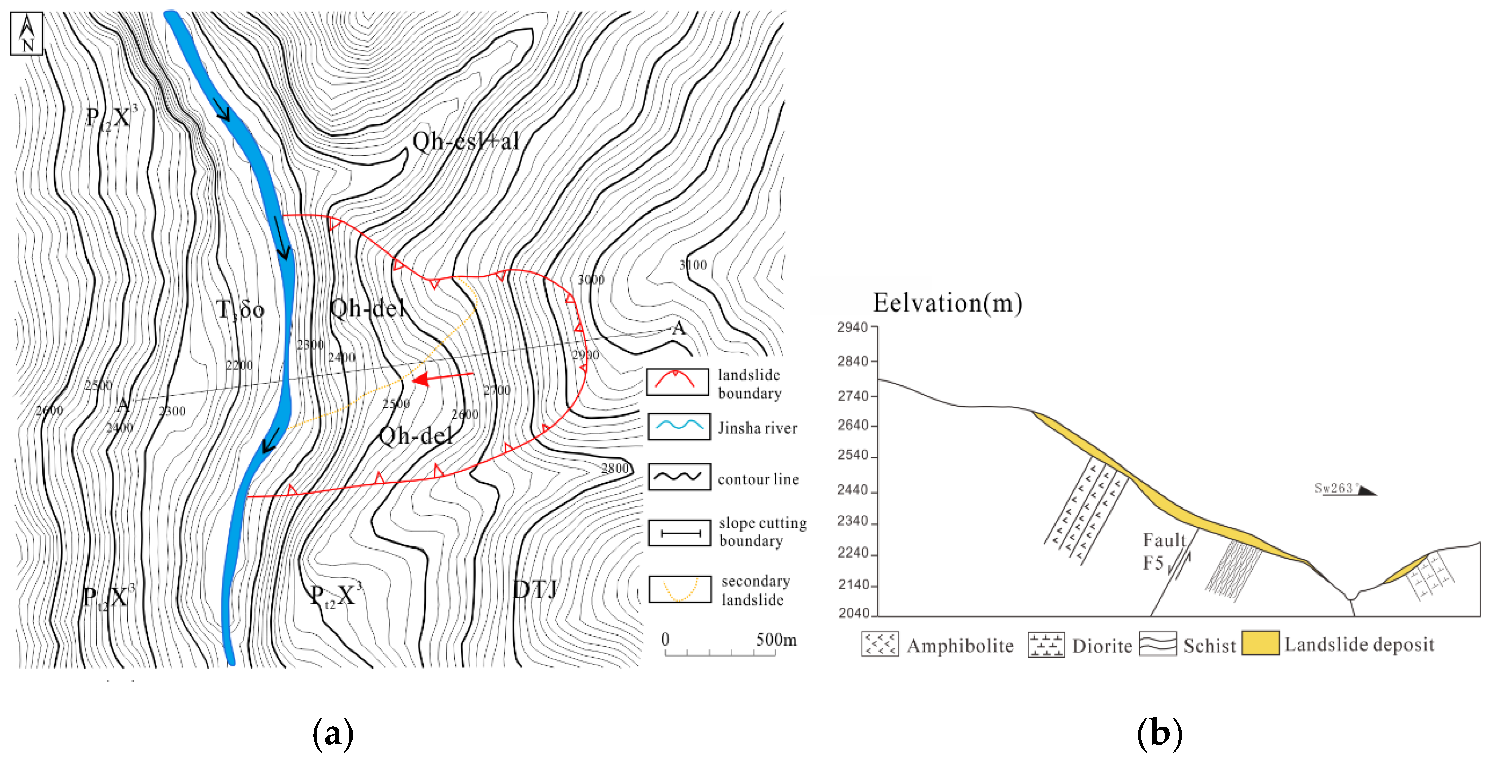
2. Geological Conditions of the Landslide Area
3. Shaking Table Test
3.1. Test Equipment
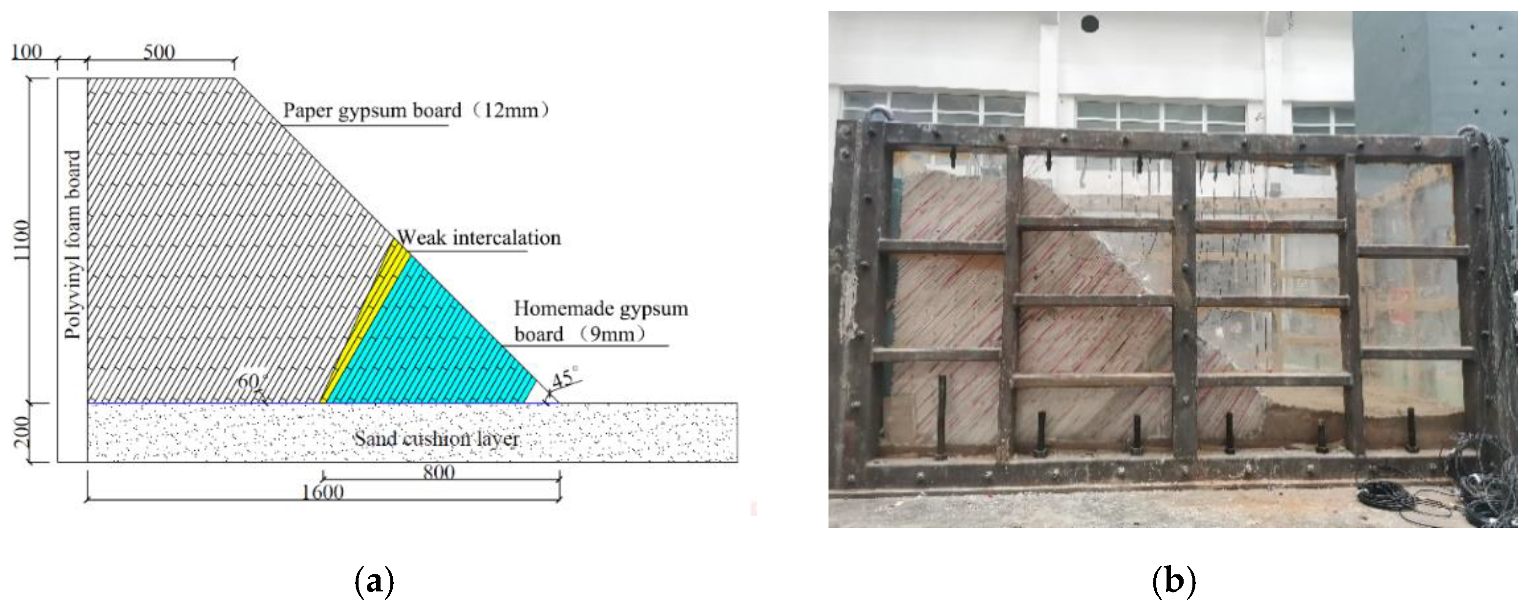
3.2. Physical Model Test
3.3. Material Used
3.4. Model Design
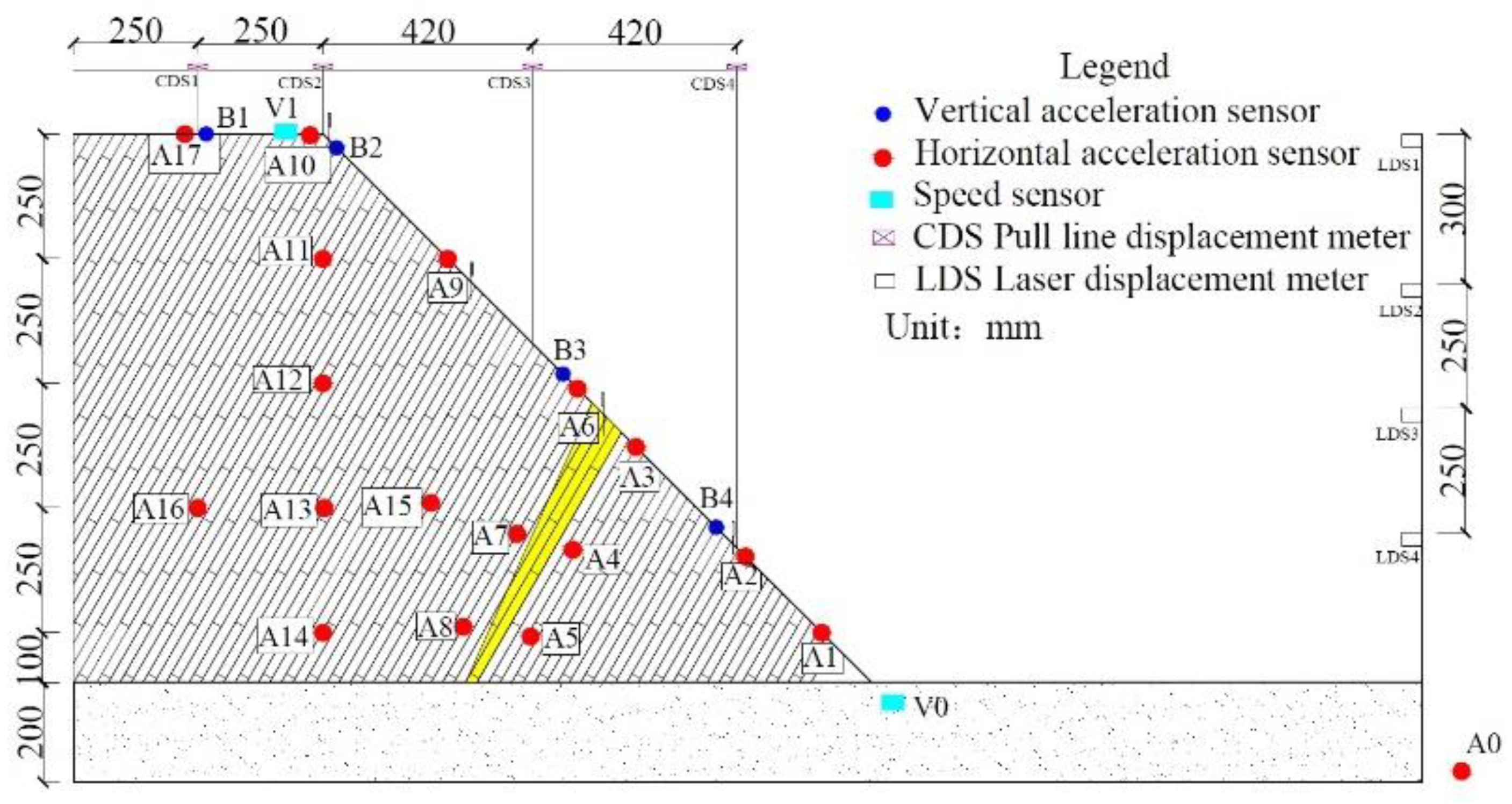
3.5. Monitoring Alternatives
3.6. Loading Scheme
4. Analysis of Slope Dynamic Characteristics
5. Analysis of Slope Dynamic Response Law and Influencing Factors
5.1. Basic Law of Slope
5.2. Influence of Dynamic Parameters
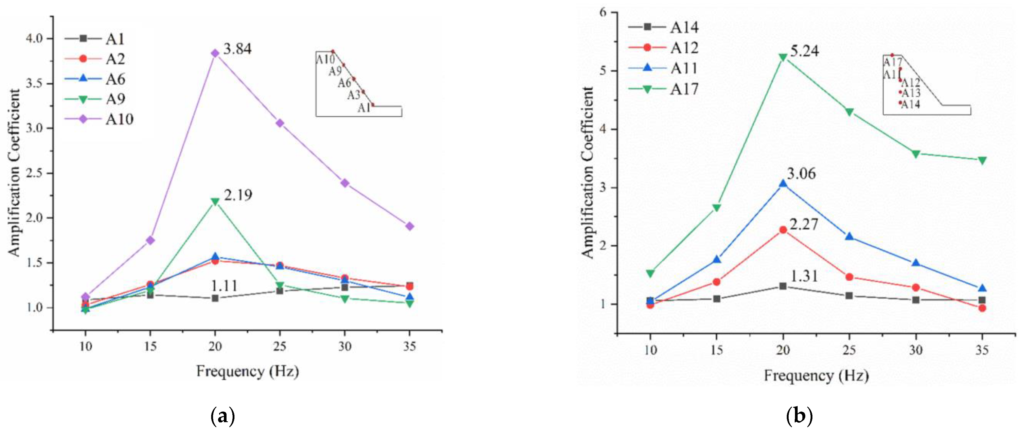
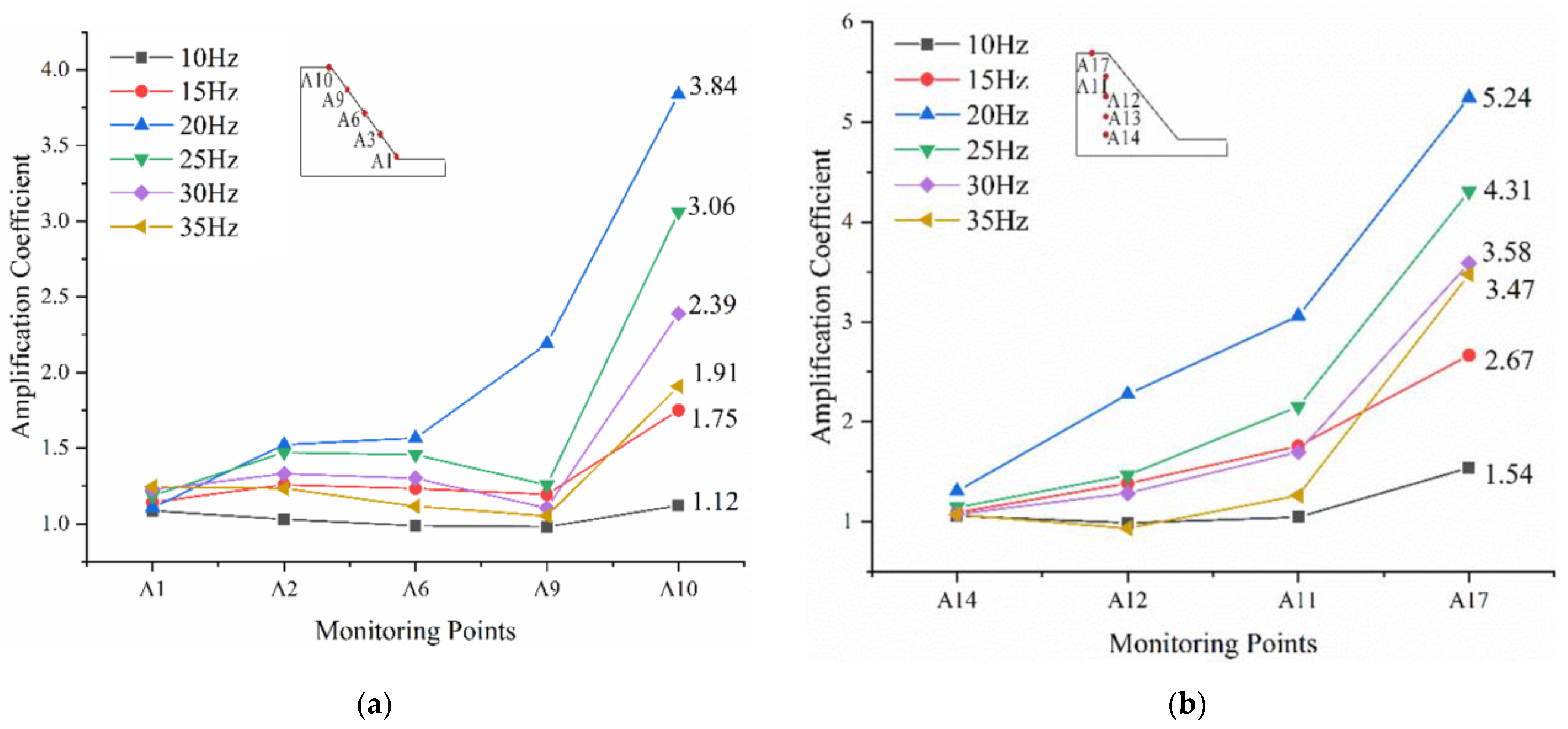
5.2.1. Influence of Frequency
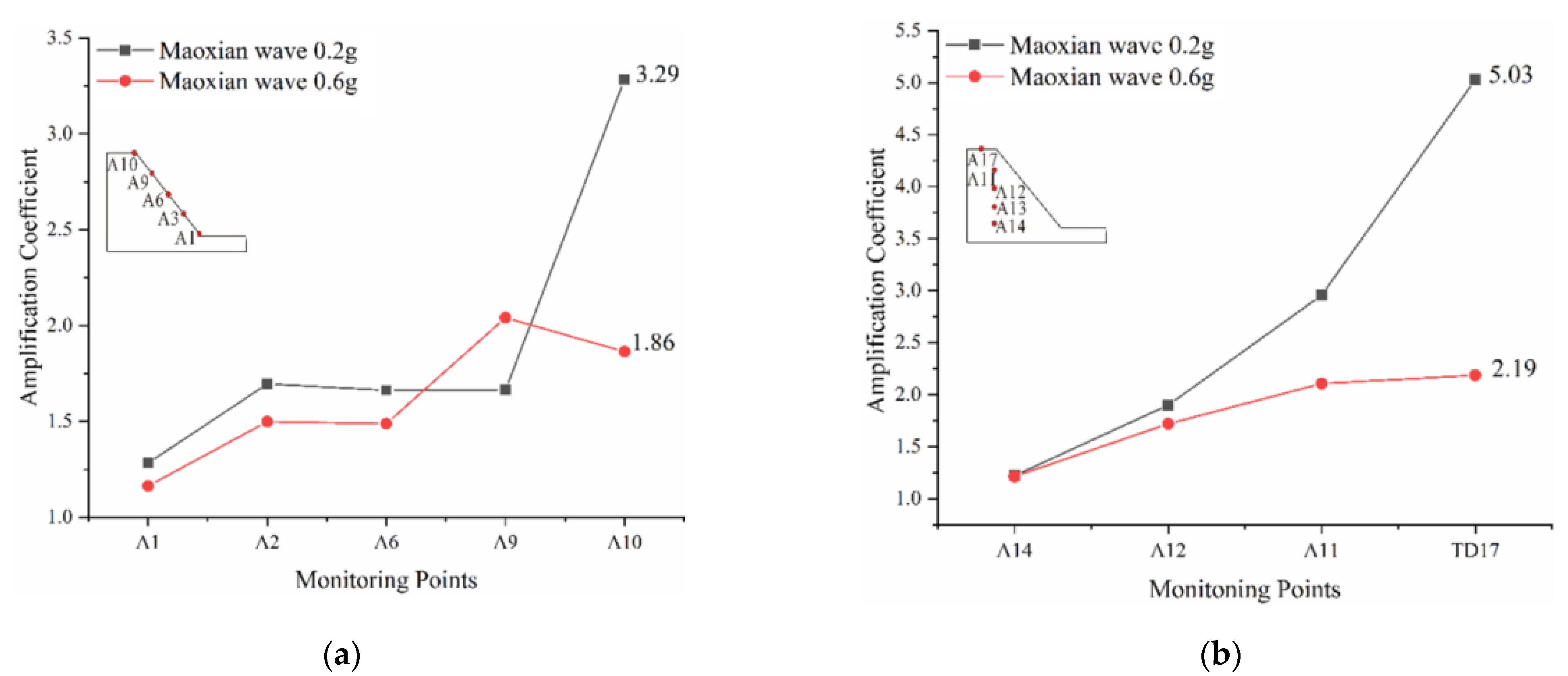
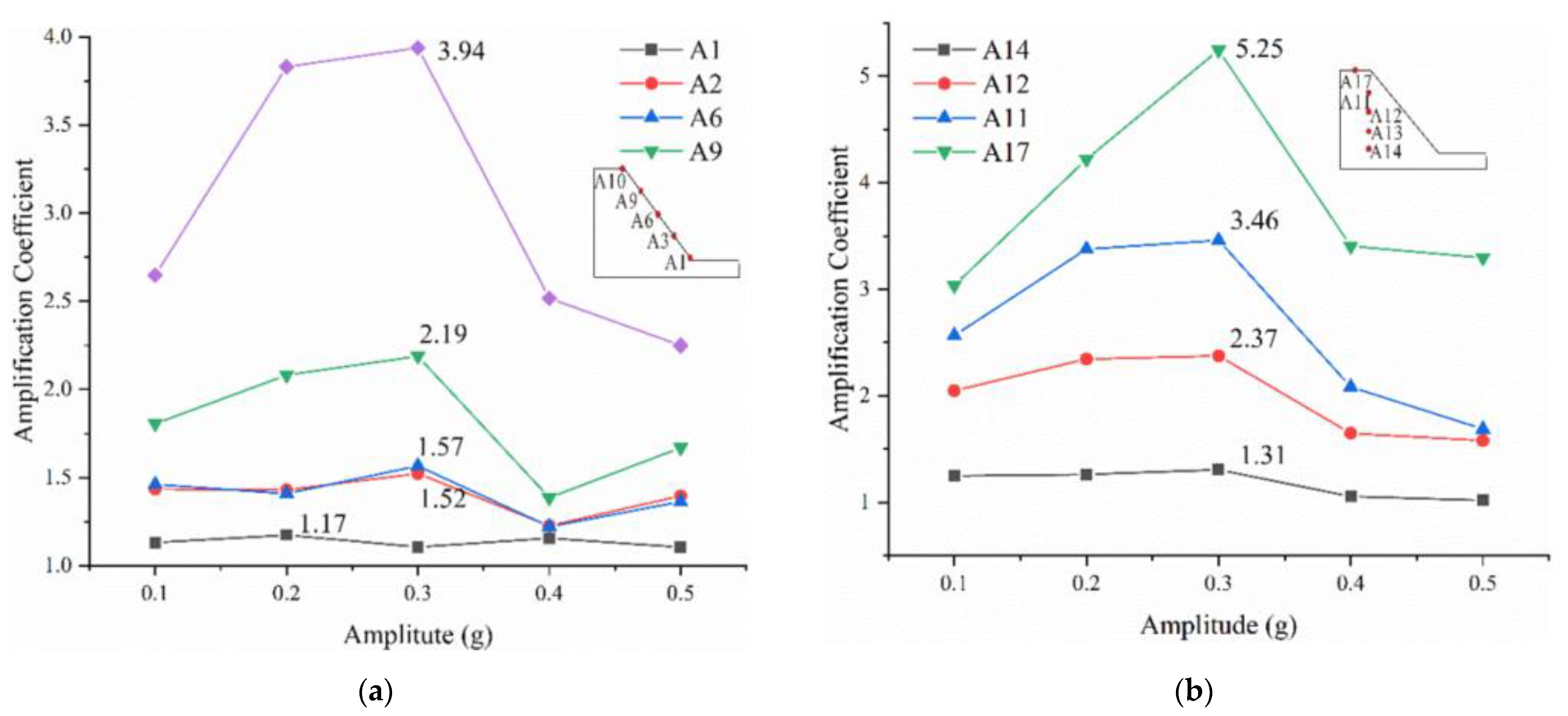
5.2.2. Influence of Amplitude
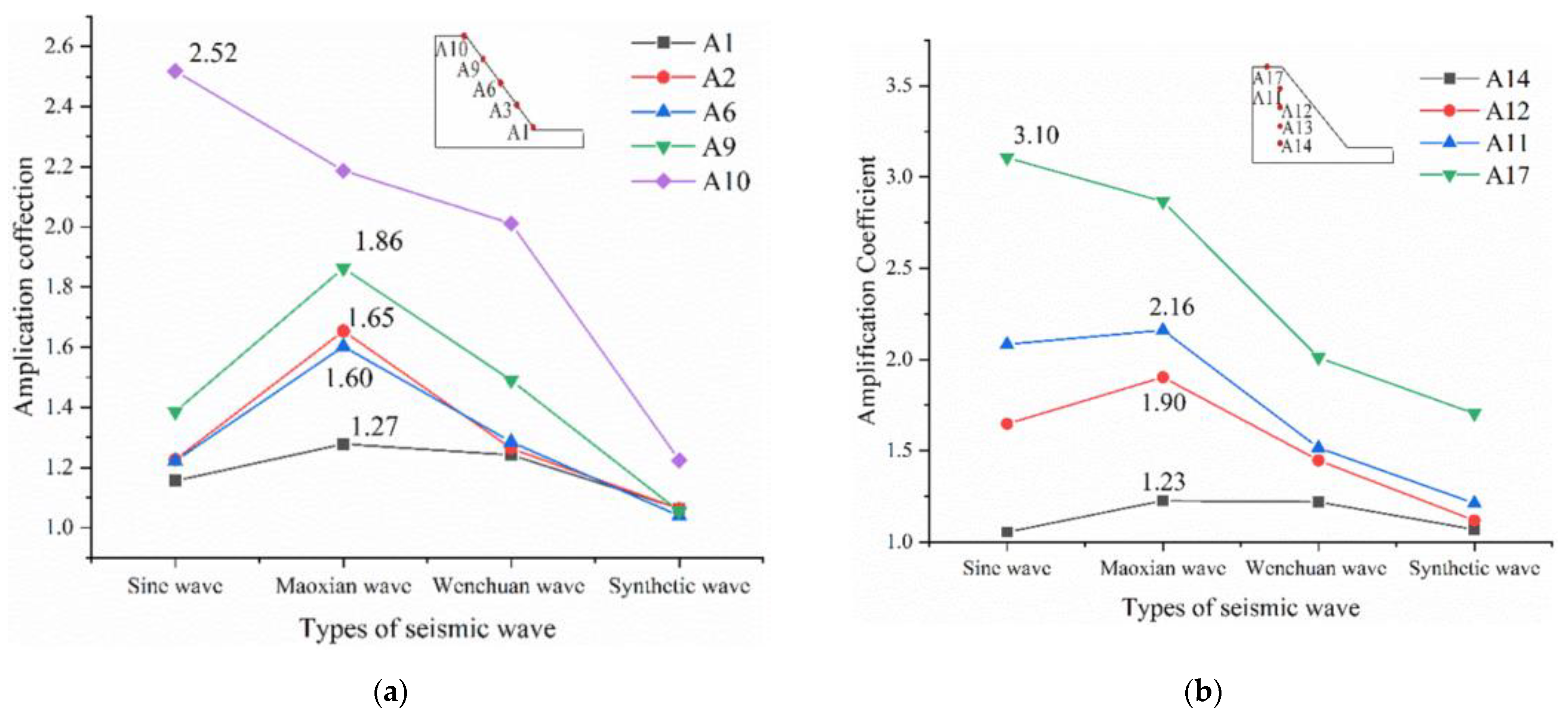
5.2.3. Influence of Seismic Wave Type
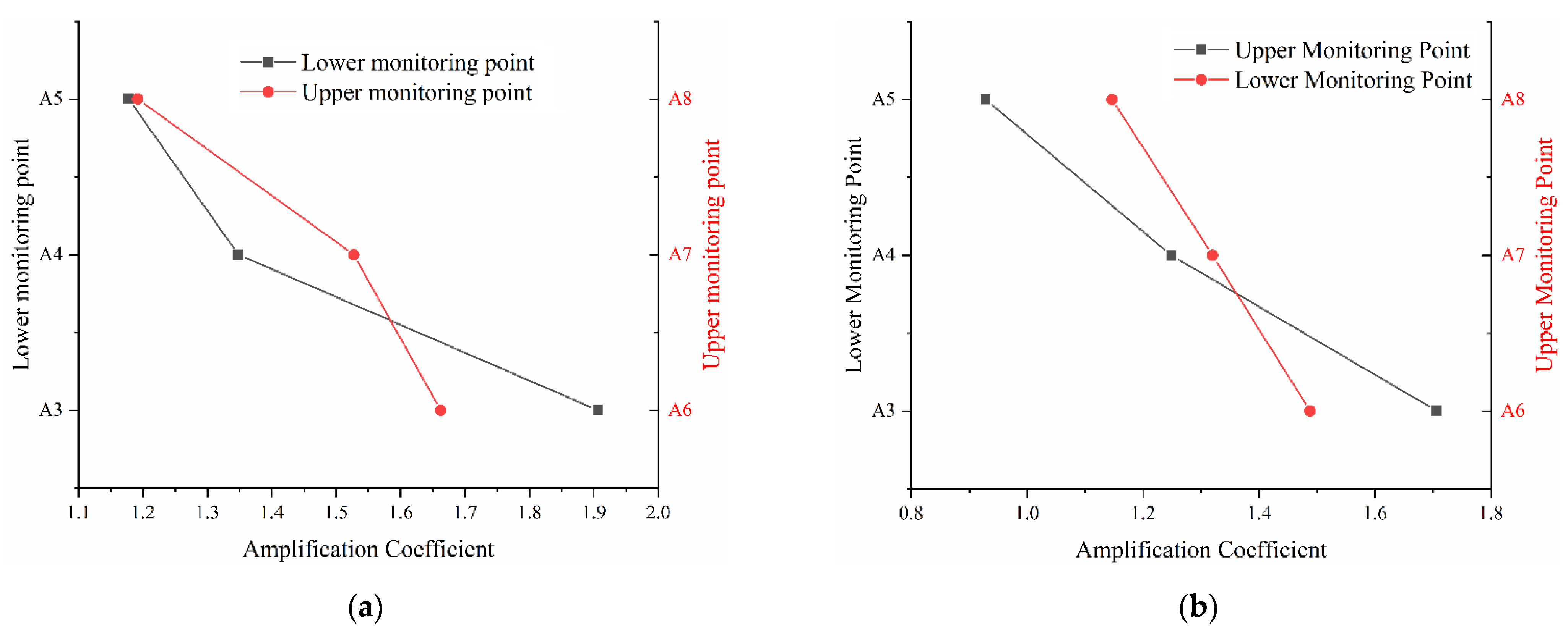
5.2.4. Influence of Structural Plane
6. Study on the Slope’s Failure Process
7. Conclusions
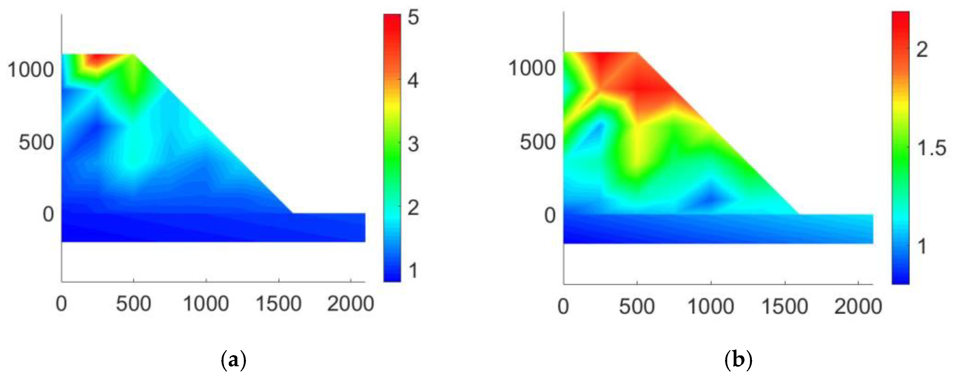
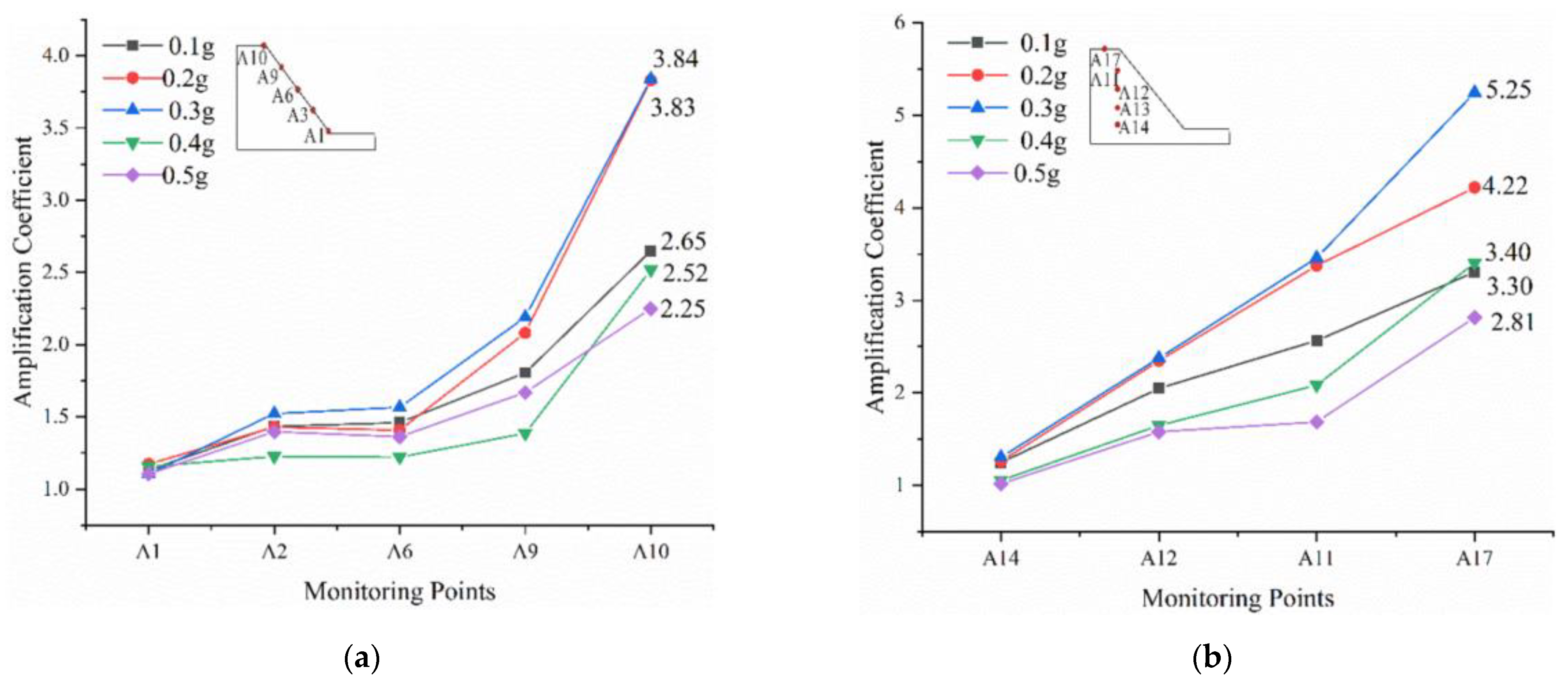
- The slope has an obvious “elevation effect” and “surface effect”, and the distribution range of the slope dynamic amplification effect is different under different amplitudes. The acceleration amplification factors of the slope surface and inside the slope show different increasing trends with elevation. The acceleration amplification factor of the inside slope increases linearly with an increase in elevation. However, the acceleration amplification factor of the slope surface increases slowly at first and then sharply with elevation, and the position of the obvious increase is controlled by the frequency and amplitude of the input wave. When the frequency of the input wave is close to the natural frequency of the slope or the amplitude is less than 0.3 g, the acceleration amplification factor of the slope surface increases sharply at the position of 1/2 the slope height, and increases sharply at the position of 3/4 of the slope height under the action of other input waves.
- The ground motion parameters have different effects on the slope’s dynamic response. The acceleration amplification factor of the slope first increases and then decreases with an increase in frequency, and the inflection point of the acceleration amplification factor is affected by the amplitude. When the input seismic wave frequency is near the natural frequency of the slope, the acceleration amplification factor of the slope increases first and then decreases with an increase in the input amplitude, and the amplitudes corresponding to the maximum acceleration amplification factors inside the slope and at the slope surface are different. Frequency affects the acceleration amplification growth rate of the slope, which is more obvious for the monitoring points inside the slope. The closer to the natural frequency of the slope, the faster the acceleration amplification factor curve increases. The amplitude has little effect on the rate of increase in the slope acceleration amplification factor.
- The amplification effect of the slope on different input waves was different. The amplification effect of the rocky slope on the input bedrock seismic waves is higher than that of the input soil seismic waves, but the amplification effect of the slope top on the sinusoidal waves is obviously higher than that of other types of input waves. Therefore, in shaking table tests, bedrock seismic waves should be used for rock slopes, and soil seismic waves should be used for soil slopes.
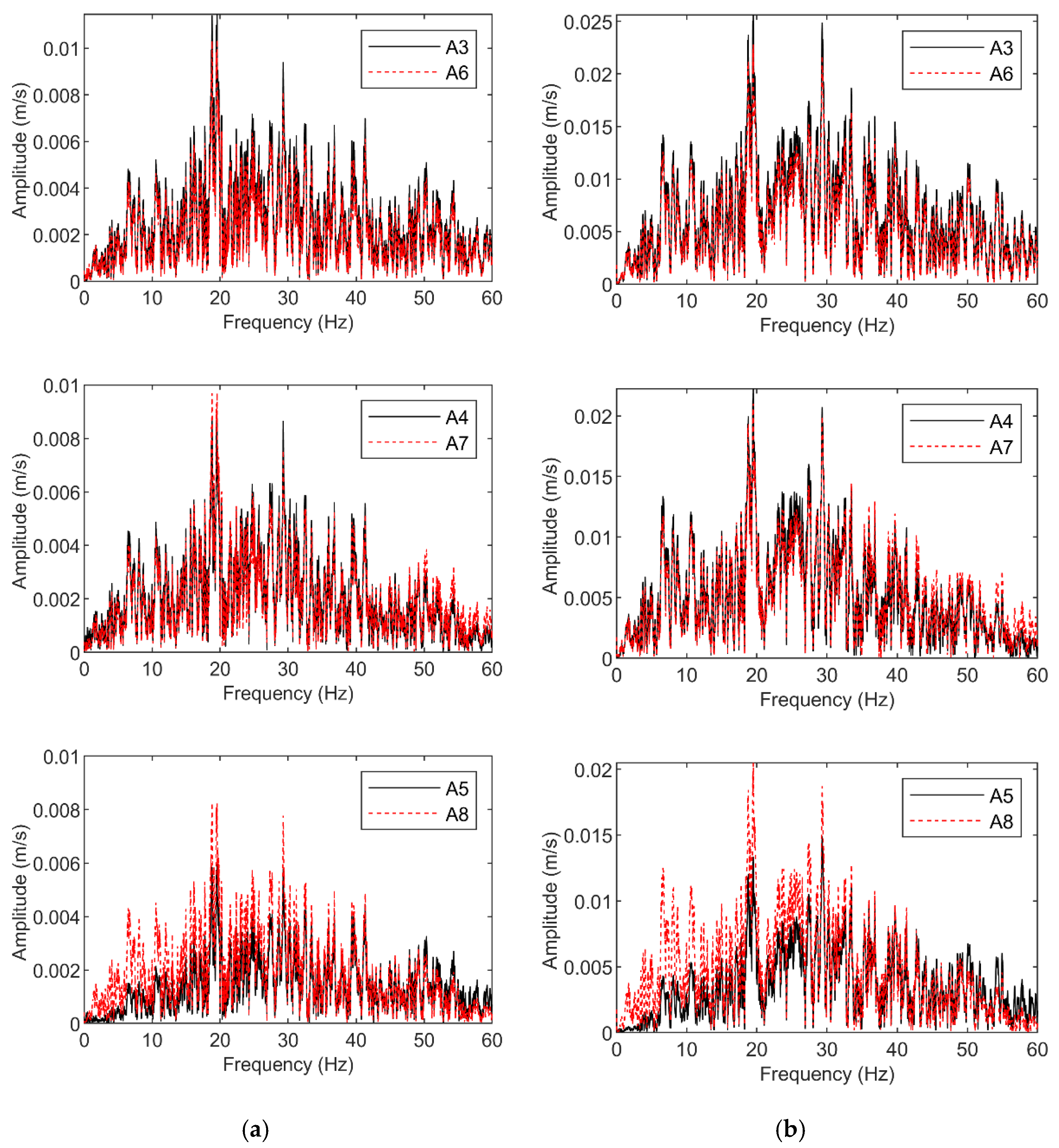
- The weak intercalated layer has no obvious effect on the change in the seismic wave spectrum; it shows good symmetry under different amplitudes. However, it can amplify or suppress the seismic wave energy, owing to the influence of the thickness of the soft structural plane. When the thickness of the weak section is low, the input seismic wave can be amplified. With an increase in the thickness of the soft structural plane, the amplification effect of the seismic wave is gradually weakened and even suppressed.
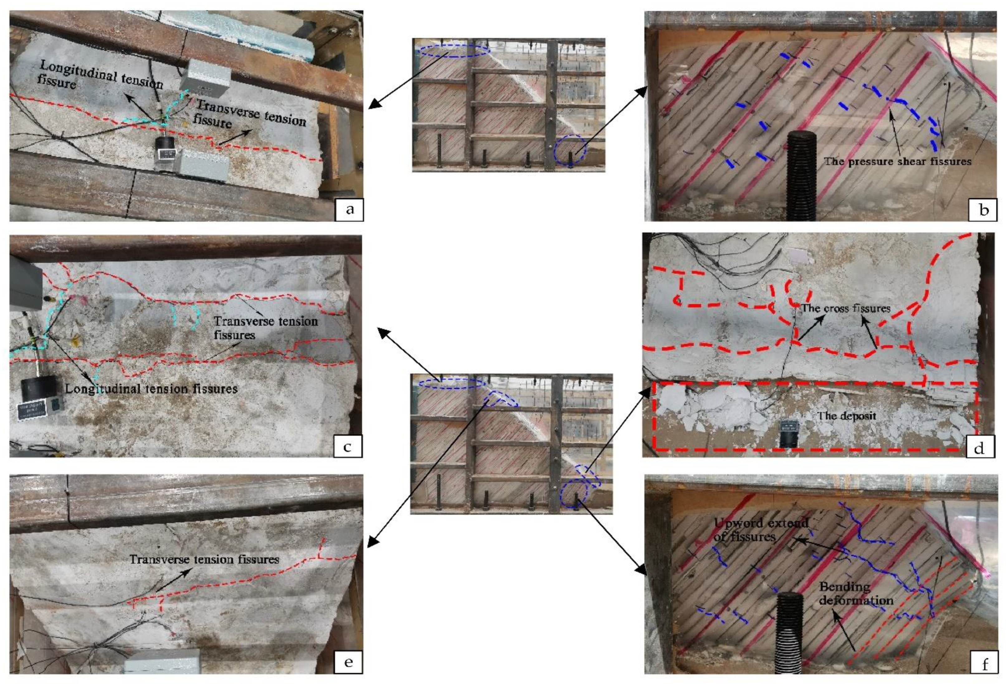
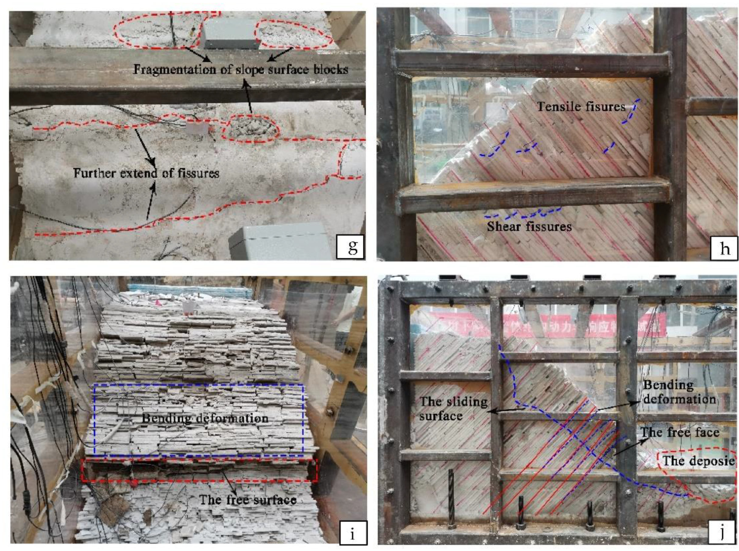
- The slope’s failure process can be roughly divided into three stages: (1) the formation of tensile cracks at the top and shear cracks at the toe; (2) the extension of cracks and the sliding of the slope-surface block; (3) the formation of the main sliding surface. The critical dynamic condition for slope fracture initiation is 0.3 g, and 0.8 g is the critical dynamic condition for slope failure.
Author Contributions
Funding
Institutional Review Board Statement
Informed Consent Statement
Data Availability Statement
Conflicts of Interest
References
- Dai, F.C.; Deng, J.H. Development characteristics of landslide hazards i n Three-rivers basin of Southeast Tibetan plateau. Adv. Eng. Sci. 2020, 52, 3–15. [Google Scholar]
- Li, S.; Chen, J.B.; Yao, Y.; Wu, G.D.; Xie, J.L. Risk analysis on seismic landslides by GIS: Take Yili area as an example. Inland Earthq. 2021, 35, 38–47. [Google Scholar]
- Yin, Y.P. Features of landslides triggered by the Wenchuan earthquake. J. Eng. Geol. 2009, 17, 29–38. [Google Scholar]
- Chigira, M.; Wu, X.Y.; Inokuc, T.; Wang, G.H. Landslides induced by the 2008 Wenchuan earthquake, Sichuan, China. Geomorphology 2010, 118, 225–238. [Google Scholar] [CrossRef]
- Li, G.; Hua, H.L.; Zhao, J.J. Spectrum characteristics of stratified rock slopes using shaking table test. J. Eng. Geol. 2016, 24, 959–966. [Google Scholar]
- Froude, M.J.; Petley, D.N. Global fatal landslide occurrence from 2004 to 2016. Nat. Hazards Earth Syst. Sci. 2018, 18, 2161–2181. [Google Scholar] [CrossRef] [Green Version]
- Chen, J.; Cui, Z.J. Discovery of outburst deposits induced by the Xuelongnang paleo landslide-dammed lake in the upper Jinsha river, China and its environmental and hazard significance. Acta Sedimentol. Sin. 2015, 33, 275–284. [Google Scholar]
- Huang, R.Q.; Pei, X.J.; Fan, X.M.; Zhang, W.F.; Li, S.G.; Li, B.L. The characteristics and failure mechanism of the largest landslide triggered by the Wenchuan earthquake, May 12, 2008, China. Landslides 2012, 1, 131–142. [Google Scholar] [CrossRef]
- Sepulveda, S.A.; Murphy, W.; Jibson, R.W.; Petley, D.N. Seismically induced rock slope failures resulting from topographic amplification of strong ground motions: The case of Pacoima Canyon, California. Eng. Geol. 2005, 80, 336–348. [Google Scholar] [CrossRef]
- Ma, N.; Wang, G.; Kamai, T.; Doi, I.; Chigira, M. Amplification of seismic response of a large deep-seated landslide in Tokushima, Japan. Eng. Geol. 2019, 249, 218–234. [Google Scholar] [CrossRef]
- Shen, T.; Wang, Y.S.; Luo, Y.H.; Xin, C.C.; Liu, Y. Seismic response of cracking features in Jubao Mountain during the aftershocks of Jiuzhaigou Ms7.0 earthquake. J. Mt. Sci. 2019, 16, 2532–2547. [Google Scholar] [CrossRef]
- Hu, X.L.; Wang, Y.S.; Liu, J.; Liu, Y.; Shen, T.; Xin, C.C. Analysis of ground motion response monitoring data of Xuejiaba site of Ms 4. 1 aftershock in Jiuzhaigou. Sci. Technol. Eng. 2019, 19, 49–55. [Google Scholar]
- Wang, Y.S.; He, J.X.; Luo, Y.H.; Hao, Z.H.; Liu, Y.; Zhang, L. Seismic responses of Lengzhuguan slope during Kangding Ms5.8 earthquake. J. Southwest Jiaotong Univ. 2015, 50, 838–844. [Google Scholar] [CrossRef]
- Wasowski, J.; Gaudio, V.D. Evaluating seismically induced mass movement hazard in Caramanico Terme (Italy). Eng. Geol. 2000, 58, 291–311. [Google Scholar] [CrossRef]
- Li, H.B.; Liu, Y.Q.; Liu, L.B.; Liu, B.; Xia, X. Numerical evaluation of topographic effects on seismic response of single-faced rock slopes. Bull. Eng. Geol. Environ. 2017, 78, 1873–1891. [Google Scholar] [CrossRef]
- He, J.X.; Qi, S.W.; Wang, Y.S.; Saroglou, C. Seismic response of the Lengzhuguan slope caused by topographic and geological effects. Eng. Geol. 2020, 265, 105431. [Google Scholar] [CrossRef]
- Wang, T.; Gao, C.L.; Huang, F.; Peng, D.; Tian, S.W.; Li, H.L. Dynamic response of rock slope with anti-dip weak intercalated layer and its influencing factors under seismic actions. Arab. J. Geosci. 2021, 14, 425. [Google Scholar] [CrossRef]
- Shi, G.X.; Guang, C.Z.; Jing, K.L. Laws of influence upon dynamic response of high rock slope by seismic wave frequency. Appl. Mech. Mater. 2012, 170, 615–625. [Google Scholar]
- Song, D.Q.; Che, A.L.; Zhu, R.J.; Ge, X.R. Natural frequency characteristics of rock masses containing a complex geological structure and their effects on the dynamic stability of slopes. Rock Mech. Rock Eng. 2019, 52, 4457–4473. [Google Scholar] [CrossRef]
- Song, D.Q.; Huang, J.; Liu, X.L. Dynamic response of layered rock slopes under earthquakes. J. Hunan Univ. (Nat. Sci. Ed.) 2021, 48, 113–120. [Google Scholar]
- Feng, X.X.; Jiang, Q.H.; Zhang, H.C.; Zhang, X.B. Study on the dynamic response of dip bedded rock slope using discontinuous deformation analysis (DDA) and shaking table tests. Int. J. Numer. Anal. Methods Geomech. 2020, 45, 411–427. [Google Scholar] [CrossRef]
- Mao, L.J.; Xu, Q.; Zheng, J.; Zhu, Y. Dynamic Responses of slope under the effect of seismic loads. Appl. Mech. Mater. 2013, 438, 1587–1591. [Google Scholar] [CrossRef]
- Zhao, L.Y.; Huang, Y.; Hu, H.Q. Stochastic seismic response of a slope based on large-scale shaking-table tests. Eng. Geol. 2020, 277, 105782. [Google Scholar] [CrossRef]
- Srilatha, N.; Madhavi Latha, G.; Puttappa, C.G. Effect of frequency on seismic response of reinforced soil slopes in shaking table tests. Geotext. Geomembr. 2013, 36, 27–32. [Google Scholar] [CrossRef]
- Feng, X.X.; Jiang, Q.H.; Zhang, X.B.; Zhang, H.C. Shaking table model test on the dynamic response of anti-dip rock slope. Geotech. Geol. Eng. 2019, 37, 1211–1221. [Google Scholar] [CrossRef]
- Zhou, Z.J.; Fan, Y.L.; Yan, K.F. Shaking table model test of slope seismic dynamic response. J. High. Transp. Res. Dev. Engl. Ed. 2017, 11, 23–32. [Google Scholar] [CrossRef]
- Liu, H.X.; Xu, Q.; Wang, L.; Hou, H.J. Effect of frequency of seismic wave on acceleration response of rock slopes. Chin. J. Rock Mech. Eng. 2014, 33, 125–133. [Google Scholar]
- Chen, C.C.; Li, H.H.; Chiu, Y.C.; Tsai, Y.K. Dynamic response of a physical anti-dip rock slope model revealed by shaking table tests. Eng. Geol. 2020, 277, 105772. [Google Scholar] [CrossRef]
- Liu, H.X.; Xu, Q.; Li, Y.R.; Fan, X.M. Response of high-strength rock slope to seismic waves in a shaking table test. Bull. Seismol. Soc. Am. 2013, 103, 3012–3025. [Google Scholar] [CrossRef]
- Yang, G.X.; Qi, S.W.; Wu, F.Q.; Zhan, Z.F. Seismic amplification of the anti-dip rock slope and deformation characteristics: A large-scale shaking table test. Soil Dyn. Earthq. Eng. 2018, 115, 907–916. [Google Scholar] [CrossRef]
- Chen, Z.L.; Hu, X.; Xu, Q. Experimental study of motion characteristics of rock slopes with weak intercalation under seismic excitation. J. Mt. Sci. 2016, 13, 546–556. [Google Scholar] [CrossRef]
- Li, H.H.; Lin, C.H.; Zu, W.; Chen, C.C.; Weng, M.C. Dynamic response of a dip slope with multi-slip planes revealed by shaking table tests. Landslides 2018, 15, 1731–1743. [Google Scholar] [CrossRef]
- He, J.X.; Qi, S.W.; Zhan, Z.F.; Guo, S.F.; Li, C.L.; Zheng, B.W.; Huang, X.L.; Zou, Y.; Yang, G.X.; Liang, N. Seismic response characteristics and deformation evolution of the bedding rock slope using a large-scale shaking table. Landslides 2021, 18, 2835–2853. [Google Scholar] [CrossRef]
- Li, M.L.; Wang, K.L. Seismic slope behavior in a large-scale shaking table model test. Eng. Geol. 2006, 86, 118–133. [Google Scholar]
- Fan, G.; Zhang, J.J.; Wu, J.B.; Yan, K.M. Dynamic Response and dynamic failure mode of a weak intercalated rock slope using a shaking table. Rock Mech. Rock Eng. 2016, 49, 3243–3256. [Google Scholar] [CrossRef]
- Li, L.Q.; Ju, N.P.; Zhang, S.X.; Deng, X.X. Shaking table test to assess seismic response differences between steep bedding and toppling rock slopes. Bull. Eng. Geol. Environ. 2019, 78, 519–531. [Google Scholar] [CrossRef]
- Deng, Z.Y.; Liu, X.R.; Liu, Y.Q.; Liu, S.L.; Han, Y.F.; Liu, J.H.; Tu, Y.L. Model test and numerical simulation on the dynamic stability of the bedding rock slope under frequent microseisms. Earthq. Eng. Eng. Vib. 2020, 19, 919–935. [Google Scholar] [CrossRef]
- Wang, K.L.; Lin, M.L. Initiation and displacement of landslide induced by earthquake—A study of shaking table model slope test. Eng. Geol. 2011, 122, 106–114. [Google Scholar] [CrossRef]
- Huang, D.; Ma, H.; Meng, Q.J.; Song, Y.X. Centrifugal model test and numerical simulation for anaclinal rock slopes with soft-hard interbedded structures. Chin. J. Geotech. Eng. 2020, 42, 1286–1295. [Google Scholar]
- Huang, D.; Xie, Z.Z.; Song, Y.X.; Meng, Q.J.; Luo, S.L. Centrifuge model test study on the toppling deformation of the anti-dip soft-hard interbedded rock slopes. Chin. J. Rock Mech. Eng. 2021, 40, 1357–1368. [Google Scholar]
- Li, Y.Q.; Huang, D.; Meng, Q.J. An analysis of the deformation characteristics of soft-hard interbedded anti-tilting layered rock slope based on centrifuge and numerical simulation. Hydrogeol. Eng. Geol. 2021, 48, 141–150. [Google Scholar]
- Li, S.J.; Sun, Q.C.; Zhang, Z.H.; Luo, X.Q. Physical modelling and numerical analysis of slope instability subjected to reservoir impoundment of the Three Gorges. Environ. Earth Sci. 2018, 77, 138–154. [Google Scholar] [CrossRef]
- Paster, M.; Martin Stickle, M.; Dutto, P.; Mira, P.; Fernández Merodo, J.A.; Blanc, T.; Sancho, S.; Benítez, A.S. A viscoplastic approach to the behaviour of fluidized geomaterials with application to fast landslides. Contin. Mech. Thermodyn. 2015, 27, 21–47. [Google Scholar] [CrossRef]
- Paster, M.; Blanc, T.; Haddad, B.; Petrone, S.; Sanchez Morles, M.; Drempetic, V.; Issler, D.; Crosta, G.B.; Cascini, L.; Sorbino, G.; et al. Application of a SPH depth-integrated model to landslide run-out analysis. Landslides 2014, 11, 793–812. [Google Scholar] [CrossRef] [Green Version]
- Kakogiannou, E.; Sanavia, L.; Nicot, F.; Darve, F.; Schrefler, B.A. A porous media finite element approach for soil instability including the second-order work criterion. Acta Geotech. 2016, 11, 805–825. [Google Scholar] [CrossRef]
- Sosio, R.; Giovanni, B.C.; Hungr, O. Complete dynamic modeling calibration for the Thurwieser rock avalanche (Italian Central Alps). Eng. Geol. 2008, 100, 11–26. [Google Scholar] [CrossRef]
- Xu, G.X.; Yao, L.K.; Gao, Z.N.; Li, Z.H. Large-scale shaking table model test study on dynamic characteristics and dynamic responses of slope. Chin. J. Rock Mech. Eng. 2008, 27, 624–632. [Google Scholar]
- Zhou, Z.P.; Huang, H.; Li, L.Q.; Huang, H.P.; Wei, H.B. Application study of transfer function in vibrating detection. Electron. Meas. Technol. 2018, 41, 126–130. [Google Scholar]
- Fan, G.; Zhang, J.J.; Fu, X.; Wang, M.Y. Application of transfer function to on-site shaking table test. Rock Soil Mech. 2016, 37, 2869–2876. [Google Scholar]
- Jiang, L.W.; Yao, L.K.; Wu, W.; Xu, G.X. Transfer function analysis of earthquake simulation shaking table model test of side slopes. Rock Soil Mech. 2010, 31, 1368–1374. [Google Scholar]


| Parameters | Definition | Reduced Scale |
|---|---|---|
| Length l | Cl | 100 * |
| Density ρ | Cγ | 1 * |
| Elastic modulus E | CE | 100 * |
| Cohesion φ | Cφ = CE | 100 |
| Friction angle c | Cc | 1 |
| Poisson’s ratio μ | Cμ | 1 |
| Acceleration a | Ca | 1 |
| Displacement d | Cd | 100 |
| Time t | Ct | 10 |
| Frequency f | Cf | 1/10 |
| Rock Types | Point-Load Strength/MPa | Compressive Strength Rc/MPa | Tensile Strength Rt/MPa | Cohesion/MPa | Friction Angle/° | Elastic Modulus/MPa | Poisson’s Ratio | Bulk Density/kN·m−2 |
|---|---|---|---|---|---|---|---|---|
| Ophiolite | 6.79 | 95.99 | 10.19 | 15.63 | 48.52 | 2384.0 | 0.19 | 28.60 |
| Diorite | 8.18 | 110.38 | 12.27 | 18.40 | 47.81 | 2537.2 | 0.19 | 25.35 |
| Gneiss | 6.15 | 89.12 | 9.23 | 13.34 | 38.90 | 1680.4 | 0.19 | 24.82 |
| Item | Density ρ/kN·m−2 | Elastic Modulus E/Mpa | Cohesion φ/Mpa | Friction Angle c | Poisson’s Ratio μ |
|---|---|---|---|---|---|
| Hardrock | 26.98 | 20.57 | 0.18 | 44.52 | 0.23 |
| Soft rock | 24.82 | 12.68 | 0.12 | 35.6 | 0.19 |
| Loading Sequence | Vibration Characteristics of Shaking Table |
|---|---|
| 1 | White noise (denoted as WN1) with an amplitude of 0.1 g |
| 2–7 | Sinusoidal wave is loaded in the sequence of excitation frequency 10–35 Hz and interval 5 Hz (hereinafter denoted as f = 10–35 Hz, Δf = 5 Hz) in the X direction of excitation with an amplitude of 0.1 g |
| 8–10 | Maoxian wave, Wenchuan wave, and 50-year exceedance probability are 10% (hereinafter denoted as 50–10%), and the amplitude is 0.1 g |
| 11 | White noise (denoted as WN2) with an amplitude of 0.1 g |
| 12–17 | Sinusoidal wave (f = 10~35 Hz, Δf = 5 Hz), X-direction excitation; the amplitude is 0.2 g |
| 18–21 | Maoxian wave, Wenchuan wave, 100–10%, 50–2%; the amplitude is 0.2 g |
| 22 | White noise (denoted as WN3) with an amplitude of 0.1 g |
| 23–28 | Sinusoidal wave (f = 10~35 Hz, Δf = 5 Hz), X-direction excitation; the amplitude is 0.3 g |
| 29–31 | Maoxian wave, Wenchuan wave, 100–2%; the amplitude is 0.3 g and 0.281 g, respectively |
| 32 | White noise (denoted as WN4) with an amplitude of 0.1 g |
| 33–38 | Sinusoidal wave (f = 10~35 Hz, Δf = 5 Hz), X-direction excitation; the amplitude is 0.4 g |
| 39–41 | Maoxian wave, Wenchuan wave, 100–0.1%; the amplitude is 0.4 g |
| 42 | White noise (denoted as WN5) with an amplitude of 0.1 g |
| 43–46 | Sinusoidal wave (f = 10~25 Hz, Δf = 5 Hz), X-direction excitation; the amplitude is 0.5 g |
| 47–49 | Maoxian wave, Wenchuan wave; the amplitude is 0.5 g; white noise (denoted as WN6) with an amplitude of 0.1 g |
| 50–52 | Maoxian wave, Wenchuan wave; the amplitude is 0.6 g; white noise (denoted as WN7) with an amplitude of 0.1 g |
| 53–55 | Maoxian wave, Wenchuan wave; the amplitude is 0.7 g; white noise (denoted as WN8) with an amplitude of 0.1 g |
| 56–58 | Maoxian wave, Wenchuan wave; the amplitude is 0.8 g; white noise (denoted as WN9) with an amplitude of 0.1 g |
| 59–61 | Maoxian wave, Wenchuan wave; the amplitude is 0.9 g; white noise (denoted as WN10) with an amplitude of 0.1 g |
| 62–64 | Maoxian wave, Wenchuan wave; the amplitude is 1.0 g; white noise (denoted as WN11) with an amplitude of 0.1 g |
Publisher’s Note: MDPI stays neutral with regard to jurisdictional claims in published maps and institutional affiliations. |
© 2022 by the authors. Licensee MDPI, Basel, Switzerland. This article is an open access article distributed under the terms and conditions of the Creative Commons Attribution (CC BY) license (https://creativecommons.org/licenses/by/4.0/).
Share and Cite
Guo, M.-Z.; Gu, K.-S.; Wang, C. Dynamic Response and Failure Process of a Counter-Bedding Rock Slope under Strong Earthquake Conditions. Symmetry 2022, 14, 103. https://doi.org/10.3390/sym14010103
Guo M-Z, Gu K-S, Wang C. Dynamic Response and Failure Process of a Counter-Bedding Rock Slope under Strong Earthquake Conditions. Symmetry. 2022; 14(1):103. https://doi.org/10.3390/sym14010103
Chicago/Turabian StyleGuo, Ming-Zhu, Kun-Sheng Gu, and Chen Wang. 2022. "Dynamic Response and Failure Process of a Counter-Bedding Rock Slope under Strong Earthquake Conditions" Symmetry 14, no. 1: 103. https://doi.org/10.3390/sym14010103