Lie Symmetry Analysis, Conservation Laws, Power Series Solutions, and Convergence Analysis of Time Fractional Generalized Drinfeld-Sokolov Systems

Abstract

In this work, we investigate invariance analysis, conservation laws, and exact power series solutions of time fractional generalized Drinfeld–Sokolov systems (GDSS) using Lie group analysis. Using Lie point symmetries and the Erdelyi–Kober (EK) fractional differential operator, the time fractional GDSS equation is reduced to a nonlinear ordinary differential equation (ODE) of fractional order. Moreover, we have constructed conservation laws for time fractional GDSS and obtained explicit power series solutions of the reduced nonlinear ODEs that converge. Lastly, some figures are presented for explicit solutions.

1. Introduction

Because of the great importance of nonlinear fractional partial differential equations (NFPDEs) in physics, mechanics, hydrology, viscoelasticity, image processing, electromagnetics, and other fields, researchers have long been aware of the solutions and applications of fractional partial differential equations [1,2,3,4,5,6,7,8,9,10,11,12]. In recent years, parallel to the increase in mathematical techniques and the use of computer programs, many authors have an increased desire to work on fractional analysis. Therefore, many methods are used to solve the NFPDEs—for example, the finite-difference method [13], the multiple exp-function method [14], the homotopy perturbation method [15,16], the variational-iteration method, the exp method [17], the fractional sub-equation method [18], and the Lie invariance method [19,20,21]. When we look through the literature, we realize Sophus Lie firstly put forward a methodology about symmetry analysis at the end of the nineteenth century [22]. After that, some impressive Lie group methods were considered in order to obtain symmetries, symmetry groups, and symmetry reduction. These are the classical and nonclasical Lie group approaches [23,24] and the Clarkson and Kruksal direct methods [25,26]. The main role of Lie symmetry methods is to construct invariance properties having partial equations as invariant forms. With the aid of these properties, we can reduce an NFPDE into a nonlinear ODE of fractional order with the help of the Riemann-Liouville (RL) derivative.

The link between Lie symmetry analysis and conservation laws of differential equations was revealed by Noether [27]. A generalized Noether theorem was used in [28] to construct conservation laws of NFPDEs with fractional Lagrangians. However, some differential equations do not arise from Lagrangians. To overcome this problem, İbragimov [29] put forward a new method without Lagrangians. Lukashchuk [30] showed important results towards obtaining conservation laws of NFPDEs.

In this study, we deal with exact solutions of the time fractional GDSS by using Lie symmetry analysis and conservation laws. The time fractional GDSS that models 1D nonlinear wave processes in two-component media has the form

$$\begin{array}{cc}\hfill & D_t^{\alpha }u+a_{1}u{u}_x+b_1{u}_{xxx}+c{\left(v^q\right)}_x=0,\hfill \\ \hfill & D_t^{\alpha }v+a_{2}u{v}_x+b_2{v}_{xxx}=0,\hfill \end{array}$$

(1)

where $a_1$, $a_2$, $b_1$, $b_2$, c, and q are arbitrary constants, and $D_t^{\alpha }$ is the RL fractional derivative defined in (2). We could not take $b_1$ = $b_2$ = 0, because the time fractional GDSS may develop finite time singularities [31,32,33]. According to our research, Lie symmetry methods have not been applied to the time fractional GDSS until now. With some special choices of $a_1$, $a_2$, $b_1$, $b_2$, c, and q, the equation can be reduced to the time fractional Drinfeld-Sokolov-Satsuma-Hirota equations discussed in [34].

The RL fractional partial derivative [35] is defined by

$$D_t^{\alpha }u=\left\{\begin{array}{cc}\frac{{\partial }^{m}u}{{\partial }^t},\hfill & \alpha =m\in N,\hfill \\ \frac{1}{\Gamma (m-\alpha )}\frac{{\partial }^m}{\partial t^m}{\int }_0^t\frac{u(z,x)}{{(t-z)}^{(\alpha +1-m)}}dz,\hfill & m-1<\alpha <m,m\in N,\hfill \end{array}\right.$$

(2)

where $\Gamma \left(z\right)$ is a Gamma function defined by

$$\Gamma \left(z\right)={\int }_0^{\infty }{e}^{-t}{t}^{z-1}dt,$$

which converges in the complex plane when $Re\left(z\right)>0$.

2. Preliminaries for Symmetry Analysis

In this chapter, we give the basic idea of the Lie symmetry method. Consider a system of time fractional partial differential equations with independent variables x and t as follows:

$$D_t^{\alpha }u(x,t)=F_1\left(x,t,u,u_t,u_x,u_{xx},v,v_t,v_x,v_{xx,\dots }\right),$$

(3)

$$D_t^{\alpha }v(x,t)=F_2\left(x,t,u,u_t,u_x,u_{xx},v,v_t,v_x,v_{xx,\dots }\right),$$

(4)

where the subscripts denote partial derivatives. Equations (3) and (4) are invariant under a one-parameter Lie group of point transformations given as follows:

$$\begin{array}{cc}\hfill & \overline{t}=t+ϵ\tau (t,x,u,v)+O\left({ϵ}^2\right),\overline{x}=x+ϵ\zeta (t,x,u,v)+O\left({ϵ}^2\right),\hfill \\ \hfill & \overline{u}=u+ϵ\mu (t,x,u,v)+O\left({ϵ}^2\right),\overline{v}=v+ϵ\rho (t,x,u,v)+O\left({ϵ}^2\right),\hfill \\ \hfill & \frac{{\partial }^{\alpha }\overline{u}}{\partial {\overline{t}}^{\alpha }}=\frac{{\partial }^{\alpha }u}{\partial t^{\alpha }}+ϵ{\mu }_{\alpha }^0(t,x,u,v)+O\left({ϵ}^2\right),\frac{{\partial }^{\alpha }\overline{v}}{\partial {\overline{t}}^{\alpha }}=\frac{{\partial }^{\alpha }v}{\partial t^{\alpha }}+ϵ{\rho }_{\alpha }^0(t,x,u,v)+O\left({ϵ}^2\right),\hfill \\ \hfill & \frac{\partial \overline{u}}{\partial \overline{x}}=\frac{\partial u}{\partial x}+ϵ{\mu }^x(t,x,u,v)+O\left({ϵ}^2\right),\frac{{\partial }^2\overline{u}}{\partial {\overline{x}}^2}=\frac{{\partial }^{2}u}{\partial x^2}+ϵ{\mu }^{xx}(t,x,u,v)+O\left({ϵ}^2\right),\hfill \\ \hfill & \frac{{\partial }^3\overline{u}}{\partial {\overline{x}}^3}=\frac{{\partial }^{3}u}{\partial x^3}+ϵ{\mu }^{xxx}(t,x,u,v)+O\left({ϵ}^2\right),\frac{\partial \overline{v}}{\partial \overline{x}}=\frac{\partial v}{\partial x}+ϵ{\rho }^x(t,x,u,v)+O\left({ϵ}^2\right),\hfill \\ \hfill & \frac{{\partial }^2\overline{v}}{\partial \overline{x^2}}=\frac{{\partial }^{2}v}{\partial x^2}+ϵ{\rho }^{xx}(t,x,u,v)+O\left({ϵ}^2\right),\frac{{\partial }^3\overline{v}}{\partial {\overline{x}}^3}=\frac{{\partial }^{3}v}{\partial x^3}+ϵ{\rho }^{xxx}(t,x,u,v)+O\left({ϵ}^2\right),\hfill \end{array}$$

(5)

where

$$\begin{array}{cc}\hfill & {\mu }^x=D_x\left(\mu \right)-u_x{D}_x\left(\zeta \right)-u_t{D}_x\left(\tau \right),\hfill \\ \hfill & {\mu }^{xx}=D_x\left({\mu }^x\right)-u_{xx}{D}_x\left(\zeta \right)-u_{xt}{D}_x\left(\tau \right),\hfill \\ \hfill & {\mu }^{xxx}=D_x\left({\mu }^{xx}\right)-u_{xxx}{D}_x\left(\zeta \right)-u_{xxt}{D}_x\left(\tau \right),\hfill \\ \hfill & {\rho }^x=D_x\left(\rho \right)-v_x{D}_x\left(\zeta \right)-v_t{D}_x\left(\tau \right),\hfill \\ \hfill & {\rho }^{xx}=D_x\left({\rho }^x\right)-v_{xx}{D}_x\left(\zeta \right)-v_{xt}{D}_x\left(\tau \right),\hfill \\ \hfill & {\rho }^{xxx}=D_x\left({\rho }^{xx}\right)-v_{xxx}{D}_x\left(\zeta \right)-v_{xxt}{D}_x\left(\tau \right),\hfill \\ \hfill & {\mu }_{\alpha }^0=D_t^{\alpha }\left(\mu \right)+\zeta D_t^{\alpha }\left(u_x\right)-D_t^{\alpha }\left(\zeta u_x\right)+D_t^{\alpha }\left(u\left(D_t\rho \right)\right)-D_t^{\alpha +1}\left(\rho u\right)+\rho D_t^{\alpha +1}\left(u\right),\hfill \\ \hfill & {\rho }_{\alpha }^0=D_t^{\alpha }\left(\rho \right)+\zeta D_t^{\alpha }\left(v_x\right)-D_t^{\alpha }\left(\zeta v_x\right)+D_t^{\alpha }\left(v\left(D_t\rho \right)\right)-D_t^{\alpha +1}\left(\rho v\right)+\rho D_t^{\alpha +1}\left(v\right),\hfill \end{array}$$

(6)

wherein $D_x$ and $D_t$ are total differential operators given as follows:

$$\begin{array}{cc}\hfill & D_x=\frac{\partial }{\partial x}+u_x\frac{\partial }{\partial u}+u_{xx}\frac{\partial }{\partial u_x}+v_x\frac{\partial }{\partial v}+v_{xx}\frac{\partial }{\partial v_x}+\dots ,\hfill \\ \hfill & D_t=\frac{\partial }{\partial t}+u_t\frac{\partial }{\partial u}+u_{tt}\frac{\partial }{\partial u_t}+v_t\frac{\partial }{\partial v}+v_{tt}\frac{\partial }{\partial v_t}+\dots .\hfill \end{array}$$

(7)

The infinitesimal generator of Equations (3) and (4) consists of a set of vector fields given by

$$X=\zeta \frac{\partial }{\partial x}+\tau \frac{\partial }{\partial t}+\mu \frac{\partial }{\partial u}+\rho \frac{\partial }{\partial v}.$$

(8)

One can prove that the infinitesimal generators defined above must satisfy the following invariance criterion for Equations (3) and (4):

$$P{r}^{n}X\left({\Delta }_1\right){{|}_{{\Delta }_1=0}=0andP{r}^{n}X\left({\Delta }_2\right)|}_{{\Delta }_2=0}=0,n=1,2,..,$$

(9)

where

$${\Delta }_1:=D_t^{\alpha }u(x,t)-F_1\left(x,t,u,u_t,u_x,u_{xx},v,v_t,v_x,v_{xx,\dots }\right),$$

and

$${\Delta }_2:=D_t^{\alpha }v(x,t)-F_2\left(x,t,u,u_t,u_x,u_{xx},v,v_t,v_x,v_{xx,\dots }\right).$$

As the lower limit of integral in (1) is fixed, it is going to be invariant under the transformations given in (5), so the corresponding invariance condition becomes

$$\tau (t,x,u,v)=0.$$

(10)

Under the condition (9), the $\alpha$-th infinitesimal related to RL fractional time derivative [36] is given by

$$\begin{array}{cc}\hfill & {\mu }_{\alpha }^0=\frac{{\partial }^{\alpha }\mu }{\partial t^{\alpha }}+\left({\mu }_u-\alpha D_t\left(\tau \right)\right)\frac{{\partial }^{\alpha }u}{\partial t^{\alpha }}-u\frac{{\partial }^{\alpha }{\mu }_u}{\partial t^{\alpha }}-v\frac{{\partial }^{\alpha }{\mu }_v}{\partial t^{\alpha }}+{\mu }_v\frac{{\partial }^{\alpha }v}{\partial t^{\alpha }}-\sum _{n=1}^{\infty }\left(\genfrac{}{}{0pt}{}{\alpha }{n}\right)D_t^n\left(\zeta \right)D_t^{\alpha -n}\left(u_x\right)\hfill \\ \hfill & +\sum _{n=1}^{\infty }\left[\left(\genfrac{}{}{0pt}{}{\alpha }{n}\right)\frac{{\partial }^n{\mu }_u}{\partial t^n}-\left(\genfrac{}{}{0pt}{}{\alpha }{n+1}\right)D_t^{n+1}\left(\tau \right)\right]D_t^{\alpha -n}\left(u\right)+\sum _{n=1}^{\infty }\left(\genfrac{}{}{0pt}{}{\alpha }{n}\right)\frac{{\partial }^n{\mu }_v}{\partial t^n}{D}_t^{\alpha -n}\left(v\right)+\lambda ,\hfill \\ \\ \hfill & {\rho }_{\alpha }^0=\frac{{\partial }^{\alpha }\rho }{\partial t^{\alpha }}+\left({\rho }_v-\alpha D_t\left(\tau \right)\right)\frac{{\partial }^{\alpha }v}{\partial t^{\alpha }}-u\frac{{\partial }^{\alpha }{\rho }_u}{\partial t^{\alpha }}-v\frac{{\partial }^{\alpha }{\rho }_v}{\partial t^{\alpha }}+{\rho }_u\frac{{\partial }^{\alpha }u}{\partial t^{\alpha }}-\sum _{n=1}^{\infty }\left(\genfrac{}{}{0pt}{}{\alpha }{n}\right)D_t^n\left(\zeta \right)D_t^{\alpha -n}\left(v_x\right)\hfill \\ \hfill & +\sum _{n=1}^{\infty }\left[\left(\genfrac{}{}{0pt}{}{\alpha }{n}\right)\frac{{\partial }^n{\rho }_v}{\partial t^n}-\left(\genfrac{}{}{0pt}{}{\alpha }{n+1}\right)D_t^{n+1}\left(\tau \right)\right]D_t^{\alpha -n}\left(v\right)+\sum _{n=1}^{\infty }\left(\genfrac{}{}{0pt}{}{\alpha }{n}\right)\frac{{\partial }^n{\rho }_u}{\partial t^n}{D}_t^{\alpha -n}\left(u\right)+\beta ,\hfill \end{array}$$

where

$$\begin{array}{cc}\hfill & \lambda =\sum _{n=2}^{\infty }\sum _{m_1+m_2=2}^n\sum _{k_1=0}^{m_1}\sum _{r_1=0}^{k_1}\sum _{k_2=0}^{m_2}\sum _{r_2=0}^{k_2}\left(\genfrac{}{}{0pt}{}{\alpha }{n}\right)\left(\genfrac{}{}{0pt}{}{n}{m_1}\right)\left(\genfrac{}{}{0pt}{}{n-m_1}{m_2}\right)\left(\genfrac{}{}{0pt}{}{k_1}{r_1}\right)\left(\genfrac{}{}{0pt}{}{k_2}{r_2}\right)\frac{1}{k_1!k_2!}\frac{t^{n-\alpha }}{\Gamma (n+1-\alpha )}\hfill \\ \hfill & \times {(-u)}^{r_1}{(-v)}^{r_2}\frac{{\partial }^{m_1}{u}^{k_1-r_1}}{t^{m_1}}\frac{{\partial }^{m_2}{v}^{k_2-r_2}}{t^{m_2}}\frac{{\partial }^{n-m_1-m_2+k_1+k_2}\mu }{{\partial }^{n-m_1-m_2}\partial u^{k_1}\partial v^{k_2}},\hfill \end{array}$$

and

$$\begin{array}{cc}\hfill & \beta =\sum _{n=2}^{\infty }\sum _{m_1+m_2=2}^n\sum _{k_1=0}^{m_1}\sum _{r_1=0}^{k_1}\sum _{k_2=0}^{m_2}\sum _{r_2=0}^{k_2}\left(\genfrac{}{}{0pt}{}{\alpha }{n}\right)\left(\genfrac{}{}{0pt}{}{n}{m_1}\right)\left(\genfrac{}{}{0pt}{}{n-m_1}{m_2}\right)\left(\genfrac{}{}{0pt}{}{k_1}{r_1}\right)\left(\genfrac{}{}{0pt}{}{k_2}{r_2}\right)\frac{1}{k_1!k_2!}\frac{t^{n-\alpha }}{\Gamma (n+1-\alpha )}\hfill \\ \hfill & \times {(-u)}^{r_1}{(-v)}^{r_2}\frac{{\partial }^{m_1}{u}^{k_1-r_1}}{t^{m_1}}\frac{{\partial }^{m_2}{v}^{k_2-r_2}}{t^{m_2}}\frac{{\partial }^{n-m_1-m_2+k_1+k_2}\rho }{{\partial }^{n-m_1-m_2}\partial u^{k_1}\partial v^{k_2}}.\hfill \end{array}$$

Theorem 1.

$u={\nu }_1(x,t)$ and $v={\nu }_2(x,t)$ are invariant solutions of Equations (3) and (4) if and only if

(i) 

$u={\nu }_1(x,t)$ and $v={\nu }_2(x,t)$ satisfy the following expressions:

$$X{\nu }_1=0\iff \left(\zeta \frac{\partial }{\partial x}+\tau \frac{\partial }{\partial t}+\mu \frac{\partial }{\partial u}+\rho \frac{\partial }{\partial v}\right){\nu }_1=0,$$

and

$$X{\nu }_2=0\iff \left(\zeta \frac{\partial }{\partial x}+\tau \frac{\partial }{\partial t}+\mu \frac{\partial }{\partial u}+\rho \frac{\partial }{\partial v}\right){\nu }_2=0.$$

(ii)  

u = ${\nu }_1(x,t)$ and $v={\nu }_2(x,t)$ are also solutions of (3) and (4), respectively.

3. Lie Symmetry Analysis and Reduction of Time Fractional GDSS

In this part of the work, we acquire an infinitesimal generator of the Generalized Drinfeld–Sokolov systems by applying Lie point symmetries. Assume that Equation (1) are invariant under one parameter transformations (5). We then have that

$$\begin{array}{cc}\hfill & {\overline{u}}_{\overline{t}}^{\alpha }+a_1\overline{u}{\overline{u}}_{\overline{x}}+b_1{\overline{u}}_{\overline{x}\overline{x}\overline{x}}+c{\left({\overline{v}}^q\right)}_{\overline{x}}=0,\hfill \\ \hfill & {\overline{v}}_{\overline{t}}^{\alpha }+a_2\overline{u}{\overline{v}}_{\overline{x}}+b_2{\overline{v}}_{\overline{x}\overline{x}\overline{x}}=0.\hfill \end{array}$$

(11)

Applying the second prolongation $P{r}^2$ transformation to Equation (1), then using transformation (6), we obtain invariant equations as follows:

$$\begin{array}{cc}\hfill & {\mu }_{\alpha }^0+a_1{u}_x\mu +a_{1}u{\mu }^x+b_1{\mu }^{xxx}+cq(q-1)v^{q-2}\rho v_x=0,\hfill \\ \hfill & {\rho }_{\alpha }^0+a_2{v}_x\mu +a_{2}u{\rho }^x+c{\rho }^{xxxx}=0.\hfill \end{array}$$

(12)

Putting the values of ${\rho }_{\alpha }^0$, ${\mu }_{\alpha }^0$,$\rho$,$\mu$${\mu }^x$, ${\mu }^{xxx}$, ${\rho }^x$, and ${\rho }^{xxx}$ from Equation (6) into Equation (12) and then isolating the coefficients in partial derivatives with respect to u and v, we obtain a determined system of linear equations stated as

$$\begin{array}{c}{\mu }_{uu}={\rho }_{vv}={\zeta }_u={\tau }_u={\tau }_t={\tau }_x={\zeta }_u={\tau }_v={\tau }_x={\mu }_v={\tau }_{xu}={\rho }_{uuu}=\dots ={\mu }_{xvu}=0,\hfill \\ \alpha {\tau }_t+3\mu x=0,\hfill \\ -a_{1}u{\tau }_v+\alpha cq{v}^{q-1}{\tau }_u-3b_1{\tau }_{xxv}=0,\hfill \\ \alpha a_{1}u{\tau }_t+c{v}^{q-1}q{\rho }_u-a_{1}u{\zeta }_x=0,\hfill \\ -a_{2}u{\zeta }_x+a_2\mu -b_2{\zeta }_{xxx}+3b_2{\rho }_{xxv}+\alpha {\tau }_t=0,\hfill \\ \begin{array}{cc}\hfill & \left(\genfrac{}{}{0pt}{}{\alpha }{n}\right)\left(\frac{{\partial }^n{\rho }_v}{\partial t^n}\right)D_{t^{\alpha -n}}v-\frac{1}{n+1}\left(\genfrac{}{}{0pt}{}{\alpha }{n}\right)[D_{t^{\alpha -n}}v{D}_{t^{1+n}}\alpha \tau -D_{t^{\alpha -n}}v{D}_{t^{1+n}}n\tau \hfill \\ \hfill & + D_{t^{\alpha -n}}{v}_x{D}_{t^n}n\zeta +D_{t^{\alpha -n}}{v}_x{D}_{t^n}\zeta ]=0.n=3,4,\dots .\hfill \end{array}\hfill \end{array}$$

Solving all these determination equations, we obtain an explicit form of infinitesimal symmetry for Equation (1) as

$$\zeta =-c_1\alpha qx+c_2,\tau =-3tq{c}_1,\mu =2uq{c}_1\alpha ,\rho =4v\alpha c_1,$$

where $c_1$ and $c_2$ are arbitrary constants. Thus, we can construct corresponding vector fields:

$$X=(-c_1\alpha qx+c_2)\frac{\partial }{\partial x}-3tq{c}_1\frac{\partial }{\partial t}+2uq\alpha c_1\frac{\partial }{\partial u}+4v\alpha c_1\frac{\partial }{\partial v}.$$

(13)

It is stated that there are two vector fields spanning Equation (1):

$$X_1=\frac{\partial }{\partial x},X_2=-\alpha qx\frac{\partial }{\partial x}-3tq\frac{\partial }{\partial t}+2uq\alpha \frac{\partial }{\partial u}+4v\alpha \frac{\partial }{\partial v}.$$

(14)

Case 1.For the symmetry $X_1$, we can write characteristics equations as follows:

$$\frac{dx}{1}=\frac{dt}{0}=\frac{du}{0}=\frac{dv}{0}.$$

Solving these characteristic equations, we can easily obtain a trivial solution.

Case 2.Lastly we focus on symmetry $X_2$, so we can write characteristic equations as

$$\frac{dx}{-\alpha qx}=\frac{dt}{-3qt}=\frac{du}{2q\alpha u}=\frac{dv}{4v\alpha }.$$

Solving these characteristic equations, we get both the similarity variable and the similarity transformation as follows:

$$\xi =x{t}^{\frac{-\alpha }{3}},u=t^{\frac{-2\alpha }{3}}f\left(\xi \right),v=t^{\frac{-4\alpha }{3q}}g\left(\xi \right),$$

(15)

where f and g are arbitrary functions of ξ.

Theorem 2.

The similarity transformations (15) reduce Equation (1) to a nonlinear ODE with a fractional order of the form

$$\begin{array}{cc}\hfill & \left(P_{\frac{3}{\alpha }}^{1-\frac{5\alpha }{3},\alpha }f\right)\left(\xi \right)+a_{1}f{f}_{\xi }+b_1{f}_{\xi \xi \xi }+cq{g}^{q-1}{g}_{\xi }=0,\hfill \\ \hfill & \left(P_{\frac{3}{\alpha }}^{1-\alpha -\frac{4\alpha }{3q},\alpha }g\right)\left(\xi \right)+a_{2}f{g}_{\xi }+b_2{g}_{\xi \xi \xi }=0,\hfill \end{array}$$

(16)

where the Erdelyi–Kober (EK) fractional differential operators [37] are given as

$$\left(P_{\beta }^{\tau ,\alpha }f\right)\left(\xi \right):=\prod _{j=0}^{n-1}\left(\tau +j-\frac{1}{\beta }\xi \frac{d}{d\xi }\right)\left(K_{\beta }^{\tau +\alpha ,n-\alpha }f\right)\left(\xi \right),$$

(17)

$$\left(P_{\beta }^{\tau ,\alpha }g\right)\left(\xi \right):=\prod _{j=0}^{n-1}\left(\tau +j-\frac{1}{\beta }\xi \frac{d}{d\xi }\right)\left(K_{\beta }^{\tau +\alpha ,n-\alpha }g\right)\left(\xi \right),$$

(18)

and with the EK Fractional integral operators [38,39] defined as

$$\left(K_{\beta }^{\tau +\alpha ,n-\alpha }f\right)\left(\xi \right):=\left\{\begin{array}{c}\frac{1}{\Gamma \left(\alpha \right)}{\int }_1^{\infty }{(u-1)}^{\alpha -1}{u}^{-(\tau +\alpha )}f\left(\xi u^{\frac{1}{\beta }}\right)du,\alpha >0,\hfill \\ f\left(\xi \right),\alpha =0,\hfill \end{array}\right.$$

(19)

$$\left(K_{\beta }^{\tau +\alpha ,n-\alpha }g\right)\left(\xi \right):=\left\{\begin{array}{cc}\frac{1}{\Gamma \left(\alpha \right)}{\int }_1^{\infty }{(u-1)}^{\alpha -1}{u}^{-(\tau +\alpha )}g\left(\xi u^{\frac{1}{\beta }}\right)du,\hfill & \alpha >0,\hfill \\ g\left(\xi \right),\hfill & \alpha =0,\hfill \end{array}\right.$$

(20)

and

$$n=\left\{\begin{array}{cc}\left[\alpha \right]+1,\hfill & \alpha \in N,\hfill \\ \alpha ,\hfill & \alpha \notin N.\hfill \end{array}\right.$$

(21)

Proof. 

Let $n-1<\alpha <n,n=1,2,3,\dots$. Using the transformations defined in (15) and the definition of the RL fractional derivative, we have

$$D_t^{\alpha }u(x,t)=\frac{\partial n}{\partial t^n}\left[\frac{1}{\Gamma (n-\alpha )}{\int }_0^t{(t-s)}^{n-\alpha -1}{s}^{\frac{-2\alpha }{3}}f\left(x{s}^{\frac{-\alpha }{3}}\right)ds\right].$$

(22)

Let $v=\frac{t}{s}$, so $ds=\frac{-t}{v^2}dv$. Equation (22) becomes

$$D_t^{\alpha }u(x,t)=\frac{\partial n}{\partial t^n}\left[\frac{1}{\Gamma (n-\alpha )}{\int }_1^{\infty }{t}^{n-\frac{5\alpha }{3}}{(v-1)}^{n-1-\alpha }{v}^{n+1-\frac{5\alpha }{3}}f\left(\xi v^{\frac{\alpha }{3}}\right)dv\right],$$

(23)

$$D_t^{\alpha }u(x,t)=\frac{\partial n}{\partial t^n}\left[t^{n-\frac{5\alpha }{3}}\left(K_{\frac{3}{\alpha }}^{1-\frac{2\alpha }{3},n-\alpha }f\right)\left(\xi \right)\right],$$

(24)

$$D_t^{\alpha }u(x,t)=\frac{\partial n-1}{\partial t^{n-1}}\left[\frac{\partial }{\partial t}\left(t^{n-\frac{5\alpha }{3}}\left(K_{\frac{3}{\alpha }}^{1-\frac{2\alpha }{3},n-\alpha }f\right)\left(\xi \right)\right)\right],$$

(25)

$$D_t^{\alpha }u(x,t)=\frac{\partial n-1}{\partial t^{n-1}}\left[\frac{\partial }{\partial t}\left(t^{n-1-\frac{5\alpha }{3}}\left(n-\frac{5\alpha }{3}-\frac{\alpha }{3}\xi \frac{d}{d\xi }\right)\left(K_{\frac{3}{\alpha }}^{1-\frac{2\alpha }{3},n-\alpha }f\right)\left(\xi \right)\right)\right].$$

(26)

Applying the above procedure $n-1$ times, we obtain

$$D_t^{\alpha }u(x,t)=t^{-\frac{5\alpha }{3}}\left(\prod _{j=0}^{n-1}\left(1-\frac{5\alpha }{3}+j-\frac{\alpha }{3}\xi \frac{d}{d\xi }\right)\left(K_{\frac{3}{\alpha }}^{1-\frac{2\alpha }{3},n-\alpha }f\right)\left(\xi \right)\right).$$

(27)

Now, by using Equation (17), we can immediately write

$$D_t^{\alpha }u(x,t)=\frac{\partial n}{\partial t^n}\left[t^{n-\frac{5\alpha }{3}}\left(K_{\frac{3}{\alpha }}^{1-\frac{2\alpha }{3},n-\alpha }f\right)\left(\xi \right)\right]=t^{\frac{-5\alpha }{3}}\left(P_{\frac{3}{\alpha }}^{1-\frac{5\alpha }{3},\alpha }f\right)\left(\xi \right).$$

(28)

Consequently, we prove that the first equation defined in (1) reduces to an ODE of a fractional order:

$$\left(P_{\frac{3}{\alpha }}^{1-\frac{5\alpha }{3},\alpha }f\right)\left(\xi \right)+a_{1}f{f}_{\xi }+b_1{f}_{\xi \xi \xi }+cq{g}^{q-1}{g}_{\xi }=0.$$

(29)

Similarly, using transformations (15) and the definition of the RL fractional derivative, we easily reduced the second equation of (1) into an ODE:

$$\left(P_{\frac{3}{\alpha }}^{1-\alpha -\frac{4\alpha }{3q},\alpha }g\right)\left(\xi \right)+a_{2}f{g}_{\xi }+b_2{g}_{\xi \xi \xi }=0.$$

(30)

The proof is completed. □

4. Conservation Laws for the Time Fractional GDSS

Before obtaining the conserved vector for the time fractional GDSS, some important definitions should be given. We can start with the RL right-sided time fractional derivative, defined as follows:

$$o{D}_t^n\left(o{I}^{n-\alpha }f\right),$$

(31)

where $D_t$ is a total differential operator with respect to t, and the $o{I}^{n-\alpha }$ is the right-sided time-fractional integral of $n-\alpha$ [40] given by

$$o{I}^{n-\alpha }f(x,t)=\frac{1}{\Gamma (n-\alpha )}{\int }_t^p\frac{f(x,\theta )}{{(\theta -t)}^{1-n+\alpha }}d\theta ,$$

(32)

where $n=\left[\alpha \right]+1$.

All solutions of $u(x,t)$ and $v(x,t)$ provide the following conservation equation:

$$D_t\left(N^t\right)+D_x\left(N^x\right)=0,$$

(33)

where $N^t=N^t(x,t,u,..)$ and $N^x=N^x(x,t,u,..)$.

We use the İbragimov method [29] to construct conservation laws of Equation (1). The formal Langrangian of Equation (1) is defined as the following:

$$\mathcal{L}=\varphi (x,t)(D_t^{\alpha }u+a_{1}u{u}_x+b_1{u}_{xxx}+cq{v}^{q-1}{v}_x)+\sigma (x,t)(D_t^{\alpha }v+a_{2}u{v}_x+b_2{v}_{xxx}),$$

(34)

where $\sigma$ and $\varphi$ define the new dependent variable of x and t.

Now, we express Euler-Langrangian operators [41] as follows:

$$\frac{\delta }{\delta u}=\frac{\partial }{\partial u}+{\left(D_t^{\alpha }\right)}^{\ast }\frac{\partial }{\partial D_t^{\alpha }u}-D_x\frac{\partial }{\partial u_x}-D_x^3\frac{\partial }{\partial u_{xxx}},$$

(35)

and

$$\frac{\delta }{\delta v}=\frac{\partial }{\partial v}+{\left(D_t^{\alpha }\right)}^{\ast }\frac{\partial }{\partial D_t^{\alpha }v}-D_x\frac{\partial }{\partial v_x}-D_x^3\frac{\partial }{\partial v_{xxx}},$$

(36)

where ${\left(D_t^{\alpha }\right)}^{\ast }$ is the adjoint operator of $D_t^{\alpha }$.

Using the Euler Lagrange Equations (35) and (36), we can write the following expression:

$$\frac{\delta \mathcal{L}}{\delta u}=0,and\frac{\delta \mathcal{L}}{\delta v}=0.$$

(37)

Thus, we have

$$\overline{X}+D_t\left(\tau \right)\mathcal{I}+D_x\left(\zeta \right)\mathcal{I}=W_1\frac{\delta }{\delta u}+W_2\frac{\delta }{\delta v}+D_t{N}^t+D_x{N}^x,$$

(38)

where $\mathcal{I}$ denotes the identity operator, $\frac{\delta }{\delta u}$ and $\frac{\delta }{\delta v}$ represents the Euler Lagrange operators, $C^t$ and $C^x$ are the Noether operators, and $\overline{X}$ is defined as

$$\begin{array}{cc}\hfill & \overline{X}=\zeta \frac{\partial }{\partial x}+\tau \frac{\partial }{\partial t}+\mu \frac{\partial }{\partial u}+\rho \frac{\partial }{\partial v}+{\mu }_{\alpha }^0\frac{\partial }{\partial D_t^{\alpha }u}+{\rho }_{\alpha }^0\frac{\partial }{\partial D_t^{\alpha }v}+{\mu }^x\frac{\partial }{\partial u_x}\hfill \\ \hfill & + {\mu }^{xxx}\frac{\partial }{\partial u_{xxx}}+{\rho }^x\frac{\partial }{\partial v_x}+{\rho }^{xxx}\frac{\partial }{\partial v_{xxx}},\hfill \end{array}$$

(39)

and we can give Lie characteristics functions W for vector field $X_2$ as

$$W_1=\mu -\tau u_t-\zeta u_x=2uq\alpha +3tq{u}_t-\alpha qx{u}_x,$$

(40)

and

$$W_2=\rho -\tau v_t-\zeta v_x=4v\alpha +3tq{v}_t-\alpha qx{v}_x.$$

(41)

Using the RL time fractional derivative in Equation (1), we now write components of conserved vectors [40,41], as follows:

$$\begin{array}{cc}\hfill & N^t=\tau \mathcal{I}+\sum _{k=0}^{n-1}o{D}_t^{\alpha -1-k}\left(W_1\right)D_t^k\frac{\partial \mathcal{L}}{\partial o{D}_t^{\alpha }u}-{(-1)}^{n}J\left(W1,D_t^n\frac{\partial \mathcal{L}}{\partial o{D}_t^{\alpha }u}\right)\hfill \\ \hfill & +\sum _{k=0}^{n-1}o{D}_t^{\alpha -1-k}\left(W_2\right)D_t^k\frac{\partial \mathcal{L}}{\partial o{D}_t^{\alpha }v}-{(-1)}^{n}J\left(W2,D_t^n\frac{\partial \mathcal{L}}{\partial o{D}_t^{\alpha }v}\right),\hfill \end{array}$$

(42)

where J is defined as follows:

$$J(r,s)=\frac{1}{\Gamma (n-1)}{\int }_0^t{\int }_t^T\frac{r(\tau ,x)s(\nu ,x)}{{(\nu -\tau )}^{\alpha +1-n}}d\nu dt,$$

(43)

and the explicit form of $N^x$ for Equation (1) is given as

$$\begin{array}{cc}\hfill & N^x=\zeta \mathcal{I}+W_1\left[\frac{\partial }{\partial u_x}-D_x\frac{\partial }{\partial u_{xx}}+D_x{D}_x\frac{\partial }{\partial u_{xxx}}\right]+ W_2\left[\frac{\partial }{\partial v_x}-D_x\frac{\partial }{\partial v_{xx}}+D_x{D}_x\frac{\partial }{\partial v_{xxx}}\right]\hfill \\ \hfill & + D_x\left(W_1\right)\left[\frac{\partial }{\partial u_{xx}}-D_x\frac{\partial }{\partial u_{xxx}}\right]+ D_x\left(W_2\right)\left[\frac{\partial }{\partial v_{xx}}-D_x\frac{\partial }{\partial v_{xxx}}\right]+D_x{D}_x\left[\frac{\partial }{\partial u_{xxx}}\right]\hfill \\ \hfill & + D_x{D}_x\left[\frac{\partial }{\partial v_{xxx}}\right].\hfill \end{array}$$

We can now derive the corresponding conserved vectors respectively as follows:

i: 

$\alpha$ ∈ (0,1)

$$\begin{array}{cc}\hfill & N_1^t={\varphi }_0{D}_t^{\alpha -1}(2uq\alpha +3tq{u}_t-\alpha qx{u}_x)+J((2uq\alpha +3tq{u}_t-\alpha qx{u}_x),{\varphi }_t)\hfill \\ \hfill & +{\sigma }_0{D}_t^{\alpha -1}(4v\alpha +3tq{u}_t-\alpha qx{v}_x)+J((4v\alpha +3tq{v}_t-\alpha qx{v}_x),{\sigma }_t),\hfill \end{array}$$

ii:

$\alpha$ ∈ (1,2)

$$\begin{array}{cc}\hfill & N_2^t={\varphi }_0{D}_t^{\alpha -1}(2uq\alpha +3tq{u}_t-\alpha qx{u}_x)+J((2uq\alpha +3tq{u}_t-\alpha qx{u}_x),{\varphi }_t)\hfill \\ \hfill & - {\varphi }_{t}o{D}_t^{\alpha -2}(2uq\alpha +3tq{u}_t-\alpha qx{u}_x)-J((2uq\alpha +3tq{u}_t-\alpha qx{u}_x),{\varphi }_{tt})\hfill \\ \hfill & + {\sigma }_0{D}_t^{\alpha -1}(4v\alpha +3tq{u}_t-\alpha qx{v}_x)+J((4v\alpha +3tq{v}_t-\alpha qx{v}_x),{\sigma }_t)\hfill \\ \hfill & - {\sigma }_{t}o{D}_t^{\alpha -2}(4v\alpha +3tq{u}_t-\alpha qx{v}_x)-J((4v\alpha +3tq{u}_t-\alpha qx{v}_x),{\sigma }_{tt}),\hfill \end{array}$$

and

$$\begin{array}{cc}\hfill & N_1^x=W_1(\varphi a_{1}u+b_1{\varphi }_{xx})+W_2(\varphi cq{v}^{q-1}+\sigma a_{2}u+b_2{\sigma }_{xx})-b_1{\varphi }_x{D}_x\left(W_1\right)\hfill \\ \hfill & -b_2{\sigma }_x{D}_x\left(W_2\right)+b_1\varphi D_x^2\left(W_1\right)+b_2\sigma D_x^2\left(W_2\right),\hfill \end{array}$$

where

$W_1=2uq\alpha +3tq{u}_t-\alpha qx{u}_x$ and $W_2=4v\alpha +3tq{v}_t-\alpha qx{v}_x$.

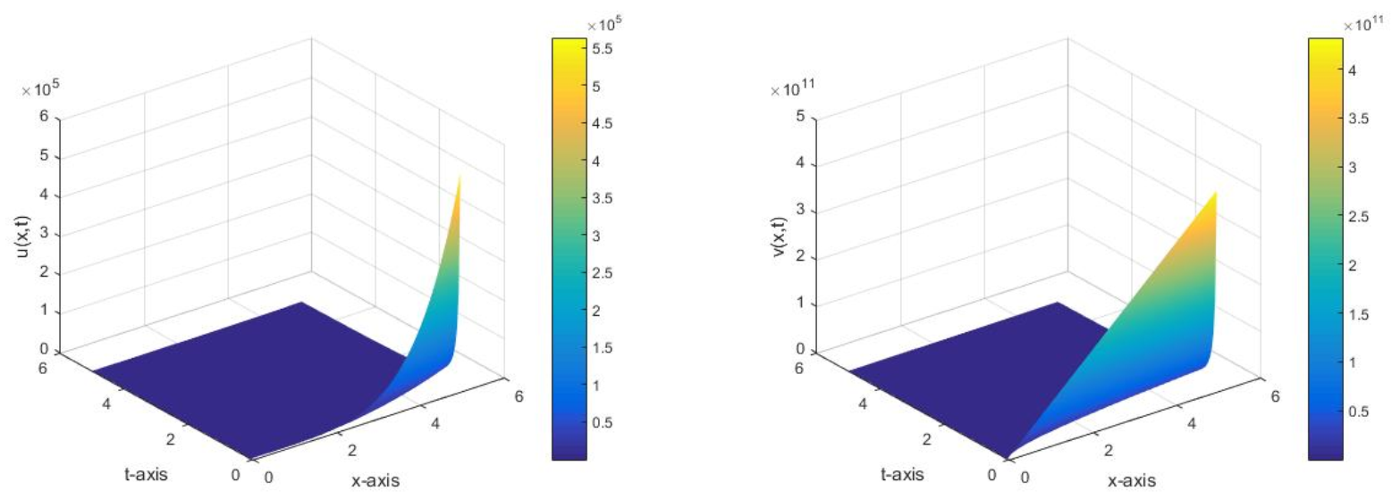
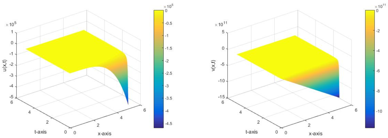
5. Series Solutions of Equations (29) and (30)

In this section, we examine the power series solution of the system. This method is more accurate and efficient for obtaining an exact analytical solution. The procedures of the method are given in [42]. We can construct

$$f\left(\xi \right)=\sum _{n=0}^{\infty }{r}_n{\xi }^n,g\left(\xi \right)=\sum _{n=0}^{\infty }{s}_n{\xi }^n,$$

(44)

$$f_{\xi }=\sum _{n=1}^{\infty }n{r}_n{\xi }^{n-1},f_{\xi \xi \xi }=\sum _{n=3}^{\infty }n(n-1)(n-2)r_n{\xi }^{n-3},$$

(45)

and

$$g_{\xi }=\sum _{n=1}^{\infty }n{s}_n{\xi }^{n-1},g_{\xi \xi \xi }=\sum _{n=3}^{\infty }n(n-1)(n-2)s_n{\xi }^{n-3}.$$

(46)

Substituting Equations (44)–(46) into Equations (29) and (30), we have

$$\begin{array}{cc}\hfill & \sum _{n=0}^{\infty }\frac{\Gamma (2-\frac{2\alpha }{3}+\frac{n\alpha }{3})}{\Gamma (2-\frac{5\alpha }{3}+\frac{n\alpha }{3})}{r}_n{\xi }^n+a_1\sum _{n=0}^{\infty }{r}_n{\xi }^n\sum _{n=0}^{\infty }(n+1)r_{n+1}{\xi }^n\hfill \\ \hfill & + b_1\sum _{n=0}^{\infty }(n+3)(n+2)(n+1)r_{n+3}{\xi }^n+cq{\left(\sum _{n=0}^{\infty }{s}_n{\xi }^n\right)}^{q-1}\sum _{n=0}^{\infty }(n+1)s_{n+1}{\xi }^n=0,\hfill \end{array}$$

(47)

and

$$\begin{array}{cc}\hfill & \sum _{n=0}^{\infty }\frac{\Gamma (2-\frac{4\alpha }{3q}+\frac{n\alpha }{3})}{\Gamma (2-\alpha -\frac{4\alpha }{3q}+\frac{n\alpha }{3})}{s}_n{\xi }^n+a_2\sum _{n=0}^{\infty }{r}_n{\xi }^n\sum _{n=0}^{\infty }(n+1)s_{n+1}{\xi }^n\hfill \\ \hfill & + b_2\sum _{n=0}^{\infty }(n+3)(n+2)(n+1)s_{n+3}{\xi }^n=0.\hfill \end{array}$$

(48)

When n = 0 in Equations (47) and (48), we obtain the following coefficients:

$$r_3=\frac{1}{6b_1}\left(\frac{\Gamma (2-\frac{2\alpha }{3})}{\Gamma (2-\frac{5\alpha }{3})}{r}_0+a_1{r}_0{r}_1+cq{s}_1^{q-1}{s}_0\right),$$

(49)

and

$$s_3=\frac{1}{6b_2}\left(\frac{\Gamma (2-\frac{4\alpha }{3q})}{\Gamma (2-\alpha -\frac{4\alpha }{3q})}{s}_0+a_2{r}_0{s}_1\right).$$

(50)

When $n⩾1$, we have the following coefficients

$$\begin{array}{cc}\hfill & r_{n+3}=\frac{1}{b_1(n+3)(n+2)(n+1)}(\frac{\Gamma (2-\frac{2\alpha }{3}+\frac{n\alpha }{3})}{\Gamma (2-\frac{5\alpha }{3}+\frac{n\alpha }{3})}{r}_n+a_1\sum _{k=0}^n(n-k+1)r_{n-k+1}{r}_k\hfill \\ \hfill & + cq\sum _{k_1=0}^n\sum _{k_2=0}^{k_1}\dots \sum _{k_{q-1}=0}^{k_{q-2}}(n-k+1)s_{n-k+1}{s}_{k_1-k_2}\dots s_{k_{q-2}-k_{q-1}{s}_{k_{q-1}}}),\hfill \end{array}$$

(51)

and

$$s_{n+3}=\frac{1}{b_2(n+3)(n+2)(n+1)}\left(\frac{\Gamma (2-\frac{4\alpha }{3q}+\frac{n\alpha }{3})}{\Gamma (2-\alpha -\frac{4\alpha }{3q}+\frac{n\alpha }{3})}{s}_n+a_2\sum _{k=0}^n(n-k+1)s_{n-k+1}{r}_k\right).$$

(52)

Thus, the coefficients $r_n$ ($n⩾1$) and $s_n$ ($n⩾1$) can be calculated for Equation (44) as arbitrary constants. This shows that there are power series solutions to the Equations (29) and (30). We then acquire the explicit power series solutions of Equation (1) (Figure 1 and Figure 2) as

$$\begin{array}{cc}\hfill & u(x,t)=r_0{t}^{\frac{-2\alpha }{3}}+r_{1}x{t}^{-\alpha }+r_2{x}^2{t}^{\frac{-4\alpha }{3}}+\frac{1}{6b_1}\left(\frac{\Gamma (2-\frac{2\alpha }{3})}{\Gamma (2-\frac{5\alpha }{3})}{r}_0+a_1{r}_0{r}_1+cq{s}_0^{q-1}{s}_1\right)x^3{t}^{\frac{-5\alpha }{3}}\hfill \\ \hfill & +\sum _{n=1}^{\infty }\frac{1}{b_1(n+3)(n+2)(n+1)}(\frac{\Gamma (2-\frac{2\alpha }{3}+\frac{n\alpha }{3})}{\Gamma (2-\frac{5\alpha }{3}+\frac{n\alpha }{3})}{r}_n+a_1\sum _{k=0}^n(n-k+1)r_{n-k+1}{r}_k\hfill \\ \hfill & + cq\sum _{k_1=0}^n\sum _{k_2=0}^{k_1}\dots \sum _{k_{q-1}=0}^{k_{q-2}}(n-k+1)s_{n-k+1}{s}_{k_1-k_2}\dots s_{k_{q-2}-k_{q-1}{s}_{k_{q-1}}})x^{n+3}{t}^{\frac{-\alpha (n+5)}{3}},\hfill \end{array}$$

(53)

$$\begin{array}{cc}\hfill & v(x,t)=s_0{t}^{\frac{-4\alpha }{3q}}+s_{1}x{t}^{\frac{-\alpha (q+4)}{3q}}+s_2{x}^2{t}^{\frac{-\alpha (2q+4)}{3q}}+\frac{1}{6b_2}\left(\frac{\Gamma (2-\frac{4\alpha }{3q})}{\Gamma (2-\alpha -\frac{4\alpha }{3q})}{s}_0+a_2{r}_0{s}_1\right)x^3{t}^{\frac{-\alpha (3q+4)}{3q}}\hfill \\ \hfill & +\sum _{n=1}^{\infty }\frac{1}{b_2(n+3)(n+2)(n+1)}\left(\frac{\Gamma (2-\frac{4\alpha }{3q}+\frac{n\alpha }{3})}{\Gamma (2-\alpha -\frac{4\alpha }{3q}+\frac{n\alpha }{3})}{s}_n+a_2\sum _{k=0}^n(n-k+1)s_{n-k+1}{r}_k\right)\hfill \\ \hfill & \times x^{n+3}{t}^{\frac{-\alpha (nq+3q+4)}{3q}}.\hfill \end{array}$$

(54)

6. Convergence Analysis of the Power Series Solution

In this part of the work, we will prove that the power series solutions (53) and (54) are convergent. Considering Equations (51) and (52), we can write

$$\begin{array}{cc}\hfill & \mid r_{n+3}\mid \le (\frac{\mid \Gamma (2-\frac{2\alpha }{3}+\frac{n\alpha }{3})\mid }{\mid \Gamma (2-\frac{5\alpha }{3}+\frac{n\alpha }{3})\mid }\mid r_n\mid +\sum _{k=0}^n\mid r_{n-k+1}\mid \mid r_k\mid \hfill \\ \hfill & +\sum _{k_1=0}^n\sum _{k_2=0}^{k_1}\dots \sum _{k_{q-1}=0}^{k_{q-2}}\mid s_{n-k+1}\mid \mid s_{k_1-k_2}\mid \dots \mid s_{k_{q-2}-k_{q-1}\mid \mid s_{k_{q-1}}\mid }),\hfill \end{array}$$

(55)

and

$$\begin{array}{c}\hfill \mid s_{n+3}\mid \le \left(\frac{\mid \Gamma (2-\frac{4\alpha }{3q}+\frac{n\alpha }{3})\mid }{\mid \Gamma (2-\alpha -\frac{4\alpha }{3q}+\frac{n\alpha }{3})\mid }\mid s_n\mid +\sum _{k=0}^n\mid s_{n-k+1}\mid \mid r_k\mid \right).\end{array}$$

(56)

Using the properties of $\Gamma$, we can easily show that $\frac{\mid \Gamma (2-\frac{2\alpha }{3}+\frac{n\alpha }{3})\mid }{\mid \Gamma (2-\frac{5\alpha }{3}+\frac{n\alpha }{3})\mid }\le 1$ and $\frac{\mid \Gamma (2-\frac{4\alpha }{3q}+\frac{n\alpha }{3})\mid }{\mid \Gamma (2-\alpha -\frac{4\alpha }{3q}+\frac{n\alpha }{3})\mid }$$\le 1$.

Therefore, we can write

$$\begin{array}{cc}\hfill & \mid r_{n+3}\mid \le M(\mid r_n\mid +\sum _{k=0}^n\mid r_{n-k+1}\mid \mid r_k\mid \hfill \\ \hfill & +\sum _{k_1=0}^n\sum _{k_2=0}^{k_1}\dots \sum _{k_{q-1}=0}^{k_{q-2}}\mid s_{n-k+1}\mid \mid s_{k_1-k_2}\mid \dots \mid s_{k_{q-2}-k_{q-1}\mid \mid s_{k_{q-1}}\mid }),\hfill \end{array}$$

(57)

and

$$\begin{array}{c}\hfill \mid s_{n+3}\mid \le N\left(\mid s_n\mid +\sum _{k=0}^n\mid s_{n-k+1}\mid \mid r_k\mid \right),\end{array}$$

(58)

where $M=max\left(\mid \frac{1}{b_1}\mid ,\mid \frac{a_1}{b_1}\mid ,\mid \frac{cq}{b_1}\mid \right)$ and $N=max\left(\mid \frac{1}{b_2}\mid ,\mid \frac{a_2}{b_2}\mid \right)$ for an arbitrary n.

We can now define another power series form as

$$K\left(\xi \right)=\sum _{n=0}^{\infty }{y}_n{\xi }^{n}andL\left(\xi \right)=\sum _{n=0}^{\infty }{z}_n{\xi }^n,$$

(59)

and let $y_i=\mid r_i\mid$ and $z_i=\mid s_i\mid$, i = 0, 1, ... . We can then easily obtain

$$\begin{array}{cc}\hfill & y_{n+3}\le M(y_n+\sum _{k=0}^n{y}_{n-k+1}{y}_k\hfill \\ \hfill & +\sum _{k_1=0}^n\sum _{k_2=0}^{k_1}\dots \sum _{k_{q-1}=0}^{k_{q-2}}{z}_{n-k+1}{z}_{k_1-k_2}\dots z_{k_{q-2}-k_{q-1}{z}_{k_{q-1}}}),\hfill \end{array}$$

(60)

and

$$\begin{array}{c}\hfill z_{n+3}\le N\left(z_n+\sum _{k=0}^n{z}_{n-k+1}{y}_k\right),\end{array}$$

(61)

Thus, it is obvious that $\mid y_n\mid \le r_n$ and $\mid z_n\mid \le s_n$ for n = 0, 1, 2, .... This also confirms that the series Equation (59) are the majorant series of Equation (44). We now have to prove that the series $K(\xi$) and $L\left(\xi \right)$ have positive radius of convergence. By elementary calculations, we have the following:

$$\begin{array}{cc}\hfill & K\left(\xi \right)=y_0+y_1\xi +y_2{\xi }^2+y_3{\xi }^3+M(\sum _{n=0}^{\infty }{y}_n+\sum _{n=0}^{\infty }\sum _{k=0}^n{y}_{n-k+1}{y}_k\hfill \\ \hfill & +\sum _{n=0}^{\infty }\sum _{k_1=0}^n\sum _{k_2=0}^{k_1}\dots \sum _{k_{q-1}=0}^{k_{q-2}}{z}_{n-k+1}{z}_{k_1-k_2}\dots z_{k_{q-2}-k_{q-1}{z}_{k_{q-1}}}){\xi }^{n+3},\hfill \end{array}$$

(62)

and

$$\begin{array}{c}\hfill L\left(\xi \right)=z_0+z_1\xi +z_2{\xi }^2+z_3{\xi }^3+N\left(\sum _{n=0}^{\infty }{z}_n+\sum _{n=0}^{\infty }\sum _{k=0}^n{z}_{n-k+1}{y}_k\right){\xi }^{n+3}.\end{array}$$

(63)

We can take into account an implicit functional system with respect to the independent variable $\xi$ as follows:

$$\mathcal{K}(\xi ,K)=K-y_0-y_1\xi -y_2{\xi }^2-y_3{\xi }^3-M\left({\xi }^2(K-y_0)+{\xi }^{2}K(K-y_0)+{\xi }^{2}L{(L-z_0)}^{q-2}\right),$$

(64)

and

$$\mathcal{L}(\xi ,L)=L-z_0-z_1\xi -z_2{\xi }^2-z_3{\xi }^3-N\left({\xi }^2(L-z_0)+{\xi }^{2}L(K-y_0)\right).$$

(65)

It is clear that $\mathcal{K}$ and $\mathcal{L}$ are analytical in the neighborhood of $(0,y_0)$ and $(0,z_0)$. Therefore, $\mathcal{K}(0,y_0)=0$, $\mathcal{L}(0,z_0)=0$, and $\frac{\partial }{\partial K}\mathcal{K}(0,y_0)\ne 0$, $\frac{\partial }{\partial L}\mathcal{L}(0,z_0)\ne 0$ According to the implicit function theorem [43], the convergence is proved.

7. Conclusions

In this paper, we used a Lie point symmetry method in order to reduce a time fractional generalized coupled Drinfeld-Sokolov system to a time fractional coupled ODE system with the aid of the Riemann Liouville derivative and the fractional EK differential operator. By using the İbragimov conservation theorem, we obtained conservation vectors of the system. We then acquired explicit exact solutions of the reduced time fractional coupled ODE system by using a power series expansion method and proved that the series solutions are convergent.

References

1. Diethelm, K. The Analysis of Fractional Differential Equations; Springer: Berlin, Germany, 2010. [Google Scholar]
2. Miller, K.S.; Ross, B. An Introduction To the Fractional Calculus and Fractional Differential Equations; Wiley: New York, NY, USA, 1993. [Google Scholar]
3. Podlubny, I. Fractional Differential Equations; Academic Press: San Diego, CA, USA, 1999. [Google Scholar]
4. Oldham, K.B.; Spanier, J. The Fractional Calculus; Academic Press: San Diego, CA, USA, 1974. [Google Scholar]
5. Guy, J. Lagrange characteristic method for solving a class of nonlinear partial differential equations of fractional order. Appl. Math. Lett. 2006, 19, 873–880. [Google Scholar] [CrossRef] [Green Version]
6. El-Sayed, A.; Gaber, M. The Adomian decomposition method for solving partial differential equations of fractal order in finite domains. Phys. Lett. A 2006, 359, 175–182. [Google Scholar] [CrossRef]
7. Baleanu, D.; Inc, M.; Yusuf, A.; Aliyu, A.I. Institute of Space Sciences Lie symmetry analysis, exact solutions and conservation laws for the time fractional modified Zakharov–Kuznetsov equation. Nonlinear Anal. Model. Control. 2017, 22, 861–876. [Google Scholar] [CrossRef]
8. Jumarie, G. Cauchy’s integral formula via the modified Riemann–Liouville derivative for analytic functions of fractional order. Appl. Math. Lett. 2010, 23, 1444–1450. [Google Scholar] [CrossRef] [Green Version]
9. Sardar, A.; Husnine, S.M.; Rizvi, S.T.R.; Younis, M.; Ali, K. Multiple travelling wave solutions for electrical transmission line model. Nonlinear Dyn. 2015, 82, 1317–1324. [Google Scholar] [CrossRef]
10. Ali, S.; Rizvi, S.T.R.; Younis, M. Traveling wave solutions for nonlinear dispersive water-wave systems with time-dependent coefficients. Nonlinear Dyn. 2015, 82, 1755–1762. [Google Scholar] [CrossRef]
11. Cheemaa, N.; Younis, M. New and more exact traveling wave solutions to integrable (2 + 1)-dimensional Maccari system. Nonlinear Dyn. 2016, 83, 1395–1401. [Google Scholar] [CrossRef]
12. Cheemaa, N.; Younis, M. New and more general traveling wave solutions for nonlinear Schrodinger equation. Waves Random Complex Media 2016, 26, 84–91. [Google Scholar] [CrossRef]
13. Deng, W. Finite Element Method for the Space and Time Fractional Fokker–Planck Equation. SIAM J. Numer. Anal. 2009, 47, 204–226. [Google Scholar] [CrossRef]
14. Zhang, S. Application of Exp-function method to a KdV equation with variable coefficients. Phys. Lett. A 2007, 365, 448–453. [Google Scholar] [CrossRef]
15. Zhang, X.; Zhao, J.; Liu, J.; Tang, B. Homotopy perturbation method for two dimensional time-fractional wave equation. Appl. Math. Model. 2014, 38, 5545–5552. [Google Scholar] [CrossRef]
16. Fadravi, H.H.; Nik, H.S.; Buzhabadi, R. Homotopy Analysis Method for Solving Foam Drainage Equation with Space- and Time-Fractional Derivatives. Int. J. Differ. Equ. 2011, 2011, 1–12. [Google Scholar] [CrossRef] [Green Version]
17. Gurefe, Y.; Sonmezoglu, A.; Misirli, E. Application of the trial equation method for solving some nonlinear evolution equations arising in mathematical physics. Pramana 2011, 77, 1023–1029. [Google Scholar] [CrossRef]
18. Zheng, B.; Wen, C. Exact solutions for fractional partial differential equations by a new fractional sub-equation method. Adv. Differ. Equ. 2013, 2013, 199. [Google Scholar] [CrossRef] [Green Version]
19. Kumar, S.; Kour, B.; Yao, S.-W.; Inc, M.; Osman, M. Invariance Analysis, Exact Solution and Conservation Laws of (2 + 1) Dim Fractional Kadomtsev-Petviashvili (KP) System. Symmetry 2021, 13, 477. [Google Scholar] [CrossRef]
20. Kour, B.; Kumar, S. Space time fractional Drinfel’d-Sokolov-Wilson system with time-dependent variable coefficients: Symmetry analysis, power series solutions and conservation laws. Eur. Phys. J. Plus 2019, 134, 1–15. [Google Scholar] [CrossRef]
21. Lukashchuk, S.Y. Symmetry reduction and invariant solutions for nonlinear fractional diffusion equation with a source term. Ufim. Mat. Zhurnal 2016, 8, 111–122. [Google Scholar] [CrossRef]
22. Lie, S. Theorie der Transformationsgruppen II; Written with the help of Friedrich Engel; BG Teubner: Leipzig, Germany, 1890. [Google Scholar]
23. Bluman, G.W.; Kumei, S. Symmetries and Differential Equations; Springer Science and Business Media: Berlin, Germany, 2013; Volume 81. [Google Scholar]
24. Ibragimov, N.K. Elementary Lie Group Analysis and Ordinary Differential Equations; Wiley: New York, NY, USA, 1999; Volume 197. [Google Scholar]
25. Clarkson, P.A.; Kruskal, M.D. New similarity reductions of the Boussinesq equation. J. Math. Phys. 1989, 30, 2201–2213. [Google Scholar] [CrossRef]
26. Clarkson, P.A. New similarity solutions for the modified Boussinesq equation. J. Phys. A Math. Gen. 1989, 22, 2355–2367. [Google Scholar] [CrossRef]
27. Noether, E. Invariant variation problems. Transp. Theory Stat. Phys. 1971, 1, 186–207. [Google Scholar] [CrossRef] [Green Version]
28. Atanacković, T.M.; Konjik, S.; Pilipović, S.; Simić, S. Variational problems with fractional derivatives: Invariance conditions and Noether’s theorem. Nonlinear Anal. Theory Methods Appl. 2009, 71, 1504–1517. [Google Scholar] [CrossRef] [Green Version]
29. Ibragimov, N.H. A new conservation theorem. J. Math. Anal. Appl. 2007, 333, 311–328. [Google Scholar] [CrossRef] [Green Version]
30. Lukashchuk, S.Y. Conservation laws for time-fractional sub diffusion and diffusion-wave equations. Nonlinear Dyn. 2015, 80, 791–802. [Google Scholar] [CrossRef] [Green Version]
31. Coclite, G.M.; Dipierro, S.; Maddalena, F.; Valdinoci, E. Singularity Formation in Fractional Burgers’ Equations. J. Nonlinear Sci. 2020, 30, 1285–1305. [Google Scholar] [CrossRef] [Green Version]
32. Kirane, M.; Malik, S.A. The profile of blowing-up solutions to a nonlinear system of fractional differential equations. Nonlinear Anal. Theory Methods Appl. 2010, 73, 3723–3736. [Google Scholar] [CrossRef] [Green Version]
33. Miškinis, P. Some properties of fractional burgers equation. Math. Model. Anal. 2002, 7, 151–158. [Google Scholar] [CrossRef] [Green Version]
34. Sahoo, S.; Ray, S.S. Invariant analysis with conservation laws for the time fractional Drinfeld–Sokolov–Satsuma–Hirota equations. Chaos Solitons Fractals 2017, 104, 725–733. [Google Scholar] [CrossRef]
35. Jumarie, G. Modified Riemann-Liouville derivative and fractional Taylor series of nondifferentiable functions further results. Comput. Math. Appl. 2006, 51, 1367–1376. [Google Scholar] [CrossRef] [Green Version]
36. Gazizov, R.K.; A Kasatkin, A.; Lukashchuk, S.Y. Symmetry properties of fractional diffusion equations. Phys. Scr. 2009, T136, 14–16. [Google Scholar] [CrossRef]
37. Kiryakova, V.S. Generalized Fractional Calculus and Applications; CRC Press: Boca Raton, FL, USA, 1993. [Google Scholar]
38. Huang, Q.; Zhdanov, R. Symmetries and exact solutions of the time fractional Harry-Dym equation with Riemann–Liouville derivative. Phys. A Stat. Mech. Its Appl. 2014, 409, 110–118. [Google Scholar] [CrossRef]
39. Wang, G.-W.; Xu, T.-Z. Invariant analysis and exact solutions of nonlinear time fractional Sharma–Tasso–Olver equation by Lie group analysis. Nonlinear Dyn. 2013, 76, 571–580. [Google Scholar] [CrossRef]
40. Gazizov, R.; Ibragimov, N.; Lukashchuk, S. Nonlinear self-adjointness, conservation laws and exact solutions of time-fractional Kompaneets equations. Commun. Nonlinear Sci. Numer. Simul. 2015, 23, 153–163. [Google Scholar] [CrossRef]
41. Hashemi, M. Group analysis and exact solutions of the time fractional Fokker–Planck equation. Phys. A Stat. Mech. Its Appl. 2015, 417, 141–149. [Google Scholar] [CrossRef]
42. Nuseir, A.S.; Al-Hasson, A. Power series solution for nonlinear system of partial differential equations. Appl. Math. Sci. 2012, 6, 5147–5159. [Google Scholar]
43. Rudin, W. Principles of Mathematical Analysis; McGraw-Hill: New York, NY, USA, 1976; Volume 3. [Google Scholar]
Figure 1. 3-D plots of Equations (53) and (54) with r 0 = 1 , r 1 = 2 , r 2 = 3 , s 0 = s 1 = s 2 = 2 , b 1 = b 2 = 1 , a 1 = a 2 = 2 , q = 2 , c = 2 and α = 0.5 .
Symmetry 13 00874 g001
Figure 2. 3-D plots of Equations (53) and (54) with r 0 = 2 , r 1 = 2 , r 2 = 2 , s 0 = s 1 = s 2 = 1 , b 1 = 1 , b 2 = 6 , a 1 = 6 , a 2 = 2 , q = 1 , c = 6 and α = 0.75 .
Symmetry 13 00874 g002
Publisher’s Note: MDPI stays neutral with regard to jurisdictional claims in published maps and institutional affiliations.