Explicit Identities for 3-Variable Degenerate Hermite Kampé de Fériet Polynomials and Differential Equation Derived from Generating Function

Abstract

We get the 3-variable degenerate Hermite Kampé de Fériet polynomials and get symmetric identities for 3-variable degenerate Hermite Kampé de Fériet polynomials. We make differential equations coming from the generating functions of degenerate Hermite Kampé de Fériet polynomials to get some identities for 3-variable degenerate Hermite Kampé de Fériet polynomials,. Finally, we study the structure and symmetry of pattern about the zeros of the 3-variable degenerate Hermite Kampé de Fériet equations.

1. Introduction

The classical Hermite numbers $H_n$ and polynomials $H_n\left(x\right)$ are usually defined by the generating functions

$$e^{-t^2}=\sum _{n=0}^{\infty }{H}_n{\displaystyle \frac{t^n}{n!}},$$

(1)

and

$$e^{2xt-t^2}=\sum _{n=0}^{\infty }{H}_n\left(x\right){\displaystyle \frac{t^n}{n!}}.$$

(2)

Clearly, $H_n=H_n\left(0\right)$.

These numbers and polynomials have been studied because of important roles in many areas of mathematics (see References [1,2]). The special polynomials of 3-variable give partial differential equations of physical phenomenon. Physical problems was expressed by the special functions of mathematical physics. We recall that the 3-variable Hermite polynomials $H_n(x,y,z)$ made by the generating function (see Reference [3])

$$\sum _{n=0}^{\infty }{H}_n(x,y,z){\displaystyle \frac{t^n}{n!}}=e^{xt+y{t}^2+z{t}^3}$$

(3)

are solutions in the system of equations

$$\begin{gathered} {\displaystyle \frac{\partial }{\partial y}}{H}_n(x,y,z)={\displaystyle \frac{{\partial }^2}{\partial x^2}}{H}_n(x,y,z), \\ {\displaystyle \frac{\partial }{\partial z}}{H}_n(x,y,z)={\displaystyle \frac{{\partial }^3}{\partial x^3}}{H}_n(x,y,z), \\ {H}_n(x,0,0)=x^n. \end{gathered}$$

In particular, one has

$$H_n(2x,-1,0)=H_n\left(x\right).$$

Many researchers studied special numbers and polynomials because of importance (see References [1,2,3,4,5,6,7]). The degenerate Bernoulli, Euler, Genocchi and tangent polynomials were studied in several papers (see References [8,9,10,11,12]). Recently, researchers have studied the differential equations which are related to generating functions of special polynomials (see References [13,14,15,16,17,18]).

We construct the 3-variable degenerate Hermite Kampé de Fériet polynomials and get symmetric identities for 3-variable degenerate Hermite Kampé de Fériet polynomials. Finally, we study the distribution and symmetry of pattern of the roots of the 3-variable degenerate Hermite Kampé de Fériet polynomials Hermite equations.

We define the 3-variable degenerate Hermite Kampé de Fériet polynomials ${\mathbf{H}}_n(x,y,z|\mu )$ made by the generating function

$$\mathfrak{F}(t,x,y,z|\mu )=\sum _{n=0}^{\infty }{\mathbf{H}}_n(x,y,z|\mu ){\displaystyle \frac{t^n}{n!}}={(1+\mu )}^{{\displaystyle \frac{xt}{\mu }}}{(1+\mu )}^{{\displaystyle \frac{y{t}^2}{\mu }}}{(1+\mu )}^{{\displaystyle \frac{z{t}^3}{\mu }}}.$$

(4)

Since ${(1+\mu )}^{\frac{t}{\mu }}\to e^t$ as $\mu \to 0$, it is clear that (4) reduces to (3). If $\mu \to 0$ and $z=0$, Equation (4) is the generating function of the 2-variable Hermite polynomials $H_n(x,y,0)$. Observe that Hermite polynomials $H_n(x,y,0)$ with the 2-variable are the solution of the heat equation (see Reference [17])

$${\displaystyle \frac{\partial }{\partial y}}{H}_n(x,y,0)={\displaystyle \frac{{\partial }^2}{\partial x^2}}{H}_n(x,y,0),H_n(x,0,0)=x^n.$$

Theorem 1.

For $n=0,1,...$, the 3-variable degenerate Hermite Kampé de Fériet polynomials ${\mathbf{H}}_n(x,y,z|\mu )$ with the generating function (4) are the solution of the differential equation

$$\begin{array}{cc}& \left(3z{\displaystyle \frac{{\partial }^2}{\partial x\partial y}}+2y{\displaystyle \frac{{\partial }^2}{\partial x^2}}+x{\displaystyle \frac{log(1+\mu )}{\mu }}{\displaystyle \frac{\partial }{\partial x}}-n{\displaystyle \frac{log(1+\mu )}{\mu }}\right){\mathbf{H}}_n(x,y,z|\mu )=0,\hfill \\ & {\mathbf{H}}_n(x,0,0|\mu )={\left({\displaystyle \frac{log(1+\mu )}{\mu }}\right)}^n{x}^n.\hfill \\ & {\mathbf{H}}_n(0,y,0|\mu )=\left\{\begin{array}{cc}{\left({\displaystyle \frac{log(1+\mu )}{\mu }}\right)}^k{y}^k{\displaystyle \frac{\left(2k\right)!}{k!}},\hfill & \mathrm{if}n=2k\hfill \\ 0,\hfill & \mathrm{otherwise}\hfill \end{array}\right.\hfill \\ & {\mathbf{H}}_n(0,0,z|\mu )=\left\{\begin{array}{cc}{\left({\displaystyle \frac{log(1+\mu )}{\mu }}\right)}^k{z}^k{\displaystyle \frac{\left(3k\right)!}{k!}},\hfill & \mathrm{if}n=3k\hfill \\ 0,\hfill & \mathrm{otherwise}\hfill \end{array}\right.\hfill \end{array}$$

Proof. 

We see that

$$\mathfrak{F}(t,x,y,z|\mu )={(1+\mu )}^{{\displaystyle \frac{xt}{\mu }}}{(1+\mu )}^{{\displaystyle \frac{y{t}^2}{\mu }}}{(1+\mu )}^{{\displaystyle \frac{z{t}^3}{\mu }}}$$

satisfies

$${\displaystyle \frac{\partial \mathfrak{F}(t,x,y,z|\mu )}{\partial t}}-{\displaystyle \frac{log(1+\mu )}{\mu }}\left(x+2yt+3z{t}^2\right)\mathfrak{F}(t,x,y,z|\mu )=0.$$

By substituting the series (4) for $\mathfrak{F}(t,x,y,z|\mu )$, one obtains

$$\begin{array}{cc}& {\mathbf{H}}_{n+1}(x,y,z|\mu )-x{\displaystyle \frac{log(1+\mu )}{\mu }}{\mathbf{H}}_n(x,y,z|\mu )-2y{\displaystyle \frac{log(1+\mu )}{\mu }}{\mathbf{H}}_{n-1}(x,y,z|\mu )\hfill \\ & -n(n-1)3z{\displaystyle \frac{log(1+\mu )}{\mu }}{\mathbf{H}}_{n-2}(x,y,z|\mu )=0,n=2,3,\dots \hfill \end{array}$$

(5)

We get a recurrence relation for 3-variable degenerate Hermite Kampé de Fériet polynomials and another recurrence relation which comes from

$${\displaystyle \frac{\partial \mathfrak{F}(t,x,y,z|\mu )}{\partial x}}-{\displaystyle \frac{log(1+\mu )}{\mu }}t\mathfrak{F}(t,x,y,z|\mu )=0.$$

This implies

$${\displaystyle \frac{\partial {\mathbf{H}}_n(x,y,z|\mu )}{\partial x}}-n{\displaystyle \frac{log(1+\mu )}{\mu }}{\mathbf{H}}_{n-1}(x,y,z|\mu )=0,n=1,2,\dots$$

(6)

On the other hand, since

$${\displaystyle \frac{\partial \mathfrak{F}(t,x,y,z|\mu )}{\partial y}}-{\displaystyle \frac{log(1+\mu )}{\mu }}{t}^2\mathfrak{F}(t,x,y,z|\mu )=0,$$

we get

$${\displaystyle \frac{\partial {\mathbf{H}}_n(x,y,z|\mu )}{\partial y}}-n(n-1){\displaystyle \frac{log(1+\mu )}{\mu }}{\mathbf{H}}_{n-2}(x,y,z|\mu )=0,n=2,3,\dots$$

(7)

Eliminate ${\mathbf{H}}_{n-1}(x,y,z|\mu )$ and ${\mathbf{H}}_{n-2}(x,y,z|\mu )$ from (5)–(7) to obtain

$${\mathbf{H}}_{n+1}(x,y,z|\mu )-x{\displaystyle \frac{log(1+\mu )}{\mu }}{\mathbf{H}}_n(x,y,z|\mu )-2y{\displaystyle \frac{\partial {\mathbf{H}}_n(x,y,z|\mu )}{\partial x}}-3z{\displaystyle \frac{\partial {\mathbf{H}}_n(x,y,z|\mu )}{\partial y}}=0.$$

Differentiate this equation and use (6) again to get

$$\begin{array}{cc}& 3z{\displaystyle \frac{{\partial }^2{\mathbf{H}}_n(x,y,z|\mu )}{\partial x\partial y}}+2y{\displaystyle \frac{\partial {\mathbf{H}}_n(x,y,z|\mu )}{\partial x}}+x{\displaystyle \frac{log(1+\mu )}{\mu }}{\mathbf{H}}_n(x,y,z|\mu )\hfill \\ & -n{\displaystyle \frac{log(1+\mu )}{\mu }}{\mathbf{H}}_n(x,y,z|\mu )=0,(n=0,1,\dots ),\hfill \end{array}$$

(8)

thus we have shown the theorem. □

Theorem 2.

The 3-variable degenerate Hermite Kampé de Fériet polynomials ${\mathbf{H}}_n(x,y,z|\mu )$ with the generating function (4) are the solution of the differential equation

$$\begin{array}{cc}& \left(3z{\displaystyle \frac{\mu }{log(1+\mu )}}{\displaystyle \frac{{\partial }^3}{\partial x^3}}+2y{\displaystyle \frac{{\partial }^2}{\partial x^2}}+x{\displaystyle \frac{log(1+\mu )}{\mu }}{\displaystyle \frac{\partial }{\partial x}}-n{\displaystyle \frac{log(1+\mu )}{\mu }}\right){\mathbf{H}}_n(x,y,z|\mu )=0,\hfill \\ & {\mathbf{H}}_n(x,0,0|\mu )={\left({\displaystyle \frac{log(1+\mu )}{\mu }}\right)}^n{x}^n,n=0,1,2,\dots .\hfill \\ & {\mathbf{H}}_n(0,y,0|\mu )=\left\{\begin{array}{cc}{\left({\displaystyle \frac{log(1+\mu )}{\mu }}\right)}^k{y}^k{\displaystyle \frac{\left(2k\right)!}{k!}},\hfill & \mathrm{if}n=2k\hfill \\ 0,\hfill & \mathrm{otherwise}\hfill \end{array}\right.\hfill \\ & {\mathbf{H}}_n(0,0,z|\mu )=\left\{\begin{array}{cc}{\left({\displaystyle \frac{log(1+\mu )}{\mu }}\right)}^k{z}^k{\displaystyle \frac{\left(3k\right)!}{k!}},\hfill & \mathrm{if}n=3k\hfill \\ 0,\hfill & \mathrm{otherwise}.\hfill \end{array}\right.\hfill \end{array}$$

Proof. 

We get another recurrence relation which comes from

$${\displaystyle \frac{{\partial }^2\mathfrak{F}(t,x,y,z|\mu )}{\partial x\partial y}}-{\left({\displaystyle \frac{log(1+\mu )}{\mu }}\right)}^2{t}^2\mathfrak{F}(t,x,y,z|\mu )=0.$$

This implies

$${\displaystyle \frac{{\partial }^2{\mathbf{H}}_n(x,y,z|\mu )}{\partial x\partial y}}=n(n-1)(n-2){\left({\displaystyle \frac{log(1+\mu )}{\mu }}\right)}^2{\mathbf{H}}_{n-3}(x,y,z|\mu )=0,n=3,4,\dots$$

(9)

Again, we also have

$${\displaystyle \frac{{\partial }^3\mathfrak{F}(t,x,y,z|\mu )}{\partial x^3}}-{\left({\displaystyle \frac{log(1+\mu )}{\mu }}\right)}^3{t}^3\mathfrak{F}(t,x,y,z|\mu )=0.$$

This implies

$${\displaystyle \frac{{\partial }^3{\mathbf{H}}_n(x,y,z|\mu )}{\partial x^3}}=n(n-1)(n-2){\left({\displaystyle \frac{log(1+\mu )}{\mu }}\right)}^3{\mathbf{H}}_{n-3}(x,y,z|\mu )=0,n=3,4,\dots$$

(10)

Thus, from (8)–(10), the degenerate Hermite Kampé de Fériet polynomials ${\mathbf{H}}_n(x,y,z|\mu )$ of 3-variable with the generating function (4) are the solution of the differential equation

$$\begin{array}{cc}& {\displaystyle \frac{3z\mu }{log(1+\mu )}}{\displaystyle \frac{{\partial }^3{\mathbf{H}}_n(x,y,z|\mu )}{\partial x^3}}+2y{\displaystyle \frac{{\partial }^2{\mathbf{H}}_n(x,y,z|\mu )}{\partial x^2}}\hfill \\ & +x{\displaystyle \frac{log(1+\mu )}{\mu }}{\displaystyle \frac{\partial {\mathbf{H}}_n(x,y,z|\mu )}{\partial x}}-n{\displaystyle \frac{log(1+\mu )}{\mu }}{\mathbf{H}}_n(x,y,z|\mu )=0.\hfill \end{array}$$

Therefore, we are done. □

We see another application of the differential equation for ${\mathbf{H}}_n(x,y,z|\mu )$. The polynomials ${\mathbf{H}}_n(x,y,z|\mu )$ have this relations

$$\begin{array}{cc}& {\displaystyle \frac{\partial {\mathbf{H}}_n(x,y,z|\mu )}{\partial y}}-{\displaystyle \frac{\mu }{log(1+\mu )}}{\displaystyle \frac{{\partial }^2{\mathbf{H}}_n(x,y,z|\mu )}{\partial x^2}}=0,\hfill \\ & {\displaystyle \frac{\partial {\mathbf{H}}_n(x,y,z|\mu )}{\partial z}}-{\left({\displaystyle \frac{\mu }{log(1+\mu )}}\right)}^2{\displaystyle \frac{{\partial }^2{\mathbf{H}}_n(x,y,z|\mu )}{\partial x^2}}=0,\hfill \end{array}$$

which in view of the initial condition are solved by

$$\begin{array}{c}{\mathbf{H}}_n(x,0,0|\mu )={\left({\displaystyle \frac{log(1+\mu )}{\mu }}\right)}^n{x}^n,n=0,1,2,\dots .\hfill \\ {\mathbf{H}}_n(0,y,0|\mu )=\left\{\begin{array}{cc}{\left({\displaystyle \frac{log(1+\mu )}{\mu }}\right)}^k{y}^k{\displaystyle \frac{\left(2k\right)!}{k!}},\hfill & \mathrm{if}n=2k\hfill \\ 0,\hfill & \mathrm{otherwise}\hfill \end{array}\right.\hfill \\ {\mathbf{H}}_n(0,0,z|\mu )=\left\{\begin{array}{cc}{\left({\displaystyle \frac{log(1+\mu )}{\mu }}\right)}^k{z}^k{\displaystyle \frac{\left(3k\right)!}{k!}},\hfill & \mathrm{if}n=3k\hfill \\ 0,\hfill & \mathrm{otherwise}\hfill \end{array}\right.\hfill \end{array}$$

The Stirling numbers of the first kind, $S_1(n,k)$, were defined by (see References [8,9,10])

$${\left(x\right)}_n=\sum _{k=0}^n{S}_1(n,k)x^k.$$

$S_1(n,k)$ is

$$\sum _{n=m}^{\infty }{S}_1(n,m){\displaystyle \frac{t^n}{n!}}={\displaystyle \frac{1}{m!}}{(log(1+t))}^m,$$

where ${\left(x\right)}_n=x(x-1)\cdots (x-n+1)$. We see the binomial theorem: for a variable x,

$$\begin{array}{cc}\hfill {(1+\mu )}^{{\displaystyle \frac{xt}{\mu }}}& =\sum _{m=0}^{\infty }{\left({\displaystyle \frac{tx}{\mu }}\right)}_m{\displaystyle \frac{{\mu }^m}{m!}}\hfill \\ & =\sum _{m=0}^{\infty }\left(\sum _{l=0}^m{S}_1(m,l){\left({\displaystyle \frac{tx}{\mu }}\right)}^l{\displaystyle \frac{{\mu }^m}{m!}}\right)\hfill \\ & =\sum _{l=0}^{\infty }\left(\sum _{m=l}^{\infty }{S}_1(m,l)x^l{\mu }^{m-l}{\displaystyle \frac{l!}{m!}}\right){\displaystyle \frac{t^l}{l!}}.\hfill \end{array}$$

(11)

By (4), we have

$$\begin{array}{cc}& \sum _{n=0}^{\infty }{\mathbf{H}}_n(x,y,z|\mu ){\displaystyle \frac{t^n}{n!}}={(1+\mu )}^{{\displaystyle \frac{xt}{\mu }}}{(1+\mu )}^{{\displaystyle \frac{y{t}^2}{\mu }}}{(1+\mu )}^{{\displaystyle \frac{z{t}^2}{\mu }}}\hfill \\ & =\sum _{k=0}^{\infty }{\left({\displaystyle \frac{ylog(1+\mu )}{\mu }}\right)}^k{\displaystyle \frac{t^{2k}}{k!}}\sum _{l=0}^{\infty }{\left({\displaystyle \frac{xlog(1+\mu )}{\mu }}\right)}^l{\displaystyle \frac{t^l}{l!}}\sum _{j=0}^{\infty }{\left({\displaystyle \frac{xlog(1+\mu )}{\mu }}\right)}^j{\displaystyle \frac{t^{3j}}{j!}}\hfill \\ & =\sum _{n=0}^{\infty }\left(\sum _{k=0}^{\left[\frac{n}{2}\right]}{\left({\displaystyle \frac{log(1+\mu )}{\mu }}\right)}^{n-k}{y}^k{x}^{n-2k}{\displaystyle \frac{n!}{k!(n-2k)!}}\right){\displaystyle \frac{t^n}{n!}}\sum _{j=0}^{\infty }{\left({\displaystyle \frac{xlog(1+\mu )}{\mu }}\right)}^j{\displaystyle \frac{t^{3j}}{j!}}\hfill \\ & \sum _{n=0}^{\infty }\left(\sum _{k=0}^{\left[\frac{n}{3}\right]}\sum _{l=0}^{\left[\frac{n-3k}{2}\right]}{\left({\displaystyle \frac{log(1+\mu )}{\mu }}\right)}^{n-2k-l}{\displaystyle \frac{z^k{y}^l{x}^{n-3k-2l}n!(n-3k)!}{k!l!(n-3k)!(n-3k-2l)!}}\right){\displaystyle \frac{t^n}{n!}}.\hfill \end{array}$$

(12)

If we compare the coefficients $\frac{t^n}{n!}$ on the both sides of (12), we have representation of ${\mathbf{H}}_n(x,y,z|\mu )$.

$${\mathbf{H}}_n(x,y,z|\mu )=\sum _{k=0}^{\left[\frac{n}{3}\right]}\sum _{l=0}^{\left[\frac{n-3k}{2}\right]}{\left({\displaystyle \frac{log(1+\mu )}{\mu }}\right)}^{n-2k-l}{\displaystyle \frac{z^k{y}^l{x}^{n-3k-2l}n!(n-3k)!}{k!l!(n-3k)!(n-3k-2l)!}},$$

and $\left[\right]$ denotes taking the integer part.

The following elementary properties of ${\mathbf{H}}_n(x,y,z|\mu )$ are deduced form (4). We delete the details.

Theorem 3.

For any positive n, we have

$$\begin{array}{c}1.{\mathbf{H}}_n(x,0,0|\mu )=\sum _{m=n}^{\infty }{S}_1(m,n)x^n{\mu }^{m-n}{\displaystyle \frac{n!}{m!}}.\hfill \\ 2.{\mathbf{H}}_n(x_1+x_2,y,z|\mu )=\sum _{l=0}^n\sum _{m=l}^{\infty }\left(\genfrac{}{}{0pt}{}{n}{l}\right){\mathbf{H}}_{n-l}(x_1,y,z|\mu )S_1(m,l)x_2^l{\mu }^{m-l}{\displaystyle \frac{l1}{m!}}.\hfill \\ 3.{\mathbf{H}}_n(x,y_1+y_2,z|\mu )=\sum _{k=0}^{\left[\frac{n}{2}\right]}{\mathbf{H}}_{n-2k}(x,y_1,z|\mu ){\left({\displaystyle \frac{log(1+\mu )}{\mu }}\right)}^k{y}_2^k{\displaystyle \frac{n!}{k!(n-2k)!}}.\hfill \\ 4.{\mathbf{H}}_n(x,y_1+y_2,z|\mu )=\sum _{k=0}^{\left[\frac{n}{2}\right]}\sum _{m=k}^{\infty }{\displaystyle \frac{S_1(m,k)y_2^k{\mu }^{m-k}n!}{m!(n-2k)!}}{\mathbf{H}}_{n-2k}(x,y_1,z|\mu ).\hfill \\ 5.{\mathbf{H}}_n(x,y,z_1+z_2|\mu )=\sum _{k=0}^{\left[\frac{n}{3}\right]}{\mathbf{H}}_{n-3k}(x,y,z_1|\mu ){\left({\displaystyle \frac{log(1+\mu )}{\mu }}\right)}^k{z}_2^k{\displaystyle \frac{n!}{k!(n-3k)!}}.\hfill \\ 6.{\mathbf{H}}_n(x,y,z_1+z_2|\mu )=\sum _{k=0}^{\left[\frac{n}{3}\right]}\sum _{m=k}^{\infty }{\displaystyle \frac{S_1(m,k)z_2^k{\mu }^{m-k}n!}{m!(n-3k)!}}{\mathbf{H}}_{n-3k}(x,y,z_1|\mu ).\hfill \\ 7.{\mathbf{H}}_n(x_1+x_2,y_1+y_2,z_1+z_2|\mu )=\sum _{l=0}^n\left(\genfrac{}{}{0pt}{}{n}{l}\right){\mathbf{H}}_l(x_1,y_1,z_1|\mu ){\mathbf{H}}_{n-l}(x_2,y_2,z_2|\mu ).\hfill \end{array}$$

The paper is written by this process: We make symmetric identities about 3-variable degenerate Hermite Kampé de Fériet polynomials in Section 2. We also get formulas of 3-variable degenerate Hermite Kampé de Fériet polynomials. We induce the differential equations getting from the generating function of 3-variable degenerate Hermite Kampé de Fériet polynomials in Section 3:

$$\begin{array}{cc}& {\left({\displaystyle \frac{\partial }{\partial t}}\right)}^N\mathfrak{F}(t,x,y,z|\mu )-a_0(N,x,y,z|\mu )\mathfrak{F}(t,x,y,z|\mu )-a_1(N,x,y,z|\mu )t\mathfrak{F}(t,x,y,z|\mu )-\cdots \hfill \\ & -a_{N-1}(N,x,y,z|\mu )t^{N-1}\mathfrak{F}(t,x,y,z|\mu )-a_N(N,x,y,z|\mu )t^N\mathfrak{F}(t,x,y,z|\mu )=0.\hfill \end{array}$$

In Section 4, we study distribution of computer graphic about the roots of the 3-variable degenerate Hermite Kampé de Fériet equation ${\mathbf{H}}_n(x,y,z|\mu )=0$. Finally, we see the symmetric pattern of the roots of polynomials ${\mathbf{H}}_n(x,y,z|\mu )=0$ and indicate some open problems.

2. Symmetric Identities for the 3-Variable Degenerate Hermite Kampé de Fériet Polynomials

In this section, we give symmetric identities for the 3-variable degenerate Hermite Kampé de Fériet polynomials. We also get some formulas and properties of the 3-variable degenerate Hermite Kampé de Fériet polynomials.

Theorem 4.

Let $a,b>0$ and $a\ne b.$ Then

$$a^m{\mathbf{H}}_m(bx,b^{2}y,b^{3}z|\mu )=b^m{\mathbf{H}}_m(ax,a^{2}y,a^{3}z|\mu ).$$

Proof. 

Let $a,b>0$ and $a\ne b.$ We start with

$$\mathcal{F}(t,x,y,z,\mu )={(1+\mu )}^{{\displaystyle \frac{abxt}{\mu }}}{(1+\mu )}^{{\displaystyle \frac{a^2{b}^{2}y{t}^2}{\mu }}}{(1+\mu )}^{{\displaystyle \frac{a^3{b}^{3}z{t}^3}{\mu }}}.$$

Then the expression for $\mathcal{F}(t,x,y,z,\mu )$ is symmetric in a and b

$$\mathcal{F}(t,x,y,z,\mu )=\sum _{m=0}^{\infty }{\mathbf{H}}_m(ax,a^{2}y,a^{3}z|\mu ){\displaystyle \frac{{\left(bt\right)}^m}{m!}}=\sum _{m=0}^{\infty }{b}^m{\mathbf{H}}_m(ax,a^{2}y,a^{3}z|\mu ){\displaystyle \frac{t^m}{m!}}.$$

We can get that

$$\mathcal{F}(t,x,y,z,\mu )=\sum _{m=0}^{\infty }{\mathbf{H}}_m(bx,b^{2}y,b^{3}z|\mu ){\displaystyle \frac{{\left(at\right)}^m}{m!}}=\sum _{m=0}^{\infty }{a}^m{\mathbf{H}}_m(bx,b^{2}y,b^{3}z|\mu ){\displaystyle \frac{t^m}{m!}}.$$

When we compare the coefficients of ${\displaystyle \frac{t^m}{m!}}$ on the right hand sides of the last two equations, the proof is completed. □

When we let $\mu \to 0$ in Theorem 4, we have the corollary

Corollary 1.

Let $a,b>0$ and $a\ne b.$ Then

$$a^m{H}_m(bx,b^{2}y,b^{3}z)=b^m{H}_m(ax,a^{2}y,a^{3}z).$$

Again, we now use

$$\mathcal{G}(t,x,y,z,\mu )={\displaystyle \frac{abt{(1+\mu )}^{{\displaystyle \frac{abxt}{\mu }}}{(1+\mu )}^{{\displaystyle \frac{a^2{b}^{2}y{t}^2}{\mu }}}{(1+\mu )}^{{\displaystyle \frac{a^3{b}^{3}z{t}^3}{\mu }}}\left({(1+\mu )}^{{\displaystyle \frac{abt}{\mu }}}-1\right)}{\left({(1+\mu )}^{{\displaystyle \frac{at}{\mu }}}-1\right)\left({(1+\mu )}^{{\displaystyle \frac{bt}{\mu }}}-1\right)}}.$$

For $\mu \in \mathbb{C}$, we define the degenerate Bernoulli polynomials related to the generating function

$$\sum _{n=0}^{\infty }{\mathcal{B}}_n\left(x\right|\mu ){\displaystyle \frac{t^n}{n!}}={\displaystyle \frac{t}{{(1+\mu )}^{{\displaystyle \frac{t}{\mu }}}-1}}{(1+\mu )}^{{\displaystyle \frac{xt}{\mu }}}.$$

If we give $x=0$, ${\mathcal{B}}_n\left(\mu \right)={\mathcal{B}}_n(0,\mu )$ are called the degenerate Bernoulli numbers. Let us look at few terms:

$$\begin{array}{c}{\mathcal{B}}_0\left(x\right|\mu )={\displaystyle \frac{\mu }{log(1+\mu )}},\hfill \\ {\mathcal{B}}_1\left(x\right|\mu )=x-{\displaystyle \frac{1}{2}},\hfill \\ {\mathcal{B}}_2\left(x\right|\mu )={\displaystyle \frac{x^{2}log(1+\mu )}{\mu }}-{\displaystyle \frac{xlog(1+\mu )}{\mu }}+{\displaystyle \frac{log(1+\mu )}{6\mu }},\hfill \\ {\mathcal{B}}_3\left(x\right|\mu )={\displaystyle \frac{x^{3}log{(1+\mu )}^2}{{\mu }^2}}-{\displaystyle \frac{3x^{2}log{(1+\mu )}^2}{2{\mu }^2}}+{\displaystyle \frac{xlog{(1+\mu )}^2}{2{\mu }^2}},\hfill \\ {\mathcal{B}}_4\left(x\right|\mu )={\displaystyle \frac{x^{4}log{(1+\mu )}^3}{{\mu }^3}}-{\displaystyle \frac{2x^{3}log{(1+\mu )}^3}{{\mu }^3}}+{\displaystyle \frac{x^{2}log{(1+\mu )}^3}{{\mu }^3}}-{\displaystyle \frac{log{(1+\mu )}^3}{30{\mu }^3}}.\hfill \end{array}$$

Let each integer $k\ge 0$. $S_k\left(n\right)=0^k+1^k+2^k+\cdots +{(n-1)}^k$ is called sum of integers. A generalized falling factorial sum ${\sigma }_k(n,\mu )$ can be defined by the generation function

$$\sum _{k=0}^{\infty }{\sigma }_k(n,\mu ){\displaystyle \frac{t^k}{k!}}={\displaystyle \frac{{(1+\mu )}^{{\displaystyle \frac{(n+1)t}{\mu }}}-1}{{(1+\mu )}^{{\displaystyle \frac{t}{\mu }}}-1}}.$$

We look at this ${lim}_{\mu \to 0}{\sigma }_k(n,\mu )=S_k\left(n\right).$

Theorem 5.

Let $a,b>0$ and $a\ne b.$ Then

$$\begin{array}{c}\sum _{i=0}^n\sum _{m=0}^i\left(\genfrac{}{}{0pt}{}{n}{i}\right)\left(\genfrac{}{}{0pt}{}{i}{m}\right)a^i{b}^{n+1-i}{\mathcal{B}}_m\left(\mu \right){\mathbf{H}}_{i-m}(bx,b^{2}y,b^{3}z|\mu ){\sigma }_{n-i}(a-1,\mu )=\hfill \\ \sum _{i=0}^n\sum _{m=0}^i\left(\genfrac{}{}{0pt}{}{n}{i}\right)\left(\genfrac{}{}{0pt}{}{i}{m}\right)b^i{a}^{n+1-i}{\mathcal{B}}_m\left(\mu \right){\mathbf{H}}_{i-m}(ax,a^{2}y,a^{3}z|\mu ){\sigma }_{n-i}(b-1,\mu ).\hfill \end{array}$$

Proof. 

From $\mathcal{G}(t,x,y,z,\mu )$, we get the following result:

$$\begin{array}{cc}& \mathcal{G}(t,x,y,z,\mu )\hfill \\ & ={\displaystyle \frac{abt{(1+\mu )}^{{\displaystyle \frac{abxt}{\mu }}}{(1+\mu )}^{{\displaystyle \frac{a^2{b}^{2}y{t}^2}{\mu }}}{(1+\mu )}^{{\displaystyle \frac{a^3{b}^{3}z{t}^3}{\mu }}}\left({(1+\mu )}^{{\displaystyle \frac{abt}{\mu }}}-1\right)}{\left({(1+\mu )}^{{\displaystyle \frac{at}{\mu }}}-1\right)\left({(1+\mu )}^{{\displaystyle \frac{bt}{\mu }}}-1\right)}}\hfill \\ & ={\displaystyle \frac{abt}{\left({(1+\mu )}^{{\displaystyle \frac{at}{\mu }}}-1\right)}}{(1+\mu )}^{{\displaystyle \frac{abxt}{\mu }}}{(1+\mu )}^{{\displaystyle \frac{a^2{b}^{2}y{t}^2}{\mu }}}{(1+\mu )}^{{\displaystyle \frac{a^3{b}^{3}z{t}^3}{\mu }}}{\displaystyle \frac{\left({(1+\mu )}^{{\displaystyle \frac{abt}{\mu }}}-1\right)}{\left({(1+\mu )}^{{\displaystyle \frac{bt}{\mu }}}-1\right)}}\hfill \\ & =b\sum _{n=0}^{\infty }{\mathcal{B}}_n\left(\mu \right){\displaystyle \frac{{\left(at\right)}^n}{n!}}\sum _{n=0}^{\infty }{\mathbf{H}}_n(bx,b^{2}y,b^{3}z|\mu ){\displaystyle \frac{{\left(at\right)}^n}{n!}}\sum _{n=0}^{\infty }{\sigma }_k(a-1,\mu ){\displaystyle \frac{{\left(bt\right)}^n}{n!}}\hfill \\ & =\sum _{n=0}^{\infty }\left(\sum _{i=0}^n\sum _{m=0}^i\left(\genfrac{}{}{0pt}{}{n}{i}\right)\left(\genfrac{}{}{0pt}{}{i}{m}\right)a^i{b}^{n+1-i}{\mathcal{B}}_m\left(\mu \right){\mathbf{H}}_{i-m}(bx,b^{2}y,b^{3}z|\mu ){\sigma }_{n-i}(a-1,\mu )\right){\displaystyle \frac{t^n}{n!}}.\hfill \end{array}$$

If we follow a similar way, we have

$$\begin{array}{cc}& \mathcal{G}(t,x,y,z,\mu )\hfill \\ & ={\displaystyle \frac{abt}{\left({(1+\mu )}^{{\displaystyle \frac{bt}{\mu }}}-1\right)}}{(1+\mu )}^{{\displaystyle \frac{abxt}{\mu }}}{(1+\mu )}^{{\displaystyle \frac{a^2{b}^{2}y{t}^2}{\mu }}}{(1+\mu )}^{{\displaystyle \frac{a^3{b}^{3}z{t}^3}{\mu }}}{\displaystyle \frac{\left({(1+\mu )}^{{\displaystyle \frac{abt}{\mu }}}-1\right)}{\left({(1+\mu )}^{{\displaystyle \frac{at}{\mu }}}-1\right)}}\hfill \\ & =a\sum _{n=0}^{\infty }{\mathcal{B}}_n\left(\mu \right){\displaystyle \frac{{\left(bt\right)}^n}{n!}}\sum _{n=0}^{\infty }{\mathbf{H}}_n(ax,a^{2}y,a^{3}z|\mu ){\displaystyle \frac{{\left(bt\right)}^n}{n!}}\sum _{n=0}^{\infty }{\sigma }_k(a-1,\mu ){\displaystyle \frac{{\left(at\right)}^n}{n!}}\hfill \\ & =\sum _{n=0}^{\infty }\left(\sum _{i=0}^n\sum _{m=0}^i\left(\genfrac{}{}{0pt}{}{n}{i}\right)\left(\genfrac{}{}{0pt}{}{i}{m}\right)b^i{a}^{n+1-i}{\mathcal{B}}_m\left(\mu \right){\mathbf{H}}_{i-m}(ax,a^{2}y,a^{3}z|\mu ){\sigma }_{n-i}(b-1,\mu )\right){\displaystyle \frac{t^n}{n!}}.\hfill \end{array}$$

If we compare the coefficients of ${\displaystyle \frac{t^n}{n!}}$ on the right hand sides of the last two equations, then the proof is completed. □

If we give $\mu \to 0$ in Theorem 5, we have the corollary

Corollary 2.

Let $a,b>0$ and $a\ne b.$ Then

$$\begin{array}{cc}& \sum _{i=0}^n\sum _{m=0}^i\left(\genfrac{}{}{0pt}{}{n}{i}\right)\left(\genfrac{}{}{0pt}{}{i}{m}\right)a^i{b}^{n+1-i}{B}_m{H}_{i-m}(bx,b^{2}y,b^{3}z)S_{n-i}(a-1)\hfill \\ & =\sum _{i=0}^n\sum _{m=0}^i\left(\genfrac{}{}{0pt}{}{n}{i}\right)\left(\genfrac{}{}{0pt}{}{i}{m}\right)b^i{a}^{n+1-i}{B}_m{H}_{i-m}(ax,a^{2}y,a^{3}z)S_{n-i}(b-1),\hfill \end{array}$$

where $B_m$ are Bernoulli numbers (see References [8,9,10]).

Theorem 6.

Let $m,n,N$ be nonnegative integers. Then,

$$\begin{array}{cc}& \sum _{k=0}^m\left(\genfrac{}{}{0pt}{}{m}{k}\right){(-n)}^{m-k}{\left({\displaystyle \frac{log(1+\mu )}{\mu }}\right)}^{m-k}{\mathbf{H}}_{N+k}(x,y,z|\mu )\hfill \\ & =\sum _{k=0}^N\left(\genfrac{}{}{0pt}{}{N}{k}\right)n^{N-k}{\left({\displaystyle \frac{log(1+\mu )}{\mu }}\right)}^{N-k}{\mathbf{H}}_{m+k}\left(x-n\left({\displaystyle \frac{log(1+\mu )}{\mu }}\right),y,z|\mu \right).\hfill \end{array}$$

Proof. 

If we take N-th many derivative with respect to t in (4), we have

$$\begin{array}{cc}\hfill {\left({\displaystyle \frac{\partial }{\partial t}}\right)}^N\mathfrak{F}(t,x,y,z|\mu )& ={\left({\displaystyle \frac{\partial }{\partial t}}\right)}^N{(1+\mu )}^{{\displaystyle \frac{xt}{\mu }}}{(1+\mu )}^{{\displaystyle \frac{y{t}^2}{\mu }}}{(1+\mu )}^{{\displaystyle \frac{z{t}^3}{\mu }}}\hfill \\ & =\sum _{m=0}^{\infty }{\mathbf{H}}_{m+N}(x,y,z|\mu ){\displaystyle \frac{t^m}{m!}}.\hfill \end{array}$$

(13)

If we use the Cauchy product and multiplying the exponential series $e^{xt}={\sum }_{m=0}^{\infty }{x}^m{\displaystyle \frac{t^m}{m!}}$ on both sides of (13), we get

$$\begin{array}{cc}& e^{-n\left({\displaystyle \frac{log(1+\mu )}{\mu }}\right)t}{\left({\displaystyle \frac{\partial }{\partial t}}\right)}^N\mathfrak{F}(t,x,y,z|\mu )\hfill \\ & =\left(\sum _{m=0}^{\infty }{(-n)}^m{\left({\displaystyle \frac{log(1+\mu )}{\mu }}\right)}^m{\displaystyle \frac{t^m}{m!}}\right)\left(\sum _{m=0}^{\infty }{\mathbf{H}}_{m+N}(x,y,z|\mu ){\displaystyle \frac{t^m}{m!}}\right)\hfill \\ & =\sum _{m=0}^{\infty }\left(\sum _{k=0}^m\left(\genfrac{}{}{0pt}{}{m}{k}\right){(-n)}^{m-k}{\left({\displaystyle \frac{log(1+\mu )}{\mu }}\right)}^{m-k}{\mathbf{H}}_{N+k}(x,y,z|\mu )\right){\displaystyle \frac{t^m}{m!}}.\hfill \end{array}$$

(14)

When we use (14) and the Leibniz rule, we have

$$\begin{array}{cc}& e^{-n\left({\displaystyle \frac{log(1+\mu )}{\mu }}\right)t}{\left({\displaystyle \frac{\partial }{\partial t}}\right)}^N\mathfrak{F}(t,x,y,z|\mu )\hfill \\ & =\sum _{k=0}^N\left(\genfrac{}{}{0pt}{}{N}{k}\right)n^{N-k}{\left({\displaystyle \frac{log(1+\mu )}{\mu }}\right)}^{N-k}{\left({\displaystyle \frac{\partial }{\partial t}}\right)}^k\left(e^{-n\left({\displaystyle \frac{log(1+\mu )}{\mu }}\right)t}\mathfrak{F}(t,x,y,z|\mu )\right)\hfill \\ & =\sum _{m=0}^{\infty }\left(\sum _{k=0}^N\left(\genfrac{}{}{0pt}{}{N}{k}\right)n^{N-k}{\left({\displaystyle \frac{log(1+\mu )}{\mu }}\right)}^{N-k}{\mathbf{H}}_{m+k}\left(x-n\left({\displaystyle \frac{log(1+\mu )}{\mu }}\right),y,z|\mu \right)\right){\displaystyle \frac{t^m}{m!}}.\hfill \end{array}$$

(15)

If we use (14) and (15), and compare the coefficients of ${\displaystyle \frac{t^m}{m!}}$, then the proof is completed. □

If we plug in $m=0$ in (15), then we obtain the following theorem

Theorem 7.

For $N=0,1,2,\dots ,$ we have

$${\mathbf{H}}_N(x,y,z|\mu )=\sum _{k=0}^N\left(\genfrac{}{}{0pt}{}{N}{k}\right)n^{N-k}{\left({\displaystyle \frac{log(1+\mu )}{\mu }}\right)}^{N-k}{\mathbf{H}}_k\left(x-n\left({\displaystyle \frac{log(1+\mu )}{\mu }}\right),y,z|\mu \right).$$

3. Differential Equations Related to 3-Variable Degenerate Hermite Kampé de Fériet Polynomials

Many researchers have studied differential equations which are related to the generating functions of special numbers and polynomials in References [13,14,15,16,17,18] in order to make formulas for special numbers and polynomials. Recall that

$$\begin{array}{cc}\hfill \mathfrak{F}=\mathfrak{F}(t,x,y,z|\mu )& ={(1+\mu )}^{{\displaystyle \frac{xt}{\mu }}}{(1+\mu )}^{{\displaystyle \frac{y{t}^2}{\mu }}}{(1+\mu )}^{{\displaystyle \frac{z{t}^3}{\mu }}}\hfill \\ & =\sum _{n=0}^{\infty }{\mathbf{H}}_n(x,y,z|\mu ){\displaystyle \frac{t^n}{n!}},\mu ,x,t\in \mathbb{C}.\hfill \end{array}$$

(16)

In this section, we study the differential equations with coefficients $a_i(N,x,y,z|\mu )$ coming from the generating functions of the 3-variable degenerate Hermite Kampé de Fériet polynomials:

$${\left({\displaystyle \frac{\partial }{\partial t}}\right)}^N\mathfrak{F}(t,x,y,z|\mu )-a_0(N,x,y,z|\mu )\mathfrak{F}(t,x,y,z|\mu )-\cdots -a_N(N,x,y,z|\mu )t^N\mathfrak{F}(t,x,y,z|\mu )=0.$$

From (16), it follows

$$\begin{array}{cc}\hfill {\mathfrak{F}}^{\left(1\right)}& ={\displaystyle \frac{\partial }{\partial t}}\mathfrak{F}(t,x,y,\mu )\hfill \\ & ={\displaystyle \frac{\partial }{\partial t}}\left({(1+\mu )}^{{\displaystyle \frac{xt}{\mu }}}{(1+\mu )}^{{\displaystyle \frac{y{t}^2}{\mu }}}{(1+\mu )}^{{\displaystyle \frac{z{t}^3}{\mu }}}\right)\hfill \\ & =\left({\displaystyle \frac{(x+2yt+3z{t}^2)log(1+\mu )}{\mu }}\right){(1+\mu )}^{{\displaystyle \frac{xt}{\mu }}}{(1+\mu )}^{{\displaystyle \frac{y{t}^2}{\mu }}}{(1+\mu )}^{{\displaystyle \frac{z{t}^3}{\mu }}}\hfill \\ & =\left({\displaystyle \frac{(x+2yt+3z{t}^2)log(1+\mu )}{\mu }}\right)\mathfrak{F}(t,x,y,z|\mu ),\hfill \end{array}$$

(17)

$$\begin{array}{cc}\hfill {\mathfrak{F}}^{\left(2\right)}& ={\displaystyle \frac{\partial }{\partial t}}{\mathfrak{F}}^{\left(1\right)}(t,x,y,z|\mu )\hfill \\ & =\left({\displaystyle \frac{(2y+6zt)log(1+\mu )}{\mu }}\right)\mathfrak{F}(t,x,y,z|\mu )+\left({\displaystyle \frac{(x+2yt+3z{t}^2)log(1+\mu )}{\mu }}\right){\mathfrak{F}}^{\left(1\right)}(t,x,y,z|\mu )\hfill \\ & =\left(\left({\displaystyle \frac{log(1+\mu )}{\mu }}\right)2y+{\left({\displaystyle \frac{log(1+\mu )}{\mu }}\right)}^2{x}^2\right)\mathfrak{F}(t,x,y,z|\mu )\hfill \\ & +\left(\left({\displaystyle \frac{log(1+\mu )}{\mu }}\right)6z+{\left({\displaystyle \frac{log(1+\mu )}{\mu }}\right)}^{2}4xy\right)t\mathfrak{F}(t,x,y,z|\mu )\hfill \\ & +\left({\left({\displaystyle \frac{log(1+\mu )}{\mu }}\right)}^2(4y^2+6xz)\right)t^2\mathfrak{F}(t,x,y,z|\mu )\hfill \\ & +\left({\left({\displaystyle \frac{log(1+\mu )}{\mu }}\right)}^{2}12yz\right)t^3\mathfrak{F}(t,x,y,z|\mu )\hfill \\ & +\left({\left({\displaystyle \frac{log(1+\mu )}{\mu }}\right)}^2{\left(3z\right)}^2\right)t^2\mathfrak{F}(t,x,y,z|\mu ).\hfill \end{array}$$

(18)

When we continue this process, we can guess that

$$\begin{array}{cc}\hfill {\mathfrak{F}}^{\left(N\right)}& ={\left({\displaystyle \frac{\partial }{\partial t}}\right)}^N\mathfrak{F}(t,x,y,z|\mu )\hfill \\ & =\sum _{i=0}^{2N}{a}_i(N,x,y,z|\mu )t^i\mathfrak{F}(t,x,y,z|\mu ),(N=0,1,2,\dots ).\hfill \end{array}$$

(19)

If we differentiate (19) with respect to t, we have

$$\begin{array}{cc}\hfill {\mathfrak{F}}^{(N+1)}& ={\displaystyle \frac{\partial {\mathfrak{F}}^{\left(N\right)}}{\partial t}}=\sum _{i=0}^{2N}{a}_i(N,x,y,z|\mu )i{t}^{i-1}\mathfrak{F}(t,x,y,z|\mu )\hfill \\ & +\sum _{i=0}^{2N}{a}_i(N,x,y,z|\mu )t^i{\mathfrak{F}}^{\left(1\right)}(t,x,y,z|\mu )\hfill \\ & =\sum _{i=0}^{2N}\left(i\right)a_i(N,x,y,z|\mu )t^{i-1}\mathfrak{F}(t,x,y,z|\mu )\hfill \\ & +\sum _{i=0}^{2N}{\displaystyle \frac{xlog(1+\mu )}{\mu }}{a}_i(N,x,y,z|\mu )t^i\mathfrak{F}(t,x,y,z|\mu )\hfill \\ & +\sum _{i=0}^{2N}{\displaystyle \frac{2ylog(1+\mu )}{\mu }}{a}_i(N,x,y,z|\mu )t^{i+1}\mathfrak{F}(t,x,y,z|\mu )\hfill \\ & +\sum _{i=0}^{2N}{\displaystyle \frac{3zlog(1+\mu )}{\mu }}{a}_{i-1}(N,x,y,z|\mu )t^{i+2}\mathfrak{F}(t,x,y,z|\mu )\hfill \\ & =\sum _{i=0}^{2N-1}(i+1)a_{i+1}(N,x,y,z|\mu )t^{i}F(t,x,y,z|\mu )\hfill \\ & +\sum _{i=0}^{2N}{\displaystyle \frac{xlog(1+\mu )}{\mu }}{a}_i(N,x,y,z|\mu )t^i\mathfrak{F}(t,x,y,z|\mu )\hfill \\ & +\sum _{i=1}^{2N+1}{\displaystyle \frac{2ylog(1+\mu )}{\mu }}{a}_{i-1}(N,x,y,z|\mu )t^i\mathfrak{F}(t,x,y,z|\mu )\hfill \\ & +\sum _{i=2}^{2N+2}{\displaystyle \frac{3zlog(1+\mu )}{\mu }}{a}_{i-2}(N,x,y,z|\mu )t^i\mathfrak{F}(t,x,y,z|\mu ).\hfill \end{array}$$

(20)

Now we plug in $N+1$ instead of N in (19) to find

$${\mathfrak{F}}^{(2N+2)}=\sum _{i=0}^{N+1}{a}_i(N+1,x,y,z|\mu )t^i\mathfrak{F}(t,x,y,z|\mu ).$$

(21)

Comparing the coefficients from (20) and (21), we get

$$\begin{array}{cc}& a_0(N+1,x,y,z|\mu )=a_1(N,x,y,z|\mu )+{\displaystyle \frac{xlog(1+\mu )}{\mu }}{a}_0(N,x,y,z|\mu ),\hfill \\ & a_1(N+1,x,y,z|\mu )=2a_2(N,x,y,z|\mu )+{\displaystyle \frac{xlog(1+\mu )}{\mu }}{a}_1(N,x,y,z|\mu )\hfill \\ & +{\displaystyle \frac{2ylog(1+\mu )}{\mu }}{a}_0(N,x,y,z|\mu ),\hfill \\ & a_{2N}(N+1,x,y,z|\mu )={\displaystyle \frac{xlog(1+\mu )}{\mu }}{a}_{2N}(N,x,y,z|\mu )\hfill \\ & +{\displaystyle \frac{2ylog(1+\mu )}{\mu }}{a}_{2N-1}(N,x,y,z|\mu )+{\displaystyle \frac{3zlog(1+\mu )}{\mu }}{a}_{2N-2}(N,x,y,z|\mu ),\hfill \\ & a_{2N+1}(N+1,x,y,z|\mu )={\displaystyle \frac{2ylog(1+\mu )}{\mu }}{a}_N(N,x,y,z|\mu )\hfill \\ & +{\displaystyle \frac{3zlog(1+\mu )}{\mu }}{a}_{2N-1}(N,x,y,z|\mu ),\hfill \\ & a_{2N+2}(N+1,x,y,z|\mu )={\displaystyle \frac{3zlog(1+\mu )}{\mu }}{a}_{2N}(N,x,y,z|\mu ),\hfill \end{array}$$

(22)

and

$$\begin{array}{cc}\hfill a_i(N+1,x,y,z|\mu )& =(i+1)a_{i+1}(N,x,y,z|\mu )\hfill \\ & +{\displaystyle \frac{xlog(1+\mu )}{\mu }}{a}_i(N,x,y,z|\mu )\hfill \\ & +{\displaystyle \frac{2ylog(1+\mu )}{\mu }}{a}_{i-1}(N,x,y,z|\mu )\hfill \\ & +{\displaystyle \frac{3zlog(1+\mu )}{\mu }}{a}_{i-2}(N,x,y,z|\mu ),(2\le i\le 2N-1).\hfill \end{array}$$

(23)

In addition, by (16), we have

$$\mathfrak{F}(t,x,y,z|\mu )={\mathfrak{F}}^{\left(0\right)}(t,x,y,z|\mu )=a_0(0,x,y,z|\mu )\mathfrak{F}(t,x,y,z|\mu ).$$

(24)

By (24), we get

$$a_0(0,x,y,z|\mu )=1.$$

(25)

It is easy to show that

$$\begin{array}{cc}& {\displaystyle \frac{xlog(1+\mu )}{\mu }}\mathfrak{F}(t,x,y,z|\mu )+{\displaystyle \frac{2ylog(1+\mu )}{\mu }}t\mathfrak{F}(t,x,y,z|\mu )\hfill \\ & +{\displaystyle \frac{2zlog(1+\mu )}{\mu }}{t}^2\mathfrak{F}(t,x,y,z|\mu )\hfill \\ & ={\mathfrak{F}}^{\left(1\right)}(t,x,y,z|\mu )\hfill \\ & =\sum _{i=0}^2{a}_i(1,x,y,z|\mu )t^i\mathfrak{F}(t,x,y,z|\mu )\hfill \\ & =a_0(1,x,y,z|\mu )\mathfrak{F}(t,x,y,z|\mu )+a_1(1,x,y,z|\mu )t\mathfrak{F}(t,x,y,z|\mu )\hfill \\ & +a_2(1,x,y,z|\mu )t^2\mathfrak{F}(t,x,y,z|\mu ).\hfill \end{array}$$

(26)

Thus, by (26), we also get

$$\begin{array}{cc}& a_0(1,x,y,\mu )={\displaystyle \frac{xlog(1+\mu )}{\mu }},\hfill \\ & a_1(1,x,y,z|\mu )={\displaystyle \frac{2ylog(1+\mu )}{\mu }},\hfill \\ & a_2(1,x,y,z|\mu )={\displaystyle \frac{3zlog(1+\mu )}{\mu }}.\hfill \end{array}$$

(27)

From (22), we note that

$$\begin{array}{cc}& a_0(N+1,x,y,z|\mu )=a_1(N,x,y,z|\mu )+{\displaystyle \frac{xlog(1+\mu )}{\mu }}{a}_0(N,x,y,z|\mu ),\hfill \\ & a_0(N,x,y,z|\mu )=a_1(N-1,x,y,z|\mu )+{\displaystyle \frac{xlog(1+\mu )}{\mu }}{a}_0(N-1,x,y,z|\mu ),\hfill \\ & \dots \hfill \\ & a_0(N+1,x,y,z|\mu )=\sum _{i=0}^N{\left({\displaystyle \frac{xlog(1+\mu )}{\mu }}\right)}^i{a}_1(N-i,x,y,z|\mu )\hfill \\ & +{\left({\displaystyle \frac{log(1+\mu )}{\mu }}\right)}^{N+1}{x}^{N+1},\hfill \end{array}$$

(28)

For $i=1$, we have

$$\begin{array}{cc}\hfill a_1(N+1,x,y,z|\mu )& =2\sum _{k=0}^N{\left({\displaystyle \frac{xlog(1+\mu )}{\mu }}\right)}^k{a}_2(N-k,x,y,z|\mu )\hfill \\ & +{\displaystyle \frac{2ylog(1+\mu )}{\mu }}\sum _{k=0}^N{\left({\displaystyle \frac{xlog(1+\mu )}{\mu }}\right)}^k{a}_0(N-k,x,y,z|\mu ),\hfill \end{array}$$

(29)

Continuing this process, we can deduce that, for $2\le i\le 2N-1$,

$$\begin{array}{cc}\hfill a_i(N+1,x,y,z|\mu )& =(i+1)\sum _{k=0}^N{\left({\displaystyle \frac{xlog(1+\mu )}{\mu }}\right)}^k{a}_{i+1}(N-k,x,y,z|\mu )\hfill \\ & +{\displaystyle \frac{2ylog(1+\mu )}{\mu }}\sum _{k=0}^N{\left({\displaystyle \frac{xlog(1+\mu )}{\mu }}\right)}^k{a}_{i-1}(N-k,x,y,z|\mu )\hfill \\ & +{\displaystyle \frac{3zlog(1+\mu )}{\mu }}\sum _{k=0}^N{\left({\displaystyle \frac{xlog(1+\mu )}{\mu }}\right)}^k{a}_{i-2}(N-k,x,y,z|\mu ).\hfill \end{array}$$

(30)

For $i=2N$, we get

$$\begin{array}{cc}& a_{2N}(N+1,x,y,z|\mu )={\displaystyle \frac{xlog(1+\mu )}{\mu }}{a}_{2N}(N,x,y,z|\mu )\hfill \\ & +{\displaystyle \frac{2ylog(1+\mu )}{\mu }}{a}_{2N-1}(N,x,y,z|\mu )+{\displaystyle \frac{3zlog(1+\mu )}{\mu }}{a}_{2N-2}(N,x,y,z|\mu ),\hfill \\ & a_{2N-2}(N,x,y,z|\mu )={\displaystyle \frac{xlog(1+\mu )}{\mu }}{a}_{2N-2}(N-1,x,y,z|\mu )\hfill \\ & +{\displaystyle \frac{2ylog(1+\mu )}{\mu }}{a}_{2N-1}(N-1,x,y,z|\mu )+{\displaystyle \frac{3zlog(1+\mu )}{\mu }}{a}_{2N-4}(N-1,x,y,z|\mu ),\hfill \\ & \dots ,\hfill \\ & a_{2N}(N+1,x,y,z|\mu )={\displaystyle \frac{xlog(1+\mu )}{\mu }}\sum _{k=0}^N{\left({\displaystyle \frac{3zlog(1+\mu )}{\mu }}\right)}^k{a}_{2N-2k}(N-k,x,y,z|\mu )\hfill \\ & +{\displaystyle \frac{2ylog(1+\mu )}{\mu }}\sum _{k=0}^{N-1}{\left({\displaystyle \frac{3zlog(1+\mu )}{\mu }}\right)}^k{a}_{2N-2k-1}(N-k,x,y,z|\mu ).\hfill \end{array}$$

(31)

For $i=2N+1$, we obtain

$$\begin{array}{cc}& a_{2N+1}(N+1,x,y,z|\mu )\hfill \\ & ={\left({\displaystyle \frac{2ylog(1+\mu )}{\mu }}\right)}^k\sum _{k=0}^N{\left({\displaystyle \frac{3zlog(1+\mu )}{\mu }}\right)}^k{a}_{2N-2k}(N-k,x,y,z|\mu ).\hfill \end{array}$$

(32)

For $i=2N+2$, we have

$$a_{2N+2}(N+1,x,y,z|\mu )={\left({\displaystyle \frac{3zlog(1+\mu )}{\mu }}\right)}^{N+1}.$$

(33)

As a matrix, $a_i{(j,x,y,z|\mu )}_{0\le i\le 2N+2,0\le j\le N+1}$ is given by

$$\left(\begin{array}{ccccc}1& {\displaystyle \frac{xlog(1+\mu )}{\mu }}& {\left({\displaystyle \frac{xlog(1+\mu )}{\mu }}\right)}^2+{\displaystyle \frac{2ylog(1+\mu )}{\mu }}& \cdots & ·\\ \\ 0& {\displaystyle \frac{2ylog(1+\mu )}{\mu }}& {\displaystyle \frac{6zlog(1+\mu )}{\mu }}+{\left({\displaystyle \frac{log(1+\mu )}{\mu }}\right)}^{2}4xy& \cdots & ·\\ \\ 0& {\displaystyle \frac{3zlog(1+\mu )}{\mu }}& {\left({\displaystyle \frac{2ylog(1+\mu )}{\mu }}\right)}^2+{\left({\displaystyle \frac{log(1+\mu )}{\mu }}\right)}^{2}6xz& \cdots & ·\\ \\ 0& 0& {\left({\displaystyle \frac{log(1+\mu )}{\mu }}\right)}^{2}12yz& \cdots & ·\\ \\ 0& 0& {\left({\displaystyle \frac{3zlog(1+\mu )}{\mu }}\right)}^2& \cdots & ·\\ \\ ⋮& ⋮& ⋮& \ddots & ·\\ \\ 0& 0& 0& \cdots & {\left({\displaystyle \frac{3zlog(1+\mu )}{\mu }}\right)}^{N+1}\end{array}\right)$$

Therefore, by (28)–(33), we get the following theorem:

Theorem 8.

Let $N=0,1,2,\dots .$ The differential equation

$${\left({\displaystyle \frac{\partial }{\partial t}}\right)}^N\mathfrak{F}(t,x,y,z|\mu )-\left(\sum _{i=0}^N{a}_i(N,x,y,z|\mu )t^i\right)\mathfrak{F}(t,x,y,z|\mu )=0$$

has a solution

$$\mathfrak{F}=\mathfrak{F}(t,x,y,z|\mu )={(1+\mu )}^{{\displaystyle \frac{xt}{\mu }}}{(1+\mu )}^{{\displaystyle \frac{y{t}^2}{\mu }}}{(1+\mu )}^{{\displaystyle \frac{z{t}^3}{\mu }}},$$

where

$$\begin{array}{cc}& a_0(N+1,x,y,z|\mu )=\sum _{i=0}^N{\left({\displaystyle \frac{xlog(1+\mu )}{\mu }}\right)}^i{a}_1(N-i,x,y,z|\mu )\hfill \\ & +{\left({\displaystyle \frac{log(1+\mu )}{\mu }}\right)}^{N+1}{x}^{N+1},\hfill \\ & a_1(N+1,x,y,z|\mu )=2\sum _{k=0}^N{\left({\displaystyle \frac{xlog(1+\mu )}{\mu }}\right)}^k{a}_2(N-k,x,y,z|\mu )\hfill \\ & +{\displaystyle \frac{2ylog(1+\mu )}{\mu }}\sum _{k=0}^N{\left({\displaystyle \frac{xlog(1+\mu )}{\mu }}\right)}^k{a}_0(N-k,x,y,z|\mu )\hfill \\ & a_{2N}(N+1,x,y,z|\mu )={\displaystyle \frac{xlog(1+\mu )}{\mu }}\sum _{k=0}^N{\left({\displaystyle \frac{3zlog(1+\mu )}{\mu }}\right)}^k{a}_{2N-2k}(N-k,x,y,z|\mu )\hfill \\ & +{\displaystyle \frac{2ylog(1+\mu )}{\mu }}\sum _{k=0}^{N-1}{\left({\displaystyle \frac{3zlog(1+\mu )}{\mu }}\right)}^k{a}_{2N-2k-1}(N-k,x,y,z|\mu )\hfill \\ & a_{2N+1}(N+1,x,y,z|\mu )\hfill \\ & ={\left({\displaystyle \frac{2ylog(1+\mu )}{\mu }}\right)}^k\sum _{k=0}^N{\left({\displaystyle \frac{3zlog(1+\mu )}{\mu }}\right)}^k{a}_{2N-2k}(N-k,x,y,z|\mu ),\hfill \\ & a_{2N+2}(N+1,x,y,z|\mu )={\left({\displaystyle \frac{3zlog(1+\mu )}{\mu }}\right)}^{N+1},\hfill \\ & a_i(N+1,x,y,z|\mu )=(i+1)\sum _{k=0}^N{\left({\displaystyle \frac{xlog(1+\mu )}{\mu }}\right)}^k{a}_{i+1}(N-k,x,y,z|\mu )\hfill \\ & +{\displaystyle \frac{2ylog(1+\mu )}{\mu }}\sum _{k=0}^N{\left({\displaystyle \frac{xlog(1+\mu )}{\mu }}\right)}^k{a}_{i-1}(N-k,x,y,z|\mu )\hfill \\ & +{\displaystyle \frac{3zlog(1+\mu )}{\mu }}\sum _{k=0}^N{\left({\displaystyle \frac{xlog(1+\mu )}{\mu }}\right)}^k{a}_{i-2}(N-k,x,y,z|\mu ),(2\le i\le 2N-1).\hfill \end{array}$$

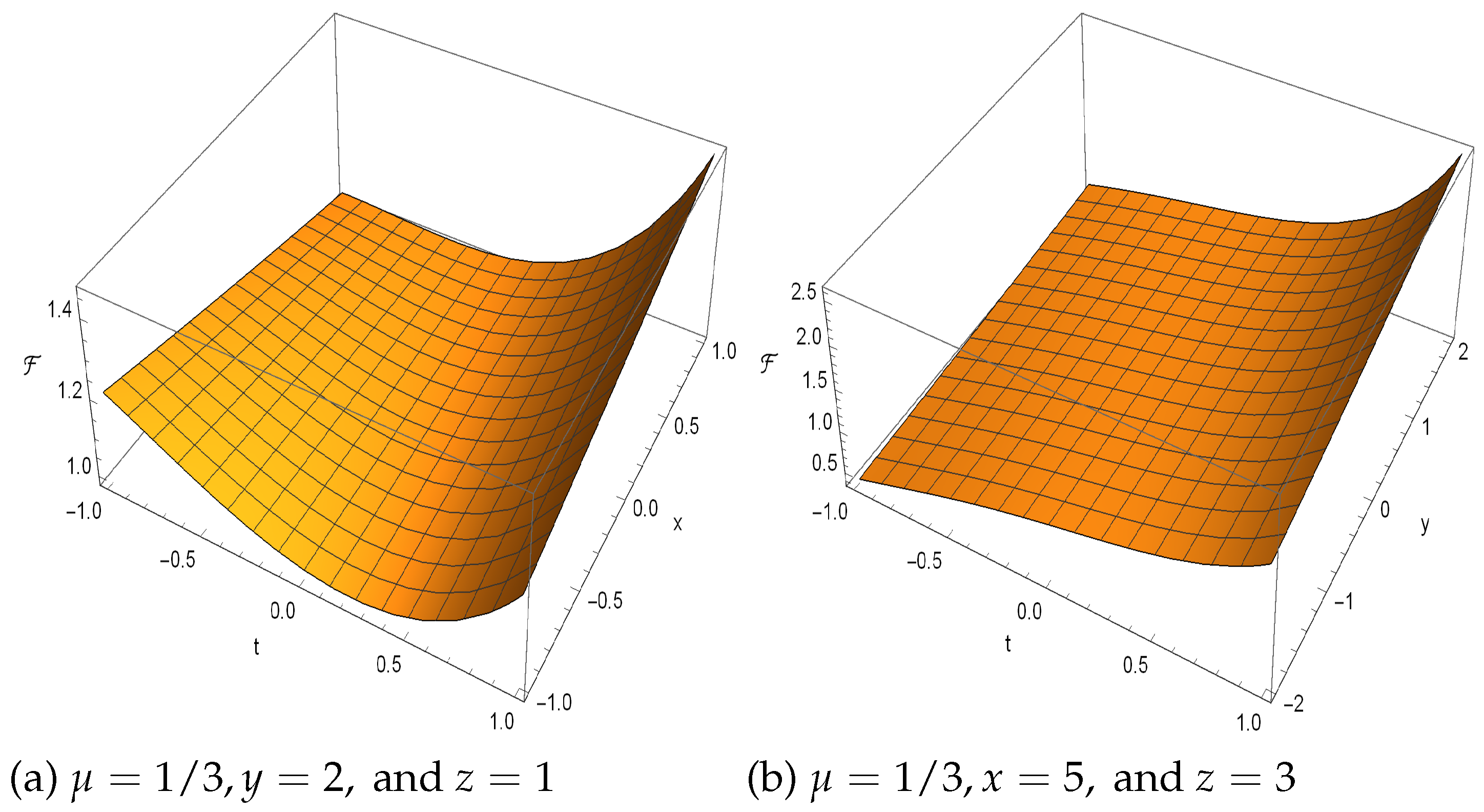
We have a picture of the surface for this solution.

In Figure 1a, we choose $-1\le x\le 1,-1\le t\le 1,\mu =1/3,$ and $y=2,z=1$. In Figure 1b, we choose $-2\le y\le 2,-1\le t\le 1,\mu =1/3,$ and $x=5,z=3$.

When we take N-th many derivative with respect to t for (4), we have

$${\left({\displaystyle \frac{\partial }{\partial t}}\right)}^N\mathfrak{F}(t,x,y,z|\mu )=\sum _{m=0}^{\infty }{\mathbf{H}}_{m+N}(x,y,z|\mu ){\displaystyle \frac{t^m}{m!}}.$$

(34)

From (19) and (34), we have the following theorem:

Theorem 9.

For $N=0,1,2,\dots$, one obtains

$${\mathbf{H}}_{m+N}(x,y,z|\mu )=\sum _{i=0}^m{\displaystyle \frac{{\mathbf{H}}_{m-i}(x,y,z|\mu )a_i(N,x,y,z|\mu )m!}{(m-i)!}}.$$

(35)

From (35) with $m=0$ one obtains the following corollary:

Corollary 3.

For $N=0,1,2,\dots$, one obtains

$${\mathbf{H}}_N(x,y,z|\mu )=a_0(N,x,y,z|\mu ),$$

where

$$\begin{array}{c}{a}_0(N+1,x,y,z|\mu )=1,\hfill \\ a_0(N+1,x,y,z|\mu )=\sum _{i=0}^N{\left({\displaystyle \frac{xlog(1+\mu )}{\mu }}\right)}^i{a}_1(N-i,x,y,z|\mu )\hfill \\ +{\left({\displaystyle \frac{log(1+\mu )}{\mu }}\right)}^{N+1}{x}^{N+1}.\hfill \end{array}$$

The first 3-variable degenerate Hermite Kampé de Feŕiet polynomials read

$$\begin{array}{c}{\mathbf{H}}_0(x,y,z|\mu )=1,\hfill \\ {\mathbf{H}}_1(x,y,z|\mu )={\displaystyle \frac{xlog(1+\mu )}{\mu }},\hfill \\ {\mathbf{H}}_2(x,y,z|\mu )={\displaystyle \frac{x^2{(log(1+\mu ))}^2}{{\mu }^2}}+{\displaystyle \frac{2ylog(1+\mu )}{\mu }},\hfill \\ {\mathbf{H}}_3(x,y,z|\mu )={\displaystyle \frac{x^3{(log(1+\mu ))}^3}{{\mu }^3}}+{\displaystyle \frac{6xy{(log(1+\mu ))}^2}{{\mu }^2}}+{\displaystyle \frac{6z{(log(1+\mu ))}^2}{{\mu }^2}},\hfill \\ {\mathbf{H}}_4(x,y,z|\mu )={\displaystyle \frac{x^4{(log(1+\mu ))}^4}{{\mu }^4}}+{\displaystyle \frac{12x^{2}y{(log(1+\mu ))}^3}{{\mu }^3}}+{\displaystyle \frac{24xz{(log(1+\mu ))}^2}{{\mu }^2}}\hfill \\ +{\displaystyle \frac{12y^2{(log(1+\mu ))}^2}{{\mu }^2}},\hfill \\ {\mathbf{H}}_5(x,y,z|\mu )={\displaystyle \frac{x^5{(log(1+\mu ))}^5}{{\mu }^5}}+{\displaystyle \frac{20x^{3}y{(log(1+\mu ))}^4}{{\mu }^4}}+{\displaystyle \frac{60x^{2}z{(log(1+\mu ))}^3}{{\mu }^3}}\hfill \\ +{\displaystyle \frac{60x{y}^2{(log(1+\mu ))}^3}{{\mu }^3}}+{\displaystyle \frac{120yz{(log(1+\mu ))}^2}{{\mu }^2}}.\hfill \end{array}$$

4. Roots of the 3-Variable Degenerate Hermite Kampé de Fériet Equations

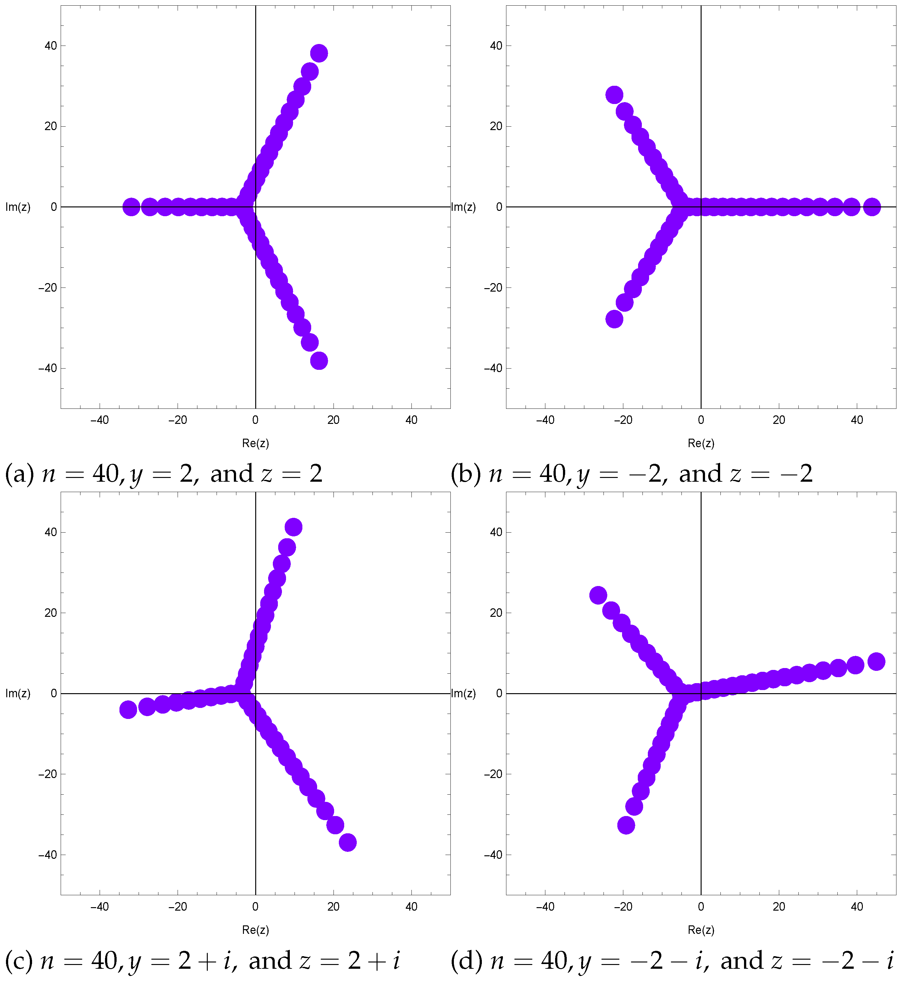
In this section we give a theoretical prediction via numerical experiments by finding a regular pattern for the roots of the 3-variable degenerate Hermite Kampé de Fériet equations ${\mathbf{H}}_n(x,y,z|\mu )=0$. To do this, we examine examples of several cases.

We look for the roots of ${\mathbf{H}}_n(x,y,z|\mu )=0$ for $n=40,y=2,-2,2+i,-2-i,z=2,-2,2+i,-2-i,\mu =1/3,$ and $x\in \mathbb{C}$ (Figure 2).

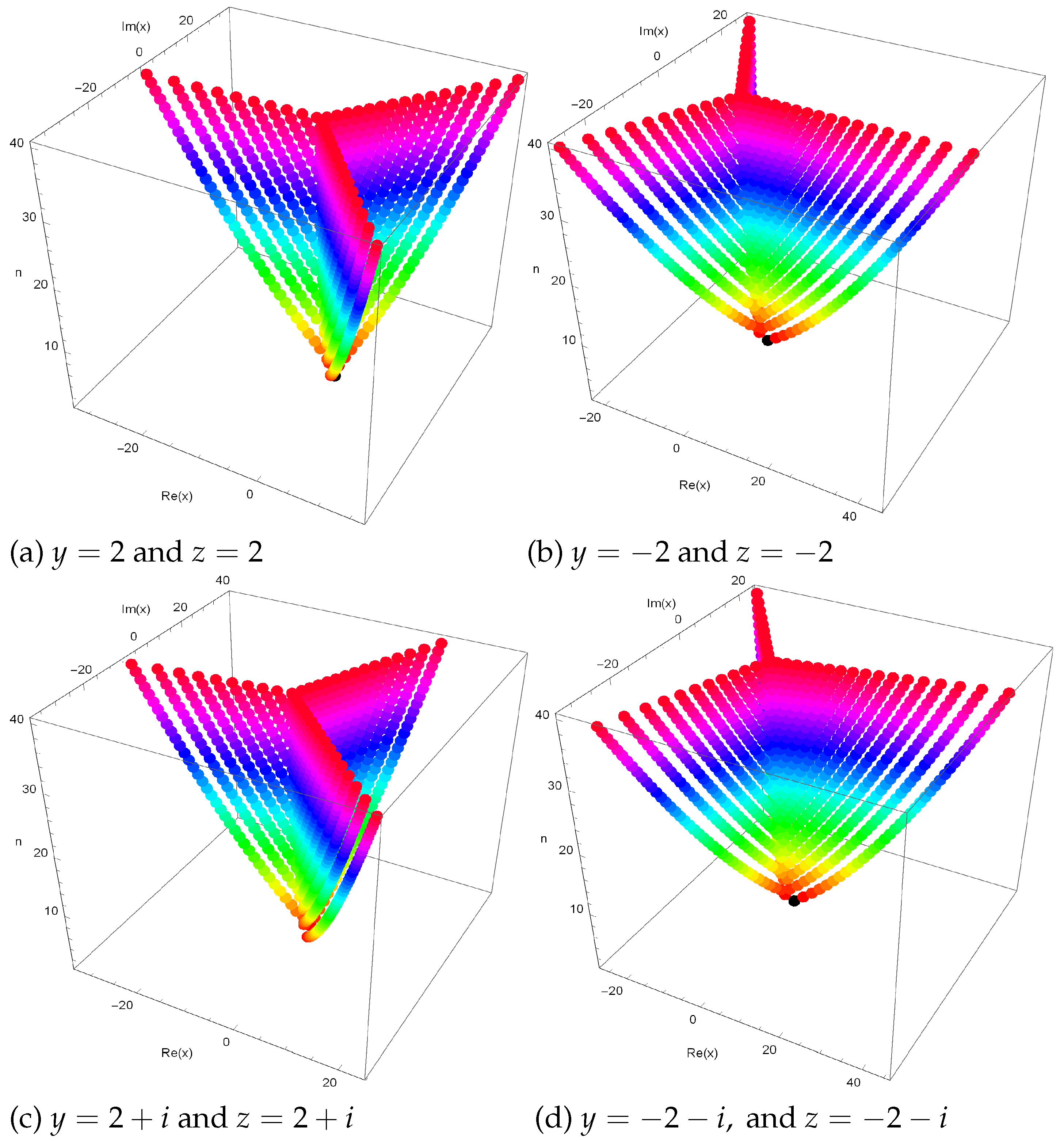
In Figure 2a, we select $n=40$, $y=2$, and $z=2$. In Figure 2b, we select $n=40$, $y=-2$, and $z=-2$. In Figure 2c, we select $n=40,$$y=2+i$, and $z=2+i$. In Figure 2d, we select $n=40$, $y=-2-i$, and $z=-2-i$. A picture of the roots of the 3-variable degenerate Hermite Kampé de Fériet equation ${\mathbf{H}}_n(x,y,z|\mu )=0$ for $1\le n\le 40,\mu =1/3$ from a 3-D structure are shown in Figure 3.

In Figure 3a, we select $y=2$ and $z=2$. In Figure 3b, we select $y=-2$ and $z=-2$. In Figure 3c, we select $y=2+i$ and $z=2+i$. In Figure 3d, we select $y=-2-i$ and $z=-2-i$. Our distributions for approximated solutions of real roots of equation ${\mathbf{H}}_n(x,y,z|\mu )=0$ are shown in

Table 1. Numbers of real and complex zeros of ${\mathbf{H}}_n(x,y,z|\mu )=0$.

Degree n	$\mathit{y}=2,\mathit{z}=2,\mathit{\mu }=1/3$		$\mathit{y}=-2-\mathit{i},\mathit{z}=-2-\mathit{i},\mathit{\mu }=1/3$
	Real Zeros	Complex Zeros	Real Zeros	Complex Zeros
1	1	0	1	0
2	0	2	0	2
3	1	2	0	3
4	0	4	0	4
5	1	4	0	5
6	2	4	0	6
7	1	6	0	7
8	2	6	0	8
9	1	8	0	9
10	2	8	0	10

and

Table 2. Approximate roots of ${\mathbf{H}}_n(x,y,z|\mu )=0,x\in \mathbb{C},y=2,z=2, \mathrm{and} \mu =1/3$.

Degree n	x
1	0
2	−2.1528 i,    2.1528 i
3	−1.0705,    0.5352 + 3.8424 i,    0.5352 − 3.8424 i
4	−1.1238 − 0.9119 i,    −1.1238 + 0.9119 i,    1.1238 + 5.4316 i
	1.1238 − 5.4316 i
5	−2.6937,    −0.3500 − 2.3168 i,    −0.3500 + 2.3168 i
	1.6969 + 6.9000 i,    1.6969 − 6.9000 i
6	−3.6974,    −1.1016,    0.1447 − 3.6924 i
	0.1447 + 3.6924 i,    2.2548 + 8.2725 i,    2.2548 − 8.2725 i
7	−4.8260,    −1.0340 + 1.3912 i,    −1.0340 − 1.3912 i,    0.6498 + 4.9794 i
	0.6498 − 4.9794 i,    2.7972 − 9.5687 i,    2.7972 + 9.5687 i

.

We can observe a regular pattern of the complex roots of the 3-variable degenerate Hermite Kampé de Fériet equation ${\mathbf{H}}_n(x,y,z|\mu )=0$. We hope to prove regular pattern of the complex roots of the 3-variable degenerate Hermite Kampé de Fériet equations ${\mathbf{H}}_n(x,y,z|\mu )=0$ (Table 1).

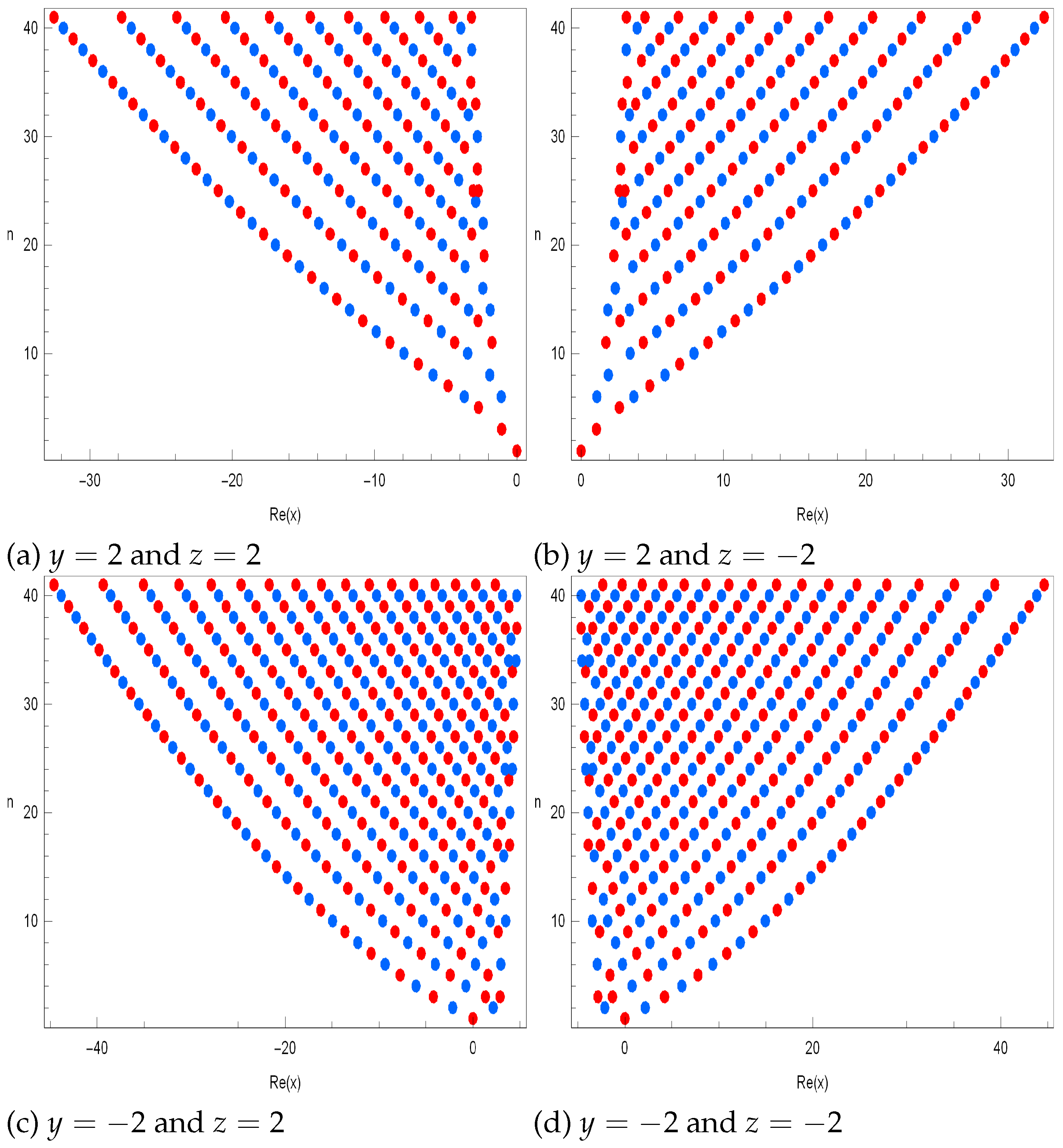
A picture of real roots of equations ${\mathbf{H}}_n(x,y,z|\mu )=0$ for $1\le n\le 40,\mu =1/3$ are displayed in Figure 4.

In Figure 4a, we select $y=2$ and $z=2$. In Figure 4b, we select $y=2$ and $z=-2$. In Figure 4c, we select $y=-2$ and $z=2$. In Figure 4d, we select $y=-2$ and $z=-2$.

Next, we obtain an approximate solution satisfying ${\mathbf{H}}_n(x,y,z|\mu )=0,x\in \mathbb{C}$ for given $n,y=2,z=2$, and $\mu =1/3$ in the Table 2.

5. Conclusions and Future Directions

In this article, we constructed the 3-variable degenerate Hermite Kampé de Fériet polynomials and got symmetric identities for 3-variable degenerate Hermite Kampé de Fériet polynomials. We also made the differential equations which are related to the generating function of ${\mathbf{H}}_n(x,y,z|\mu )$. We also studied the symmetry of pattern of the roots of the 3-variable degenerate Hermite Kampé de Fériet equations ${\mathbf{H}}_n(x,y,z|\mu )=0$ for various variables $x,y,$ and z. As a result, we found that the distribution of the roots of 3-variable degenerate Hermite Kampé de Fériet equations ${\mathbf{H}}_n(x,y,z|\mu )=0$ has regular pattern. So, we make the following series of conjectures with numerical experiments:

We use some notations. $R_{{\mathbf{H}}_n(x,y,z|\mu )}$ denotes the number of real zeros of ${\mathbf{H}}_n(x,y,z|\mu )=0$ on the real plane, that is, $Im\left(x\right)=0$, and $C_{{\mathbf{H}}_n(x,y,z|\mu )}$ denotes the number of complex zeros of ${\mathbf{H}}_n(x,y,z|\mu )=0$. Since n is the degree of the polynomial ${\mathbf{H}}_n(x,y,z|\mu )$, we obtaine $R_{{\mathbf{H}}_n(x,y,z|\mu )}=n-C_{{\mathbf{H}}_n(x,y,z|\mu )}$.

We can see a regular pattern of the complex roots of the 3-variable degenerate Hermite Kampé de Fériet equations ${\mathbf{H}}_n(x,y,z|\mu )=0$ for $y,z$, and $\mu$. Therefore, we can make thebelow conjecture.

Conjecture 1.

Let $n=2,3,\dots ,$ and $y\in \mathbb{C}$. Prove or disprove that

$$R_{{\mathbf{H}}_n(x,y,z|\mu )}=0,C_{{\mathbf{H}}_n(x,y,z|\mu )}=n,$$

where $\mathbb{C}$ is the set of complex numbers.

Conjecture 2.

For $n=2,3,\dots ,$ and $z\in \mathbb{C}$, prove or disprove that

$$R_{{\mathbf{H}}_n(x,y,z|\mu )}=0,C_{{\mathbf{H}}_n(x,y,z|\mu )}=n.$$

The Conjectures 1 and 2 are unsolved problems for all variables $y,z$ and $\mu$.

We see that the solutions of the 3-variable degenerate Hermite Kampé de Fériet equations ${\mathbf{H}}_n(x,y,z|\mu )=0$ does not show reflection symmetry about $Re\left(x\right)=a$ for $a\in \mathbb{R}$ (see Figure 2, Figure 3 and Figure 4).

Conjecture 3.

Prove that ${\mathbf{H}}_n(x,y,z|\mu ),x\in \mathbb{C},y,z\in \mathbb{R}$ as an analytic complex function has reflection symmetry $Im\left(x\right)=0$.

Finally, we consider the more general problems. How many roots does ${\mathbf{H}}_n(x,y,z|\mu )=0$ have? We are not able to decide whether ${\mathbf{H}}_n(x,y,z|\mu )=0$ has n distinct solutions. We would like to know the number of complex roots $C_{{\mathbf{H}}_n(x,y,z|\mu )}$ of ${\mathbf{H}}_n(x,y,z|\mu )=0.$

Conjecture 4.

Prove or disprove that ${\mathbf{H}}_n(x,y,z|\mu )=0$ has n distinct solutions.

The conjecture 4 is unsolved problem for all variables n (see Table 1 and Table 2).

If we can theoretically prove the above problems by drawing new ideas from various numerical results, we look forward to contributing to research related to the 3-variable degenerate Hermite Kampé de Fériet equations ${\mathbf{H}}_n(x,y,z|\mu )=0$ in applied mathematics, mathematical physics, and engineering.

References

Andrews, L.C. Special Functions for Engineers and Mathematicians; Macmillan. Co.: New York, NY, USA, 1985. [Google Scholar]
Appell, P.; de Fériet, J.H.K. Fonctions Hypergéométriques et Hypersphériques: Polynomes d Hermite; Gauthier-Villars: Paris, France, 1926. [Google Scholar]
Dattoli, G. Generalized Polynomials Operational Identities and Their Applications. J. Comput. Appl. Math.2000, 118, 111–123. [Google Scholar] [CrossRef] [Green Version]
Erdelyi, A.; Magnus, W.; Oberhettinger, F.; Tricomi, F.G. Higher Transcendental Functions; Krieger: New York, NY, USA, 1981; Volume 3. [Google Scholar]
Andrews, G.E.; Askey, R.; Roy, R. Special Functions; Cambridge University Press: Cambridge, UK, 1999. [Google Scholar]
Arfken, G. Mathematical Methods for Physicists, 3rd ed.; Academic Press: Orlando, FL, USA, 1985. [Google Scholar]
Khan, S.; Yasmin, G.; Khan, R.; Hassan, N.A.M. Hermite-based Appell polynomials: Properties and applications. J. Math. Anal. Appl.2009, 351, 756–764. [Google Scholar] [CrossRef] [Green Version]
Carlitz, L. Degenerate Stiling, Bernoulli and Eulerian numbers. Utilitas Math.1979, 15, 51–88. [Google Scholar]
Young, P.T. Degenerate Bernoulli polynomials, generalized factorial sums, and their applications. J. Number Theorey2008, 128, 738–758. [Google Scholar] [CrossRef] [Green Version]
Cenkci, M.; Howard, F.T. Notes on degenerate numbers. Discrete Math.2007, 307, 2375–2395. [Google Scholar] [CrossRef]
Ryoo, C.S. Notes on degenerate tangent polynomials. Glob. J. Pure Appl. Math.2015, 11, 3631–3637. [Google Scholar]
Haroon, H.; Khan, W.A. Degenerate Bernoulli numbers and polynomials associated with degenerate Hermite polynomials. Commun. Korean Math. Soc.2018, 33, 651–669. [Google Scholar]
Hwang, K.W.; Ryoo, C.S. Some identities involving two-variable partially degenerate Hermite polynomials induced from differential equations and structure of their roots. Mathematics2020, 8, 632. [Google Scholar] [CrossRef] [Green Version]
Kim, T.; Kim, D.S.; Kwon, H.I.; Ryoo, C.S. Differential equations associated with Mahler and Sheffer-Mahler polynomials. Nonlinear Funct. Anal. Appl.2019, 24, 453–462. [Google Scholar]
Ryoo, C.S. A numerical investigation on the structure of the zeros of the degenerate Euler-tangent mixed-type polynomials. J. Nonlinear Sci. Appl.2017, 10, 4474–4484. [Google Scholar] [CrossRef] [Green Version]
Ryoo, C.S. Differential equations associated with tangent numbers. J. Appl. Math. Inform.2016, 34, 487–494. [Google Scholar] [CrossRef]
Ryoo, C.S. Some identities involving Hermitt Kampé de Fériet polynomials arising from differential equations and location of their zeros. Mathematics2019, 7, 23. [Google Scholar] [CrossRef] [Green Version]
Ryoo, C.S.; Agarwal, R.P.; Kang, J.Y. Differential equations associated with Bell-Carlitz polynomials and their zeros. Neural Parallel Sci. Comput.2016, 24, 453–462. [Google Scholar]
Figure 1.
The surface for the solution .
Figure 2.
Zeros of .
Figure 3.
Stacks of zeros of .