Modelling of Consumption Shares for Small Wind Energy Prosumers

Abstract

This article describes a simulation of energy distribution in an average household where electricity is produced with a small wind generator or purchased from the public electricity grid. Numerical experiments conducted within an average of five minutes were performed using annual production and consumption graphs. Virtual storage devices, a water tank and a battery were used to buffer energy inside the household. The energy required for non-shiftable consumption and hot water consumption were taken directly from the utility grid. Surplus energy remaining from wind generator production after providing for consumption and storage needs were redirected there. A cover factor was used as a measure of the efficiency of energy distribution. One of the aims of the article was to determine by simulations the change of the cover factor in a virtually designed situation where the expected energy output of the wind generator was known in advance over one to three hours. The results found that for the configuration of the proposed nanogrid option, the positive results were readily achieved when the expected wind generator production was known an hour ahead. Then, the cover factor increased from 0.593 to 0.645. The side result of using projected/expected production is an increase in asymmetrical energy exchanges bilaterally between nanogrid and utility grid in favour of grid sales. Another finding was that the cover factor depended on the wind generator’s production intensity but less on the intensity of consumption within the household.It is hoped/expected that future research will address the prediction of output using mathematical methods.

1. Introduction

Across the globe, renewable energy systems are being supported and applied as replacements to traditional energy resources. The European Union’s energy policy plans to create 32% of power generation from renewable resources by 2030 [1]. Therefore, rising consideration is being offered to transforming energy from similar renewable resources, particularly solar, geothermal and wind [2]. However, these natural energy sources present challenges to electrical engineers and researchers on the mode of optimising energy extractions for on-site use, and its deployment as alternative to fossil energy sources [3,4].

It is known that increasing or having a high share of self-consumption with wind generator equipped or/and PV panels prosumers have a significant influence on the state-of-art public utility grid. The energy that we produce on-site does not load the public grid but sometimes feeds it. If we produce and consume energy on-site, we need less reinforcement of the utility grid. The losses in the utility grid are lesser when we consume more energy on-site. Nevertheless, it is relevant to maintain enough rotating reserve in terms of national energy security, which helps keep the electricity grid’s stability [5,6].

This paper presents a computer simulation of electrical energy distribution management in a typical Estonian household in Europe. Energy is produced by a wind generator (WG) or purchased from the public utility grid (UG). All consumption is divided into two parts: Consumption via non-shiftable equipment and heated water consumption. Essential parts of the simulation system are in-house energy storage devices, i.e., the water tank and battery. The main task of energy storage management is to maximise the cover factor as the MATLAB simulations’ main evaluation parameter. Cover factor videlicet demand cover factor (Y_D) expresses the share of self-consumption of wind energy in the nanogrid using renewable energy sources. For a given time series of averaged over five minutes of consumption and production data, optimal battery and water tank sizes were derived. One objective was to increase the cover factor through a more advanced configuration of an in-house equipment system.

Besides, efforts were made to increase the value of cover factor and, by extension, load control efficiency by using the wind turbine’s expected production, measured within one to three hours in advance. The wind generator’s production pattern is very stochastic in that it has a random probability pattern and thus, may not be precisely predicted to give the desired results. The study showed that advance information about expected production could increase the cover factor. The time series of the given raw data was treated as a prediction. The energy management was altered according to whether more or less production volume was expected than the current sample period. In conclusion, it is safe to say that forecasting production volume has a positive effect on self-consumption. It is expected that this approach adopted for nanogrid design and control is transferable to other systems such as industrial, commercial, and apartment buildings.

This article is structured as follows: Section 2 gives a short overview of scientific papers where similar problems are reviewed. Section 3 describes the configuration of the modelled household. In Section 4, there is a discussion of the initial data and input parameters used in simulation experiments. Section 5 describes the simulation setup and presents the main simulation algorithm. In Section 6, the primary indicator of energy flow distribution efficiency—cover factor—is introduced. The results are divided into three groups, which are reviewed in successive sections. According to the given configuration, the usable water heater (WH) and battery capacity and the cover factor are presented in the following sections. Section 7 discusses the factors that affect the cover factor with different values of amplification coefficient and deterministic expected production. Coefficient R_S of wind generator production was used to express the annual output energy’s amount concerning consumption. Finally, Section 8 compares energy exchanges between nanogrid and utility grid, with and without considering the deterministic expected production. Problems for discussion are in Section 9, while conclusions are in Section 10.

2. Overview of Literature

A review of the literature indicates that relatively little attention has been given to investigating the potential for increasing the cover factor.

Overall, the demand cover factor Y_D expresses the locally produced share and thereby directly consumed renewable energy to annual total consumption. In scientific literature, the cover factor is often described by the term self-consumption. The source of renewable energy in this article is wind.

Some researchers referenced it as the (LMI) or (LGMI) [7,8]. For instance, the thematic review article [9] described distributed energy from minimising energy losses, optimising energy quality and reducing the cost of such losses. The article’s [10] main goal was to decrease operational losses when storing batteries’ energy. Vanhoudt et al. [11] explored the possibility of deploying a heat pump to increase self-consumption, which is indirectly related to energy storage. They compared the sources of electricity and found that wind energy provides a higher share of self-consumption than solar PV. However, the problem was the drop in the heat pump’s temperature during calm periods, which caused additional energy losses. Naval et al. [2] modelled the issues of diversity of energy sources and the related problems of monitoring electricity price. The wind was one of the potential energy sources in that experiment. Researchers often study the effects of combining solar PV and wind energy production on a microgrid operation [12,13]. Increasing self-consumption stabilises load peaks and decreases costs on the electrical energy purchase [14]. Other research studies with a similar objective as this study, but based on solar PV, are described in the references [11,12], while cross-seasonal storage is discussed in others [15,16]. The latter demonstrates the possibility of increasing self-consumption by incorporating space heating demand and using large volumes of water and concrete to store energy. HOMER Pro software was employed to model net-zero energy (NZE) hybrid microgrid with battery energy storage system (BESS), combined with a wind generator and PV panels [17]. It was found that at a moderate cost of electricity, on-grid NZE was the optimal solution without BESS. However, HOMER Pro software was not used as it does not allow the processing of data for shorter periods than one hour.

Load shifting technology was designed to cope with stochastic production patterns of energy sources, especially wind and solar [18,19,20,21,22]. This technology allows the increase in self-consumption by using storage devices —the wind’s inland speed changes on a random schedule. Except there are cyclones located close to larger water bodies, wind speed changes indicate a definite 24 h pattern of occurrence. In addition to high stochasticity, other problems associated with wind-generated production include occasional storm and calm periods, which can be reasonably long. Solar energy is only available at noon in the summer when production is optimal and consumption is low. If both wind and solar PV production equipment are used, their balancing effect positively impacts the increase in self-consumption. By adopting a solution where the ratio of annual wind and solar PV production is 30%/70% favouring wind energy, it is possible to increase the share of renewable energy cover factor in total consumption up to 0.6 [23]. Eltanay et al. [24] incorporated load prioritisation in addition to load shifting technology and divided loads into two groups. In [25,26], the authors employed the methodology to derive the size of a battery energy storage system (BESS) for self-consumption optimally in windless times, and operated the BESS to maximise its technical and economic benefits. Distributed energy resources for households should consist of as many energy sources as possible [2,27] to improve economic parameters. With the addition of the storage device, the self-consumption of wind energy increased by almost 10% [27]. In Spain, different energy generation systems based on solar PV are competitive and profitable without subsidies in self-consumption schemes [28]. In fact, the setting up of distributed generation, when exploited in a self-sufficiency manner, may decrease the utilisation peaks [29]. Scientists and experts demonstrated that this kind of arrangement might enhance a microgrid’s resilience and improve the level of self-consumption whilst decreasing the grid loads, which means being cost-effective up to 60% of self-consumption [30].

In this work a simple yet accurate method has been proposed in nanogrids to find a cover factor using WG’s expected production that mimics the wind speed forecast from the weather service. The wind speed forecast is then converted to WG’s hourly average output power. It was assumed that the electric grid is operating as intended, and the stability issues have been excluded from the analysis. For example, the study in [30] describes large signal stability of an inverter-based generator using a Lyapunov function; in [31], the work is related to microgrids decentralised and hierarchical control, and in [32], the study provides as a new model of a converter-based generator. These topics are an important aspect in the implementation of such systems, however, in this investigation, only the energy flows between the renewable generator, the storage equipment, consumers and UG are examined, while the stability issues associated with the operation of inverters are out of scope of this paper.

Small cogeneration heat plants (CHP) powered by biofuels can support grid stability to some extent, but burning biofuels is harmful to the environment and, thus, not ideal [33]. Furthermore, CHPs have a thermal energy component that limits their size and broader use. Hydropower is environmentally friendly and stable in 24 h cycles but seasonally variable [34,35]. Pump hydroelectric power plants can be used for large-scale electricity storage [36]. Due to the absence of significant hydropower resources in Estonia, this area is not the focus of the present study. Flywheel storage [37] is also used as a storage device in smart grids, for transport and for maintaining grid stability, but in recent times, supercapacitors have started to replace them. Moreover, flywheels can be used only for short-term storage, not for days or even hours.

3. Technical Configuration of Nanogrid

The term nanogrid (NG) refers to an electrical installation, which comprises local electricity generation, loads, storage and utility grid connection by default [38].

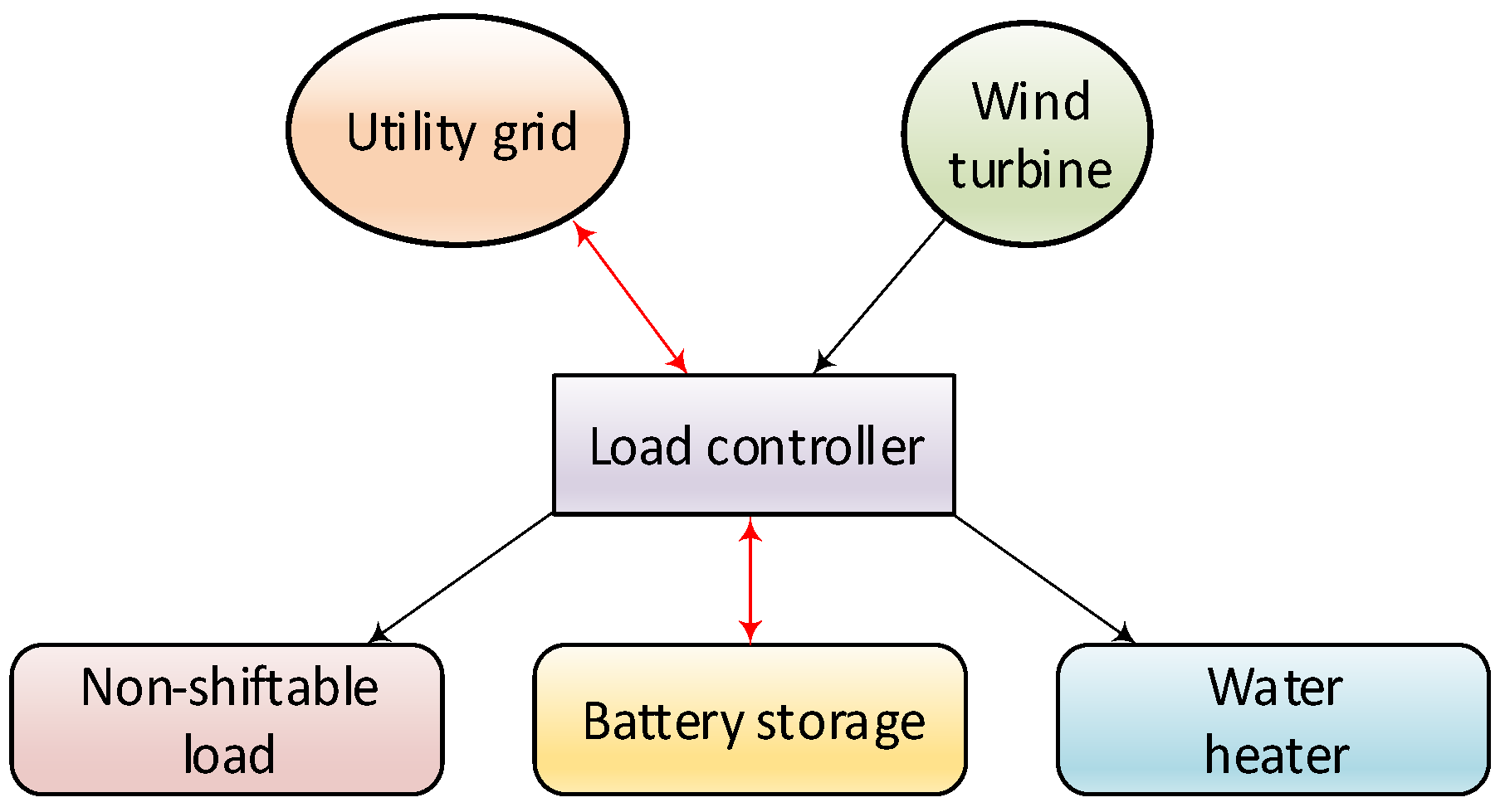
A wind generator powers the private house nanogrid. Figure 1 shows the technical configuration and flow diagram, which describes the energy moving principles inside the household or nanogrid (NG). The main components of the system are wind generator (WG), non-shiftable energy consumption equipment (NS), water heater (WH) and storage battery (SB). Locally installed WG is considered a renewable energy source. In every sample interval (see below), the generator’s energy production surplus is directed to the utility grid (UG). The deficit of internal consumption is compensated by the energy purchased from the UG. The energy consumers in the NG are ordinary household electrical appliances such as lighting, air conditioning, television sets, kitchen appliances, washing machine with dryer, stove, refrigerator, and electronic equipment, etc., so-called non-shiftable energy load equipment. Water heaters are considered separate equipment. The residential prosumer has a stationary SB storage system for the case of energy excess or deficit. There is an SB and a WH because the wind energy production does not match the residential continuous demand profile and there is an urgent need to store energy during high production/supply periods and need energy over the low generation periods.

The numerical simulation presents the operation of the load controller, the central element of NG. Numerical experiments aim to find the values of technical parameters of NG components. The most appropriate values for these parameters are proposed based on expert judgment. The best mathematical approach would require setting up an optimisation problem, which is our next task. This requires the introduction of an economic optimisation environment with appropriate objective function and constraints.

4. Dataset Parameters and Description

By means of input data, a time series of a generation of the WG is normalised to rated power P_nom = 5 kW, produced by TUGE Ltd. (TUGE Ltd., Paldiski, Estonia) [39] was employed. This later is mounted in an offshore region per coordinates N 59.087694, E 23.591719. The assembled data package includes the time from 1 December 2015 to 30 November 2016, considering that December is the initial winter month, enabling further seasonal evaluation. The mean WG power output is calculated by dividing the electricity produced over the latest sampling epoch by the interval of the sample epoch Δt. In the current study, Δt = 5 min, and a year are split into periods of 5 min in span. Generation and loads are sampled in the same manner. The yearly production of the WG is normalised to equal the annual load as close as feasible.

An archetypal individual residential’ s load profile is examined with NS load and hot water production (B) elements. The overall logged yearly electricity utilisation was 3473 kWh, among which 47% (1632 kWh) was billed to NS (white goods, TV-set, lighting, etc.) and 53% (1841 kWh) to B, according to actual measured values [40]. SB and WH capacities are deemed usable net values. Energy-associated factors, for instance, WH temperatures, are not evaluated and nor is the energy required to attain WH minimal temperature of 55 °C, to prevent reproducing Legionella bacteria [41]. Operating temperature is presumed to have been reached.

We are looking for minimal WH and SB sizes in simulations that give a proportional maximum effect to increase the cover factor (see Section 7). For the electrical energy storage elements, we assume the use of lead-acid deep cycle batteries Victron Energy BAT412123081239 Ah [42], or similar.

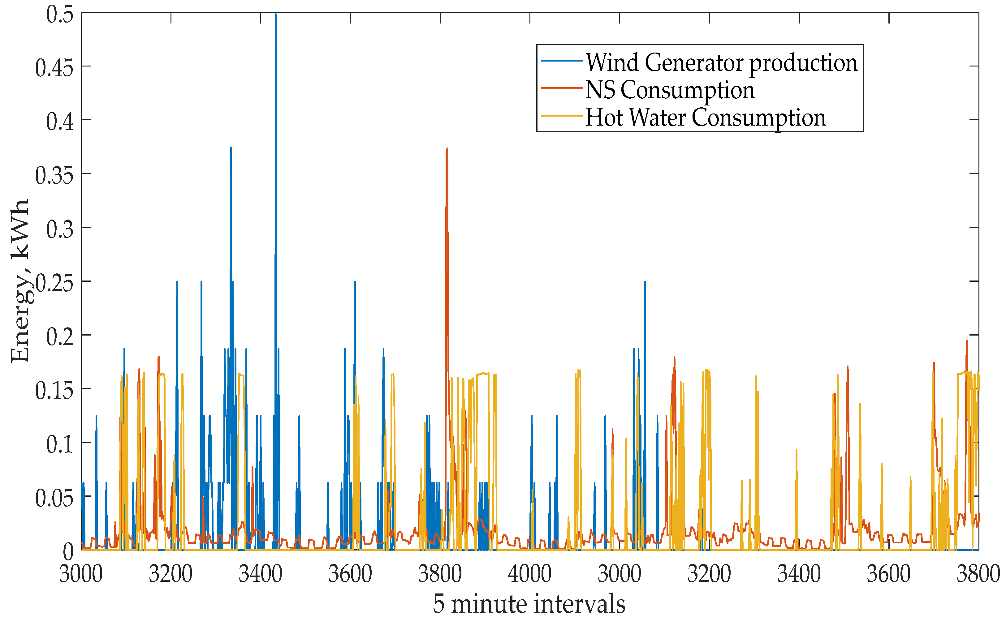
Figure 2 shows an example of energy data as a function of time in 5 min intervals. The total length of the time series is 105120; on this figure, a choice of 1000 intervals is depicted.

5. Simulation Algorithm

Next, we introduce the load control simulation algorithm. The easiest way is to describe it by pseudo-code, a plain language description of the algorithm’s steps. In this code, we use notations, which were explained in Section 4. Algorithm 1 presents the algorithm for calculating the maximum cover factor. The sharing algorithm in every time interval is outlined in Algorithm 1 below [43].

Algorithm 1. Determining the Maximum Cover Factor
1.	START load initial data time series and necessary parameter values
2.	Create data structures and spaces
3.	INIT initialise next sample 5 min interval
4.	FOR1 every sample interval
5.	INPUT read data sample values from the data time series
6.	Transfer energy residues from the previous periods
7.	FOR2 every fixed value of storage equipment capacity
8.	IF1QNS < QWG
9.	Satisfy NS consumption
10.	IF2 Pnow > Pexp
11.	Fill SB
12.	Fill WH
13.	Satisfy the need for water heating from WH, SB or UG
14.	ELSE2 fill WH.
15.	Satisfy the need for water heating from WH, SB or UG
16.	Fill SB
17.	ENDIF2
18.	ELSE1 take missing part for NS consumption from SB or UG
19.	Satisfy the need for water heating from WH, SB or UG
20.	ENDIF1
21.	ENDFOR2
22.	Save results
23.	ENDFOR1
24.	Compute cover factor
25.	Plots and printouts
26.	STOP

where:

P_now is the WG capacity in the current time interval hour (kW);

P_exp is the expected capacity of WG one or more hours ahead (kW);

Q_WG is the energy production of WG in the current time interval (kWh);

Q_NS is the non-shiftable energy consumption in the current time interval, energy (kWh).

A wind generator powers the private house nanogrid. The algorithm from Algorithm 1 describes the simulation process. The total quantities of electricity produced and consumed during a year are nearly equal. At first, the NS consumption demand is satisfied. In the case of WG production surplus, the energy is distributed according to the current time interval situation. The power generated from WG should be used either for storing in the SB or meeting the load demand of WH. Buying from the grid should be avoided as much as possible to achieve the cheapest scheduling. However, it may be seen that the SB is full at some hours, and the WG production is more significant than load demand. Installing a SB with low energy capacity or small consumption of the system compared with generated power from WG can lead to the need for purchasing the energy from UG.

If the deterministically available expected value taken n hours ahead from the present moment, i.e., the wind generator’s capacity shortly is less than the energy production amount on instant time, P_now > P_exp. The wind generator output first satisfies non-shiftable loads (NS), then the SB until it is not fully charged and then the boiler. Considering the energy deficit soon, after n hours, the SB will be prioritised after the NS load has been met. In this case, the SB powers both the NS and the WH according to the B consumption schedule. We used the values of n = 1, 2, 3, 4 and 5 in simulations.

If n hours ahead, the expected production value is greater than the current moment value, P_now < P_exp, the wind generator output first satisfies NS loads. The energy moves to the WH, which also meets the B needs. After B consumption, the WH is refilled with as much energy as is left from the NS. If the process does not require all the energy, the excess will move to the SB, and if there is more energy left, it will go to the utility grid. If the WG output is missing or the NS is partially satisfied, the missing energy is taken from the SB or, if there is still a deficit, from the utility grid.

This approach provides a better chance of recharging control of the battery when the energy deficit is foreseen. However, it must be considered that consumption from WH is also based on the consumption schedule B. WH functions as a boiler, from which heated water is taken for hot water needs.

6. Cover Factor, Storage Battery (SB) and Water Heater (WH) Size Selections

To achieve the objectives of this article, we performed a computer simulation. All devices of the household’s energy system (Figure 1) were represented as components of the simulation scheme that can be linearly loaded or unloaded with energy. Three time series were used as inputs: annual energy production of the wind generator, the yearly demand of non-shiftable energy consumption devices considered altogether, and energy consumption through all hot water taps. Time series were pre-processed after the collection of raw data and averaged at five-minute intervals over one year. Every time series has 105,120 elements.

To estimate the concurrence level between generation and consumption, Baetens et al. [44] recommended the utilisation of two cover factors. The supply cover factor Y_S is termed as the ratio to which the energy demand covers the area supply; the demand cover factor Y_D is the ratio to which the energy demand is covered by the area supply. We use in our simulations only Y_D what describes the share of renewables in the consumption. We use the cover factor formula from Baetens et al. [44], which in our case study is interpreted in the form:

$$Y_D=\frac{W_{NS\ast }+W_{WH}+W_{Bat}}{W_{NS}+W_B}$$

(1)

where:

$W_{NS\ast }$ is the total annual amount of energy produced by a wind generator, which is directly consumed by non-shiftable devices needs;

$W_{WH}$ is the sum of energy from WG that is used with hot water consumption from WH during the year;

$W_{Bat}$ is the sum of energy that is used in case of lack of energy for non-shiftable consumption from SB annually;

$W_{NS}$ is the total energy needed in NS load during the year;

$W_B$ is the amount of energy representing the total energy consumed for water heating during the year.

The demand cover factor Y_D (Equation (1)) shows the ratio in which the energy demand is covered by the local supply and characterises the self-satisfaction of the household [11]. The simulation is arranged as shown on the flow chart in Figure 1 and Algorithm 1. The detailed approach is described in Section 5. Using expected production then asymmetrical energy exchange between nanogrid and utility grid appears. To relieve this, we also examine situations where we increase or decrease annual wind energy production and see how this affects the cover factor and energy exchange between nanogrid and utility grid.

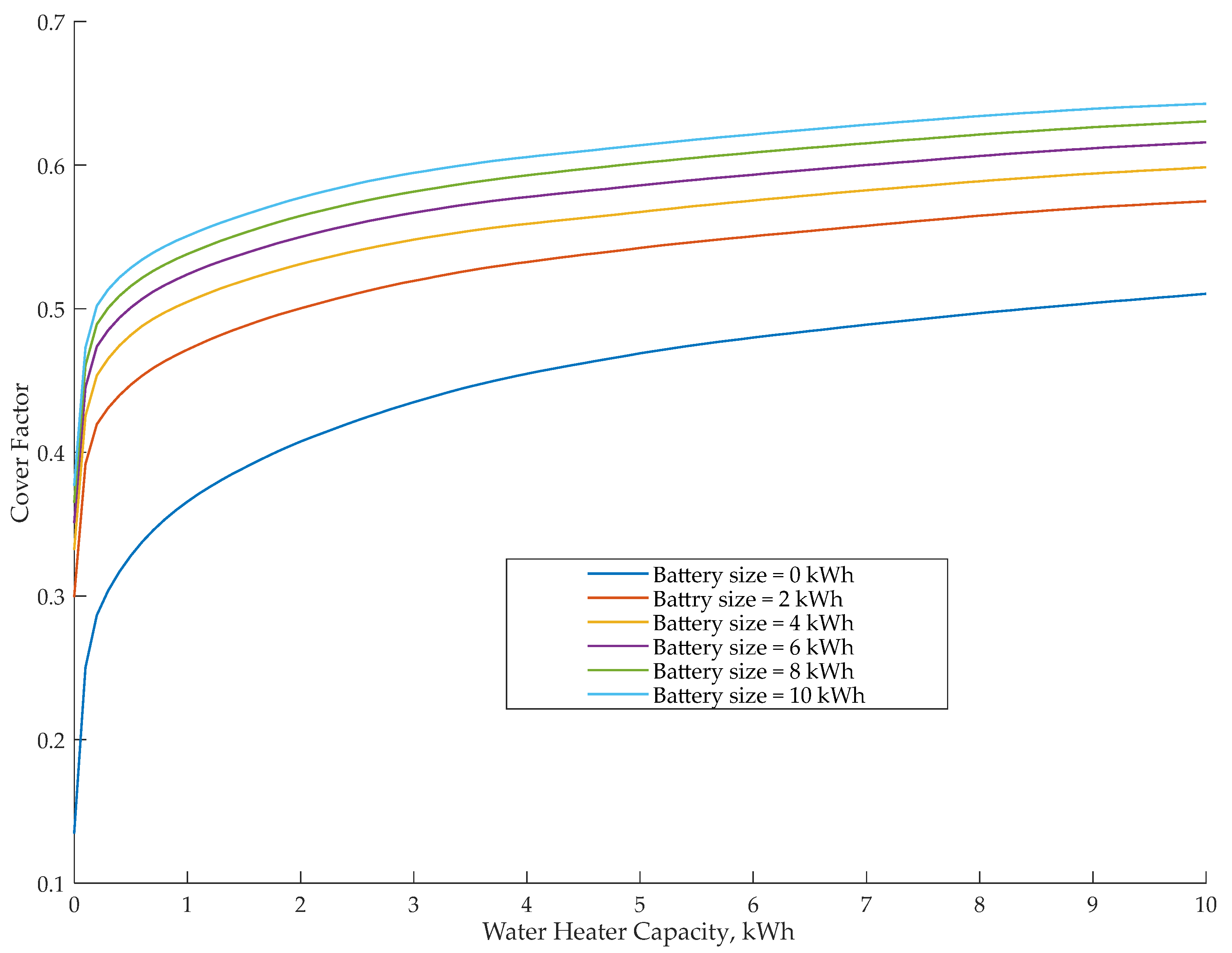
In Figure 3, we see the cover factor Y_D dependency on SB and WH capacity. At first, some values of maximum possible capacities of SB are fixed. Then, for every maximum capacity size, the cover factor’s value is calculated as a function of the maximum size of WH. The last changes in the interval [0,10] with the unit step. Six different graphs of these functions are presented SB capacities 0, 2, 4, 6, 8 and 10 kWh. We see an increase in cover factor depending on the growth of SB size. It can be observed that after 6 kWh of SB, the increase of cover factor becomes more pronounced. Therefore, based on literature and expert judgment, the 6 kWh value was selected for the following analysis. We choose 6 kWh as appropriate water heater and SB capacity values for the next simulation stages because the increase of cover factor for higher values is slowing. An important criterion of selection was the minimal size in maximum effectiveness. WH size is selected a little larger than on scheduled water consumption of one day. Choosing SB capacity, the criteria “small as possible” and “large as needed” were considered. We assume that the lowest needed working temperature in WH is already achieved. For the SB capacity, we mean the capacity between the maximum discharge and fully charged condition.

Figure 3 illustrates the sensitivity of the cover factor to the maximum capacity values of WH and SB. To get this drawing, 660 simulations were performed, one for every node point, i.e., fixed pair (WH_max, Bat_max) of WH maximum capacities WH_max from 0 to 10 with step size 0.1 and of six values of SB sizes Bat_max.

7. Improvement of Cover Factor Using Wind Generator Expected Production

We proposed and applied relevant novel cover factors in this work to assess the efficiency and differentiate diverse nanogrid arrangements and energy flow in the above-listed. In the literature, one can find numerous types of cover factors. In our numerical simulations, Equation (1) for this was used.

Shortly, the cover factor is the ratio of energy produced by the wind generator, consumed in the household under consideration. It is easy to see that the following inequalities hold:

0 ≤ Y_D ≤ 1,

(2)

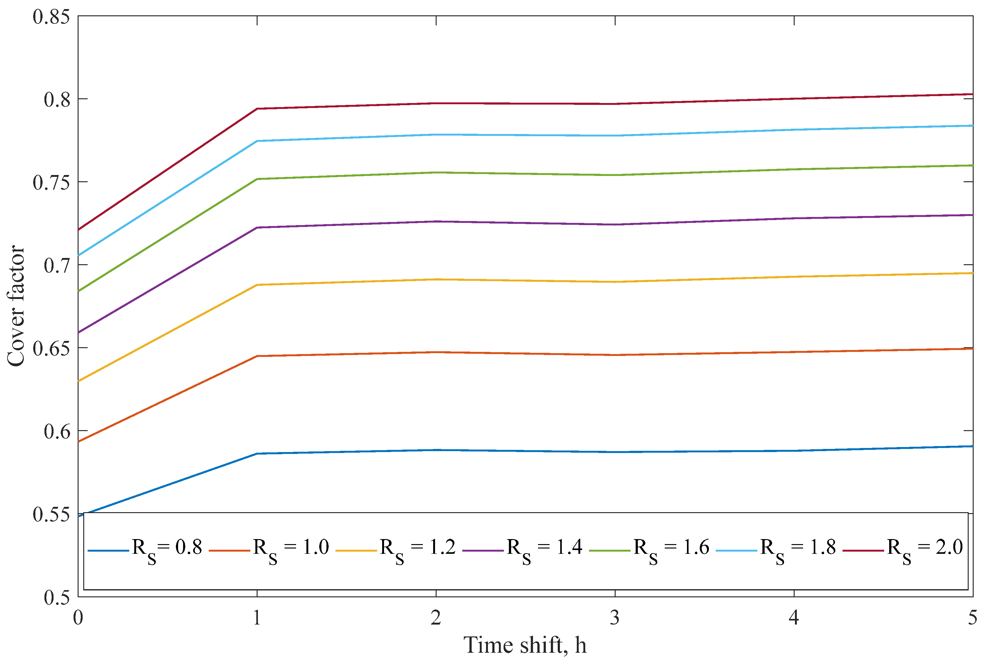
The prosumer’s goal when installing the equipment in nanogrid and WG is to maximise the cover factor. Parameter Y_D serves as a quantitative indicator of the efficiency of the household energy system. Figure 4 shows the impact of the expected production P_exp on cover factor Y_D after the WG production energy output is amplified by different coefficient R_S. We considered that R_S is a ratio of the energy produced by WG to consumption. In Section 5, we saw that the energy flow control system reacts to the comparison of energy production amount in current time, P_now, and the energy flow in the future, P_exp, during nearest one, two or three hours. If P_now > P_exp, then the SB is loaded first; otherwise, the hot water consumption is satisfied before the SB is filled. It happens, naturally, only if the excess of energy after NS load is met in the current interval.

Using the expected and current production comparison, the significant increase of cover factor is seen already if we use a production forecast for one hour in advance. We are first interested in how much the cover factor changes at R_S = 1. Using the expected production, the cover factor’s value is Y_D = 0.645, and without expected production, Y_D = 0.593. Thus, Y_D rises when using expected production, on 0.052. This increase can be considered significant. This means that compared to the initial situation cover factor increases by 8.8%. In Figure 4, we see that if we increase the amplification coefficient R_S, the cover factor does not grow significantly further.

Our aim in this study is to find out the impacts of amplification coefficient R_S and time shift to the growth of cover factor. E.g., if R_S = 2, then cover factor Y_D = 0.7973 if using the expected production for two hours ahead. Without expected production for R_S = 2, the corresponding value of cover factor is Y_D = 0.7211. As the expected production period shift extends, the cover factor continues to grow but does not significantly. This means that it is important to turn on the expected production comparison, not for a too long period.

Of course, the expected production period can only be an integer number of hours. In our case, it is from 1 to 5 h. In Figure 4, we can see the dependence of cover factor versus expected production time shift for different levels of R_S. By increasing R_S, the cover factor will proceed to increase, but as we see, the increment is smaller if R_S > 1. Increasing the expected forecast period by more than 1 h does not affect the cover factor. Refer to (Algorithm 1) that using the predicted production, determines the order in which the wind generator energy charges water heater boiler and SB. Here, we see the importance of production forecasting to satisfy the self-consumption needs of prosumers better.

8. Energy Exchange between Nanogrid and Utility Grid

From the point of view of national energy security, it is relevant to maintain the energy exchange with local prosumers’ utility grid. This helps to keep the stability of the electricity grid. Next, we analyse the exchange of energy between nanogrid and utility grid.

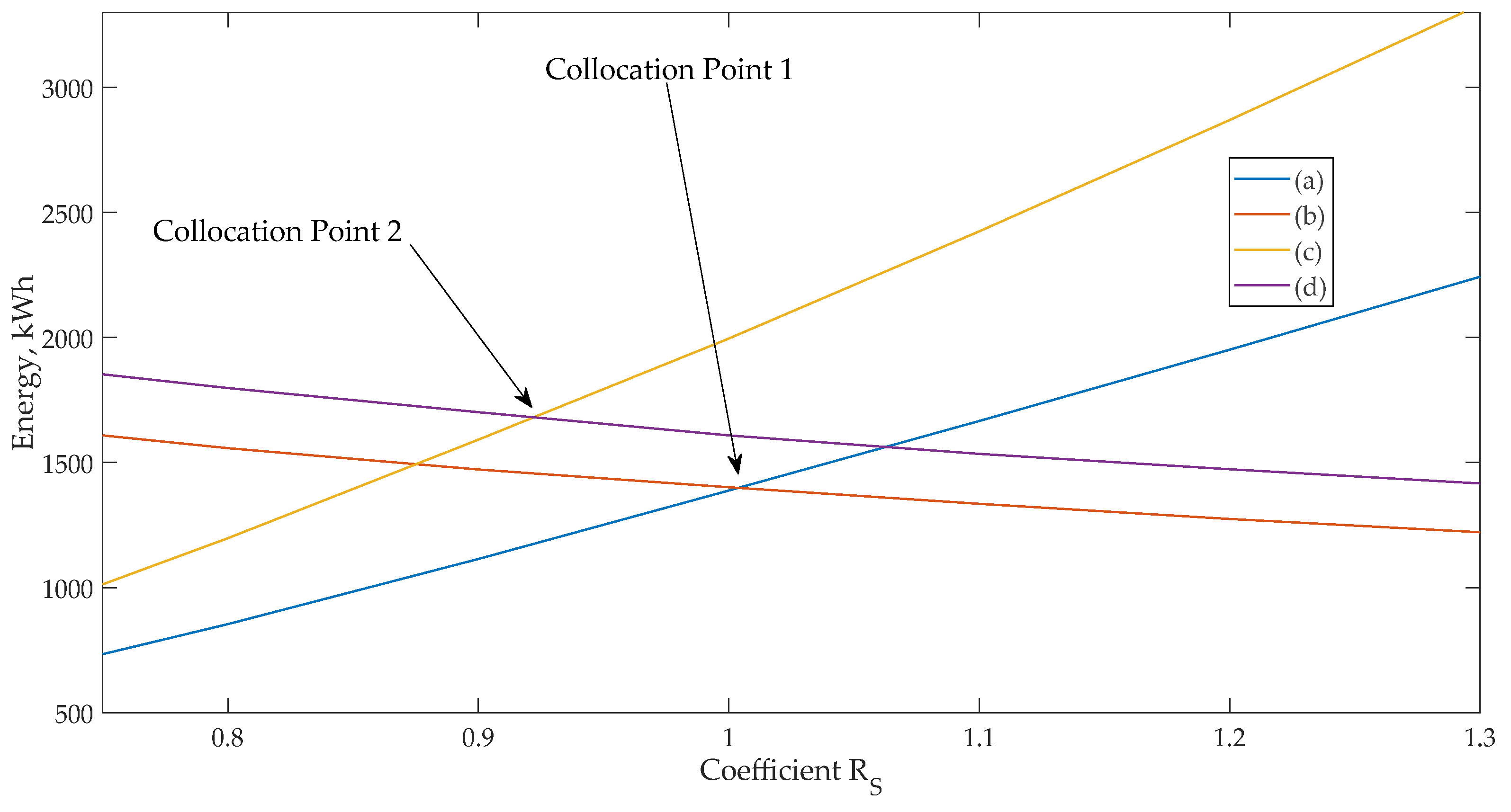
Figure 5 is depicted in the following way. On the horizontal x-axis, the values of amplification coefficient R_S are presented. On the y-axis, we see the energy amounts purchased from the utility grid and exported there. In Figure 5, the line (a) depicts energy flow to the utility grid, without expected production; line (b)—energy flow from the utility grid, without expected production; (c)—energy flow to the utility grid, with considering expected production on 1 h ahead; line (d)—energy flow from the utility grid, with considering expected production of 1 h ahead. Collocation points 1 and 2 correspond to situations where expected production is not considered and where the expected production is considered.

Collocation points 1 and 2 show the coincidence of energy flows between nanogrid and utility grid. Point 1, crossing point of lines (a) and (b), we get without using expected production comparison and collocation point 2 is the crossing point of energy flows (c) and (d), between nanogrid and utility grid with expected production. Figure 5 shows two scenarios: energy flows with the shift of one hour ahead of the expected production and without taking the expected production into account. At collocation point 2 where the expected production is considered for one hour ahead, the value of the amplification coefficient is R_S = 0.93.

Let us analyse the energy flows at R_S = 1. At collocation point 1, W_to = W_from =1393 kWh, i.e., the power flow that goes into the grid and the flow from the grid are equal. It is to be expected as the data are normalised accordingly. By applying the expected production forecast, i.e., R_S = 1, the energy that is import/export into the grid is W_to = 1996 kWh and the energy coming from the grid W_from = 1608 kWh. When using the expected production, the exchange of energy with the grid becomes asymmetric and more intense if compared with the amplification coefficient.

It can be concluded that the optimal WH and SB energy levels are both around 6 kWh at this nanogrid configuration. If a forecast of 1 h ahead, the result is already sufficient for the cover factor’s more significant value. For higher forecast values, the effect is marginal. Suppose the expected production is used 1 h ahead. In that case, the energy stream equality between the utility grid and from the utility grid energy flows at R_S = 0.93 at W_to = W_from = 1393 kWh will already be achieved. Thus, in the case of further increases in R_S, both the W_to and W_from will remain more significant than the expected production. The Y_D will increase from 0.593 to 0.645 in the implementation of the expected output by 0.052.

9. Discussion

Actual data was extracted from a wind generator, installed in a coastal region (N 59.087694, E 23.591719) of Estonia. In the study, the same time series of the wind generator production was used to specify both the energy output in the current time interval and the determined production capacity for 1−5 h ahead as expected output. This approach was chosen because it was necessary to study the possibility of increasing the cover factor Y_D through energy flow management and using the expected wind production in general. The shift of collocation point 2 in Figure 5 towards smaller values of amplification coefficient R_S appears. In the case of expected energy deficit in WG production in the nearest future, the SB in the nanogrid is preferably charged. It is realised by an automatic change in the simulation algorithm under these conditions. Thus, the SB is preferably kept full, and the amount of energy given to the utility grid is reduced. If in the source [42], the cover factor is expressed as a cover factor integral, its physical content is straightforward, defined through Equation (1). Demand cover factor WG describes the energy directly consumed by NS and WH, specifically the power consumed directly from WG in the nanogrid. If WG’s production in a given 5 min period coincides with NS consumption during that period, all or part of the energy produced during that period is consumed in the NS. If there is more energy left, it is going to move on to the WH. Even if there is more power in the WH, it will move on to the battery and, when it is filled, the excess energy will move to UG. Energy entering UG is no longer considered to be under self-consumption. Both consumers NS and WH must have 100% security of supply. If WG does not have enough energy on this 5 min drive for NS, it will be taken from the battery and, even in the event of energy shortages there, the missing part of the UG will be taken, which will not go under self-consumption. Under certain conditions (described in Algorithm 1), in case of lack of energy for B, i.e., hot water production, the missing part of the battery is taken into the WH and insufficient power from the UG there. This energy does not go into self-consumption accounting. It is novel in this solution, which achieves an additional increase in the cover factor.

It should be noted that the changes resulting from the methodology of this regular production monitoring, in practical terms, do not depend on the length of the forecasting time interval. Despite the number of hours projected, there are still reasonable periods in which the projected capacity is less than the present. In real-life conditions, the wind generator’s expected output is calculated based on weather information and characteristics of the wind generator. Naturally, there will be uncertainty in this expectation and this must be taken into account in the energy flow distribution algorithm in future research. Wind as a weather phenomenon is highly stochastic, not only throughout the day but also within long periods of calm and storm. Therefore, it is impossible to compile an annual wind speed model that works in every situation; instead, the storage devices must be controlled according to the near-future conditions. SB and WH capacity selection are relatively subjective, as there are no solid qualitative or quantitative criteria for their choice.

The calculations for a given nanogrid can estimate the impact of the expected production on the value of cover factor and quantities of energy exchanges between the utility grid. In subsequent studies, actual forecast data will examine cover factor behaviour, consider all equipment’s technical characteristics included in the simulation, and introduce the economic analysis.

10. Conclusions

This paper presented a simulation model of energy flows between production and consumption equipment inside a household with a wind generator as its independent electricity source. The paper’s general aim was to develop a self-consumption model using expected production to support the weather forecast. For the efficiency assessment, the cover factor (Equation (1)), also known as the demand cover factor, was used.

The simulation was performed based on data from the average single-family residential house. The data covers the production of wind generator, non-shiftable load, and hot water consumption. A significant result was the demonstration that considering deterministic expected wind generator production makes it possible to increase the cover factor. This motivates further studies of the stochastic prediction of production based on actual weather data.

The outputs of simulations are graphs that explain the influence on the cover factor of some important wind generator parameters, which are the water tank and battery. Modifications are seen in transferring surplus of the wind generator production energy to the utility grid and buying additional energy from the utility grid to fulfil the gap in non-shiftable consumption and water heating.

The results can be used primarily in the design of private prosumer solutions. The method employed can also be applied to other energy systems such as storehouses and industrial objects. The main conclusions are summarised as follows:

• Cover factor Y_D, which was calculated for nanogrid where storage equipment, battery and WH have an energy storage capacity of 6 kWh, is a fairly appropriate indicator for assessment of self-consumption.
• The result, i.e., increasing cover factor Y_D is achievable when the shift of 1 h is considered along with the more significant expected production. Increasing cover factor Y_D is the primary goal of the energy distribution problem.
• Without using expected production period properties Y_D = 0.593 and with deterministic forecast Y_D = 0.645. The cover factor increases by 0.052 or 8.8%.
• Although Y_D increased using the expected production approach, this led to an asymmetric increase in the energy exchange between the nanogrid and the utility grid. The annual amount of energy provided to the utility grid increased concurrently.
• The increase in wind generator energy production for the same consumption level compared to consumption further amplified the YD’s rise for the expected production period.
• It is essential to explore ways to increase the self-consumption of nanogrid users to reduce maintenance costs and the cost of strengthening the utility grid. Increasing local consumption of renewable energy production will reduce grid energy losses and greenhouse gas emissions.