Small-Signal Stability of Multi-Converter Infeed Power Grids with Symmetry

Abstract

Traditional power systems have been gradually shifting to power-electronic-based ones, with more power electronic devices (including converters) incorporated recently. Faced with much more complicated dynamics, it is a great challenge to uncover its physical mechanisms for system stability and/or instability (oscillation). In this paper, we first establish a nonlinear model of a multi-converter power system within the DC-link voltage timescale, from the first principle. Then, we obtain a linearized model with the associated characteristic matrix, whose eigenvalues determine the system stability, and finally get independent subsystems by using symmetry approximation conditions under the assumptions that all converters’ parameters and their susceptance to the infinite bus ($B_g$) are identical. Based on these mathematical analyses, we find that the whole system can be decomposed into several equivalent single-converter systems and its small-signal stability is solely determined by a simple converter system connected to an infinite bus under the same susceptance $B_g$. These results of large-scale multi-converter analysis help to understand the power-electronic-based power system dynamics, such as renewable energy integration. As well, they are expected to stimulate broad interests among researchers in the fields of network dynamics theory and applications.

1. Introduction

The power system is generally believed to be one of the most complicated systems made by human beings, featured with some essential characteristics of complex systems, such as nonlinearity, large spatial scale, multiple timescale, interwinding between coupled elements, etc. [1,2,3]. In a traditional power system dominated by synchronous generators (SGs), the system of electromechanical dynamics is basically controlled by the rotor motion of SG under imbalance torque (or power) [4,5,6]. Its physical picture is clearly understood. Recently the traditional synchronous-generator-dominant power system has been gradually becoming a power-electronic-based one. In particular, with increasing penetration of renewable energy, a large number of devices, such as wind turbines and photovoltaic cells, have been connected to the power grid via power electronic converters, such as voltage source converter (VSC) as a major type of converter [7,8,9,10,11,12,13]. Different from the SG, the converter exhibits a greater complication, due to its diversified structures of the controller. Entangled interaction of controllers within and between converters also makes the system analysis more difficult [14]. Recently, a variety of wide-frequency-band oscillations of power-electronic-based power system have occurred frequently worldwide [2]. A relevant stability analysis has become a hot topic in the fields of both power electronics and power system [1,2,3,14,15,16,17]. Hence it is important and urgent to study the dynamics in a multi-converter system and uncover its stability mechanism.

Although the power-electronic-based power system is intrinsically nonlinear, for simplicity, the classical linear system theory has been extensively applied in the framework of small-signal stability under the condition that the operating point is subjected to a sufficiently small disturbance [4,5,6]. So far, three major methods have been developed, including the modal analysis method in the time domain, and complex torque and impedance methods in the frequency domain [18]. We will apply the modal analysis method as it is common and reliable. In addition, the multi-timescale decomposition technique has also been widely used in reduced-oder modeling and analysis of power-electronic-based power systems. There are several studies concentrating only on one single timescale. For instance, the slow-scale dynamics of VSC was studied within the DC-link voltage timescale by ignoring all fast-scale current controllers [19]. In contrast, it was reported that the fast oscillations can be put into the category of current-timescale by setting all slow-scale controller outputs as constants [20]. We will use the same strategy in our modeling.

On the other hand, the power system stability, as an important problem in realistic complex systems, has also attracted wide interests in physics in the past decade [21,22,23,24,25,26,27,28,29,30,31,32,33,34]. Most studies concentrated on cascade failure [26,27] and synchronization [28,29,30], based on the well-known second-order Kuromoto oscillators and mainly treating the problem how does the network structure shape power grid function. There are few papers on renewable integrations, except some on intermittent behaviors of renewable energies by studying stochastic differential equations [31]. Basically, their timescale is much slower than what we are interested in here. For recent progress on this direction, see, e.g., the focus issues [32,33,34]. Detailed studies on how renewable integration devices work still lack, to the best knowledge of the authors. We would like to stimulate the broad interests of researchers in physics.

Different from a single-converter system, the topologies of a multi-converter system can be diversified. However, due to the comparatively low energy density transferred by a converter, a symmetrical structure has been commonly observed, such as AC microgrid with distributed power sources [35], radial cluster topology of off-shore wind farms [36], grid-connected photovoltaic systems with a radial configuration [37], and multi-infeed VSC power systems [38], etc. The above systems have two common features. One is that the grid-connected devices have similar control structures and parameters, and the other is that the network topology has a certain symmetry. Taking the offshore wind farm as an example, the common topologies are as shown in Figure 1 [39]. Those features bring great convenience to the stability analysis of the multi-converter system. The main conclusions of our work will be based on such property of symmetry.

Based on the above literature review, we find that a generic model of a multi-converter infeed system hasn’t been built yet and the stability mechanism research is still urgently needed. In this paper, relying on the above three major techniques: linearization, multi-timescale decomposition and symmetry analysis, we will establish a nonlinear model of a multi-converter power system within the DC-link voltage timescale from the first principle. Then we will derive a linearized model and conduct linear stability analysis. Finally, by using the mentioned symmetry conditions, we will decompose the multi-converter system into several single-converter subsystems and identify the dominant one for the system’s small-signal stability. We hope those step-by-step modeling and mathematical analysis help to uncover the internal mechanism of the stability of multi-converter infeed system and inspiring for future studies of complicated realistic systems.

The remainder of this paper will be arranged as follows. In Section 2, we establish a nonlinear model of multi-converter infeed power system within the DC-link voltage timescale. In Section 3, the nonlinear model is linearized around the system operation conditions. In Section 4, to obtain the eigenvalues of the characteristic matrix, we make some symmetry assumptions and decouple the whole system into several subsystems. Further analysis finds that only one single-VSC system is dominant in system stability. Section 5 is devoted to simulation results of root loci and time series. Finally, conclusions and discussions are given.In addition, more details about the converter parameters, approximate eigenvalues and the simulation data are represented in the Appendix A, Appendix B and Appendix C.

2. Nonlinear Modeling for Multi-Converter Infeed System

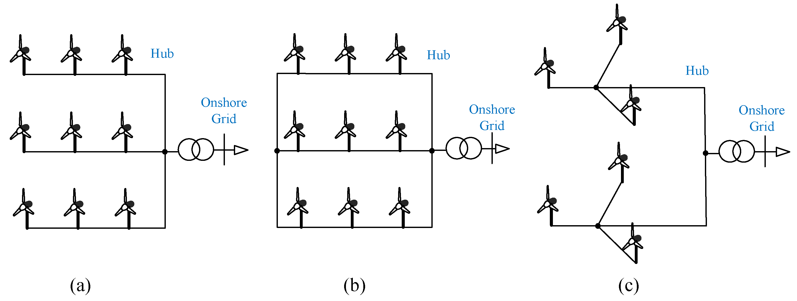
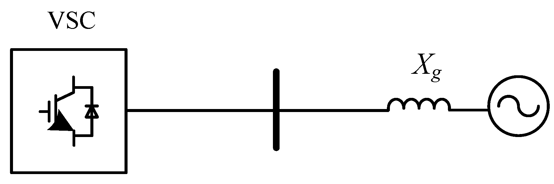
2.1. System Overview

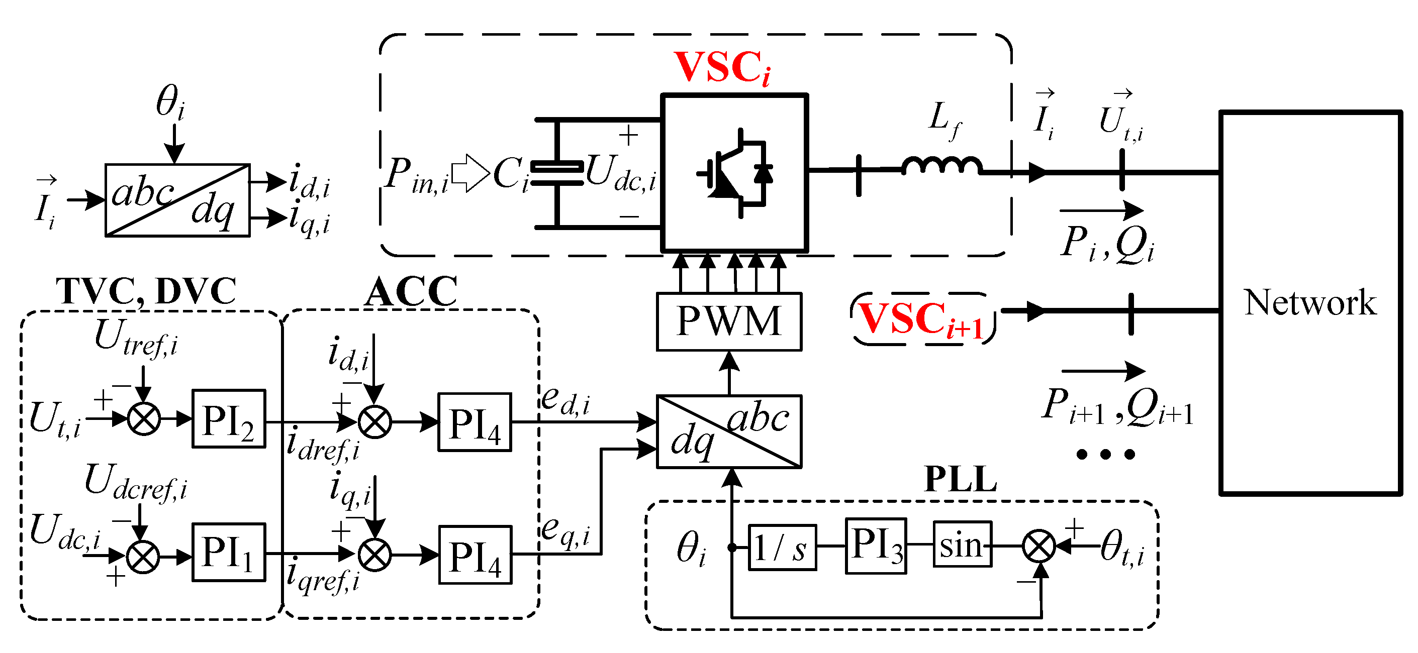
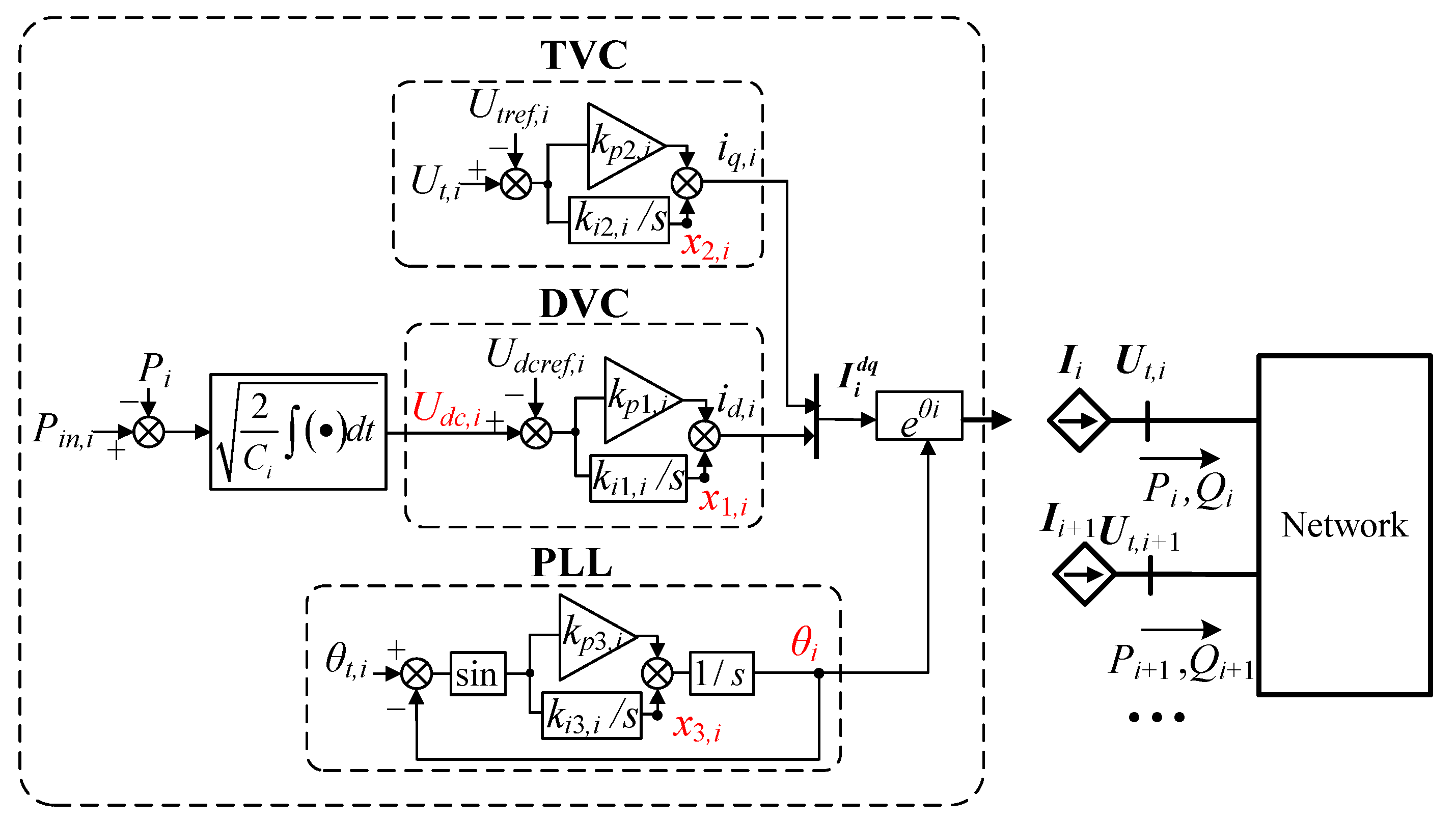
Figure 2a shows the representative and simplified topological structure for a multi-VSC infeed power system within the DC-link voltage control timescale, with each VSC connected to an infinitely strong bus $U_{t,n+1}$ by an inductance. As only slow-scale dynamics are considered, all voltage and current can be expressed as phasors. The system has $n+1$ buses, including n VSC buses and one infinite bus. The infinite bus is numbered as $n+1$ and adopted as the reference bus. Both the voltage amplitude $U_{t,n+1}$ (simplified as $U_g$) and the phase ${\theta }_{t,n+1}$ of the infinite bus are fixed (${\theta }_{t,n+1}=0$).

For the i-th $\left(i=1,2,\cdots ,n\right)$ VSC bus, the voltage amplitude and phase are denoted by $U_{t,i}$ and ${\theta }_{t,i}$, respectively. In our model, for the reactance, $X={\omega }_{0}L$, where ${\omega }_0$ is the fundamental frequency and ${\omega }_0=100\pi$, as $f_0=50$ Hz. As shown in Figure 2a,b, $X_{gi}$ denotes the reactance between the i-th VSC and the infinite bus, termed as the converter-grid reactance, $X_{gi}=X_{ig}$. In contrast, $X_{ij}$ represents the reactance between the i-th and the j-th VSCs, referred to as inter-converter reactance, $X_{ij}=X_{ji}$.

2.2. VSC Modeling

Figure 3 exhibits the detailed control diagram of a multi-VSC power system by utilizing a typical vector control scheme [40,41,42]. The control loops include the terminal voltage control loop (TVC) and DC voltage control loop (DVC) for the outer slow-scale control, and the AC current control loop (ACC) for the inner fast-scale control. In addition, the phase-locked control loop (PLL) for system synchronization belongs to the slow timescale. Different from the $xy$ synchronous reference coordinate rotating at a fixed synchronous speed ${\omega }_0$, the cascaded control loops including the TVC, DVC and ACC should operate on the $dq$ coordinate based on the information of the phase-locked angle ${\theta }_i$ from the PLL. The coordinates and angle relations are illustrated in Figure 4a. The negative feedback controls of the TVC and DVC aim to maintain the terminal voltage and the DC voltage at normal values, respectively. The proportional-integral (PI) linear controllers are adopted in DVC, TVC, and PLL. After the cascade control, the output of the ACC should be transferred back from the $dq$ coordinate to the $xy$ one, serving as gating voltage for six insulated gate bipolar transistors (IGBTs). The waveform change is possible by using the well-known pulse-width modulation (PWM) technique; for more details, see, e.g., [40,41,42].

Clearly the PLL, as a watchdog, plays an important role in the whole control. It provides the phase-locked angle ${\theta }_i$, keeps the converter synchronized with the external grid, and makes the cascade vector controls possible. Figure 4a schematically shows the dynamical relation in the $xy$ synchronous reference coordinate and the $dq$ coordinate, where the phase-locked angle of the PLL, ${\theta }_i$, determines its d-axis orient. In addition, ${\theta }_{t,i}$ denotes the terminal voltage angle, and $u_{td,i}$ and $u_{tq,i}$ are the d- and q-axis components of the terminal voltage, respectively. Finally, to make a comparison, we present some coordinates and angle relations in Figure 4b, but for the synchronous generator instead [4,5,6]. Similarly, the $xy$ frame rotates at a fixed speed ${\omega }_0$ and the $dq$ frame for the rotor position rotates at the rotor speed ${\omega }_i$, which is also time-varying. Generally, ${\delta }_i$ is termed as power angle and ${\theta }_{t,i}$ is the terminal voltage angle. The dynamics of ${\delta }_i$ in SG plays a key role in the system dynamical behavior and is similar to the phase-locked angle ${\theta }_i$ in PLL.

According to the control design criterion, the dynamics of VSC can be roughly divided into the DC-link voltage and current control timescales [7]. For simplicity, in this paper we will only study the DC-link voltage timescale dynamics, by keeping all the outer loops (including the TVC, DVC, and PLL) and neglecting the inner ACC. Hence the current values, $i_{d,i}$ and $i_{q,i}$, should simultaneously follow the current reference values, $i_{dref,i}$ and $i_{qref,i}$. The simplified control diagram is shown in Figure 5. In addition, we can keep the active power input $P_{in,i}$ from the DC-link capacitor in Figure 3 as a constant. As a result, each VSC can be regarded as equivalent to a controlled current source [15], as schematically shown in the right of Figure 5. For the symbols in Figure 5, ($k_{p1,i}$, $k_{i1,i}$), ($k_{p2,i}$, $k_{i2,i}$), and ($k_{p3,i}$, $k_{i3,i}$) represent the PI control parameters of the DVC, TVC, and PLL, respectively. $C_i$ stands for the DC capacitor. $U_{t,i}$ and $U_{tref,i}$ are the terminal voltage and the terminal reference voltage, respectively. $P_{in,i}$ denotes the active power input from the DC side and $P_i$ denotes the active power output via the VSC. ${\theta }_i$ represents the PLL angle, while ${\theta }_{t,i}$ is the terminal voltage angle.

A fifth-order dynamic model of a single VSC has been developed by us recently [9], which will be developed for a detailed modeling of a multi-VSC system. Below we will start from each controller dynamics, network description and establish a whole system model gradually.

For the PI controller in the DVC, the output of the integrator of ${\mathrm{PI}}_1$ is denoted as $x_{1,i}$. Let $x_{1,i}$ be a state variable. Then the DVC can be represented by

$$\stackrel{•}{x_{1,i}}=k_{i1,i}\left(U_{dc,i}-U_{dcref,i}\right),$$

(1)

where the dot represents the time derivative, along with an algebraic equation,

$$i_{d,i}=k_{p1,i}\left(U_{dc,i}-U_{dcref,i}\right)+x_{1,i}.$$

(2)

For the dynamics of the TVC, similarly let $x_{2,i}$ be the output of the integrator of ${\mathrm{PI}}_2$, as a state variable. The TVC dynamics can be described by

$$\stackrel{•}{x_{2,i}}=k_{i2,i}\left(U_{t,i}-U_{tref,i}\right),$$

(3)

and

$$i_{q,i}=k_{p2,i}\left(U_{t,i}-U_{tref,i}\right)+x_{2,i},$$

(4)

where $U_{t,i}$ is the amplitude of the terminal voltage from the network,

$$U_{t,i}=\sqrt{{u_{td,i}}^2+{u_{tq,i}}^2}.$$

(5)

The PLL is composed of not only the ${\mathrm{PI}}_3$ controller, but also another integrator $1/s$, as shown in Figure 5. The output of ${\mathrm{PI}}_3$ is the speed of the $dq$ coordinate, ${\omega }_{pll,i}$, and it is integrated to obtain the phase of the PLL coordinate, ${\theta }_i$. Again we separate the ${\mathrm{PI}}_3$ into one integrator part and the other proportional part, and denote its integrator output as $x_{3,i}$. We choose $x_{3,i}$ and ${\theta }_i$ as state variables and yield the dynamical second-order differential equation of the PLL,

$$\left\{\begin{array}{c}\stackrel{•}{{\theta }_i}=k_{p3,i}sin\left({\theta }_{t,i}-{\theta }_i\right)+x_{3,i}={\omega }_{pll,i},\hfill \\ \stackrel{•}{x_{3,i}}=k_{i3,i}sin\left({\theta }_{t,i}-{\theta }_i\right).\hfill \end{array}\right.$$

(6)

From Figure 4a, we get the so-called phase-locked angle error:

$${\theta }_{t,i}-{\theta }_i=arctan\left(\frac{u_{tq,i}}{u_{td,i}}\right).$$

(7)

Note that in the steady-state, ${\theta }_{t,i}={\theta }_i$ and $u_{tq,i}=0$.

Next for the DC capacitor, its dynamics is determined by the imbalance active power between the input and output of the VSC, i.e.,

$$d\left(\frac{1}{2}C{U^2}_{dc,i}\right)/\phantom{d\left(\frac{1}{2}C{U^2}_{dc,i}\right)dt}dt=P_{in,i}-P_i,$$

(8)

or

$$\stackrel{•}{U_{dc,i}}=\frac{1}{C_i{U}_{dc,i}}\left(P_{in,i}-P_i\right),$$

(9)

where $P_{in,i}$ is assumed to be a constant in our model and $P_i$ denotes the output active power, determined by

$$P_i=u_{td,i}{i}_{d,i}+u_{tq,i}{i}_{q,i}.$$

(10)

Finally, we can combine the dynamical Equations (1), (3), (6), and (9), and get the following fifth-order differential equations for each VSC:

$$\left\{\begin{array}{c}\stackrel{•}{x_{1,i}}=k_{i1,i}\left(U_{dc,i}-U_{dcref,i}\right),\hfill \\ \stackrel{•}{x_{2,i}}=k_{i2,i}\left(U_{t,i}-U_{tref,i}\right),\hfill \\ \stackrel{•}{{\theta }_i}=k_{p3,i}sin\left({\theta }_{t,i}-{\theta }_i\right)+x_{3,i},\hfill \\ \stackrel{•}{x_{3,i}}=k_{i3,i}sin\left({\theta }_{t,i}-{\theta }_i\right),\hfill \\ \stackrel{•}{U_{dc,i}}=\left(P_{in,i}-P_i\right)/\left(C_i{U}_{dc,i}\right).\hfill \end{array}\right.$$

(11)

Clearly $x_{1,i}$, $x_{2,i}$, $x_{3,i}$, ${\theta }_i$, and $U_{dc,i}$ are five state variables, marked red in Figure 5, where $x_{1,i}$, $x_{2,i}$, and $x_{3,i}$ are the outputs of the integrators of the corresponding PI controllers. The input variables from the network are $u_{td,i}$ and $u_{tq,i}$. In contrast, as the VSC can be regarded as a controlled current, $i_{d,i}$ in (2) and $i_{q,i}$ in (4) are set as the VSC outputs. In addition, substituting (5), (7), and (10) into (3), (4), (6), and (8), $U_{t,i}$, ${\theta }_{t,i}$, and $P_i$ as intermediate variables can be removed and further represented by $u_{td}$ and $u_{tq}$.

In summary, the dynamic model for each VSC is composed of the state-space Equation (11), along with the input Equations (5), (7), and (10) and the output Equations (2) and (4), showing highly interwoven nonlinear relations between these variables.

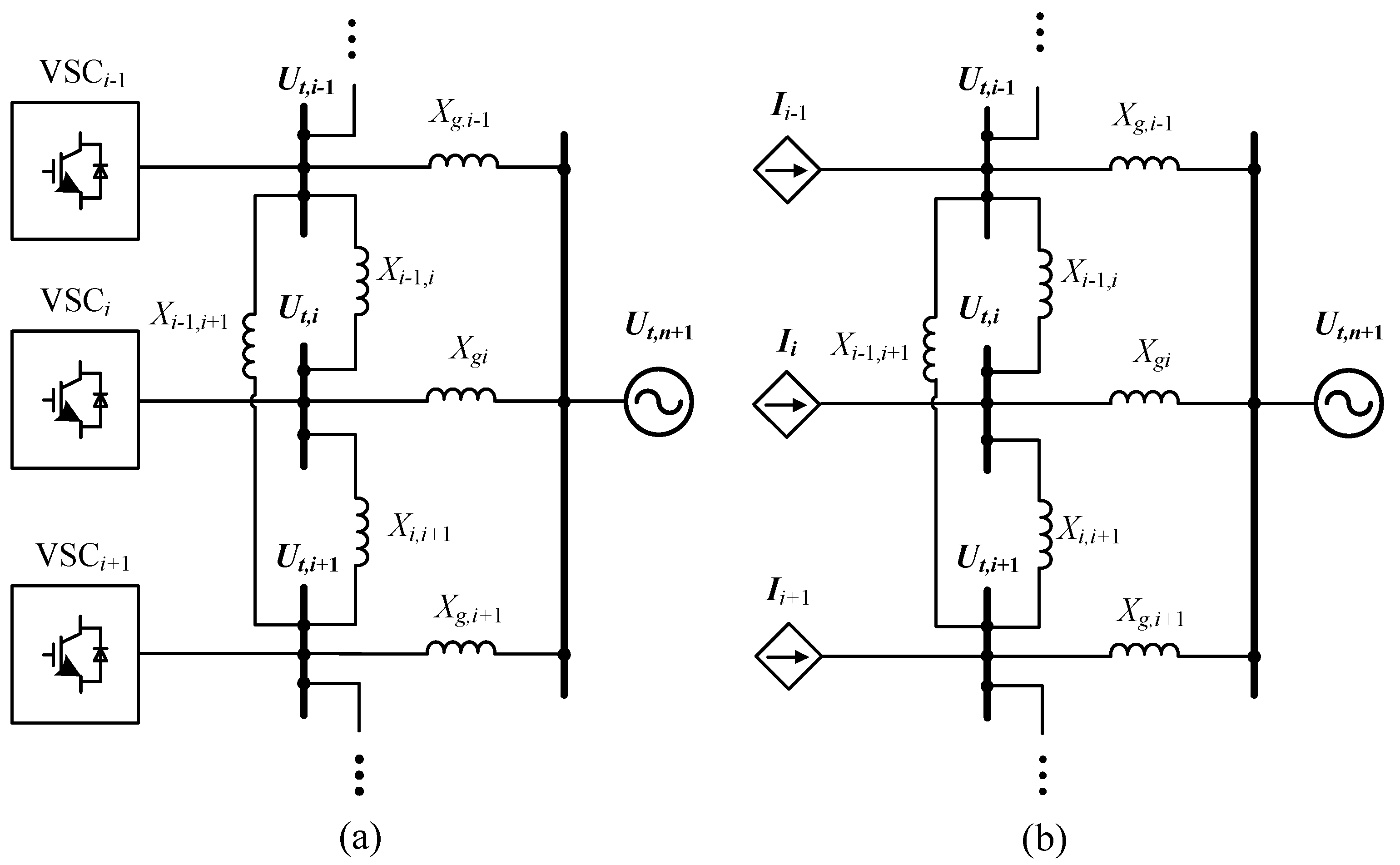
2.3. Network Modeling

For simplicity, we only consider inductance and neglect resistance and conductance. Based on the network topology in Figure 2 and applying the electric circuit theory [43], the mutual-susceptance between the device buses i and j, $B_{ij}$ (or called inter-converter susceptance), and the self-susceptance of the i-th device bus, $B_{ii}$, can be expressed as, respectively,

$$B_{ij}=\frac{1}{X_{ij}}=B_{ji}=\frac{1}{X_{ji}},$$

(12)

and

$$B_{ii}=\sum _{j=1,j\ne i}^n\frac{1}{X_{ij}}+\frac{1}{X_{gi}}=\sum _{j=1,j\ne i}^n{B}_{ij}+B_{gi}.$$

(13)

Similarly, the mutual-susceptance between the i-th VSC bus and the infinite bus, $B_{gi}$ (or called converter-grid susceptance), and the self-susceptance of the infinite bus $B_{gg}$ can be expressed as, respectively,

$$B_{gi}=\frac{1}{X_{gi}}=B_{ig}=\frac{1}{X_{ig}},$$

(14)

and

$$B_{gg}=\sum _{i=1}^n{B}_{gi}.$$

(15)

With the voltage and current phasors, the bus admittance equation of the network [43] is

$$\left[\begin{array}{c}\overrightarrow{I_1}\\ ⋮\\ \overrightarrow{I_n}\\ \overrightarrow{I_{n+1}}\end{array}\right]=\left[\begin{array}{cccc}-j{B}_{11}& \cdots & j{B}_{1n}& j{B}_{g1}\\ ⋮& \ddots & ⋮& ⋮\\ j{B}_{n1}& \cdots & -j{B}_{nn}& j{B}_{gn}\\ j{B}_{g1}& \cdots & j{B}_{gn}& -j{B}_{gg}\end{array}\right]\left[\begin{array}{c}\overrightarrow{U_{t,1}}\\ ⋮\\ \overrightarrow{U_{t,n}}\\ \overrightarrow{U_{t,n+1}}\end{array}\right],$$

(16)

where $\overrightarrow{I_i}=i_{x,i}+j{i}_{y,i}$ and $\overrightarrow{U_{t,i}}=u_{tx,i}+j{u}_{ty,i}$ for $i=1,2,...,n+1$. $j=\sqrt{-1}$. We can further derive the network admittance equation in the $xy$ synchronous coordinate, as shown in (19).

As mentioned before, the i-th VSC accepts voltage as inputs ($u_{td,i}$ and $u_{tq,i}$) from the network, and meanwhile provides current as outputs ($i_{d,i}$ and $i_{q,i}$) to the network. The coordinate transformations of these voltage and current between the $dq$ coordinate and the $xy$ coordinate are needed; based on Figure 4, we get

$$\left[\begin{array}{c}{u}_{td,i}\\ u_{tq,i}\end{array}\right]=\left[\begin{array}{cc}cos{\theta }_i& sin{\theta }_i\\ -sin{\theta }_i& cos{\theta }_i\end{array}\right]\left[\begin{array}{c}{u}_{tx,i}\\ u_{ty,i}\end{array}\right]$$

(17)

$$\left[\begin{array}{c}{i}_{d,i}\\ i_{q,i}\end{array}\right]=\left[\begin{array}{cc}cos{\theta }_i& sin{\theta }_i\\ -sin{\theta }_i& cos{\theta }_i\end{array}\right]\left[\begin{array}{c}{i}_{x,i}\\ i_{y,i}\end{array}\right]$$

(18)

From (16), we obtain

$$\left[\begin{array}{c}{i}_{x,1}\\ i_{y,1}\\ ⋮\\ i_{x,n}\\ i_{y,n}\\ i_{x,n+1}\\ i_{x,n+1}\end{array}\right]=\left[\begin{array}{ccccccc}0& B_{11}& \cdots & 0& -B_{1n}& 0& -B_{g1}\\ -B_{11}& 0& \cdots & B_{1n}& 0& B_{g1}& 0\\ ⋮& ⋮& \ddots & ⋮& ⋮& ⋮& ⋮\\ 0& -B_{n1}& \cdots & 0& B_{nn}& 0& -B_{gn}\\ B_{n1}& 0& \cdots & -B_{nn}& 0& B_{gn}& 0\\ 0& -B_{g1}& \cdots & 0& -B_{gn}& 0& B_{gg}\\ B_{g1}& 0& \cdots & B_{gn}& 0& -B_{gg}& 0\end{array}\right]\left[\begin{array}{c}{u}_{tx,1}\\ u_{ty,1}\\ ⋮\\ u_{tx,n}\\ u_{ty,n}\\ u_{tx,n+1}\\ u_{tx,n+1}\end{array}\right].$$

(19)

Combining the above (17), (18) and (19) yields

$$\left[\begin{array}{c}{i}_{d,1}\\ i_{q,1}\\ ⋮\\ i_{d,n}\\ i_{q,n}\\ i_{d,n+1}\\ i_{q,n+1}\end{array}\right]={\mathit{Y}}_a\left[\begin{array}{c}{u}_{td,1}\\ u_{tq,1}\\ ⋮\\ u_{td,n}\\ u_{tq,n}\\ u_{td,n+1}\\ u_{tq,n+1}\end{array}\right]$$

(20)

where

$${\mathit{Y}}_a=\left[\begin{array}{ccccccc}0& B_{11}& \cdots & B_{1n}sin{\theta }_{1n}& -B_{1n}cos{\theta }_{1n}& B_{g1}sin{\theta }_1& -B_{g1}cos{\theta }_1\\ -B_{11}& 0& \cdots & B_{1n}cos{\theta }_{1n}& B_{1n}sin{\theta }_{1n}& B_{g1}cos{\theta }_1& B_{g1}sin{\theta }_1\\ ⋮& ⋮& \ddots & ⋮& ⋮& ⋮& ⋮\\ B_{n1}sin{\theta }_{n1}& -B_{n1}cos{\theta }_{n1}& \cdots & 0& B_{nn}& B_{gn}sin{\theta }_n& -B_{gn}cos{\theta }_n\\ B_{n1}cos{\theta }_{n1}& B_{n1}sin{\theta }_{n1}& \cdots & -B_{nn}& 0& B_{gn}cos{\theta }_n& B_{gn}sin{\theta }_n\\ -B_{g1}sin{\theta }_1& -B_{g1}cos{\theta }_1& \cdots & -B_{gn}sin{\theta }_n& -B_{gn}cos{\theta }_n& 0& B_{gg}\\ B_{g1}cos{\theta }_1& -B_{g1}sin{\theta }_1& \cdots & B_{gn}cos{\theta }_n& -B_{gn}sin{\theta }_n& -B_{gg}& 0\end{array}\right]$$

(21)

${\theta }_{ij}={\theta }_i-{\theta }_j$ in (21) denotes the phase-locked angle mismatch between i and j. Note that we will always use bold to represent a matrix in the paper.

2.4. Whole System Modeling

Clearly Equations (11) and (20), along with the input Equations (5), (7), and (10) and the output Equations (2) and (4) as the interface between VSCs and network, have constituted a nonlinear model for the whole multi-VSC infeed system within the DVC timescale. In this picture, each node serves as a controlled current source, whereas the network works as a reservoir for the interaction. In addition, we like to emphasize that differing from the usual treatment in power system analysis in textbooks [4], where the whole system is analyzed within the common $xy$ synchronous coordinate, here oppositely we keep each VSC within its own PLL coordinate and deal with the interaction on the network within the $dq$ coordinate of each VSC. Actually, it keeps the converter inner structure and makes system modeling and analysis more convenient.

3. Linear Modeling for Multi-Converter Infeed System

Now we like to step further for a small perturbation analysis, in the fashion of power electrical engineering [4]. Therefore, the above nonlinear equations will be linearized around the operating point (or called fixed point in the nonlinear dynamics field) with the linear system theory employed.

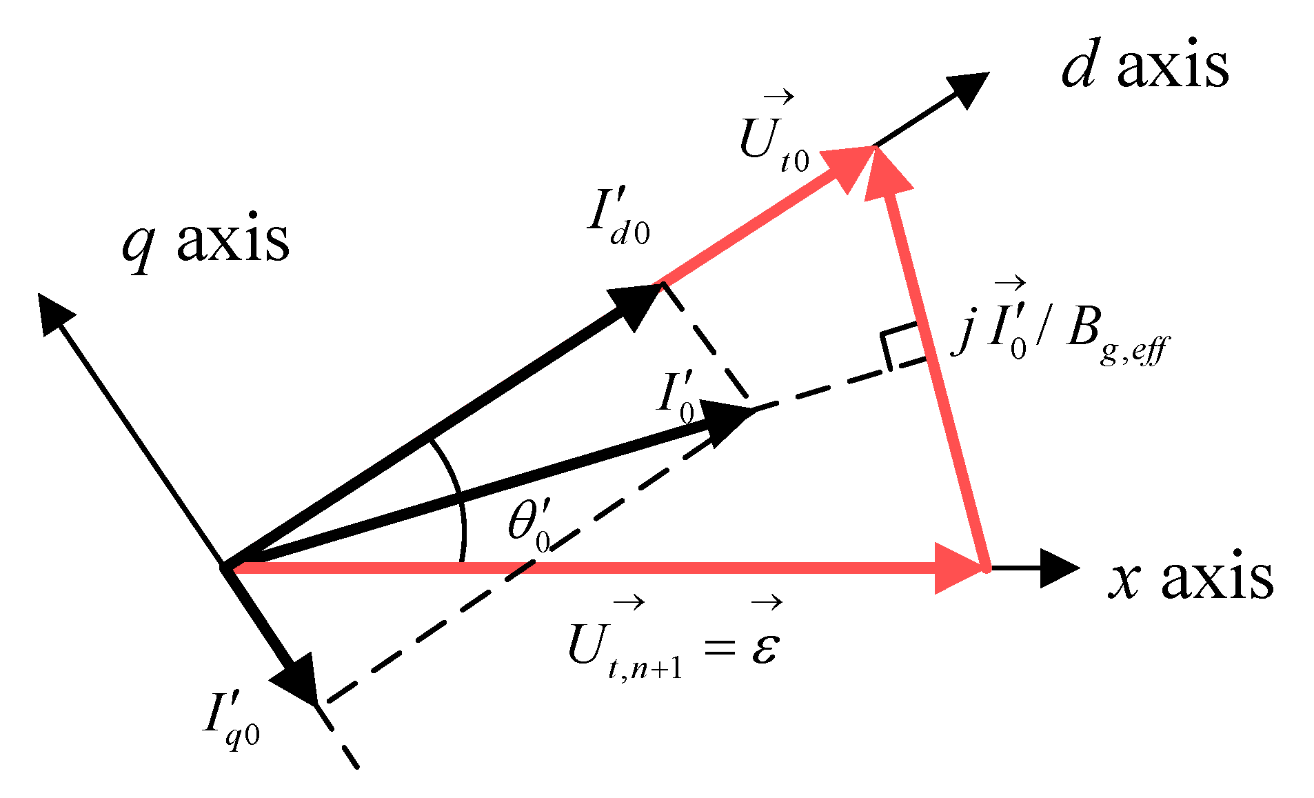
3.1. Operating Point

By setting the right side of (11) equal zero, the operating point can be solved: $U_{t0,i}=U_{tref,i}$, ${\theta }_{i0}={\theta }_{t0,i}$, and thus $u_{d0,i}=U_{t0,i}$ and $u_{q0,i}=0$. $U_{dc0,i}=U_{dcref,i}$, $P_{i0}=P_{in,i}$. We will always use the subscript 0 to represent the operating point under the steady-state. Let $U_{t0,i}=U_{dc0,i}=1$ in the per unit system, to simplify the calculation. In addition, $U_g=1$ for the infinite bus. In this way, the output power $P_{i0}$ and the terminal voltage amplitude $U_{t0,i}$ of each VSC can be obtained. By treating these VSC buses as PV buses, the system steady-state can be analyzed by solving the so-called power flow [4,5,6]. As a result, we obtain the current at the operating point $i_{d0,i}$ and $i_{q0,i}$, and the steady-state phase-lock angle ${\theta }_{i0}$. All parameters are listed in Appendix A.

3.2. VSC Linearization

The state variable of VSC is denoted by

$$\Delta {\mathit{X}}_{\mathit{VSC},\mathit{i}}={\left[\Delta x_{1,i},\Delta x_{2,i},\Delta {\theta }_i,\Delta x_{3,i},\Delta U_{dc,i}\right]}^T$$

(22)

The state-space equations for VSCs can be inferred by linearizing (11). Here we use the prefix $\Delta$ to represent a small-signal variable. The output of VSC (also the network input) is denoted by

$$\Delta \mathit{I}{}_i={\left[\Delta i_{d,i}\Delta i_{q,i}\Delta {\theta }_i\right]}^T.$$

(23)

For convenience of matrix calculation later, here we also add $\Delta {\theta }_i$ in the input variables of VSC,

$$\Delta \mathit{U}{}_i={\left[\Delta u_{d,i}\Delta u_{q,i}\Delta {\theta }_i\right]}^T.$$

(24)

As a result, by linearizing and combining (5), (7), (10), and (11), we get the small-signal state-space equations of VSC in the matrix form

$$\stackrel{•}{\Delta {\mathit{X}}_{\mathit{VSC},\mathit{i}}}=\mathit{F}{}_i\Delta {\mathit{X}}_{\mathit{vsc},\mathit{i}}+\mathit{H}{}_i\Delta \mathit{U}{}_i,$$

(25)

where

$$\mathit{F}{}_i=\left[\begin{array}{ccccc}0& 0& 0& 0& k_{i1,i}\\ 0& 0& 0& 0& 0\\ 0& 0& 0& 1& 0\\ 0& 0& 0& 0& 0\\ -\frac{1}{C_i}& 0& 0& 0& -\frac{k_{p1,i}}{C_i}\end{array}\right],\mathit{H}{}_i=\left[\begin{array}{ccc}0& 0& 0\\ k_{i2,i}& 0& 0\\ 0& k_{p3,i}& 0\\ 0& k_{i3,i}& 0\\ -\frac{i_{d0,i}}{C_i}& -\frac{i_{q0,i}}{C_i}& 0\end{array}\right].$$

(26)

Note that the last column of $\mathit{H}{}_i$ is all zero, indicating that the $\Delta {\theta }_i$ in $\Delta \mathit{U}{}_i$ has no any effect according to (25).

Correspondingly, the VSC output matrix can be obtained by linearizing and combining (2), (4), and (5),

$$\Delta \mathit{I}{}_i=\mathit{J}{}_i\Delta {\mathit{X}}_{\mathit{vsc},\mathit{i}}+\mathit{K}{}_i\Delta {\mathit{U}}_{\mathit{i}},$$

(27)

where

$${\mathit{J}}_i=\left[\begin{array}{ccccc}1& 0& 0& 0& k_{p1,i}\\ 0& 1& 0& 0& 0\\ 0& 0& 1& 0& 0\end{array}\right],{\mathit{K}}_i=\left[\begin{array}{ccc}0& 0& 0\\ k_{p2,i}& 0& 0\\ 0& 0& 0\end{array}\right].$$

(28)

Note also that among the four matrices $\mathit{F}{}_i$, $\mathit{H}{}_i$, $\mathit{J}{}_i$, and $\mathit{K}{}_i$, only $\mathit{H}{}_i$ depends on the steady-state values of $i_{d0,i}$ and $i_{q0,i}$, whereas all other matrices depend on fixed system parameters only.

3.3. Network Linearization

The network Equation (20) should also be linearized. As we know, there are $n+1$ buses with three input or output variables for each bus, as shown in (23) and (24). The dimension of the linear nodal admittance matrix should be $3(n+1)\times 3(n+1)$. However, as the voltage amplitude and phase on the infinite $(n+1)$-th bus are constant ($U_g=1$ and ${\theta }_{t,n+1}=0$), their perturbed variables can be eliminated completely. We obtain the final linear nodal admittance matrix ${\mathit{Y}}_c$ with the dimension of $3n\times 3n$:

$$\left[\begin{array}{c}\Delta \mathit{I}{}_1\\ ⋮\\ \Delta \mathit{I}{}_n\end{array}\right]=\mathit{Y}{}_c\left[\begin{array}{c}\Delta \mathit{U}{}_1\\ ⋮\\ \Delta \mathit{U}{}_n\end{array}\right],$$

(29)

where $\mathit{Y}{}_c$ can be divided into the $n\times n$ partitioned matrix

$$\mathit{Y}{}_c=\left[\begin{array}{cccc}{\mathit{Y}}_{\mathit{c},\mathit{11}}& {\mathit{Y}}_{\mathit{c},\mathit{12}}& \cdots & {\mathit{Y}}_{\mathit{c},\mathit{1}\mathit{n}}\\ {\mathit{Y}}_{\mathit{c},\mathit{21}}& {\mathit{Y}}_{\mathit{c},\mathit{22}}& \cdots & {\mathit{Y}}_{\mathit{c},\mathit{2}\mathit{n}}\\ ⋮& ⋮& \ddots & ⋮\\ {\mathit{Y}}_{\mathit{c},\mathit{n}\mathit{1}}& {\mathit{Y}}_{\mathit{c},\mathit{n}\mathit{2}}& \cdots & {\mathit{Y}}_{\mathit{c},\mathit{nn}}\end{array}\right]$$

(30)

with the diagonal block of ${\mathit{Y}}_{\mathit{c}}$ expressed as

$${\mathit{Y}}_{\mathit{c},\mathit{ii}}={\left[\begin{array}{ccc}0& B_{ii}& B_{gi}cos{\theta }_{i0}+{\displaystyle \sum _{j=1,j\ne i}^n}{B}_{ij}cos{\theta }_{ij0}\\ -B_{ii}& 0& -B_{gi}sin{\theta }_{i0}-{\displaystyle \sum _{j=1,j\ne i}^n}{B}_{ij}sin{\theta }_{ij0}\\ 0& 0& 1\end{array}\right]}_{3\times 3}$$

(31)

and the off-diagonal blocks of ${\mathit{Y}}_c$ ($i\ne j$) expressed as

$${\mathit{Y}}_{\mathit{c},\mathit{ij}}={\left[\begin{array}{ccc}{B}_{ij}sin{\theta }_{ij0}& -B_{ij}cos{\theta }_{ij0}& -B_{ij}cos{\theta }_{ij0}\\ B_{ij}cos{\theta }_{ij0}& B_{ij}sin{\theta }_{ij0}& B_{ij}sin{\theta }_{ij0}\\ 0& 0& 0\end{array}\right]}_{3\times 3}$$

(32)

Here ${\theta }_{ij0}={\theta }_{i0}-{\theta }_{j0}$ denotes the phase-locked angle difference between i and j under the steady-state.

3.4. Characteristic Equation for Linear System Modeling

Finally, by combining (25), (27), and (29), and eliminating $\Delta \mathit{U}{}_i$ and $\Delta \mathit{I}{}_i$, we get the linearized model,

$$\stackrel{•}{\Delta {\mathit{X}}_{\mathit{VSC},\mathit{i}}}=\mathit{A}\Delta {\mathit{X}}_{\mathit{VSC},\mathit{i}},$$

(33)

where the small-signal stability should be determined by $\mathit{A}$; $\mathit{A}$ is the characteristic matrix with the dimension of $5n\times 5n$,

$$\mathit{A}=\mathit{F}+\mathit{H}{({\mathit{Y}}_c-\mathit{K})}^{-1}\mathit{J}$$

(34)

with $\mathit{F}$, $\mathit{H}$, $\mathit{J}$, and $\mathit{K}$ being all n-block diagonal partitioned matrices,

$$\begin{array}{c}\mathit{F}=diag(\mathit{F}{}_1,\dots ,\mathit{F}{}_n),\hfill \\ \mathit{H}=diag(\mathit{H}{}_1,\dots ,\mathit{H}{}_n),\hfill \\ \mathit{J}=diag(\mathit{J}{}_1,\dots ,\mathit{J}{}_n),\hfill \\ \mathit{K}=diag(\mathit{K}{}_1,\dots ,\mathit{K}{}_n).\hfill \end{array}$$

(35)

Now we have established the complete state-space model of the n-VSC system after knowing all system parameters and the steady-state operating points through power flow calculation. We get the unified mathematical form of the characteristic matrix which can be directly extended into the system of any number of VSCs. If all eigenvalues of $\mathit{A}$ are located in the left-half-plane, the system would be locally stable. In this way, the eigenvalue calculation of a huge matrix $\mathit{A}$ should be conducted. Below, however, we like to step ahead for a possible order reduction and search for a physical result.

4. Small-Signal Stability Analysis for Multi-Converter Infeed System with Symmetry

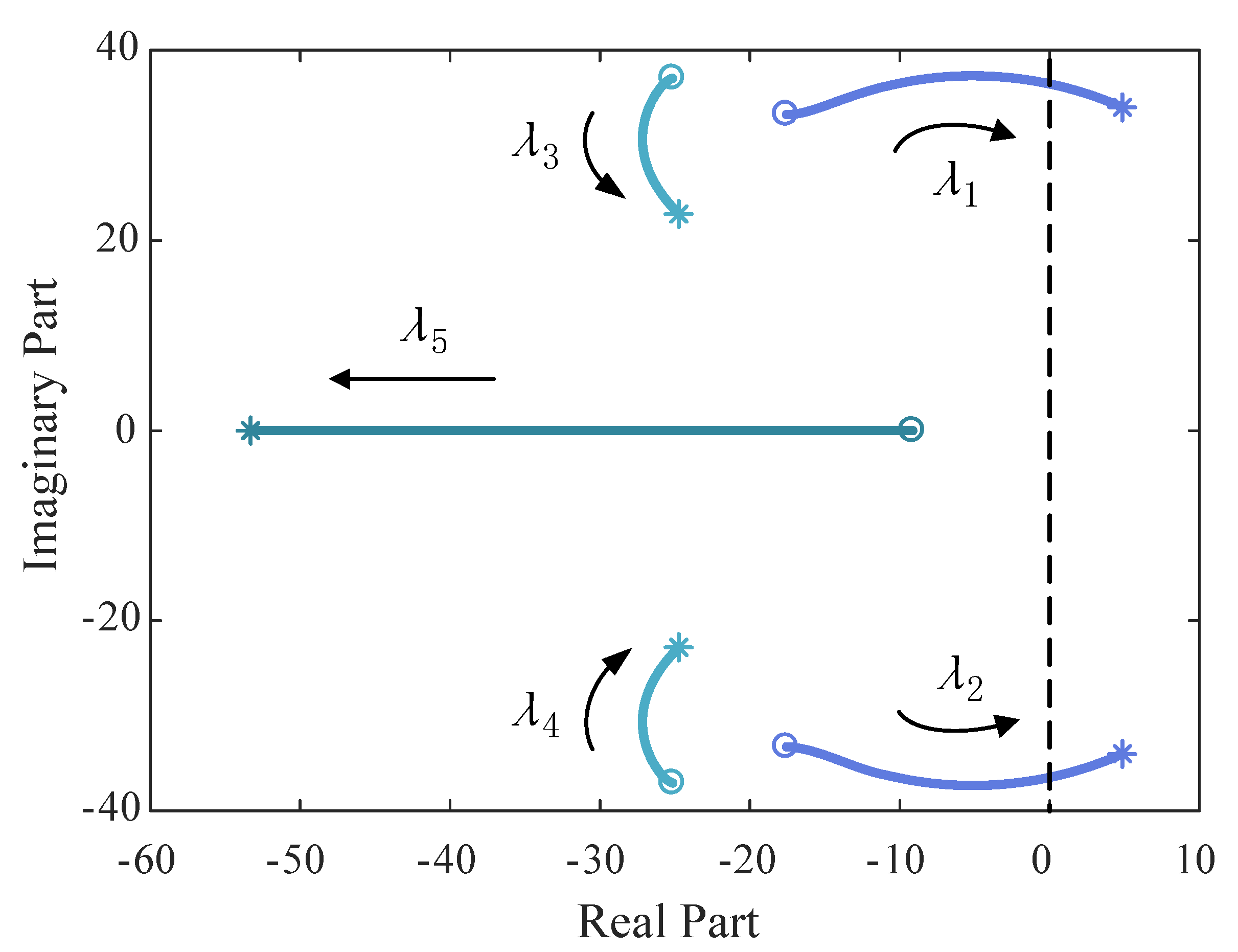
4.1. Small-Signal Stability Analysis for a Single VSC System

First, we start from the simplest case of a single VSC infeed system in Figure 6, where the VSC-grid reactance $X_g$ represents the reactance between the VSC and the infinite grid. Under this situation, the characteristic matrix can be easily obtained from (34),

$${\mathit{A}}_{\mathit{single}}=\mathit{F}{}_s+{\mathit{H}}_s{({\mathit{Y}}_{\mathit{c},\mathit{single}}-\mathit{K}{}_s)}^{-1}\mathit{J}{}_s,$$

(36)

where $\mathit{F}{}_s$ ($\mathit{F}{}_s=\mathit{F}{}_1$), $\mathit{H}{}_s$ ($\mathit{H}{}_s=\mathit{H}{}_1$), $\mathit{J}{}_s$ ($\mathit{J}{}_s=\mathit{J}{}_1$), and $\mathit{K}{}_s$ ($\mathit{K}{}_s=\mathit{K}{}_1$) correspond to the only one block matrix determined by the single VSC in (26) and (28), with the corresponding network matrix derived from ${\mathit{Y}}_{\mathit{c},\mathit{ii}}$ in (31),

$${\mathit{Y}}_{\mathit{c},\mathit{single}}=\left[\begin{array}{ccc}0& B_g& B_{g}cos{\theta }_0\\ -B_g& 0& -B_{g}sin{\theta }_0\\ 0& 0& 1\end{array}\right].$$

(37)

Here, the VSC-grid susceptance $B_g=1/\phantom{1X_g}{X}_g$ and ${\theta }_0$ denotes the steady-state value of the phase-locked angle of the single VSC.

For such a small system, the five eigenvalues of ${\mathit{A}}_{\mathit{single}}$ in (36) can be easily calculated. We will see that this simple-converter system plays a crucial role in our multi-converter system stability analysis.

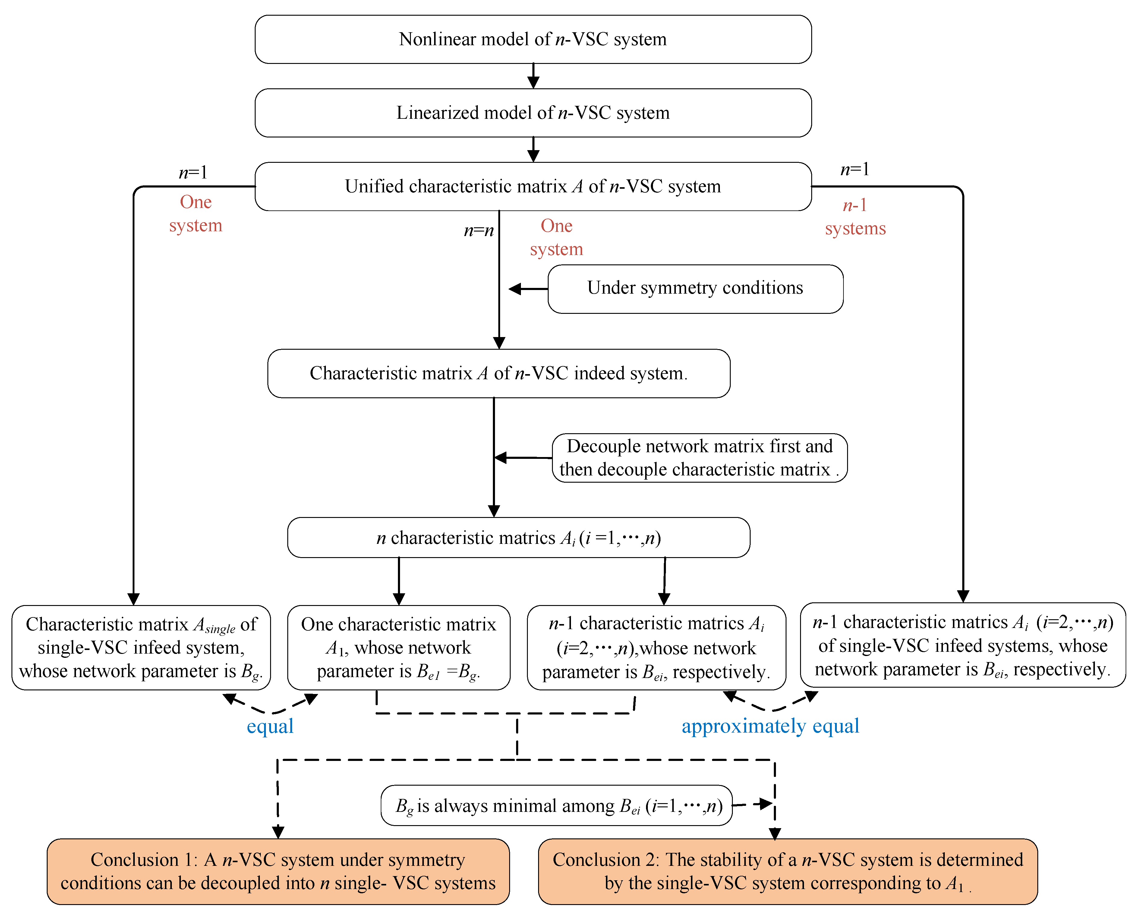
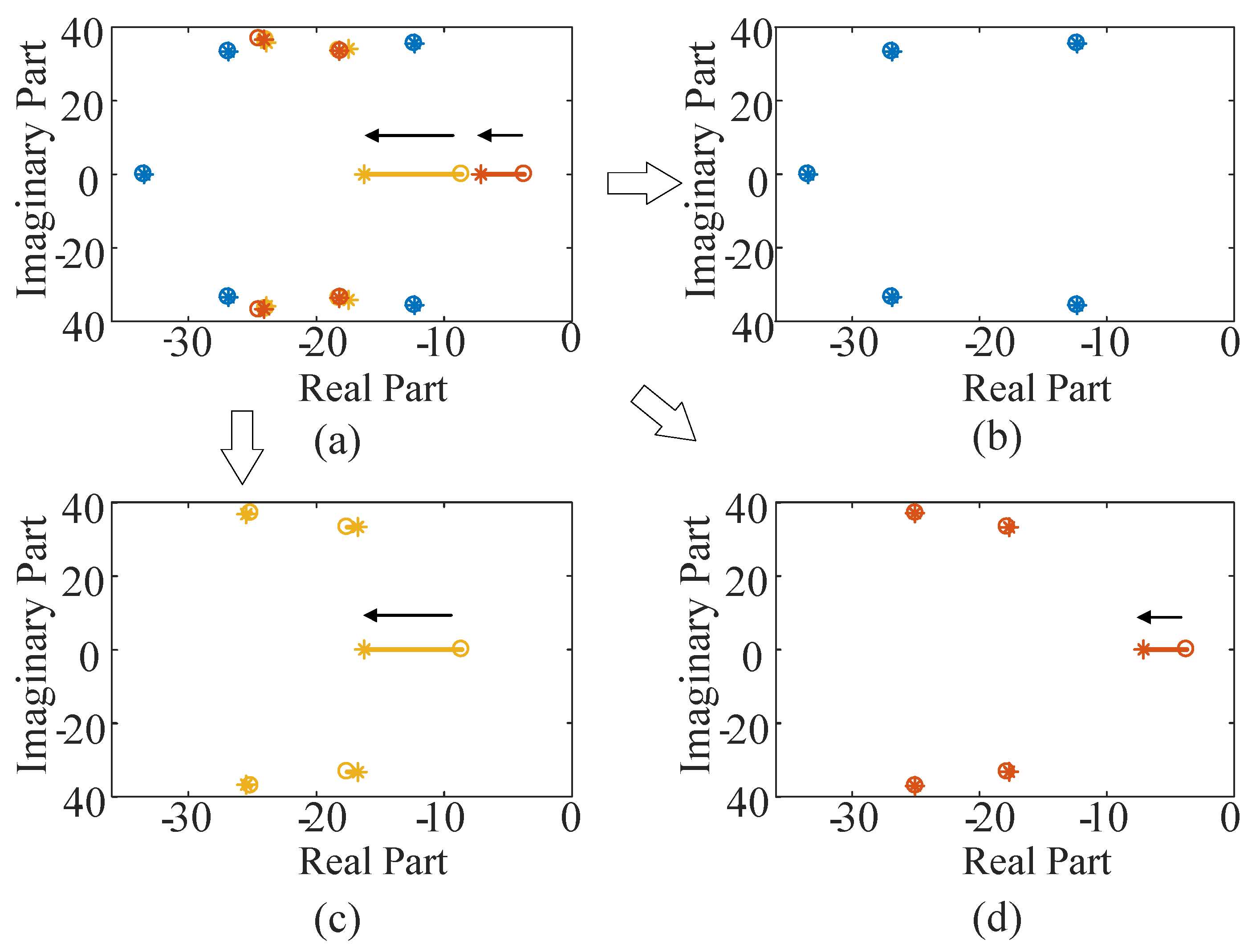
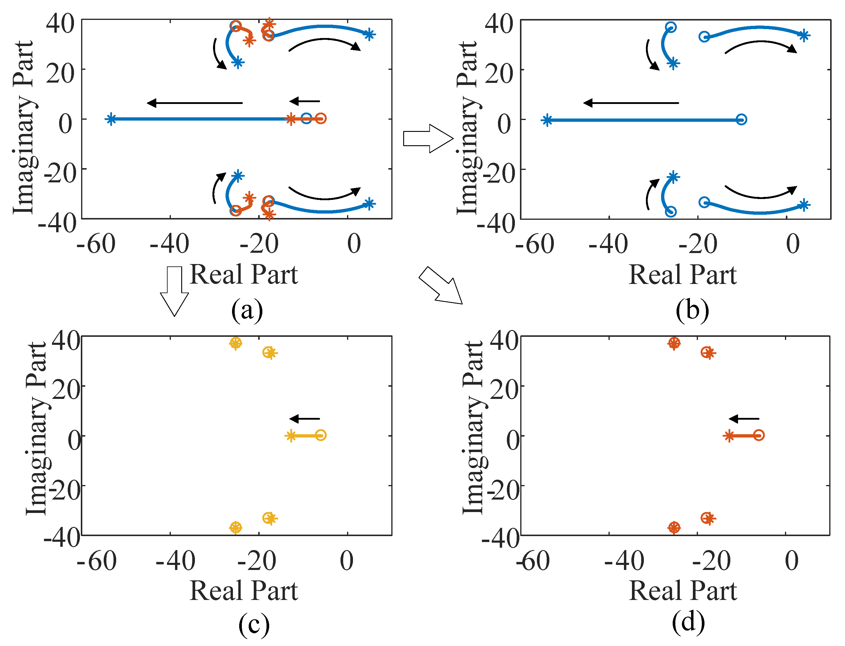
4.2. Decoupling of Multi-VSC Infeed System with Symmetry

Now to analyze the multi-VSC infeed system, we consider some symmetry assumptions. As the first assumption, all VSCs should have the same control loops, control parameters, and DC capacity. Hence $\mathit{F}{}_i$, $\mathit{H}{}_i$, $\mathit{J}{}_i$, and $\mathit{K}{}_i$ are all identical and can be simplified as $\mathit{F}{}_s$, $\mathit{H}{}_s$, $\mathit{J}{}_s$, and $\mathit{K}{}_s$, respectively. Therefore, we get

$$\begin{array}{c}\mathit{F}=diag(\mathit{F}{}_s,\dots ,\mathit{F}{}_s),\hfill \\ \mathit{H}=diag(\mathit{H}{}_s,\dots ,\mathit{H}{}_s),\hfill \\ \mathit{J}=diag(\mathit{J}{}_s,\dots ,\mathit{J}{}_s),\hfill \\ \mathit{K}=diag(\mathit{K}{}_s,\dots ,\mathit{K}{}_s),\hfill \end{array}$$

(38)

corresponding to the original (35).

In addition, ${\mathit{Y}}_c$ in (34) should also be decoupled and then the characteristic matrix $\mathit{A}$ is solvable. Observing that both ${\mathit{Y}}_{\mathit{c},\mathit{ii}}$ in (31) and ${\mathit{Y}}_{\mathit{c},\mathit{ij}}$ (32) highly depend on the steady-state phase-locked angle difference ${\theta }_{ij0}$ (${\theta }_{ij0}={\theta }_{i0}-{\theta }_{j0}$), we can make the second assumption that the VSC-grid susceptance $B_{ig}$ should be identical. It is also notable that the inter-VSC susceptance $B_{ij}$ can be different. Under this assumption, we define

$$B_g=1/X_g=B_{ig}=1/X_{ig}$$

(39)

for all i’s ($i=1,...,n$).

Hence we have ${\theta }_{i0}={\theta }_0$ for all i’s ($i=1,\dots ,n$). The purpose of the second assumption is to let all VSCs have the same operating points under the steady-state, including their state variables and the phase-locked angle. The current through their inter-VSC conductance is zero, just the same as the corresponding single-VSC infeed system.

Meanwhile, based on

$$\sum _{j=1,j\ne i}^n{B}_{ij}=B_{ii}-B_g$$

(40)

or

$$B_{ii}=\sum _{j=1,j\ne i}^n{B}_{ij}+B_g$$

(41)

from (12) and (13), and ${\theta }_{ij0}=0$, the expression of ${\mathit{Y}}_c$ can be simplified, with its self-admittance and mutual-admittance matrices expressed as

$${\mathit{Y}}_{c,ii}^{\prime }=\left[\begin{array}{ccc}0& B_{ii}& B_{g}cos{\theta }_{i0}+B_{ii}-B_g\\ -B_{ii}& 0& -B_{g}sin{\theta }_{i0}\\ 0& 0& 1\end{array}\right],$$

(42)

and

$$\mathit{Y}{}_{c,ij}^{\prime }=\left[\begin{array}{ccc}0& -B_{ij}& -B_{ij}\\ B_{ij}& 0& 0\\ 0& 0& 0\end{array}\right],$$

(43)

from (31) and (32), respectively.

According to (30), we have (44) under the above assumptions. Based on ${\mathit{Y}}_{c,ij}^{\prime }={\mathit{Y}}_{c,ji}^{\prime }$, ${\mathit{Y}}_c$ is a partitioned symmetric matrix. Since symmetric matrices can be diagonalized in matrix theory [44], we perform the block-diagonalization of the block symmetric matrix as follows.

$$\begin{array}{c}{\mathit{Y}}_c=\left[\begin{array}{cccc}{\mathit{Y}}_{\mathit{c},\mathit{11}}^{\prime }& {\mathit{Y}}_{\mathit{c},\mathit{12}}^{\prime }& \cdots & {\mathit{Y}}_{\mathit{c},\mathit{1}\mathit{n}}^{\prime }\\ {\mathit{Y}}_{\mathit{c},\mathit{21}}^{\prime }& {\mathit{Y}}_{\mathit{c},\mathit{22}}^{\prime }& \cdots & {\mathit{Y}}_{\mathit{c},\mathit{2}\mathit{n}}^{\prime }\\ ⋮& ⋮& \ddots & ⋮\\ {\mathit{Y}}_{\mathit{c},\mathit{n}\mathit{1}}^{\prime }& {\mathit{Y}}_{\mathit{c},\mathit{n}\mathit{2}}^{\prime }& \cdots & {\mathit{Y}}_{\mathit{c},\mathit{nn}}^{\prime }\end{array}\right]\\ =\left[\begin{array}{ccccccc}0& B_{11}& B_{g}cos{\theta }_0+B_{11}-B_g& \cdots & 0& -B_{1n}& -B_{1n}\\ -B_{11}& 0& -B_{g}sin{\theta }_0& \cdots & B_{1n}& 0& 0\\ 0& 0& 1& \cdots & 0& 0& 0\\ ⋮& ⋮& ⋮& \ddots & ⋮& ⋮& ⋮\\ 0& -B_{n1}& -B_{n1}& \cdots & 0& B_{nn}& B_{g}cos{\theta }_0+B_{nn}-B_g\\ B_{n1}& 0& 0& \cdots & -B_{nn}& 0& -B_{g}sin{\theta }_0\\ 0& 0& 0& \cdots & 0& 0& 1\end{array}\right]\end{array}$$

(44)

Observing that ${\mathit{Y}}_{c,ji}^{\prime }$ ($i,j=1,\dots ,n$) has similar structure with each other, we simply exchange the rows and columns of ${\mathit{Y}}_c$ according to the following rules: move the $(3k-2)$-th row to the k-th one, move the $(3k-1)$-th row to $(k+n)$-th one, move the $3k$-th row to $(k+2n)$-th one for all k’s ($k=1,\dots ,n$), and applying the same rules to all columns, we obtain (45). Clearly, the above switching manipulation on the rows and columns of ${\mathit{Y}}_c$ is a similarity transformation, which does not change the eigenvalues of ${\mathit{Y}}_c$.

$$\begin{array}{c}{\mathit{Y}}_c\sim \left[\begin{array}{ccccccccc}0& \cdots & 0& B_{11}& \cdots & -B_{1n}& B_{11}+B_{g}cos{\theta }_0-B_g& \cdots & -B_{1n}\\ ⋮& \ddots & ⋮& ⋮& \ddots & ⋮& ⋮& \ddots & ⋮\\ 0& \cdots & 0& -B_{n1}& \cdots & B_{nn}& -B_{n1}& \cdots & B_{nn}+B_{g}cos{\theta }_0-B_g\\ -B_{11}& \cdots & B_{1n}& 0& \cdots & 0& -B_{g}sin{\theta }_0& \cdots & 0\\ ⋮& \ddots & ⋮& ⋮& \ddots & ⋮& ⋮& \ddots & ⋮\\ B_{n1}& \cdots & -B_{nn}& 0& \cdots & 0& 0& \cdots & -B_{g}sin{\theta }_0\\ 0& \cdots & 0& 0& \cdots & 0& 1& \cdots & 0\\ ⋮& \ddots & ⋮& ⋮& \ddots & ⋮& ⋮& \ddots & ⋮\\ 0& \cdots & 0& 0& \cdots & 0& 0& \cdots & 1\end{array}\right]\\ =\left[\begin{array}{ccc}\mathit{0}{}_n& {\mathit{Y}}_e& {\mathit{Y}}_e+\left(B{}_{g}cos{\theta }_0-B_g\right)\mathit{I}{}_n\\ -{\mathit{Y}}_e& \mathit{0}{}_n& \left(-B_{g}sin{\theta }_0\right)\mathit{I}{}_n\\ \mathit{0}{}_n& \mathit{0}{}_n& \mathit{I}{}_n\end{array}\right]\end{array}$$

(45)

where the symbol ∼ is used to denote the similarity diagonal transformation, $\mathit{I}{}_n$ is the identity matrix with the dimension of $n\times n$, $\mathit{0}{}_n$ is the zero matrix with the dimension of $n\times n$, and the matrix ${\mathit{Y}}_e$ with the dimension of $n\times n$ can be expressed as

$${\mathit{Y}}_e=\left[\begin{array}{cccc}{B}_{11}& -B_{12}& \cdots & -B_{1n}\\ -B_{21}& B_{22}& \cdots & -B_{2n}\\ ⋮& ⋮& \ddots & ⋮\\ -B_{n1}& -B_{n2}& \cdots & B_{nn}\end{array}\right].$$

(46)

Then supposing $B_{ei}$’s ($i=1,\cdots ,n$) are the eigenvalues of ${\mathit{Y}}_e$, we have

$${\mathit{Y}}_e\sim diag(B_{e1},\dots ,B_{en}),$$

(47)

${\mathit{Y}}_e$ is diagonalized first and then let the rows and columns of ${\mathit{Y}}_c$ transformed in the reverse order of the previous sequence. Thus we realize the block diagonalization of ${\mathit{Y}}_c$.

$${\mathit{Y}}_c\sim diag({\mathit{Y}}_{\mathit{d},\mathit{1}},\dots ,{\mathit{Y}}_{\mathit{d},\mathit{n}})$$

(48)

with

$${\mathit{Y}}_{\mathit{d},\mathit{i}}=\left[\begin{array}{ccc}0& B_{ei}& B_{ei}+B_{g}cos{\theta }_0-B_g\\ -B{}_{ei}& 0& -B_{g}sin{\theta }_0\\ 0& 0& 1\end{array}\right].$$

(49)

Substituting (48) into (34), we get the decoupled form of the characteristic matrix $\mathit{A}$

$$\mathit{A}\sim diag(\mathit{A}{}_1,\dots ,\mathit{A}{}_n)$$

(50)

and

$$\mathit{A}{}_i=\mathit{F}{}_s+\mathit{H}{}_s{\left({\mathit{Y}}_{\mathit{d},\mathit{i}}-\mathit{K}{}_s\right)}^{-1}\mathit{J}{}_s.$$

(51)

Till now, we achieve the decoupling of the whole n-VSC system. The eigenvalues of the sub-matrix $\mathit{A}{}_i$($i=1,\dots ,n$) together constitute the eigenvalues of $\mathit{A}$ matrix. Clearly, $\mathit{A}{}_i$ has the exact same form as that for the single VSC system in (36), expect their specific matrices ${\mathit{Y}}_{\mathit{d},\mathit{i}}$ in (49) for the decoupled subsystems and ${\mathit{Y}}_{\mathit{c},\mathit{single}}$ in (37) for the single-converter system are slightly different. Below we would further analyze their relation between ${\mathit{Y}}_{\mathit{d},\mathit{i}}$ and ${\mathit{Y}}_{\mathit{c},\mathit{single}}$.

4.3. Analysis for Subsystems

Now the focus is on $B_{ei}$ as it is the main variable of the matrix ${\mathit{Y}}_{d,i}$ in (49). Based on $B_{ij}=B_{ji}$ in (12), clearly ${\mathit{Y}}_e$ is a real symmetric matrix, whose eigenvalues are real according to the matrix theory [44]. In addition, inputting (41) into (46) we get

$${\mathit{Y}}_e={\mathit{Y}}_e^{\prime }+B_g{\mathit{I}}_n,$$

(52)

where

$${\mathit{Y}}_e^{\prime }=\left[\begin{array}{cccc}{\displaystyle \sum _{j=1,j\ne 1}^n}{B}_{1j}& -B_{12}& \cdots & -B_{1n}\\ -B_{21}& {\displaystyle \sum _{j=1,j\ne 2}^n}{B}_{2j}& \cdots & -B_{2n}\\ ⋮& ⋮& \ddots & ⋮\\ -B_{n1}& -B_{n2}& \cdots & {\displaystyle \sum _{j=1,j\ne n}^n}{B}_{nj}\end{array}\right].$$

(53)

Again on the basis of the matrix theory, we know that ${\mathit{Y}}_e^{\prime }$ is a Laplacian matrix, whose minimal eigenvalue is zero [44]. Therefore, a direct product is that the minimal eigenvalue of ${\mathit{Y}}_e$ is $B_g$, namely, if we arrange $B_{ei}$ ($i=1,\cdots ,n$) in an increasing order, we have

$$B_{e1}=B_g$$

(54)

and

$$B_{ei}>B_g$$

(55)

for all $i\ge 2$.

Therefore, inputting (54) into ${\mathit{Y}}_{\mathit{d},\mathit{i}}$ in (49), we immediately find that

$${\mathit{Y}}_{\mathit{d},\mathit{1}}={\mathit{Y}}_{\mathit{c},\mathit{single}}.$$

(56)

This indicates that the first subsystem $B_{e1}$ is just a single-VSC system under $B_g$.

Next let us study the cases for $i\ge 2$. By a careful comparing of ${\mathit{Y}}_{\mathit{d},\mathit{i}}$ in (49) and ${\mathit{Y}}_{\mathit{c},\mathit{single}}$ in (37), we can see that these two matrices have a similar structure. If we define an equivalent susceptance $B_{g,eff}$ for the subsystem i,

$$B_{ei}=B_{g,eff},$$

(57)

from (37), we have its corresponding equivalent matrix,

$${\mathit{Y}}_{\mathit{c},\mathit{single}}^{\prime }=\left[\begin{array}{ccc}0& B_{g,eff}& B_{g,eff}cos{\theta }_0^{\prime }\\ -B_{g,eff}& 0& -B_{g,eff}sin{\theta }_0^{\prime }\\ 0& 0& 1\end{array}\right].$$

(58)

Note that here ${\theta }_0^{\prime }$ corresponding to $B_{g,eff}$ can be different with ${\theta }_0$ under $B_g$.

The remaining point is to uncover the relation between ${\mathit{Y}}_{\mathit{d},\mathit{i}}$ for the subsystem i in (49) and ${\mathit{Y}}_{\mathit{c},\mathit{single}}^{\prime }$ for an equivalent single-VSC system in (58). After some cumbersome calculations, we can prove that

$${\mathit{Y}}_{\mathit{d},\mathit{i}}(2,3)={\mathit{Y}}_{\mathit{c},\mathit{single}}^{\prime }(2,3)$$

(59)

and

$${\mathit{Y}}_{\mathit{d},\mathit{i}}(1,3)\approx {\mathit{Y}}_{\mathit{c},\mathit{single}}^{\prime }(1,3)$$

(60)

under certain conditions which are usually fulfilled. The details will be presented and the applicable conditions for the approximate equivalence will be discussed in Appendix B.

Therefore, we find that each subsystem can be regarded as a single-VSC system under an equivalent grid susceptance $B_{g,eff}$, which is identical to the corresponding eigenvalue $B_{ei}$ of the matrix ${\mathit{Y}}_e$. Meanwhile, based on the mature experience in power systems, a smaller line susceptance (or a larger line inductance) could ruin its stability in the single-VSC system. Hence, we conclude that the first subsystem under $B_{e1}$ ($B_{e1}=B_g$) should determine the stability of the whole system, based on the fact that $B_{e1}$ is minimal among all eigenvalues of $B_{ei}$. In this respect, we obtain that the converter-grid susceptance $B_g$ (or reactance $X_g$) is the most important parameter, whereas all inter-converter susceptance $B_{ij}$’s (or reactance $X_{ij}$’s) could only influence the stability of subsystem i ($i\ge 2$), but not that of the whole system.

The whole derivation process is clearly illustrated in the flow chart in Figure 7.

5. Test System and Simulation Results

5.1. Single-VSC Infeed System

As a comparison, we first study the stability of the single-VSC system in Figure 6 with the parameters summarized in Appendix A. The root locus results for different network reactance $X_g$’s are presented in Figure 8, with an increase of $X_g$ from $0.1$ (circle) to $1.1$ (star) representing a weaker system. These calculations show a clear critical reactance $X_{g,c}$: $X_{g,c}\approx 0.98$, for a pair of ${\lambda }_1$ and ${\lambda }_2$ coming across the imaginary axis. For $X_g>X_{g,c}$, the system would become unstable.

Furthermore, the participating factor analysis is employed to identify the relations between eigenvalues and control loop parameters [4,5,6]. We find that ${\lambda }_1$ and ${\lambda }_2$ as a pair are mainly related to the DVC, ${\lambda }_3$ and ${\lambda }_4$ as a pair are connected with the PLL, and ${\lambda }_5$ is associated with the TVC. With $X_g$ gradually increasing for a weaker grid, ${\lambda }_1$ and ${\lambda }_2$ become the dominant modes and make the system unstable, but meanwhile ${\lambda }_5$ oppositely moves from right to left, seemingly enhancing the system stability.

5.2. Multi-VSC Infeed System

Without losing generality, a three-VSC infeed system with symmetry is studied under the condition that all VSC-grid reactances are identical $X_{gi}=X_{ig}=X_g$, for $i=1,\cdots ,n$. The VSC parameters remain unchanged in Appendix A. Extensive numerical simulations have been conducted and found to support the above theoretical analysis.

In the first test, the VSC-grid reactance is fixed but the inter-VSC reactance changes. We fix $X_{g1}=X_{g2}=X_{g3}=X_g=0.5$, $X_{13}=0.2$, and $X_{23}=0.8$, but change $X_{12}$ from $0.1$ to $1.1$. Again the root loci are calculated and illustrated in Figure 9a. In addition, we calculate the three eigenvalues of ${\mathit{Y}}_{\mathit{e}}$: $B_{e1}$, $B_{e2}$, and $B_{e3}$, and treat them as the effective network conductances in three independent single-VSC systems. For example, under $X_{12}=0.1$ (circle), $B_{e1}=2$ (or $X_{g1,eff}=1/B_{e1}=0.5$), $B_{e2}\approx 10.7$ (or $X_{g2,eff}=1/B_{e2}\approx 0.09$), and $B_{e3}\approx 25.9$ (or $X_{g3,eff}=1/B_{e3}\approx 0.04$). Additively under $X_{12}=1.1$ (circle), $B_{e1}=2$ (or $X_{g1,eff}=1/B_{e1}=0.5$), $B_{e2}\approx 5.2$ (or $X_{g2,eff}=1/B_{e2}\approx 0.2$), and $B_{e3}\approx 13.1$ (or $X_{g3,eff}=1/B_{e3}\approx 0.08$). Then, the root loci of all these three decoupled single-VSC systems are plotted in Figure 9b–d, respectively Note that Figure 9b is actually the decoupled system corresponding to $X_g$. Comparing these three panels(Figure 9b–d) with Figure 9a, one can clearly see that the whole three-VSC system indeed has been divided into three single-VSC systems, with nearly unchanged eigenvalues. This perfectly demonstrates the validity of our theory. Finally, recall that though ${\lambda }_5$’s in Figure 9c,d are near to the imaginary axis compared to Figure 9b, it does not mean that these two subsystems in Figure 9c,d are more likely to cause instability than the dominant subsystem in Figure 9b. Because ${\lambda }_5$ always moves from right to left for a larger $X_g$ and won’t cause instability, as we can see in Figure 8.

For the second test, we fix the inter-converter reactance, $X_{12}=X_{23}=X_{13}=0.5$, but vary the converter-grid reactance. The root loci for an increasing $X_g$ from $0.1$ (circle) to $1.1$ (star) are illustrated in Figure 10a. Similarly, Figure 10b–d show the corresponding results for the three decoupled single-VSC systems. By comparing these sub-figures, again the whole system has been well divided into three single-VSC systems and clearly the dominant subsystem is in Figure 10b. Some small visible deviations in Figure 10 might come from the approximation induced by Equation (60).

To be clearer, we present the corresponding eigenvalues data of Figure 8, Figure 9 and Figure 10 in Appendix C.

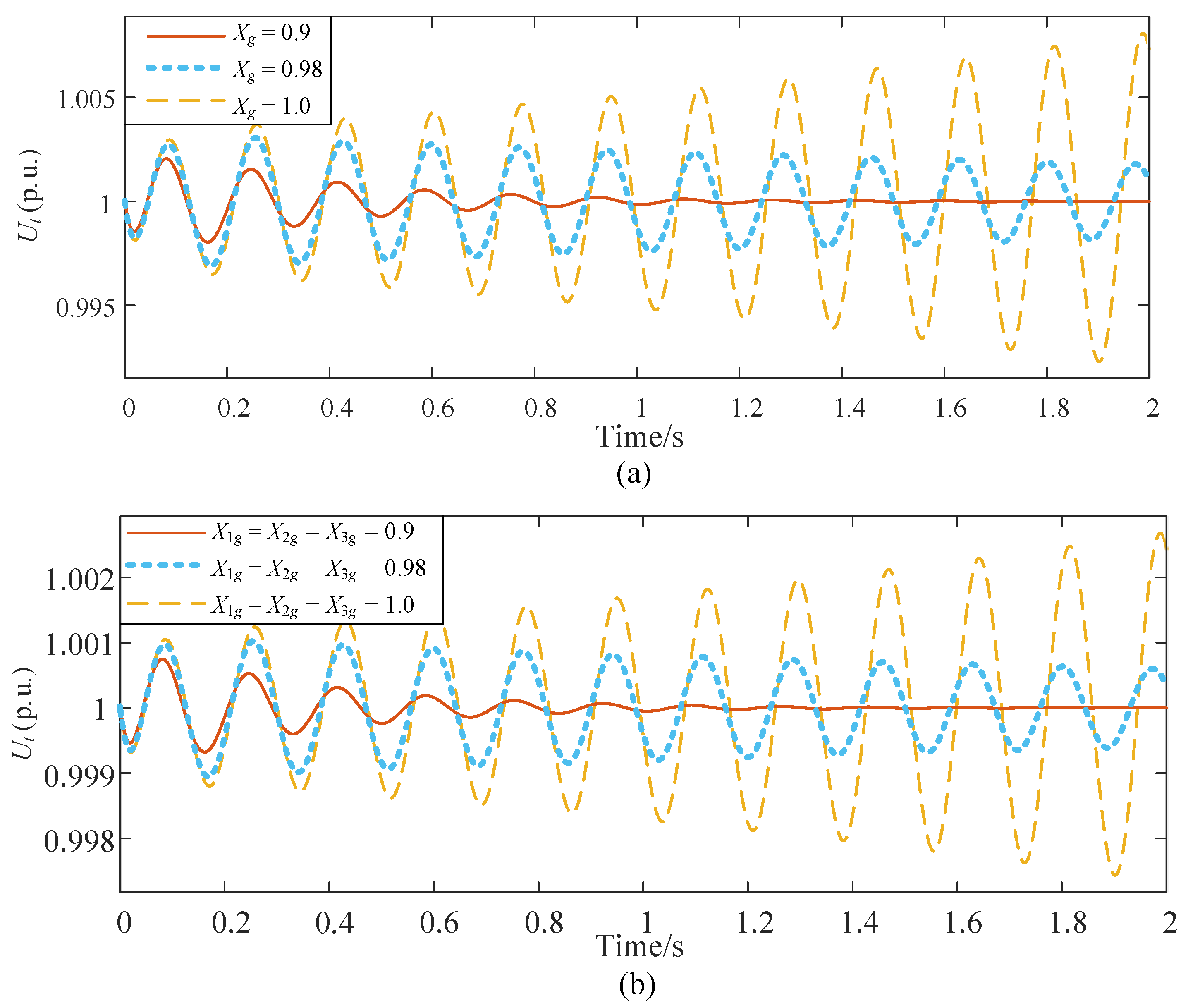
5.3. Time-Domain Simulation Results

To verify the above small-signal stability analysis results, sufficient time-domain simulations on the original nonlinear system were conducted in the MATLAB/Simulink. The controller parameters used are listed in the Appendix A. First, the single-VSC system in Figure 6 is studied with the identical device parameters. Three tests for different VSC-grid reactances, including $X_g=0.9$, $X_g=0.98$, and $X_g=1.0$ were conducted. A small step disturbance of amplitude, $0.01$ p.u., was added on $i_{d0}$ at the beginning, which indicates that there is a small node injection current disturbance. The corresponding three terminal voltages of VSC are shown in Figure 11a, where the three curves are for stable, critical stable, and unstable behaviors, respectively. The occurrence of a critical VSC-grid reactance at $X_{g,c}\approx 0.98$ in the plots is in accordance with the eigenvalue analysis in Figure 8 before.

For comparison, a three-VSC system has been studied. As the condition for identical VSC-grid reactances is necessary in our theory, we consider $X_{1g}=X_{2g}=X_{3g}=0.9$, $X_{1g}=X_{2g}=X_{3g}=0.98$, and $X_{1g}=X_{2g}=X_{3g}=1.0$, corresponding to the above three cases of a single-VSC system. The other parameters for the inter-VSC reactances $X_{12}=0.5$, $X_{13}=0.2$, and $X_{23}=0.8$ has been arbitrarily chosen. The same disturbance is given to one VSC, with its corresponding terminal voltage waveform shown in Figure 11b. Comparing these two panels in Figure 11, one can clearly see that the critical VSC-grid reactance in the multi-converter system is nearly unchanged; $X_{g,c}\approx 0.98$. This again demonstrates that the whole large-scale system dynamics is indeed solely described by only one dominant subsystem with the key parameter $X_g$.

6. Conclusions

In conclusion, we have developed an appropriate theory for the small-signal stability in multi-converter systems, from nonlinear modeling to linear modeling and its approximation, based on three important techniques: multi-timescale decomposition, linearization, and symmetry decoupling. We have found that, under the approximation assumptions, the whole huge system can be well-decomposed into several subsystems and each subsystem can be treated as a single-converter system with an effective network susceptance. The stability of the large-scale multi-converter system is determined by only one dominant subsystem, whose network parameter is equal to the original converter-grid susceptance.

Essentially, the key to decouple the multi-machine power system into several single-machine systems is to decouple the power network, which is often represented by the admittance matrix in the mathematical model. The matrix itself has a natural symmetry. Only when the matrix of each device connected in the network does not destroy this symmetry, the characteristic matrix of the whole system keeps symmetric and then we can decouple the power system. Therefore, we put forward strict conditions for the device and network in this paper to meet the requirement of precise decoupling. However, when the parameters of the device or network appear little deviation or the power flow in the network is not obviously asymmetric, the decoupling condition may be relaxed, so that it can be better applied and popularized in real scenes. We believe that this theory provides a theoretical tool for analyzing integrated renewable power systems and helps to find the key transmission lines.

On the other hand, as is known, the multi-converter system is also a typical networked dynamical system consisting of dynamical nodes and a stationary network. Possible methods and techniques from relevant disciplines, such as complex systems, nonlinear dynamics, and statistical mechanics as well, are highly appreciated. Different from the well studied synchronization process in traditional power grids, the physical mechanism of the power-electronic-based power grid remains obscure. We hope that our paper could fill the gap between power electrical engineering and contemporary physics by a clear description of modeling details of power electronic devices. It could arouse extensive interests among physicists with network dynamics background for further investigations.

References

1. Blaabjerg, F.; Ma, K. Future on power electronics for wind turbine systems. IEEE J. Emerg. Select. Top. Power Electr. 2013, 1, 139–152. [Google Scholar] [CrossRef]
2. Wang, X.; Blaabjerg, F. Harmonic stability in power electronic-based power systems: Concept, modeling, and analysis. IEEE Trans. Smart Grid 2018, 10, 2858–2870. [Google Scholar] [CrossRef] [Green Version]
3. Veers, P.; Dykes, K.; Lantz, E.; Barth, S.; Bottasso, C.L.; Carlson, O.; Clifton, A.; Green, J.; Green, P.; Holttinen, H.; et al. Grand challenges in the science of wind energy. Science 2019, 366, eaau2027. [Google Scholar] [CrossRef] [PubMed] [Green Version]
4. Kundur, P.; Balu, N.J.; Lauby, M.G. Power System Stability and Control; McGraw-hill New York: New York, NY, USA, 1994; Volume 7. [Google Scholar]
5. Anderson, P.M.; Fouad, A.A. Power System Control and Stability; John Wiley & Sons: Hoboken, NJ, USA, 2008. [Google Scholar]
6. Ni, Y.; Chen, S.; Zhang, B. Theory and Analysis of Dynamic Power System; Tsinghua University Publication: Beijing, China, 2002. (In Chinese) [Google Scholar]
7. Zhao, M.; Yuan, X.; Hu, J.; Yan, Y. Voltage dynamics of current control time-scale in a VSC-connected weak grid. IEEE Trans. Power Syst. 2015, 31, 2925–2937. [Google Scholar] [CrossRef]
8. Wang, Y.; Wang, X.; Chen, Z.; Blaabjerg, F. Small-signal stability analysis of inverter-fed power systems using component connection method. IEEE Trans. Smart Grid 2017, 9, 5301–5310. [Google Scholar] [CrossRef] [Green Version]
9. Yang, Z.; Ma, R.; Cheng, S.; Zhan, M. Nonlinear Modeling and Analysis of Grid-connected Voltage Source Converters Under Voltage Dips. IEEE J. Emerg. Select. Top. Power Electr. 2020, 8, 3281–3292. [Google Scholar] [CrossRef]
10. Yang, Z.; Ma, R.; Cheng, S.; Zhan, M. Problems and Challenges of Power-electronic-based Power System Stability: A Case Study of Transient Stability Comparison. Acta Phys. Sin. 2020, 69, 1–14. [Google Scholar]
11. Yang, Z.; Mei, C.; Cheng, S.; Zhan, M. Comparison of Impedance Model and Amplitude-Phase Model for Power-electronics-based Power System. IEEE J. Emerg. Select. Top. Power Electr. 2019, 8, 2546–2558. [Google Scholar] [CrossRef]
12. Ji, Y.; He, W.; Cheng, S.; Kurths, J.; Zhan, M. Dynamic network characteristics of power-electronics-based power Systems. Sci. Rep. 2020, 10, 1–16. [Google Scholar] [CrossRef]
13. Qiu, Q.; Zhou, B.; Wang, P.; He, L.; Xiao, Y.; Yang, Z.; Zhan, M. Origin of amplitude synchronization in coupled nonidentical oscillators. Phys. Rev. E 2020, 101, 022210. [Google Scholar] [CrossRef]
14. Beerten, J.; D’Arco, S.; Suul, J.A. Identification and small-signal analysis of interaction modes in VSC MTDC systems. IEEE Trans. Power Deliv. 2015, 31, 888–897. [Google Scholar] [CrossRef] [Green Version]
15. Hu, J.; Yuan, X.; Cheng, S. Multi-time scale transients in power-electronized power systems considering multi-time scale switching control schemes of power electronics apparatus. Proc. Chin. Soc. Elect. Eng. 2019, 39, 5457–5467. [Google Scholar]
16. Wang, L.; Xie, X.; Liu, H.; Zhan, Y.; He, J.; Wang, C. Review of emerging SSR/SSO issues and their classifications. J. Eng. 2017, 2017, 1666–1670. [Google Scholar] [CrossRef]
17. Xie, X.; Wang, L.; He, J.; Liu, H.; Wang, C.; Zhan, Y. Analysis of subsynchronous resonance/oscillation types in power systems. Power Syst. Technol. 2017, 41, 1043–1049. [Google Scholar]
18. Wang, X.; Du, W.; Wang, H. Stability analysis of grid-tied VSC systems under weak connection conditions. Proc. CSEE 2018, 26, 1593–1604. [Google Scholar]
19. Huang, Y.; Zhai, X.; Hu, J.; Liu, D.; Lin, C. Modeling and stability analysis of VSC internal voltage in DC-link voltage control timescale. IEEE J. Emerg. Select. Top. Power Electr. 2017, 6, 16–28. [Google Scholar] [CrossRef]
20. Zhu, J.; Hu, J.; Lin, L.; Wang, Y.; Wei, C. High-Frequency Oscillation Mechanism Analysis and Suppression Method of VSC-HVDC. IEEE Trans. Power Electr. 2020, 35, 8892–8896. [Google Scholar] [CrossRef]
21. Barrat, A.; Barthelemy, M.; Vespignani, A. Dynamical Processes on Complex Networks; Cambridge University Press: Cambridge, UK, 2008. [Google Scholar]
22. Menck, P.J.; Heitzig, J.; Marwan, N.; Kurths, J. How basin stability complements the linear-stability paradigm. Nat. Phys. 2013, 9, 89–92. [Google Scholar] [CrossRef] [Green Version]
23. Menck, P.J.; Heitzig, J.; Kurths, J.; Schellnhuber, H.J. How dead ends undermine power grid stability. Nat. Commun. 2014, 5, 1–8. [Google Scholar] [CrossRef]
24. Nitzbon, J.; Schultz, P.; Heitzig, J.; Kurths, J.; Hellmann, F. Deciphering the imprint of topology on nonlinear dynamical network stability. New J. Phys. 2017, 19, 033029. [Google Scholar] [CrossRef]
25. Rohden, M.; Sorge, A.; Timme, M.; Witthaut, D. Self-organized synchronization in decentralized power grids. Phys. Rev. Lett. 2012, 109, 064101. [Google Scholar] [CrossRef] [PubMed] [Green Version]
26. Yang, Y.; Nishikawa, T.; Motter, A.E. Small vulnerable sets determine large network cascades in power grids. Science 2017, 358. [Google Scholar] [CrossRef] [PubMed] [Green Version]
27. Schäfer, B.; Witthaut, D.; Timme, M.; Latora, V. Dynamically induced cascading failures in power grids. Nat. Commun. 2018, 9, 1–13. [Google Scholar] [CrossRef] [PubMed]
28. Witthaut, D.; Timme, M. Braess’s paradox in oscillator networks, desynchronization and power outage. New J. Phys. 2012, 14, 083036. [Google Scholar] [CrossRef]
29. Motter, A.E.; Myers, S.A.; Anghel, M.; Nishikawa, T. Spontaneous synchrony in power-grid networks. Nat. Phys. 2013, 9, 191–197. [Google Scholar] [CrossRef] [Green Version]
30. Barzel, B.; Barabási, A.L. Universality in network dynamics. Nat. Phys. 2013, 9, 673–681. [Google Scholar] [CrossRef] [Green Version]
31. Wolff, M.F.; Schmietendorf, K.; Lind, P.G.; Kamps, O.; Peinke, J.; Maass, P. Heterogeneities in electricity grids strongly enhance non-Gaussian features of frequency fluctuations under stochastic power input. Chaos Interdiscipl. J. Nonlinear Sci. 2019, 29, 103149. [Google Scholar] [CrossRef]
32. Timme, M.; Kocarev, L.; Witthaut, D. Focus on networks, energy and the economy. New J. Phys. 2015, 17, 110201. [Google Scholar] [CrossRef]
33. Ongena, J. Focus Point on the Transition to Sustainable Energy Systems. Eur. Phys. J. Plus 2018, 133, 82. [Google Scholar] [CrossRef] [Green Version]
34. Anvari, M.; Hellmann, F.; Zhang, X. Introduction to Focus Issue: Dynamics of modern power grids. Chaos Interdiscipl. J. Nonlinear Sci. 2020, 30, 063140. [Google Scholar] [CrossRef]
35. Ma, Y.; Yang, P.; Wang, Y.; Zhao, Z. Typical characteristics and key technologies of microgrid. Autom. Electr. Power Syst. 2015, 39, 168–175. [Google Scholar]
36. Pérez-Collazo, C.; Greaves, D.; Iglesias, G. A review of combined wave and offshore wind energy. Renew. Sustain. Energy Rev. 2015, 42, 141–153. [Google Scholar] [CrossRef] [Green Version]
37. Shalwala, R.; Bleijs, J. Impact of Grid-Connected PV systems on voltage regulation of a residential area network in Saudi Arabia. In Proceedings of the IEEE 2010 1st International Nuclear & Renewable Energy Conference (INREC), Amman, Jordan, 21–24 March 2010; pp. 1–5. [Google Scholar]
38. Du, W.; Fu, Q.; Wang, X.; Wang, H. Small-signal stability analysis of integrated VSC-based DC/AC power systems—A review. Int. J. Electr. Power Energy Syst. 2018, 103, 545–552. [Google Scholar] [CrossRef]
39. Bahirat, H.J.; Mork, B.A.; Høidalen, H.K. Comparison of wind farm topologies for offshore applications. In Proceedings of the IEEE 2012 Power and Energy Society General Meeting, San Diego, CA, USA, 22–26 July 2012; pp. 1–8. [Google Scholar]
40. Wu, B.; Narimani, M. High-Power Converters and AC Drives; John Wiley & Sons: Hoboken, NJ, USA, 2017. [Google Scholar]
41. Ackermann, T. Wind Power in Power Systems; John Wiley & Sons: Hoboken, NJ, USA, 2005. [Google Scholar]
42. Jovcic, D. High Voltage Direct Current Transmission: Converters, Systems and DC Grids; John Wiley & Sons: Hoboken, NJ, USA, 2019. [Google Scholar]
43. Nilsson, J.W. Electric Circuits; Pearson Education India: Chennai, India, 2008. [Google Scholar]
44. Horn, R.A.; Johnson, C.R. Matrix Analysis; Cambridge University Press: Cambridge, UK, 2012. [Google Scholar]
Figure 1. The offshore wind farm with wind turbines connecting each other is known as a collection system and then it is connected to the onshore grid usually by a high voltage transmission system. The collection system topologies can be radical connection (a), radical loop connection (b), and star connection (c).
Symmetry 13 00157 g001
Figure 2. (a) Topological structure for a multi-voltage source converter (VSC) infeed system within the DC-link voltage timescale, with each VSC connected to an infinitely strong bus U t , n + 1 . We use X i j and X i g to denote the inter-converter and converter-grid reactances, respectively. X i j = X j i and X i g = X g i . (b) Equivalent circuit topology of (a), where each VSC serves as a controlled current source and injects power to the network.
Symmetry 13 00157 g002
Figure 3. Control diagram of a multi-VSC power system with typical cascade vector controllers, including the terminal voltage control loop (TVC) and DC voltage control loop (DVC) for the outer slow-scale controls, and the AC current control loop (ACC) for the inner fast-scale control. The phase-locked control loop (PLL) is used for synchronization, by inputting the terminal voltage angle θ t , i and outputting the phase-locked angle θ i . The PLL also belongs to the DVC timescale and will be included in our model. All controllers including the TVC, DVC, and ACC are designed depending on the PLL reference frame.
Symmetry 13 00157 g003
Figure 4. (a) Schematic show for the x y synchronous reference coordinate and the d q PLL coordinate used in the multi-converter system. The x y rotates at a fixed speed ω 0 . In contrast, the d q coordinate is based on the phase-locked angle θ i (from the terminal voltage phase angle θ t , i ) and implements the cascade vector control. Its speed ω p l l , i is time-varying. (b) Similar to (a) but for a synchronous generator. Similarly, the x y frame rotates at a fixed speed ω 0 and the d q frame rotates at the rotor speed ω i , which is also time-varying. δ i denotes the power angle and θ t , i is the terminal voltage phase angle. In a traditional power system, the dynamics of δ i of the synchronous generator (SG) plays a key role in the system electromechanical behavior, similar to the phase-locked angle θ i in the PLL in (a).
Symmetry 13 00157 g004
Figure 5. Diagram of a multi-VSC power system within the DC voltage time-scale, including the detailed TVC, DVC, and PLL controllers. The control goals of the TVC and DVC are to maintain the terminal voltage and DC voltage at normal values, respectively. As the dynamic of ACC has been ignored, the VSC is recognized as a controlled current source. d t presents an integral of the input.
Symmetry 13 00157 g005
Figure 6. Schematic show for a single VSC infeed system.
Symmetry 13 00157 g006
Figure 7. Flow chart of the conclusion derivation.
Symmetry 13 00157 g007
Figure 8. Root loci of the single-VSC infeed system with the converter-grid reactance X g varying from 0.1 (circle) to 1.1 (star). In particular, a critical reactance X g , c exists; X g , c 0.98 . For X g > X g , c , the system becomes unstable.
Symmetry 13 00157 g008
Figure 9. Comparison of the numerical root loci of the three-VSC infeed system in (a) and its three theoretical decoupled subsystems in (bd), based on the three estimated effective converter-grid inductance B e 1 , B e 2 , B e 3 correspondingly. For the parameters, we fix X g = 0.5 , X 13 = 0.2 , and X 23 = 0.8 , but change X 12 from 0.1 (circle) to 1.1 (star).
Symmetry 13 00157 g009
Figure 10. Comparison of the numerical root loci of the three-VSC infeed system in (a) and its three theoretical decoupled subsystems in (bd), based on the three estimated effective converter-grid inductance B e 1 , B e 2 , B e 3 correspondingly. Similar to Figure 9, but for another parameter test, instead. Now we fix X 12 = X 23 = X 13 = 0.5 and change X g from 0.1 (circle) to 1.1 (star).
Symmetry 13 00157 g010
Figure 11. Time-domain simulation results for the single-VSC infeed system (a) and the three-VSC infeed system (b). Both cases show that the critical reactance X g is 0.98 . In (b), for other parameters, X 12 = 0.5 , X 13 = 0.2 , and X 23 = 0.8 are arbitrarily chosen.
Symmetry 13 00157 g011
Publisher’s Note: MDPI stays neutral with regard to jurisdictional claims in published maps and institutional affiliations.