A Novel Model for Distributed Denial of Service Attack Analysis and Interactivity

Abstract

A Distributed Denial of Service (DDoS) attack is a type of cybercrime that renders a target service unavailable by overwhelming it with traffic from several sources (attack nodes). In this paper, we focus on DDoS attacks on a computer network by spreading bots throughout the network. A mathematical differential equation model is proposed to represent the dynamism of nodes at different compartments of the model. The model considers two levels of security, with the assumption that the recovered nodes do not return to the same security level. In previous models, the recovered nodes are returned to be suspect on the same security level, which is an unrealistic assumption. Moreover, it is assumed that the attacker can use the infected target nodes to attack again. With such epidemic-like assumptions of infection, different cases are presented and discussed, and the stability of the model is analyzed as well; reversing the symmetry transformation of attacking nodes population is also proven. The proposed model has many parameters in order to precisely describe the infection movement and propagation. Numerical simulation methods are used to solve the developed system of equations using MATLAB, with the intention of finding the best counteraction to control DDoS spread throughout a network.

1. Introduction

A Denial of Service attack (DoS attack) is a cyberattack in which the attacker attempts to reduce the access or completely shut down the resources of either a machine or a network and make them unavailable to their legitimate users [1]. The DoS attack has been known to the scientific community since the early 1980s. In 1983, Gligor provided one of the first descriptions of a DoS attack in an operating system [1].

A Distributed Denial of Service (DDoS) attack is a large-scale DoS attack in which the attacking system consists of a large number of compromised computers that are targeting the victim’s system. Usually, a DDoS attack consists of two stages; in the first stage, the attacking system compromises a large number of vulnerable computers in order to use them as a part of the attacking attempt during the second stage, wherein the victim’s system is attacked.

A famous example was in July 2001, when more than 350,000 computers were infected with the Code Red worm in less than 14 h. Then, the worm attempted to launch a DDoS attack against the White House website. However, it was easy to disable the second stage of the attack due to its features [2].

An example of a DoS attack is the SYN flood attack in which the attacker exploits part of the Transmission Control Protocol (TCP), specifically, the handshake process. TCP is a host-to-host communication protocol designed to send data packets over the Internet. In this attack, the attacking system repeatedly sends SYN packets to the victim’s system without responding to the SYN/ACK packets sent by the server. Thus, the connection remains in a half-open state, and due to a large number of connections, the victim’s system cannot respond to any new connection. One of the early SYN flood attacks occurred in September 1996, when an attacker shut down the New York City Internet service provider, Panix, for almost a week [3]. In the first quarter of 2018, 57.3% of DDoS attacks were SYN flood attacks [4].

Another protocol that can be misused to attack the victim’s system is the Internet Control Message Protocol (ICMP). ICMP is a supporting protocol that is used to send error messages and operational information. In the first quarter of 2018, 6.1% of DDoS attacks were ICMP attacks [4]. An example of ICMP flooding attacks is the ping flooding attack, which is one of the simplest DoS attacks. Ping is a computer network utility to test the reachability of a host on a particular Internet Protocol (IP) address. In the ping flooding attack, the attacking system repeatedly sends more ping packets than the victim’s system can handle.

In general, DoS attacks can be categorized into two types: crash the service or flood the service. In the “crash the service” attack, the attacking system aims to crash or freeze the victim’s system by exploiting a software vulnerability it has. On the other hand, the “flood the service” attack aims to flood the victim’s system with useless traffic in order to overload the system and prevent the legitimate traffic from being served [5].

DDoS attacks can be very dangerous and may cause serious damage. In February 2000, Yahoo, Buy.com, eBay, CNN.com, Amazon.com, Dell, ZDNet, E*Trade, and Excite were targets of a 15-year-old Canadian nicknamed “Mafiaboy” [6,7]. The estimated damages of the attack were $1.7 billion [8].

Another example is Dyn, an Internet performance management and web application security company that was compromised in October 2016. During this time, their Managed Domain Name System (DNS) infrastructure came under two DDoS attacks [9]. These attacks were caused by up to 100,000 malicious endpoints in which a large amount of the traffic originated from Mirai-based botnets [9]. Websites such as Twitter, Spotify, PayPal, HSBC, BankWest, and Ticketmaster suffered from connectivity problems [10]. As a result, 8% of Dyn’s customers dropped the company as their DNS service provider [10].

The concept of symmetry is one of the important things that is closely related to systems of differential equations in the theory of dynamical systems. This correlation was discussed in [11,12,13]. According to [14], considering an autonomous dynamical system of differential equation such as:

$$\frac{d\omega }{dt}=\mathcal{F}\left(\omega \right),$$

(1)

where $\omega \in {\mathbf{R}}^n$, and the transformation $\mathcal{T}:{\mathbf{R}}^n\to {\mathbf{R}}^n$ is a reversing symmetry of (1) if:

$$\frac{d}{dt}\left(\mathcal{T}\omega \right)=-\mathcal{F}\left(\mathcal{T}\omega \right),$$

(2)

In this case, system (2) is invariant with respect to the transformation $(t,\omega )\to (-t,\mathcal{T})$, which holds in our attack population study and is described in the numerical analysis section.

The problem of stability in dynamic systems is one of the fundamental problems in various fields of science and modern technology [15,16]. Because of its importance, the concept of symmetry and its impact on this work is referred to in the proposed study.

In this work, we use non-linear differential equation systems to describe and analyze DDoS attacks on highly protected systems, such as main enterprise servers, and poorly protected systems, such as normal users’ devices. We propose a new variable that illustrates the degree of protection among those different system types in order to study the different possible scenarios, which will lead to a more comprehensive description that covers the impact of such attacks on targeted networks. We also prove that depending on backup servers alone is not an efficient solution for this kind of attacks, but can actually complicate the problem and waste resources. The research also describes the botnet and its effect on the targeted devices, which is an important aspect of the work because we study both the attacking and the targeted societies. It is also significant to mention that our model is more realistic than others because the recovered nodes will have high-level security after the attack, which is an assumption that has usually been omitted in previous models. Moreover, this dynamical system of equation is generally much faster than botnet simulation, although the simulation is more accurate. Other techniques, such as machine learning, have been used to learn the behavior of DDoS and botnet; however, they do not give the analytical strength and dynamics of an equations model approach.

The rest of this paper is organized as follows: Background and relevant literature are presented in Section 2. The model formulation, design, and basic properties are introduced in Section 3. Section 4 presents the numerical analysis and discussion to approximate the solution and show the stability and comparison. Finally, Section 5 concludes the paper.

2. Background

DDoS, or Distributed Denial of Service, is a common cyberattack technique that hackers favor since it is not easy to counter, allows the attacker to remain undetected, and has a low attack cost [17]. In a typical Denial of Service (DoS) attack, attackers attempt to block one or more servers on the network from serving legitimate users. This type of assault is known as Distributed Denial of Service (DDoS) since it originates from multiple sources [18,19]. Attackers can infect a node by injecting a kind of Trojan horse, for example, in a variety of ways, including embedding it in free games or media downloads, or by attaching it to emails. The attacker then uses the injected code to interact with an external entity, which starts a massive attack on the victim’s nodes, preventing them from working and providing the necessary services correctly [20].

In DDoS, it is critical to look into the propagation characteristics of infection. Suspicious objects can easily spread throughout a network, posing a major security risk. Because the network infrastructure must be resistant to these attacks, the isolation of infected nodes is essential for avoiding the spread of the infection. Infected nodes are disconnected from the rest of the network until they can be recovered. So far, the containment strategy’s intervention has resulted in significant modifications in infection solutions, which have been fine tuned to protect systems from DDoS attacks. To comprehend and analyze these attacks, mathematical models have been developed [21]. Because infection via malicious objects is analogous to real diseases, the epidemic model has proven to be a valuable tool for understanding how they propagate throughout a computer network [22,23]. Epidemiological models are essentially dynamic since they divide the entire population of nodes into multiple compartments, such as infected, susceptible, or recovered [24]. Differential equations can describe the movement of a node from one compartment to another. This system is then examined to see whether or not stability has been achieved. Another advantage of such models is the inclusion of an epidemic threshold, which aids in determining whether the epidemic will persist or go away [25].

Several researchers have utilized mathematical techniques to create a model of the DDoS attack that can be investigated and analyzed. Mishra et al. [26] created a model to simulate a cyberattack on an IoT network based primarily on the Mirai botnet malware. They looked at the model’s equilibrium and stability and ran numerical simulations of several scenarios. The model was created to analyze a DDoS attack spread on a targeted network using a previously constructed IoT botnet and to explain the wireless transmission of attacks in a network that could create a zombie army. Zhang [27] used a game theory-based DDoS attack model to address some of the flaws in earlier assumptions, such as the idea that defenders will utilize a fixed-probability defending technique or that they will not adopt defense tactics because of defensive costs. Zhang [27] developed two smooth logistic functions to represent the defender’s defense strategy options under various cost-benefit scenarios in order to investigate the impact of defense strategy decisions on the dynamic behavior of DDoS attacks. They also used the theory of differential stability to find the attack threshold, which determines the conditions for a successful attack, and to prove the attack equilibrium and the attack-free equilibrium.

3. Model Formulation and Basic Properties

The model is designed by splitting the total network into attack and target populations at time t. The attack population has the following two compartments: a percentage of the susceptible, denoted by $S_a\left(t\right)$, and a percentage of the infectious, denoted by $I_a\left(t\right)$. Hence, the total percentage of this population is $S_a\left(t\right)+I_a\left(t\right)=1$.

On the other hand, we assumed that the target population was divided into two sub-populations, which are:

(i)

Low-security population, which has the following three compartments: a percentage of the susceptible, denoted by $S_l\left(t\right)$, a percentage of the infectious, denoted by $I_l\left(t\right)$, and a percentage of the recovered, denoted by $R_l\left(t\right)$;

(ii)

High-security population, which has the following three compartments: a percentage of the susceptible, denoted by $S_h\left(t\right)$, a percentage of the infectious, denoted by $I_h\left(t\right)$, and a percentage of the recovered, denoted by $R_h\left(t\right)$.

Therefore, the total percentage of this population is $S_l\left(t\right)+I_l\left(t\right)+R_l\left(t\right)+S_h\left(t\right)+I_h\left(t\right)+R_h\left(t\right)=1$.

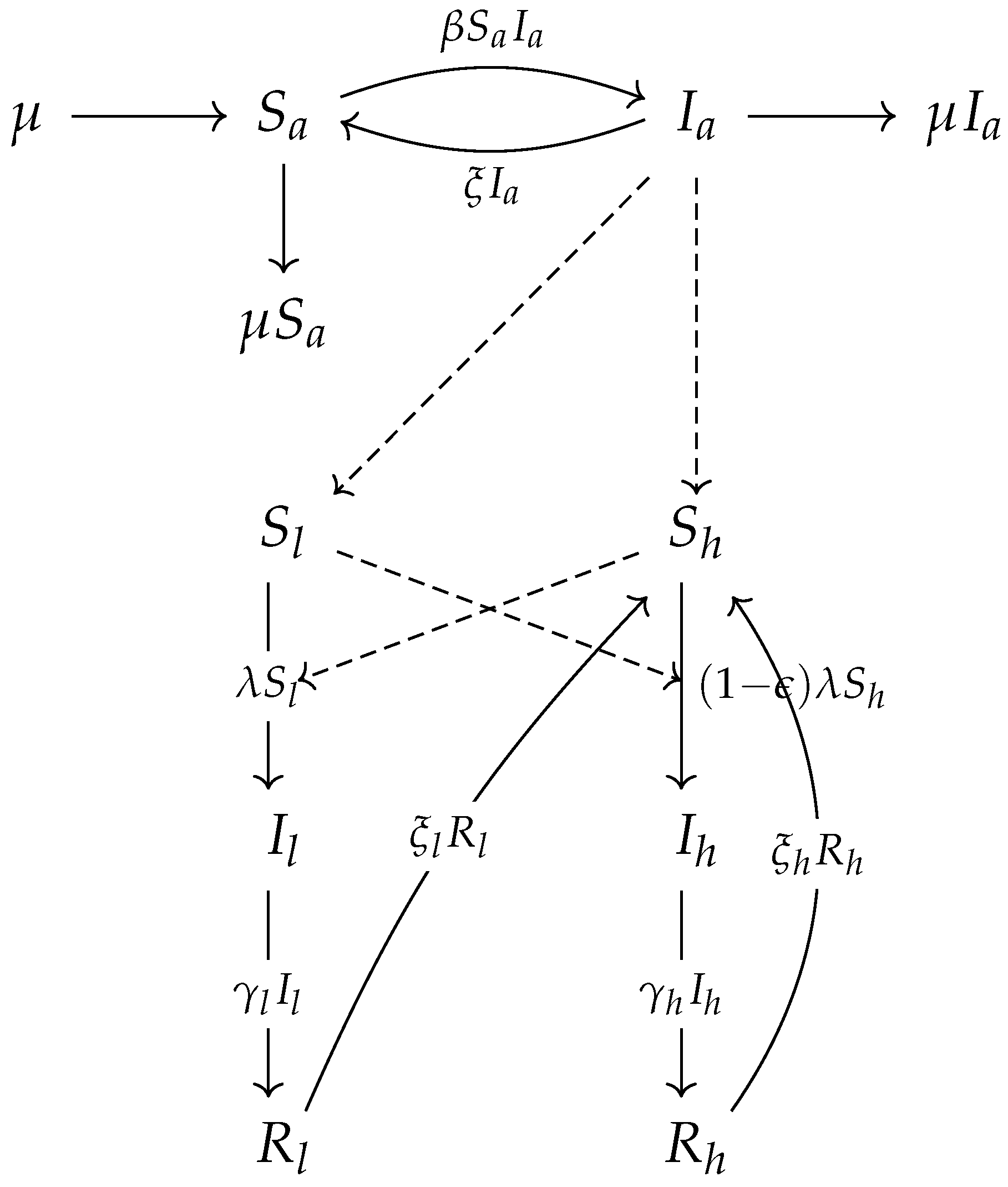
The equations of the model are obtained as follows: Nodes are recruited into the attack population at a rate $\mu$. Susceptible nodes of the attack population may be infected with infectious nodes at rate $\beta I$, in which $\beta$ is the effective contact rate. The attack population is decreased by natural death, $\mu$, and the recovery rate of target population nodes that become suspicious again is $\xi$. Thus, the changing rate of the attack population for both susceptible and infected nodes are given, respectively, by the following:

$$\begin{array}{cc}\hfill \frac{d{S}_a}{dt}& =\mu -\beta S_a{I}_a-\mu S_a+\xi I_a,\hfill \\ \hfill \frac{d{I}_a}{dt}& =\beta S_a{I}_a-(\xi +\mu )I_a.\hfill \end{array}$$

(3)

Lemma 1.

The transformation $\mathcal{T}:{\mathbf{R}}^n\to {\mathbf{R}}^n$ is a reversing symmetry for an invariable attack population, without disconnected nodes.

Proof. 

$\mu =0$ since the population is invariable, and all nodes are connected for the run time of the DDoS attack. Now, by letting $(t,\mathbf{x})\to (-t,\mathcal{T}\mathbf{x})$ for $\mathbf{x}=(S_a,I_a)$, where $\mathcal{T}(S_a,I_a)=(I_a,S_a)$, then the proof of the lemma can clearly be concluded. □

Target susceptible nodes may be infected at rate $\lambda$:

$$\lambda =\beta \left[I_a+\eta (I_h+I_l)\right],$$

(4)

where $\eta$ is the modification parameter which accounts for the attack transmission of the infected target nodes for the assumed reduction (in the $I_l$ and $I_h$ compartments). Furthermore, the infected nodes are recovered at a rate ${\gamma }_l$, and the recovered nodes are fortified at a rate ${\xi }_l$ in order to become suspect at a high-security level.

Thus, the changing rate of the low-security population of the susceptible, infected, and recovered nodes are given, respectively, by the following:

$$\begin{array}{cc}\hfill \frac{d{S}_l}{dt}& =-\lambda S_l,\hfill \\ \hfill \frac{d{I}_l}{dt}& =\lambda S_l-{\gamma }_l{I}_l,\hfill \\ \hfill \frac{d{R}_l}{dt}& ={\gamma }_l{I}_l-{\xi }_l{R}_l.\hfill \end{array}$$

(5)

It is further assumed that the high-security level is imperfect, so that the high-security susceptible nodes may be infected at a reduced rate $(1-ϵ)\lambda$, in which $ϵ$ represents the firewall efficiency.

Additionally, the infected nodes are recovered at a rate ${\gamma }_h$, then these recovered nodes may be infected again at a rate ${\xi }_h$.

Thus, the changing rate of the low-security population of the susceptible, infected, and recovered nodes are given, respectively, by the following equations:

$$\begin{array}{cc}\hfill \frac{d{S}_h}{dt}& =-\lambda (1-ϵ)S_h+{\xi }_h{R}_h+{\xi }_l{R}_l,\hfill \\ \hfill \frac{d{I}_h}{dt}& =\lambda (1-ϵ)S_h-{\gamma }_h{I}_h,\hfill \\ \hfill \frac{d{R}_h}{dt}& ={\gamma }_h{I}_h-{\xi }_h{R}_h.\hfill \end{array}$$

Combining the aforementioned derivations and assumptions, the model of the DDoS attack on a computer network is expressed in the following equations, model (6), with a schematic presentation in Figure 1, and a description of the parameters in

Table 1. Description of the system’s parameters (6).

Parameter	Description
$\mu$	recruitment rate
$\eta$	modification parameter that accounts for the attack
	transmission of the infected target nodes for the assumed
	reduction (in the $I_l,I_h$ compartments)
$\beta$	effective contact rate
${\beta }_h$	effective contact rate of the high-security population
${\beta }_l$	effective contact rate of the low-security population
${\gamma }_h$	rate of recovered high-security infected nodes
${\gamma }_l$	rate of recovered low-security infected nodes
$\xi$	recovery rate of target population nodes that become suspicious again
${\xi }_h$	rate of recovered high-security nodes that become infected again
${\xi }_l$	rate of recovered low-security nodes that become infected again
$ϵ$	rate of firewall efficiency

.

$$\begin{array}{cc}\hfill \frac{d{S}_a}{dt}& =\mu -\beta S_a{I}_a-\mu S_a+\xi I_a,\hfill \\ \hfill \frac{d{I}_a}{dt}& =\beta S_a{I}_a-(\xi +\mu )I_a,\hfill \\ \hfill \frac{d{S}_l}{dt}& =-\lambda S_l,\hfill \\ \hfill \frac{d{I}_l}{dt}& =\lambda S_l-{\gamma }_l{I}_l,\hfill \\ \hfill \frac{d{R}_l}{dt}& ={\gamma }_l{I}_l-{\xi }_l{R}_l,\hfill \\ \hfill \frac{d{S}_h}{dt}& =-\lambda (1-ϵ)S_h+{\xi }_h{R}_h+{\xi }_l{R}_l,\hfill \\ \hfill \frac{d{I}_h}{dt}& =\lambda (1-ϵ)S_h-{\gamma }_h{I}_h,\hfill \\ \hfill \frac{d{R}_h}{dt}& ={\gamma }_h{I}_h-{\xi }_h{R}_h.\hfill \end{array}$$

(6)

The threshold value ${\mathcal{R}}_0$ can be defined as the average number of secondary infection nodes that a single infectious node can produce in a totally susceptible population. We first obtain the basic reproduction number separately for each population. The value of ${\mathcal{R}}_0$ for the target high-security population, denoted by $R_{0h}$, is defined as follows:

$$\begin{array}{c}\hfill R_{0h}=\frac{\beta (1-ϵ)}{{\gamma }_h},\end{array}$$

and for the target low-security population, we have:

$$\begin{array}{c}\hfill R_{0l}=\frac{\beta }{{\gamma }_l},\end{array}$$

and for the attack population, we have:

$$\begin{array}{c}\hfill R_{0a}=\frac{\beta }{\xi +\mu },\end{array}$$

By combining these values, we can get a single threshold value as in the host–vector models in epidemiology with the use of the notation in [28]. The non-negative matrix, $\mathcal{F}$, of the new infection terms, and the $\mathcal{V}$-matrix of the transition terms associated with model (6) are given, respectively, by the following equations:

$$\begin{array}{cc}\mathcal{F}=\left(\begin{array}{c}\lambda (1-ϵ)S_h\\ \lambda S_l\\ \beta S_a{I}_a\end{array}\right)& \mathrm{and}\mathcal{V}=\left(\begin{array}{c}{\gamma }_h{I}_h\\ {\gamma }_l{I}_l\\ (\xi +\mu )I_a,\end{array}\right)\end{array}$$

the corresponding derivative of the two vector-valued functions, $\mathcal{F}$ and $\mathcal{V}$, are the following:

$$\begin{array}{cc}F=\left(\begin{array}{ccc}-\beta \left(ϵ-1\right)& -\beta \eta \left(ϵ-1\right)& -\beta \eta \left(ϵ-1\right)\\ \beta & \beta \eta & \beta \eta \\ 0& 0& \beta \end{array}\right)& \mathrm{and}V=\left(\begin{array}{ccc}{\gamma }_h& 0& 0\\ 0& {\gamma }_l& 0\\ 0& 0& \mu +\xi \end{array}\right)\end{array}$$

It then follows that the control reproduction number [29], denoted by $\rho \left(F{V}^{-1}\right),$ in which

$$F{V}^{-1}=\left(\begin{array}{ccc}\frac{\beta (1-ϵ)}{{\gamma }_h}& \frac{\beta \eta (1-ϵ)}{{\gamma }_l}& \frac{\beta \eta (1-ϵ)}{\mu +\xi }\\ \frac{\beta }{{\gamma }_h}& \frac{\beta \eta }{{\gamma }_l}& \frac{\beta \eta }{\mu +\xi }\\ 0& 0& \frac{\beta }{\mu +\xi }\end{array}\right),$$

$\rho$ is defined as the spectral radius (maximum eigenvalue) of $F{V}^{-1}$, is given by

$$\begin{array}{cc}\hfill {\mathcal{R}}_0& =\rho \left(F{V}^{-1}\right)=max\{\frac{\beta }{\mu +\xi },\frac{\beta (1-ϵ)}{{\gamma }_h}+\frac{\beta }{{\gamma }_l}\}\hfill \\ & =max\{R_{0a},R_{0h}+R_{0l}\}.\hfill \end{array}$$

In the next subsection, the stability of the DDoS model is introduced. Moreover, it is shown that the threshold value $R_{0a}$ alone can completely determine the overall dynamics of the model (6), and there is no need to consider the value of ${\mathcal{R}}_0$. On the other hand, if we have a perfect security level ($ϵ=1$), then the attack effect will disappear with time.

3.1. Local Stability of Infection-Free Equilibrium

In this subsection, we will investigate the stability of the proposed model (6). Furthermore, we will analyze the effect of the firewall efficiency at the high-security level $ϵ$. The free infection point of model (6) is as follows:

$$P_0=(S_a^0,I_a^0,S_l^0,I_l^0,R_l^0,S_h^0,I_h^0,R_h^0)=(S_a^0,0,S_l^0,0,0,S_h^0,0,0),$$

in which $S_a^0=1$ and $S_l^0+S_h^0=1.$ The variables $(S_a,I_a,S_l,I_l,R_l,S_h,I_h,R_h)$ of model (6) are non-negative with time. In other words, the solutions of the model (6) system with positive initial data will remain positive at time t. This finding is shown in Theorem 1.

Theorem 1.

The closed set $D=\{x=(S_a,I_a,S_l,I_l,R_l,S_h,I_h,R_h)\in R_{+}^8:x_i\ge 0,S_a+I_a\le 1\mathit{and}{S}_l+I_l+R_l+S_h+I_h+R_h\le 1\}$ is positive invariant.

The proposed model (see Figure 1), given by model (6), is locally asymptotically stable (LAS) at the infection-free equilibrium $P_0$ if ${\mathcal{R}}_0\le 1$, and unstable if ${\mathcal{R}}_0>1$.

The existence of endemic equilibria (that is, equilibria where the infected compartments of the model are non-zero) of model (6) is established. Let $P_{*}=(S_a^{*},I_a^{*},S_l^{\ast },I_l^{\ast },R_l^{\ast },S_h^{\ast },I_h^{\ast },R_h^{\ast })$ represent any arbitrary endemic equilibrium point of model (6). To simplify the proposed model, we can solve the system of the attack population by solving the first and second equations in model (6) and get the following:

$$\frac{d{I}_a}{dt}=\beta (1-I_a)I_a-(\xi +\mu )I_a \mathrm{and} S_a=1-I_a.$$

Hence, the solution is as follows:

$$\begin{array}{cc}\hfill I_a& =\frac{(\xi +\mu -\beta )exp\left[(\xi +\mu -\beta )(t-I_a\left(0\right))\right]}{\beta exp\left[(\xi +\mu -\beta )(t-I_a\left(0\right))\right]+1},\hfill \\ \hfill S_a& =1-\frac{(\xi +\mu -\beta )exp\left[(\xi +\mu -\beta )(t-I_a\left(0\right))\right]}{\beta exp\left[(\xi +\mu -\beta )(t-I_a\left(0\right))\right]+1},\hfill \end{array}$$

(7)

Since the formula we get is explicit, we can easily study the stability of the attack population by taking the limit of (7):

$$\begin{array}{cc}\hfill \underset{t\to \infty }{lim}\frac{(\xi +\mu -\beta )exp\left[(\xi +\mu -\beta )(t-I_a\left(0\right))\right]}{\beta exp\left[(\xi +\mu -\beta )(t-I_a\left(0\right))\right]+1}& =\frac{\beta -\xi -\mu }{\beta }\hfill \end{array}$$

(8)

$$\begin{array}{cc}& =I^{\ast },\hfill \end{array}$$

(9)

if $\xi +\mu -\beta <0.$

Furthermore, let

$$\begin{array}{c}\hfill {\lambda }^{\ast }=\beta (I_a^{\ast }+\eta (I_h^{\ast }+I_l^{\ast })).\end{array}$$

(10)

When ${\mathcal{R}}_0>1$, then for a long time t (as t goes to infinity), the low-security population will be $S_l^{\ast }=I_l^{\ast }=R_l^{\ast }=0$ (at endemic equilibria $P^{\ast }$), because the attack consumes all devices in the low-security population. On the other hand, the high-security population at the steady state of the system is the following:

$$I_h^{\ast }=\frac{{\xi }_h(1-ϵ){\lambda }^{\ast }}{{\lambda }^{\ast }(1-ϵ)({\gamma }_h+{\xi }_h)+{\xi }_h{\gamma }_h},$$

substitute model (6) in order to get:

$$\begin{array}{c}\hfill {\lambda }^{\ast }=\beta \left(I_a^{\ast }+\frac{\eta {\xi }_h(1-ϵ){\lambda }^{\ast }}{{\lambda }^{\ast }(1-ϵ)({\gamma }_h+{\xi }_h)+{\xi }_h{\gamma }_h}\right),\end{array}$$

(11)

rewrite (11) as the following:

$$\begin{array}{c}\hfill a{\lambda }^{\ast 2}+b{\lambda }^{\ast }+c=0,\end{array}$$

(12)

in order to get:

$$\begin{array}{cc}\hfill & (1-ϵ)({\gamma }_h+{\xi }_h){\lambda }^{\ast 2}-\left[-{\xi }_h{\gamma }_h+\beta I_a^{\ast }({\gamma }_h+{\xi }_h)(1-ϵ)+\eta \beta {\xi }_h(1-ϵ)\right]{\lambda }^{\ast }-\beta {\xi }_h{\gamma }_h{I}_a^{\ast }=0,\hfill \end{array}$$

$$(1-ϵ)({\gamma }_h+{\xi }_h){\lambda }^{\ast 2}-\left[-{\xi }_h{\gamma }_h+[(\beta -\xi -\mu )({\gamma }_h+{\xi }_h)+\eta \beta {\xi }_h](1-ϵ)\right]{\lambda }^{\ast }-\beta {\xi }_h{\gamma }_h\left(1-\frac{1}{R_{0a}}\right)=0,$$

(13)

Based on (13), we can obtain the result in Theorem 2.

Theorem 2.

Model (6) has

• a unique endemic equilibrium if $c<0\iff R_{0a}>1$;
• a unique endemic equilibrium if $(b<0\mathit{and}c=0)\mathrm{or}{b}^2-4ac=0$;
• two endemic equilibria if $c>0,b<0\mathit{and}{b}^2-4ac>0$;
• no endemic equilibrium otherwise.

Case 1 shows that the model has a unique endemic equilibrium whenever $R_{0a}>1.$ While Case 3 shows that backward bifurcation is possible when

$$\begin{array}{c}\hfill {\mathcal{R}}_0^c=1-\frac{{[-{\xi }_h{\gamma }_h+\beta I_a^{\ast }({\gamma }_h+{\xi }_h)(1-ϵ)+\eta \beta {\xi }_h(1-ϵ)]}^2}{4(1-ϵ)({\gamma }_h+{\xi }_h)\beta {\xi }_h{\gamma }_h(1/R_{0h})},\end{array}$$

Backward bifurcation is where locally asymptotically stable infection-free equilibrium and locally asymptotically stable endemic equilibrium co-exist.

3.2. No High-Security Level

In this subsection, we will analyze the proposed model when $ϵ=0$ (if there is no high-security level, the firewall efficiency drops). In this case, the recovered nodes return to be infected again. But when $ϵ\ne 0$, the recovered nodes in the low-security level return to the S compartment in the high-security level.

If $ϵ=0$, we can conclude about parameters in the high-security population: the parameters in the target population are equal, i.e., ${\xi }_l={\xi }_h$ and ${\gamma }_l={\gamma }_h$, which means that the attack is equally effective on both low and high populations. The system of the target population becomes:

$$\begin{array}{cc}\hfill \frac{d{S}_t}{dt}& =-\lambda S_t+{\xi }_t{R}_t,\hfill \\ \hfill \frac{d{I}_t}{dt}& =\lambda S_t-{\gamma }_t{I}_t,\hfill \\ \hfill \frac{d{R}_t}{dt}& ={\gamma }_t{I}_t-{\xi }_t{R}_t,\hfill \end{array}$$

(14)

in which $\lambda =\beta (I_a+\eta I_t)$, $S_t=S_l+S_h,I_t=I_l+I_h$, and $R_t=R_l+R_h$. In addition, the system of the attack population is still the same:

$$\begin{array}{cc}\hfill \frac{d{S}_a}{dt}& =\mu -\beta S_a{I}_a-\mu S_a+\xi I_a,\hfill \\ \hfill \frac{d{I}_a}{dt}& =\beta S_a{I}_a-(\xi +\mu )I_a.\hfill \end{array}$$

The system is infection-free (weak attack) at $P_0=(1,0,1,0,0)$. The system is infected (successful attack) at the steady state, since $R_t=1-S_t-I_t$ and from the second equation of (system (14)):

$$\begin{array}{c}\hfill S_t=\frac{{\gamma }_t{I}_t}{\beta (I^{\ast }+\eta I_t)},\end{array}$$

(15)

substitute Equation (15) in the first equation of (14) to get the value of $I_t$, which is the positive solution of the following quadratic equation:

$$\begin{array}{c}\hfill -\beta \eta ({\gamma }_t+{\xi }_t)I_t^2-(\beta \eta +{\gamma }_t{\xi }_t+\beta I_a^{\ast }-{\xi }_t\beta )I_t+{\xi }_t\beta I_a^{\ast }=0\end{array}$$

(16)

Clearly, there is a unique positive solution for Equation (16) when $I_a^{\ast }\ne 0$ (infected solution), then $I_t^0$ is the positive solution of Equation (16). Therefore, $P^{\ast }=(S_a^{\ast },I_a^{\ast },S_t^{\ast },I_t^{\ast },R_t^{\ast })$ is the infected solution. It can be noticed that from Equation (16), if $I_a^{\ast }=0$, then $I_t^{\ast }=0$. Thus, the reproduction number is as follows:

$$\begin{array}{ccc}{\mathcal{R}}_0=max\left\{\frac{\beta }{{\gamma }_t},\frac{\beta }{\xi +\mu }\right\}& \mathrm{where}\frac{\beta }{{\gamma }_t}=R_{0t}& \mathrm{and}\frac{\beta }{\xi +\mu }=R_{0a}.\end{array}$$

Theorem 3.

The infection-free equilibrium $P_0$ of system (17) is locally asymptotically stable in D if ${\mathcal{R}}_0<1$ and is unstable if ${\mathcal{R}}_0>1$.

$$J\left(P_0\right)=\left[\begin{array}{ccc}-{\xi }_{\mathrm{t}}& -{\xi }_t-\beta \eta & -\beta \\ 0& \beta \eta -{\gamma }_t& \beta \\ 0& 0& \beta -\mu -\xi \end{array}\right],$$

(17)

in which J is the Jacobian matrix. The characteristic equation for this matrix is given as follows:

$$(\nu +{\xi }_t)(\nu -\beta \eta +{\gamma }_t)(\nu -\beta +\mu +\xi )=0$$

The roots of the characteristic equation are the eigenvalues of Equation (17), in which ${\nu }_1=-{\xi }_t$, ${\nu }_2=\beta \eta -{\gamma }_t$, and ${\nu }_3=\beta -(\mu +\xi )$. The second and third eigenvalues become negative when the following conditions are met: $\beta \eta -{\gamma }_t<0$ and $\beta -(\mu +\xi )<0$, which are equivalent to both $R_{0t}<1$ and $R_{0a}<1$, imply ${\mathcal{R}}_0<1$.

Theorem 4.

The infection-free equilibrium $P^{\ast }$ of system (18) is locally asymptotically stable if ${\mathcal{R}}_0>1$.

$$J\left(P^{\ast }\right)=\left[\begin{array}{ccc}-\beta (I^{\ast }+\eta I_t^{\ast })-{\xi }_t& -\beta \eta -{\xi }_t& -\beta S_t^{\ast }\\ \beta (I^{\ast }+\eta I_t^{\ast })& \beta \eta S^{\ast }-{\gamma }_t& \beta S_t^{\ast }\\ 0& 0& -2\beta I_a^{\ast }+\beta -(\xi +\mu )\end{array}\right],$$

(18)

One of the eigenvalues is $-2\beta I_a^{\ast }+\beta -(\xi +\mu )$, which is reduced to become $-(\beta -(\xi +\mu \left)\right)<0$, and is equivalent to $R_{0a}>1$. The other two eigenvalues are the roots of the characteristic equation of (17):

$${\nu }^2+[\beta (I_a^{\ast }+\eta I_t^{\ast })-\beta \eta S_t^{\ast }+{\gamma }_t]\nu +\beta (I_a^{\ast }+\eta I_t^{\ast })(-\beta \eta S_t^{\ast }+{\gamma }_t)+\beta (\beta +{\xi }_t)(I_a^{\ast }+\eta I_t^{\ast })=0.$$

(19)

To get the negative sum and the positive product of the roots in Equation (19), the following condition must be met: $-\beta \eta S_a^{\ast }+{\gamma }_t<0$, so, $1<{\displaystyle \frac{\beta \eta S_a^{\ast }}{{\gamma }_t}}<R_{0t}$.

Hence, the endemic equilibrium $P^{\ast }$ is locally asymptotically stable if ${\mathcal{R}}_0>1.$

Theorem 5.

The positive equilibrium point $P^{\ast }=(S_t^{\ast },I_t^{\ast },R_t^{\ast })$ is globally asymptotically stable whenever ${\mathcal{R}}_0>1$.

Proof. 

$$\begin{array}{cc}\hfill L(S_t,I_t)& =S_t-S_t^{\ast }ln{S}_t+I_t-I_t^{\ast }ln{I}_t\hfill \\ \hfill \frac{\partial L}{\partial t}& =S_t^{\prime }-\frac{S_t^{\ast }}{S_t}{S}_t^{\prime }+I_t^{\prime }-\frac{I_t^{\ast }}{I_t}{I}_t^{\prime }\hfill \\ \hfill & =-\lambda S_t+{\xi }_t{R}_t-\frac{S_t^{\ast }}{S_t}(-\lambda S_t+{\xi }_t{R}_t)\hfill \\ & +\lambda S_t-{\gamma }_t{I}_t-\frac{I_t^{\ast }}{I_t}(\lambda S_t-{\gamma }_t{I}_t)\hfill \\ \hfill & ={\xi }_t{R}_t+\lambda S_t^{\ast }-{\xi }_t{R}_t\frac{S_t^{\ast }}{S_t}-{\gamma }_t{I}_t-\frac{I_t^{\ast }}{I_t}\lambda S_t-{\gamma }_t{I}_t^{\ast }\hfill \\ \hfill & ={\xi }_t{R}_t\left(1-\frac{S_t^{\ast }}{S_t}\right)+\lambda S_t^{\ast }\left(1-\frac{I_t^{\ast }}{I_t}\right)+{\gamma }_t{I}_t^{\ast }\left(-1-\frac{I_t}{I_t^{\ast }}\right).\hfill \end{array}$$

Let $\Gamma (R_t,\lambda )=max\{{\xi }_t{R}_t,\lambda S_t^{\ast },{\gamma }_t{I}_t^{\ast }\}$, $x=\frac{S_t^{\ast }}{S_t}$ and $y=\frac{I_t^{\ast }}{I_t}$

$$\begin{array}{cc}\hfill \frac{\partial L}{\partial t}& =\Gamma (1-\frac{S_t^{\ast }}{S_t}+1-\frac{I_t^{\ast }}{I_t}-1-\frac{I_t}{{}_t{I}^{\ast }})\hfill \\ \hfill & =\Gamma \left(2-y-\frac{1}{y}\right)+\Gamma (-1-x).\hfill \end{array}$$

(20)

Since the arithmetic mean is not less than the geometric mean, then $2-x-\frac{1}{x}\le 0$, and the equality holds if and only if $x=1\to I_t=I_t^{\ast }$. The time derivative of the Lyapunov function is negative from Equation (20). Thus, it follows from La Salle’s Invariance Principle that the steady-state point $P^{\ast }$ is globally asymptotically stable [30]. □

If we ignore the effect of the target population that attacks used, i.e., $\eta =0$, then in this case $\lambda =\beta I_a$, substitute in (14); the obtained system will have the same result as that which Bimal et al. achieved [22], and the attack population will still be the same as in (3).

$$\begin{array}{cc}\hfill \frac{d{S}_t}{dt}& =-\beta I_a{S}_t+{\xi }_t{R}_t,\hfill \\ \hfill \frac{d{I}_t}{dt}& =\beta I_a{S}_t-{\gamma }_t{I}_t,\hfill \\ \hfill \frac{d{R}_t}{dt}& ={\gamma }_t{I}_t-{\xi }_t{R}_t,\hfill \end{array}$$

(21)

System (21) admits the trivial infection-free equilibrium $P_0=(S_t^0=1,I_t^0=0,R_t^0=0).$ Moreover, it has a unique endemic equilibrium with positive components:

$S_t^{\ast }=\frac{\gamma {\xi }_t}{\gamma {\xi }_t+\left(\gamma +{\xi }_t\right)(\beta -\xi -\mu )},I_t^{\ast }=\frac{{\xi }_t}{\left(\frac{{\xi }_t\gamma }{\beta -\xi -\mu }\right)+({\xi }_t+\gamma )}$, $R_t^{\ast }=1-({(I_l+I_h)}_t^{\ast }+{(S_l+S_h)}_t^{\ast }.$

and the basic reproduction number ${\mathcal{R}}_0$ for the target population is as follows:

$$\begin{array}{c}\hfill R_{0t}=\frac{\beta }{\gamma },\end{array}$$

and for the attacking population, it is the following:

$$\begin{array}{c}\hfill R_{0a}=\frac{\beta }{\xi +\mu },\end{array}$$

therefore, ${\mathcal{R}}_0{|}_{ϵ=0,\eta =0}=max\{\frac{\beta }{\mu +\xi },\frac{\beta }{\gamma }\}=max\{R_{0a},R_{0t}\}$, if $\gamma \ge \xi +\mu$, then ${\mathcal{R}}_0=R_{0a}$. The following theorems were proven by Bimal et al. [22]. These results show the local and global stability of Equation (21).

Theorem 6.

The infection-free equilibrium $P_0$ of system (21) is locally asymptotically stable in D if $R_{0a}<1$ and is unstable if $R_{0a}>1$ [22].

From theorem 6, one can see that the trajectories of Equation (21) are converging to point $P_0$, which means that the system is locally asymptotically stable at $P_0$. In this case, the attack will disappear in the long run.

Theorem 7.

The endemic equilibrium $P^{\ast }$ is locally asymptotically stable in the interior of D if $R_{0a}>1$ [22].

Theorem 8.

The unique endemic equilibrium point $P^{\ast }$ is globally asymptotically stable in the interior of D if ${\mathcal{R}}_0>1$ [22].

Theorems 7 and 8 show the local and global stability, respectively. In this case, the trajectories converge at $P^{\ast }$ so that the attack will remain effective in the long run. For more details, the model was completely analyzed in [22].

We conclude from this study that relying on backup servers alone, without protection from this type of attack, does not provide a solution. If the attack continues for a long time, all backup servers will go down. This is demonstrated by the assumption that the number of disabled devices due to the attack is $I^{\prime }\left(t\right)>M$, for a non-zero M, at time t.

Hence, the number of needed backup servers in time T (period of attack) will be $N_{backup}={\int }_0^T{I}^{\prime }\left(t\right)dt$. For a long time (T goes to infinity), the value of $N_{backup}>T\times M$ will go to infinity.

3.3. Perfect High-Security Level

In this subsection, we will analyze the proposed model in a perfect high-security level ($ϵ=1$) in which no attack can pass the firewall. In this case, the recovered nodes from the low-security level become suspected and will not be attacked again. If $ϵ=1$, then for the zero initial conditions ($I_h\left(0\right)$) at high population, we can set ${\xi }_h=0$ and ${\gamma }_h=0$. We will prove that in this case, there is no epidemic solution, and the attack will disappear. Here, there is a unique equilibrium point which is $P_0$. Therefore, the proposed system (6) is converted to the following:

$$\begin{array}{cc}\hfill \frac{d{S}_h}{dt}& ={\xi }_l{R}_l,\hfill \\ \hfill \frac{d{S}_l}{dt}& =-\lambda S_l,\hfill \\ \hfill \frac{d{I}_l}{dt}& =\lambda S_l-{\gamma }_l{I}_l,\hfill \\ \hfill \frac{d{R}_l}{dt}& ={\gamma }_l{I}_l-{\xi }_l{R}_l,\hfill \\ \hfill \frac{d{S}_a}{dt}& =\mu -\beta S_a{I}_a-\mu S+\xi I_a,\hfill \\ \hfill \frac{d{I}_a}{dt}& =\beta S_a{I}_a-(\xi +\mu )I_a.\hfill \end{array}$$

(22)

in which $I_h\left(0\right)=0.$ The basic reproduction number ${\mathcal{R}}_0$ is computed as follows:

$${\mathcal{R}}_0{|}_{ϵ=1}=max\{R_{0a},R_{0l}\}=max\left\{\frac{\beta }{\mu +\xi },\frac{\beta }{{\gamma }_l}\right\}.$$

If there is a non-zero initial condition ($I\left(0\right)\ne 0$), then ${\gamma }_h\ne 0$. Hence, ${\displaystyle \frac{d{I}_h}{dt}=-{\gamma }_h{I}_h}$, which implies $I_h\left(t\right)=I\left(0\right)\times exp(-\gamma t)$, and $I\left(t\right)⟶0$ as $t⟶\infty$. Moreover, for the recovered nodes of the high-security level $R_h$, ${\displaystyle \frac{d{R}_h}{dt}=c\times exp(-\gamma t)-{\xi }_h{R}_h}$ with $c={\gamma }_{h}I\left(0\right)$ is solved to find ${\displaystyle R_h=R_h\left(0\right){\mathrm{e}}^{-{\xi }_{h}t}+\frac{c}{{\xi }_h-\gamma }{\mathrm{e}}^{-\gamma t}}$. Therefore, $R_h\left(t\right)⟶0$ as $t⟶\infty$. The following theorem summarizes these results and computations:

Theorem 9.

If $ϵ=1$, then for all values of ${\mathcal{R}}_0$ with $P_0=(S^0,I^0,S_l^0,I_l^0,R_l^0,S_h^0,I_h^0,R_h^0)=(1,0,S_l^0,0,0,S_h^0,0,0)$ is globally asymptotically stable in the interior of D, in which $S_l^0+S_h^0=1$.

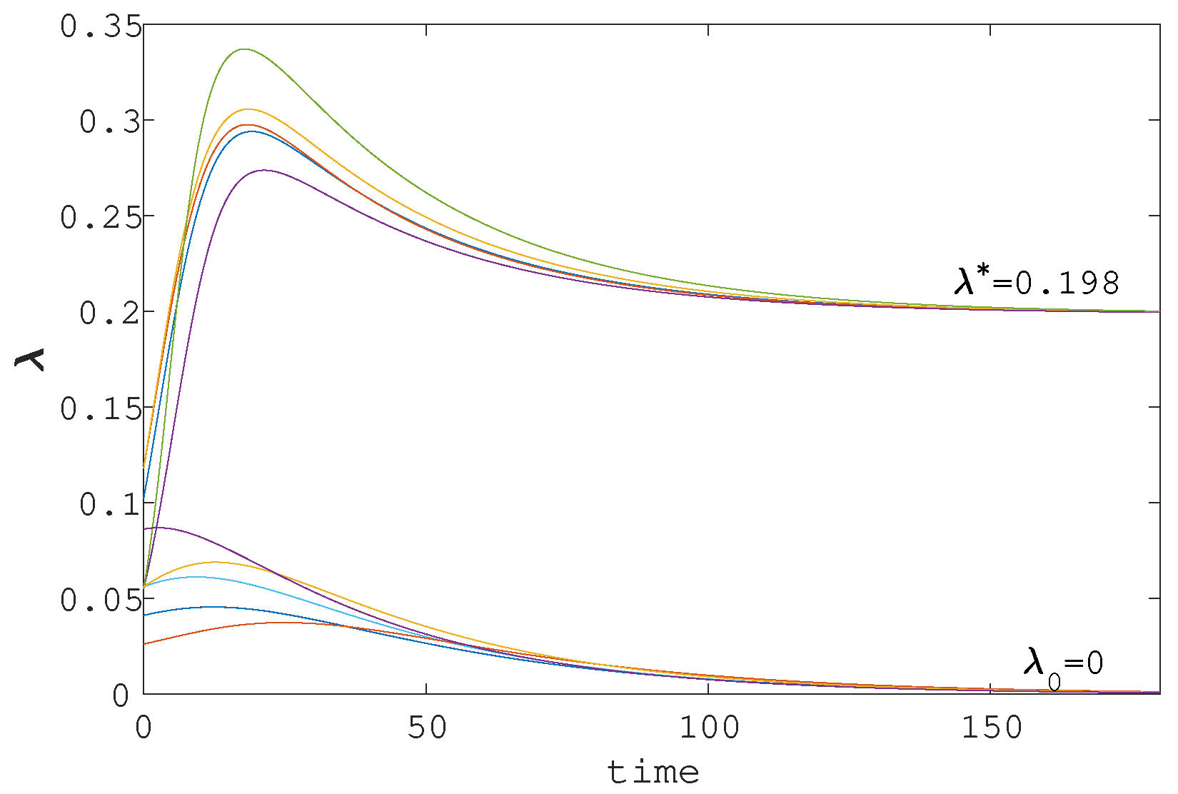
In Figure 2, different values for the threshold number are chosen to explain the stability of system (6). It can be noticed how $\lambda$, which is the percentage of infected nodes as a function of time t, converge to ${\lambda }^{\ast }$ or ${\lambda }_0$ depending on the value of ${\mathcal{R}}_0$. In words, if ${\mathcal{R}}_0>1$, then the values of $\lambda$ converge to ${\lambda }^{\ast }$ with time t, and if ${\mathcal{R}}_0<1$ then the values of $\lambda$ converge to ${\lambda }_0$ with time t. The values of the used parameters are as follows:

$$(\beta ,ϵ,\eta ,{\gamma }_l,{\gamma }_h,{\xi }_l,\xi ,{\xi }_h,\mu )=(0.315,1,1,0.029,0.052,0.85,0.103,0.302,0.013)$$

with $R_{0a}=2.7099$, and we set

$$(\beta ,ϵ,\eta ,{\gamma }_l,{\gamma }_h,{\xi }_l,\xi ,{\xi }_h,\mu )=(0.15,1,1,0.0292,0.283,0.38,0.1031,0.302,0.081)$$

then $R_{0a}=0.8134$.

In the next section, different examples and experiments are proposed to solve system (6) and to show the stability.

4. Numerical Analysis and Discussion

In this section, different examples and experiments are proposed to solve system (6). Furthermore, numerical techniques are used to approximate the solution. These examples illustrate the stability as well, and reversing symmetry transformation is shown.

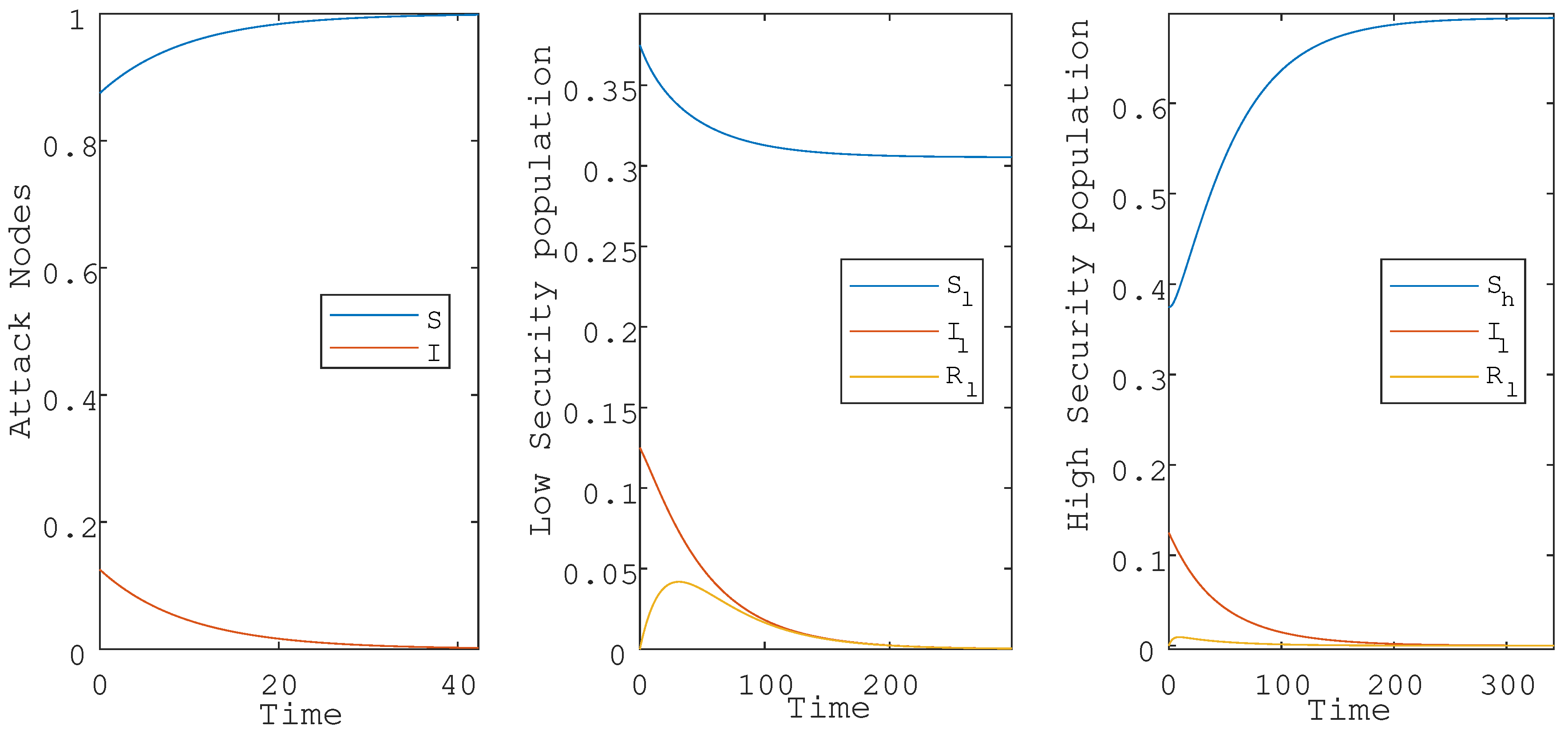
Example 1.

Solve system (6), in which the values of the parameters are the following: $(\beta ,ϵ,\eta ,{\gamma }_l,{\gamma }_h,{\xi }_l,\xi ,{\xi }_h,\mu )=(0.015,0.61,1,0.029,0.028,0.05,0.103,0.302,0.013)$ with initial conditions $(S\left(0\right),I\left(0\right),S_l\left(0\right),$$I_l\left(0\right),R_l\left(0\right),S_h\left(0\right),I_h\left(0\right),R_h\left(0\right))=(0.875,0.125,0.375,0.125,$$0,0.375,0.125,0)$, $R_{0a}=0.129$, and $R_{0t}=0.7204$.

Since $R_{0a},R_{0t}<0$ then ${\mathcal{R}}_0<1$. Therefore, it can be concluded that the system will be infection-free with time. Hence, the trajectories of the solution converge to $P_0=(1,0,0.3,0,0,0.7,0,0)$, as shown in Figure 3. Moreover, we notice that the attack node population is invariant with respect to the reversing symmetry transformation described in Lemma 1 for a small value of $\mu$.

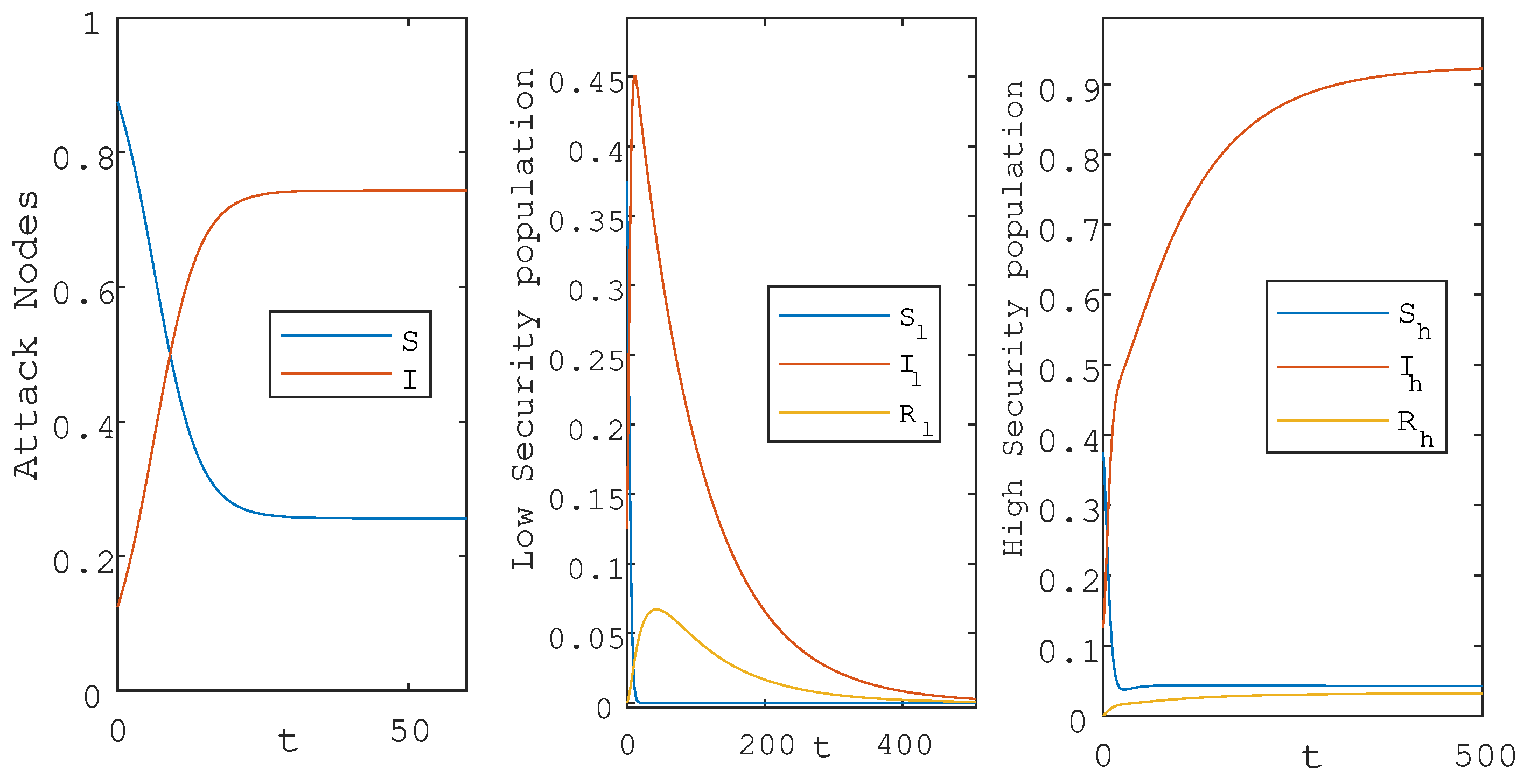
Example 2.

Solve system (6), in which the values of the parameters are chosen as: $(\beta ,ϵ,\eta ,{\gamma }_l,{\gamma }_h,{\xi }_l,\xi ,$${\xi }_h,\mu )=(0.34,0.61,1,0.0102,0.0102,0.051,0.068,0.302,0.0201)$ with initial conditions $\left(S\right(0),$$I\left(0\right),S_l\left(0\right),I_l\left(0\right),R_l\left(0\right),S_h\left(0\right),I_h\left(0\right),R_h\left(0\right))=(0.875,0.125,0.375,$$0.125,0,0.375,0.125,0)$, $R_{0a}=3.9$, and $R_{0t}=46.7117$.

It can be concluded that the system is epidemic since ${\mathcal{R}}_0>1$. Since $R_{0a},R_{0t}>1$, then ${\mathcal{R}}_0>1$. Therefore, the system will be infected, and the trajectories of the solution converge to $P_{\ast }$, as illustrated in Figure 4.

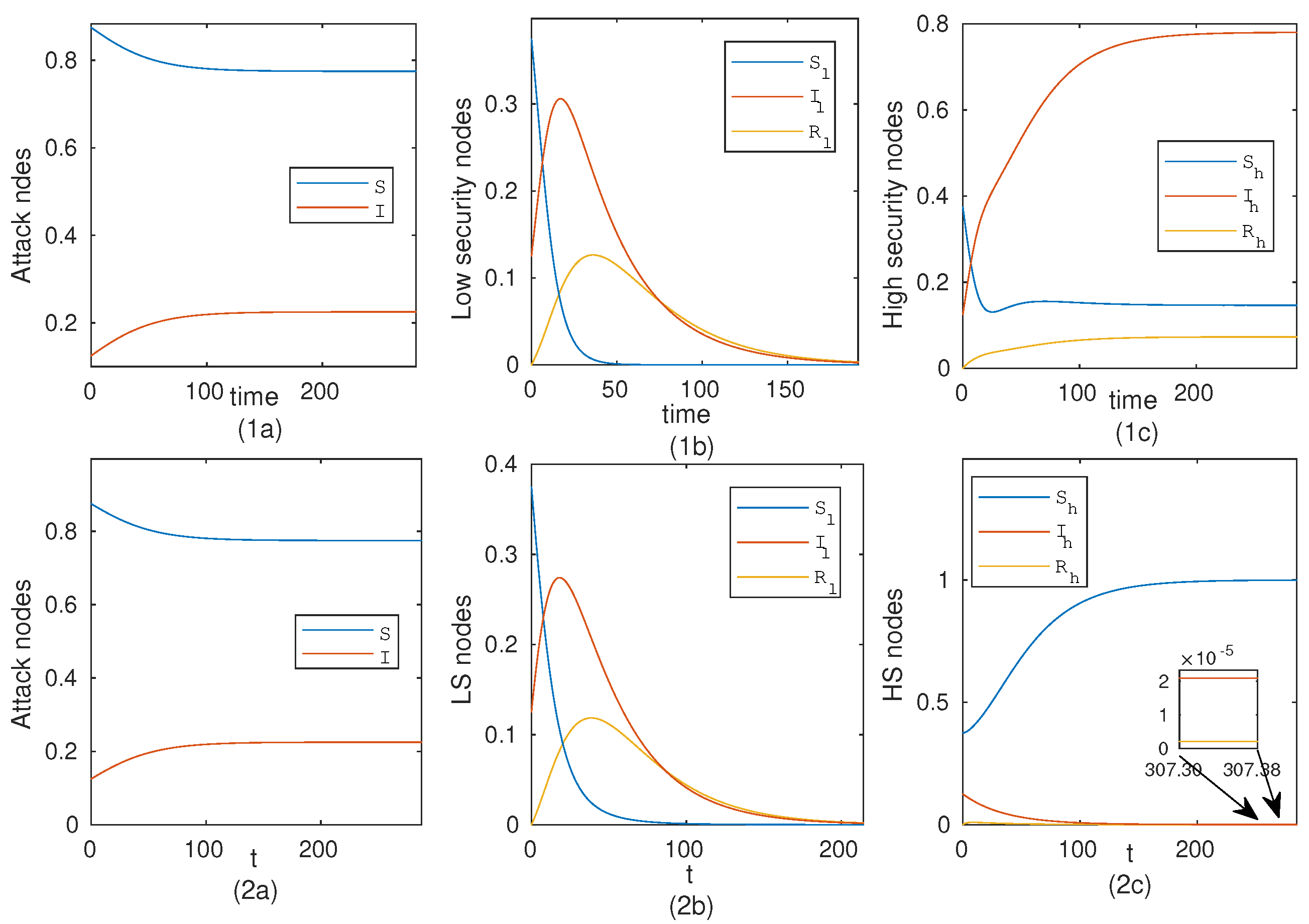
Example 3.

In this example, the solution of system (6) solved with perfect high and low-security levels. $(\beta ,\eta ,{\gamma }_l,{\gamma }_h,{\xi }_l,\xi ,{\xi }_h,\mu )=(0.15,1,0.0292,0.0283,0.051,0.1031,0.302,0.01314)$ with initial conditions $(S\left(0\right),I\left(0\right),S_l\left(0\right),I_l\left(0\right),R_l\left(0\right),S_h\left(0\right),I_h\left(0\right),R_h\left(0\right))=(0.875,0.125,0.375,$$0.125,0,0.375,0.125,0)$.

Example 3 shows the efficiency of $ϵ$ when we have a perfect high-security level. In Figure 5, class 1 ((1a), (1b), and (1c)) represent the solution when $ϵ=0$, and class 2 ((2a), (2b), and (2c)) represent the solution when $ϵ=1$. By comparing these two classes, it can be concluded that figures (1a) and (1b) and figures (2a) and (2b) are the same, but the difference between the two experiments is at the last stage when $ϵ=1$ (high-security), in which the system is converted from epidemic to almost infection-free. Additionally, the attack node is invariant with respect to the reversing symmetry map for small death rate.

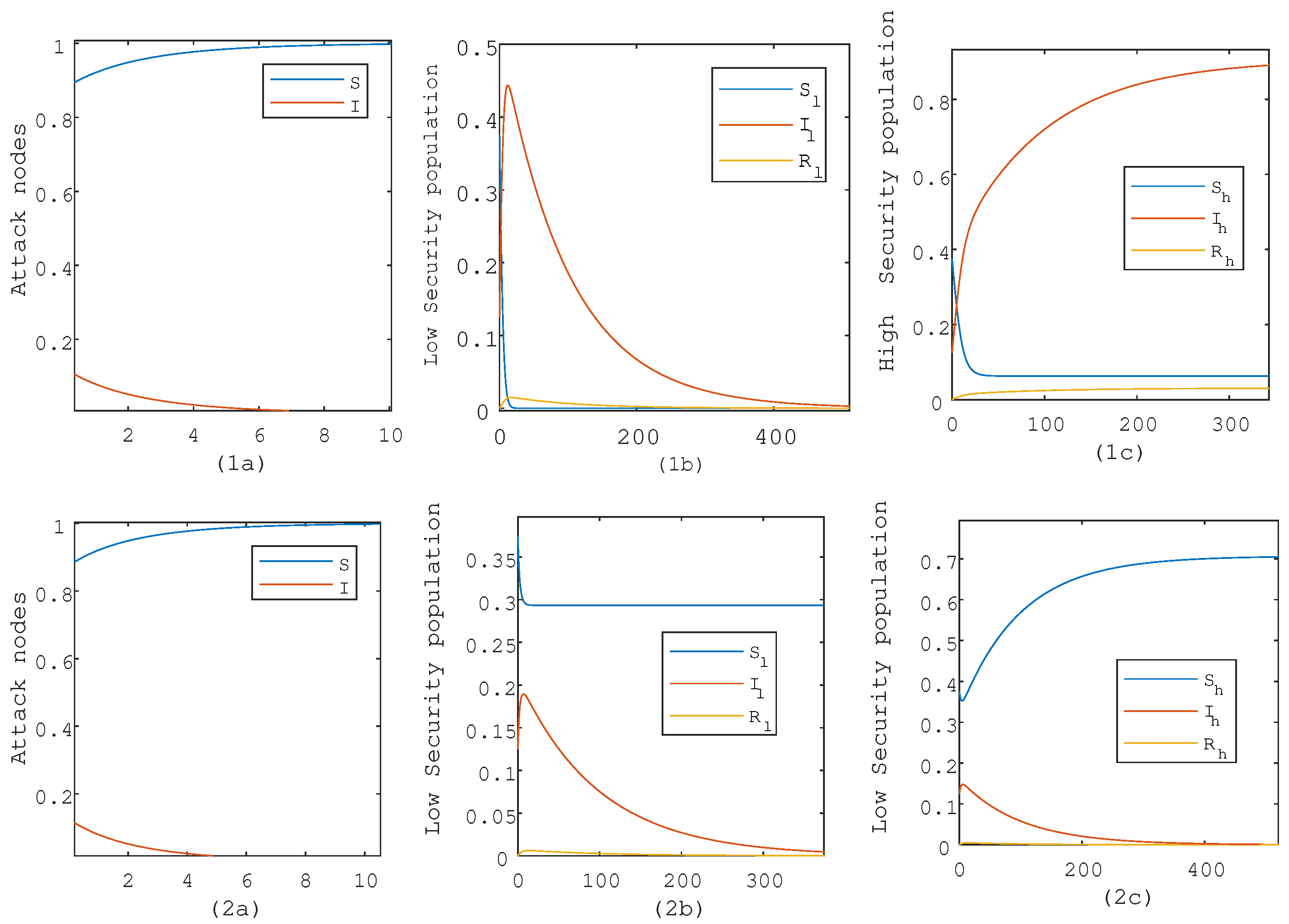
Example 4.

Solve system (6) for different values of η ($\eta =0,\eta =0.5$), with parameters $(\beta ,ϵ,{\gamma }_l,{\gamma }_h,$${\xi }_l,\xi ,{\xi }_h,\mu )=(0.831,00.61,0.0102,0.0102,0.3,0.6851,0.3,0.5201)$ with initial conditions $(S\left(0\right),I\left(0\right),S_l\left(0\right),I_l\left(0\right),R_l\left(0\right),S_h\left(0\right),I_h\left(0\right),R_h\left(0\right))=(0.875,0.125,0.375,0.125,$$0,0.375,0.125,0)$.

In Figure 6, the first class ((1a), (1b), and (1c)) represents the solution of system (6) when $\eta =0.5$, i.e., when the attacker exploited the infected target devices to attack other nodes. This effect is represented by $\eta$. Figures (2a), (2b), and (2c) in the second class represent the system when $\eta =0$, i.e., when the attacker could not use the target infected devices to increase the effect of the attack. Therefore, it can be noticed that in the first class, the attack remains in the system since $R_{0t}>1$ despite $R_{0a}<1$. However, in the second class, the attack disappears because of $\eta =0$. The result of Lemma 1 can also be noticed in the attack node population (1a) and (2a).

5. Conclusions

In this paper, we proposed a mathematical model to describe DDoS attacks. One of the most significant features of this model is considering a high-security level for the target population in which the recovered nodes upgrade their defense level to a higher level. In previous models, the recovered nodes did not have any upgrade on their defense level, which is an unrealistic assumption. Therefore, we set $ϵ$ to represent the firewall efficiency after recovering. Furthermore, the modification parameter $\eta$ was set to account for the attack transmission of the infected target nodes (in the $I_l$ and $I_h$ compartments). Moreover, we analyzed the proposed model for certain cases. The threshold value (${\mathcal{R}}_0$) was found, and the stability was discussed. The reversing symmetry transformation $\mathcal{T}$ of the attack population was described. Finally, different examples were presented to illustrate the validity of the proposed model (6).