Article

Three-Phase Feeder Load Balancing Based Optimized Neural Network Using Smart Meters

1
Electrical Power Engineering, Yarmouk University, Irbid 21163, Jordan
2
National Electric Power Company, Substation Maintenance Department, Amman 11181, Jordan
3
Irbid District Electricity Company, Planning Department, Loads Management Section, Irbid 21100, Jordan
*
Author to whom correspondence should be addressed.
Symmetry 2021, 13(11), 2195; https://doi.org/10.3390/sym13112195
Submission received: 11 October 2021 / Revised: 2 November 2021 / Accepted: 12 November 2021 / Published: 17 November 2021
(This article belongs to the Topic Dynamical Systems: Theory and Applications)

Abstract

:
The electricity distribution system is the coupling point between the utility and the end-user. Typically, these systems have unbalanced feeders due to the variety of customers’ behaviors. Some significant problems occur; the unbalanced loads increase the operational cost and system investment. In radial distribution systems, swapping loads between the three phases is the most effective method for phase balancing. It is performed manually and subjected to load flow equations, capacity, and voltage constraints. Recently, due to smart grids and automated networks, dynamic phase balancing received more attention, thus swapping the loads between the three phases automatically when unbalance exceeds permissible limits by using a remote-controlled phase switch selector/controller. Automatic feeder reconfiguration and phase balancing eliminates the service interruption, enhances energy restoration, and minimize losses. In this paper, a case study from the Irbid district electricity company (IDECO) is presented. Optimal reconfiguration of phase balancing using three techniques: feed-forward back-propagation neural network (FFBPNN), radial basis function neural network (RBFNN), and a hybrid are proposed to control the switching sequence for each connected load. The comparison shows that the hybrid technique yields the best performance. This work is simulated using MATLAB and C programming language.

1. Introduction

The electricity distribution systems are typically unbalanced because of the continuous change in customer loading profile during the day. Once the three phases are not adequately balanced, the risk of over-loading in the network equipment and the power losses increase. Subsequently, the system stability is affected, the supply quality is decreased, and the electricity cost is increased [1]. On the other hand, load balancing improves the reliability and security of the electrical network. Load balancing also minimizes system losses to relieve transformer loading [2,
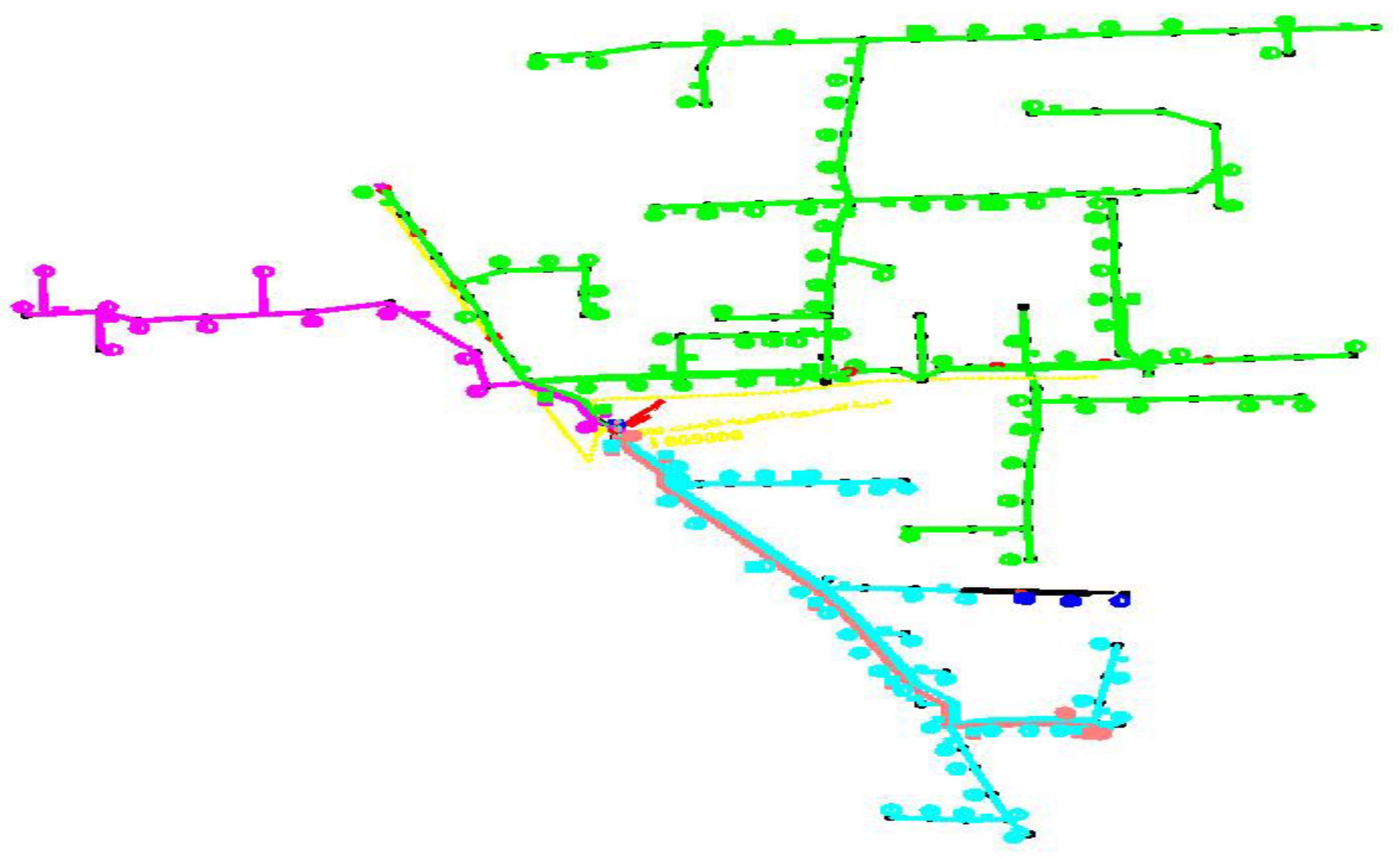
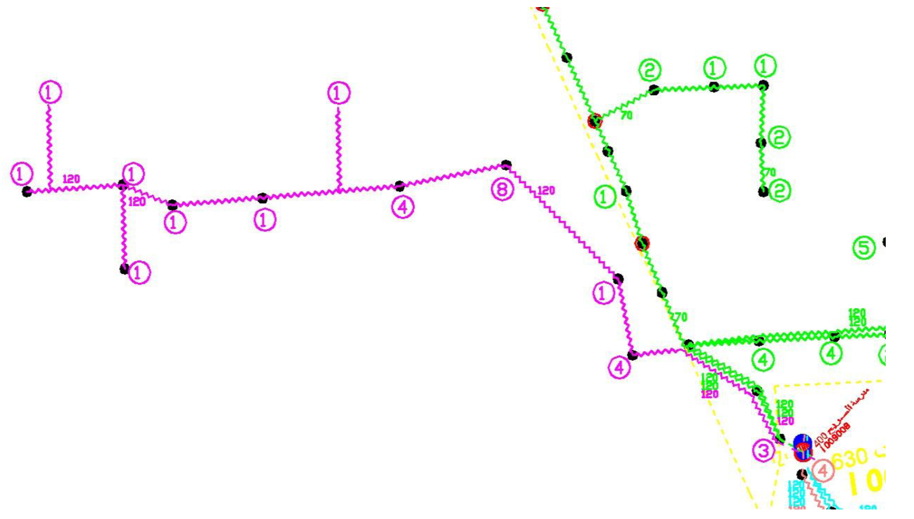
3]. Imbalanced three-phase feeders can be reconfigured by implementing some load balancing techniques such as phase swapping and feeder reconfiguration. The phase swapping technique changes the distribution of loads by swapping them between the phases to make the three phases as equal as possible without changing the feeder topology, as shown in Figure 1 and Figure 2, respectively. Data obtained from the smart meters which are installed at the beginning of each low voltage feeder and customer side are sent directly to the remote controller (brain) to calculate the losses on the feeder. Feeder losses are computed as a difference between the feeder and the summation of the customers’ consumption. After that, the controller gives orders to a one-way switching device to take action—if needed—to swipe between the phases feeding customers. Data sent to the controller can be classified into fixed data and variable data, as shown in Figure 3. Fixed data can be introduced as the data regarding the network topology, such as cable lengths, sizes, and configuration, and customer data such as customer numbers at each connection node. While the variable data are the data that come from the main smart meter fixed at the beginning of the low voltage feeder containing power and energy, and the data coming from the smart meters fixed at the customer side, containing the power and energy consumption, as well.
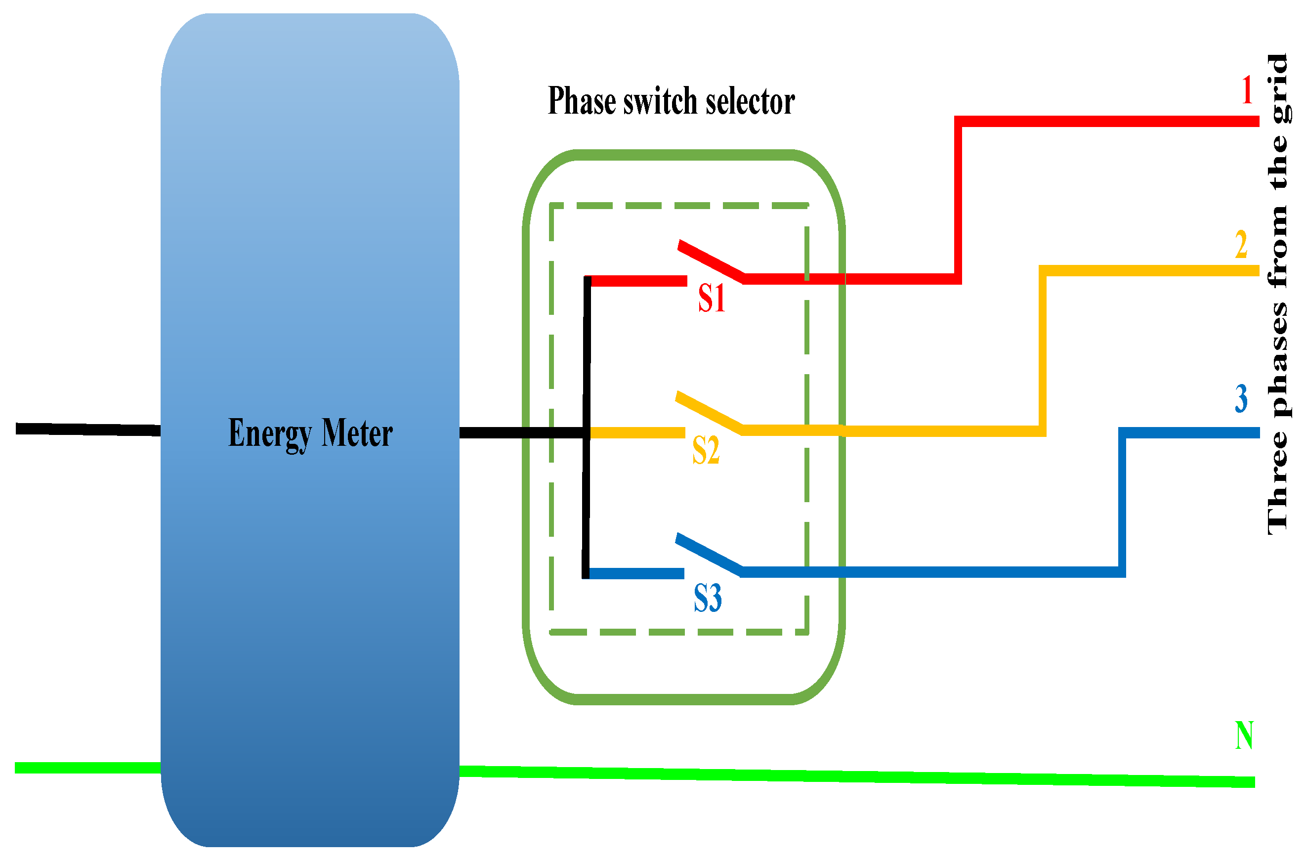
This mechanism is implemented using a phase switch selector/controller installed right before the energy meter at the customer side and swapping the customers between the three phases on the same feeder to maintain continual phase balancing. When three phases are connected to the phase switch selector’s input side, only one switch should be closed as an output, while the other two phases should remain open, as shown in Figure 4.
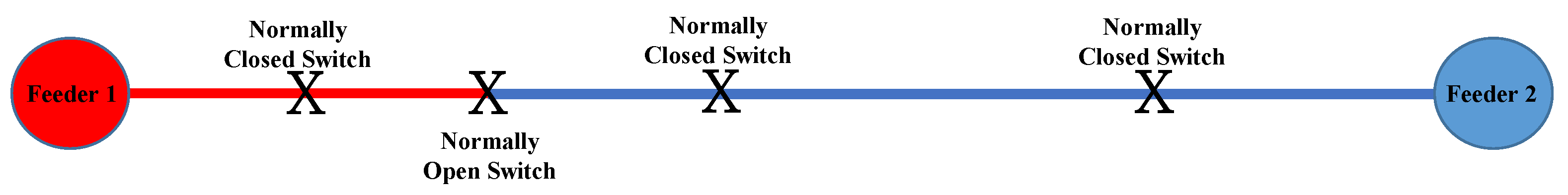
The feeder reconfiguration technique changes the feeder topology by moving parts of the feeder to an adjacent one by changing the switches’ status so that loads are switched from one feeder to another to relieve the loading of an overloaded feeder to a lightly loaded one [4,5]. Usually, feeder reconfiguration shifts the loads from the heavily loaded feeder to another lightly loaded feeder. Practically, electricity distribution utilities perform load balancing with manual trial and error technique, which is time-consuming, costly, and does not guarantee phase loading equality. Phase balancing automation becomes more realistic, resilient, and agile. It is implemented through power electronics, modern communication techniques, and artificial intelligence. Different types of neural network-based approaches are presented in this work to control the switch selector output to swap customers between the phases. Along with the low voltage distribution feeders, several customarily opened and normally closed switches are distributed to allow transferring load currents between the feeders [6].
Distribution systems operate under constraints to assure the continuity of supply to the customers under certain quality. The distribution feeders consist of a variety of loads under different categories. This variation in load types and their peak demands do not coincide. Therefore, a variation in loading on some parts of the feeder during the day is noticed. Hence, it is essential to reconfigure the network by rescheduling the loads to operate the system effectively [7]. Feeder reconfiguration modifies the topology of the distribution system by changing the open and close status of switches to better the distribution networks, whereas phase swapping changes the customer connection from one phase to another. The load balancing analysis determines which loads can be reconnected to different phases. Load balancing in the distribution system is defined as preserving the load currents roughly identical to the three phases. Loads are considered evenly distributed on the three phases; i.e., each phase should be connected to 1 / 3 of the total loads. So, the problem is to find the most appropriate three sets of loads, with minimum differences among the individual sums of the three sets.
The loss minimization in distribution system reconfiguration and load balancing problems of the open-loop radial power are presented using different techniques such as heuristic or meta-heuristic approaches [8,9,10], mathematical programming [11], and intelligent algorithms [12,13]. The heuristics techniques produce acceptable results with less computation cost. The network reconfiguration with optimal distribution generators siting, sizing, and tie-switch placement for reliability improvement and loss minimization is proposed [14]. The loss minimization using reconfiguration and switching modifications like closing or opening the sectionalizing switches of the distribution feeders are manipulated. A three-phase load balancing using load flow variation technique before electrical installation is presented [15,16]. Load balancing estimation using balancing index calculation is formulated as a non-linear optimization problem with an objective function [17]. Reducing the feeder unbalance using a fuzzy logic is demonstrated [18,19]. Different techniques are carried out to maintain the load balance, such as Ant Colony Optimization [20], support vector machines [21,22], and discrete passive compensator [
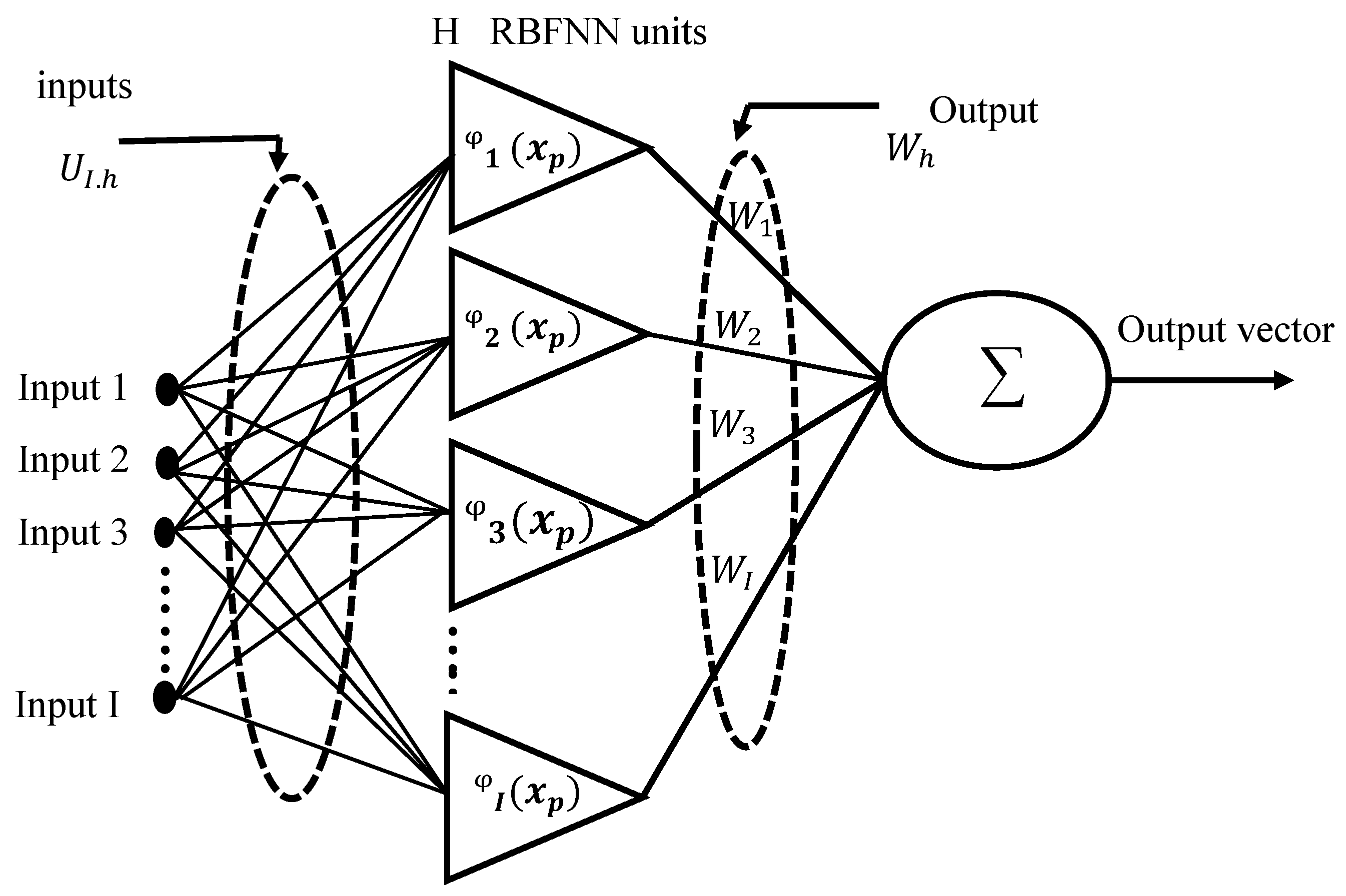
23]. This work is a real case study for an optimal automatic feeder reconfiguration using three-phase load balancing based artificial neural network (ANN) techniques: radial basis function neural network (RBFNN) [
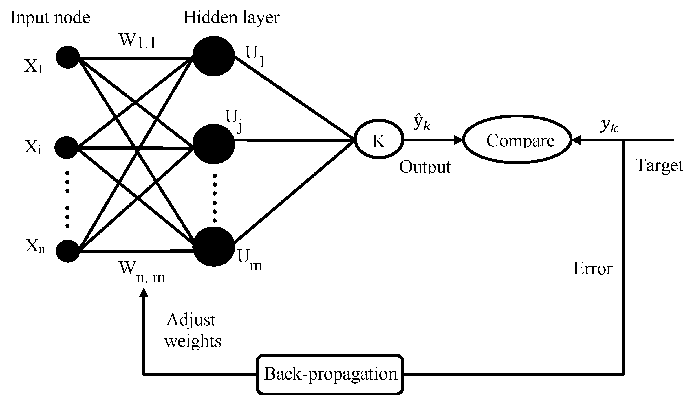
24], feed-forward back-propagation neural network (FFBPNN) [25], and a hybrid. Implementing a hybrid technique is the original contribution. This technique enhances the learning process of FFBPNN, rides over the local minima, speeds the slow rate error convergence, and reforms classification precision.
The rest of this article is organized as follows. Section 2 discusses load balancing. Next, the system techniques under study is presented. ANN techniques are discussed, including RBFNN, FFBPNN, and hybrid techniques are addressed in Section 4. Results and discussion are discussed in Section 5, followed by a conclusion in Section 6.

2. Load Balancing

Distribution network operators face continuous pressure to improve the quality of supply for customers and decrease operating losses. Unbalanced loading of distribution feeders is one of the essential factors affecting low voltage networks’ overall losses. The asymmetry factor is high when the overall loading is low, and the asymmetry is significantly smaller during peak load. It means the system is extensively trying to symmetrize the load during the periods with low loading and minimal effect on the overall losses. Thus, the unbalanced loading of the three-phase feeder’s distribution and the impact of unbalance currents on the overall losses are considered a hot topic. Electrical utilities modernize power generation and distribution systems. The electric grid transformation offers improved performance and growth opportunities for customers, communities, and businesses. The system deployed in this study is considered the first step towards advanced metering infrastructure that integrates smart meters, software, data centers, and communication networks. Electric companies can enhance their customer services and operations.
The problem is about determining the switches that be opened or closed to obtain load balancing among feeders. Many constraints should be kept, such as voltage drop, thermal constraint, reliability constraint, and capacity constraint of distribution lines and transformers to achieve equal phase loading. The load is dynamic during the day due to the customer’s behavior and usage of their appliances. Hence some phases are lightly loaded during a certain period of the day and heavily loaded at another time.
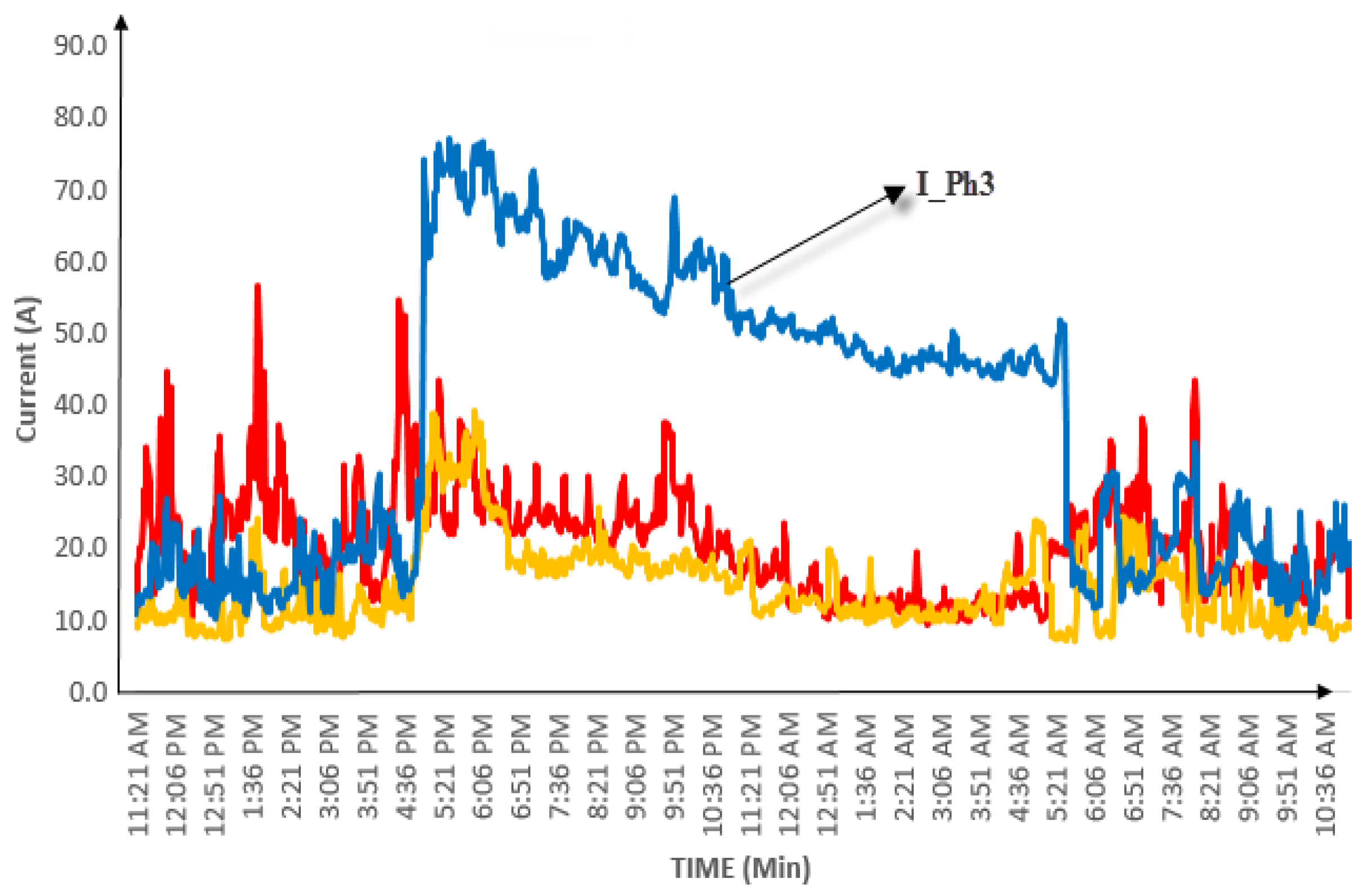
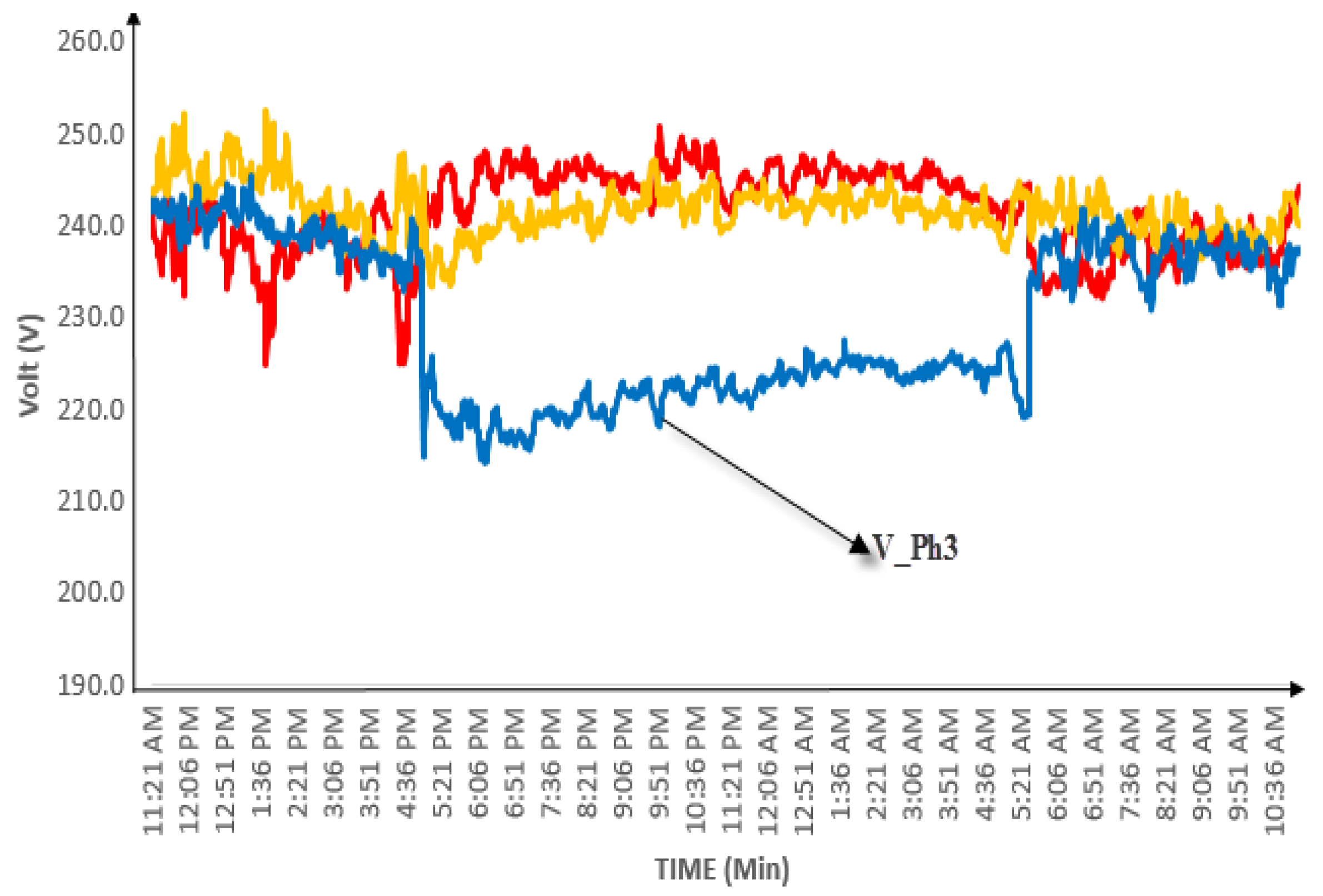
 Figure 5 and Figure 6 show an example for the unbalanced three-phase loads currents and voltages, respectively. This load is a pure residential load located in Ajlun district. Customers are swapped between the phases continuously to achieve load balancing on the feeder and the transformer. When the smart meters’ data are sent to a remote server, it starts to check through optimization techniques if there is any better arrangement for the customers on the three phases to obtain load balancing. If yes, orders are sent to the phase switch selector to swap the customer between phases, with a super-fast action to avoid supply discontinuity. Otherwise, the current situation is the best customer arrangement, and it does nothing [26].
The phase switch selector takes an order from a remote server that collects data from the downstream smart energy meters, calculates the losses at the current situation, and rearranges the loads using one of the proposed algorithms to guarantee the best phase balancing and minimum losses. The new configuration is sent to the phase switch selector to be implemented. Thus, the phase switch selector takes a three-phase input from the grid; each phase is connected to a switch. One switch of those three switches is closed, while the other should remain open. When an order comes from the server to swap the connected customer from phase A to phase B, a super-fast switching is made to open the switch connected to phase A and close the switch connected to phase B. Discontinuity of supply would not affect the customers because it should be super-fast switching according to the phase switch selector characteristics. This fast-switching time should be mentioned in the datasheet of the phase switch selector and should be fast enough that the customers’ appliances would not affect it [27].

3. System under Study

In Jordan, distribution feeders are a three-phase, four-wire system. Usually, they are radial or open-loop structures with the same conductor size along the feeder. Balancing loads on a three-phase feeder and reducing neutral current, improving voltage profiles, reducing losses and enhancing system stability and reliability is a very sophisticated task for the utility and engineers because they do not have authority or monitoring over their customers. Practically, phase balancing is carried out manually by trial and error technique based on experience and engineer’s knowledge about customer’s behavior in that area. By using this manual trial and error method, supply interruption is inevitable when exchanging customers’ connection phases to another.
A real case study from IDECO (latitude: 32°33 20.02 N, longitude: 35°51 0.00 E) is considered in this work. One of four radial feeders going out from a 630 KVA transformer in the Irbid district is chosen. The feeder under this study has 27 customers, is 470 m in length, and has a 120 mm 2 cross-sectional area. Smart meters are installed along the feeder at the customer side. Their consumption varies from 0.2 kW to 5 kW. Figure 7 shows a schematic diagram for the transformer and the corresponding low voltage network of the four feeders coming out of it, including the feeder under study, while Figure 8 shows a schematic diagram for the same feeder understudy and the number of customers connected to each node. The number of customers equally on the three-phase is not necessary for load balancing, but the current equality on the three phases. In some countries, almost all residential customers have a three-phase connection, but this method is used for single-phase.

4. ANN Techniques

RBFNN

RBFNN is an ANN technique that was formulated in 1988 by Broomhead and Lowe. It depends on the linear activation function stored in both input and output layers, whereas the Gaussian activation radial basis function is stored in the hidden layer as shown in Figure 9. However, there are three main parameters; a center that can be determined using clustering techniques, the transfer function, and the distance measured between the input layer and the center. The number of neurons in both input and output layers is determined based on the training pattern, whereas the number of neurons in the hidden layer is determined based on the system’s non-linearity. The mathematical model of RBFNN can be represented as follows [28].
f ( I ) = Ψ I c i r i 2 2
where I is the input vectors, f(I), r i , and c i are the output, radius, and center of ith neurons in the hidden layer, respectively. Ψ is the radial basis function, q is the number of input in the training process and I c i is the distance between the input vectors and the center c i in the Euclidean space. Clustering technique is used to calculate the center location and is given by Equation (2) [29].
I c i = ( I 1 c i 1 ) 2 + ( I 2 c i 2 ) 2 + + ( I q c i n i ) 2
The width G t r of the basis function ( σ ) and the weight of the output layer W is given by Equations (3) and (4), respectively [29].
G t r I q c i 2 = e N h d m a x I q c i 2
W = G t r + × Y t r
The output Y of RBFNN can be obtained using Equation (5) [29].
Y = W T × G t s t T
where G t s t is given in Equation (6) and the suffix t s t is for testing input vector obtained for certain desired output. Figure 10 shows the main procedure to train RBFNN. It is started with collecting the required data, then selecting the appropriate input and optimum values of the number of neurons in the three layers with their appropriate weight and determining the suitable activation function. Finally, training the network and calculating the error [29].
G t s t I t s t c i 2 = e I t s t c i 2 2 σ 2

FFBPNN

Here, the main goal is to minimize the whole network’s error by reducing each output neuron’s error. The ANN should detect how to map arbitrary input to the output suitably by optimizing the weights. This technique has many features, including accuracy, decreasing the training time, enhancing the processing speed, optimizing the cost function, and improving the mean absolute percentage error (MAP) [31]. The back-propagation algorithm can be described in the FFBPNN technique as shown in Figure 11; the network is created, then the network is trained by giving the input to innovate the output. Thus the network is learned to examine all the values throughout the network. Here, the forward propagation technique can be applied, which means that the input innovates the output, then the backward propagation, including the error being estimated backward towards the input. Lastly, the weight is adjusted, and the error can be reduced by adjusting the weight function. The name of the back-propagation comes from the process sequence [32]. It starts from the input towards the output, then propagates back from the output to the input as shown in Figure 12. Moreover, adjusting the activation functions and the bias through going across. For the first time, these outputs make no sense, but better results are obtained by decreasing error after repeating the process more and more. This algorithm as shown in Figure 13 starts with having new observation x = [ x 1 x d ] and target y * , then feed forward for each unit g i in each layer 1 L and compute g i based on units f k from previous layer as shown in Equation (7)
g i = σ u j o + u j k f k
After that, get the prediction y and the target y 2 and calculate the error ( y y * ) . For each unit g i in each layer L 1 , an error can be calculated on both g i and on u j k that affects g i using Equations (8) and (9), here a sort of synthetic training model is created for all the hidden units in the network, and the errors are propagated by computing the derivative of the error with respect a unit g in the network. The interpretation of the derivative determines to higher or lower of the unit g. Subsequently the g units affects the h units and updating the weight v i j . The nodes are sigmoids and the scaling function σ ( h i ) states that H was around zero or one, then whatever changes made to G are not affected. H determines whether G is high or low. Further, the weights f k that connect G to the nods are higher or lower, as shown in Equation (9). The derivative indicates that the strength is higher or lower. In this logistic process, each iteration, this strength is updated as well as the weight as shown in Equation (10) [33].
E g i = i σ ( h i ) v i j E h i
E u j k = E g i σ g j f k
u j k u j k η E u j k
The difference between the output y and the target y * is calculated using Equation (11). The derivative of the error concerning the unit h i in the last hidden layers is as shown in Equation (12). The value of derivatives of the error concerning the hidden layers is computed as sigmoid y ( 1 y ) of the bias is added to the weighted product of both the combination of the previously hidden layer and strong connection of the two layers as shown in Equation (13). The derivative of error concerning g is as the same as before. It is shown in Equations (14)–(16), respectively. This nest can be handled as many layers deep as suggested. Clearly, Equations (9)–(16) are the proof for Equation (8) as well as optimizing the error with respect to all of the parameters [34].
E = 1 2 y y * 2
E h i = y y * y ( 1 y ) w i
E g i = y y * y g i
E g i = y y * y ( 1 y ) i w i h i g i
E g i = y y * y ( 1 y ) i w i h i ( 1 h i ) v i j
E g i = i h i ( 1 h i ) v i j E h i

5. Results and Discussion

The performance of the proposed model is evaluated, different evaluation measures have been adopted, including mean absolute percentage error (MAPE), mean squared errors (MSE), and the root means squared error (RMSE).
  • MAPE: It shows the deviation of the predicted errors that show how much the predicted points are close to the target line, represented by Equation (17).
    M A P E = 1 n i = 1 n ( y i y ^ i ) 2
  • MSE: It is the average of the magnitude of the predicted errors, presented by Equation (18).
    M S E = 1 n i = 1 n | y i y ^ i |
  • RMSE: It shows the deviation of the predicted errors that show how much the predicted points are close to the target line, represented by Equation (19).
    R M S E = i = 1 n ( y i y ^ i ) 2 n
    where n is the number of observations, i = 1 , 2 , 3 , , n . y i is the measured value, and y ^ i is the forecasted value. The simulation is executed on an Intel Core i7-8750H CPU, 2.20 GHz, 64.0 GB RAM computer. The proposed ANN is implemented using Mathworks/MATLAB. Different ANN techniques are used, selecting the appropriate number of hidden layers and the number of neurons is the most critical step. This step leads to quick training speed, reduced memory space, and acceptable global generalization capability. The main drawback of an inappropriate number of hidden nodes may be over-fitting for the input data. The ANN technique is used to solve the load balancing problem. There are around 10,000 samples used as real data obtained from IDECO. Each sample holds current measurements for 27 different loads (houses). It is used to control the switching sequence of each load to keep the three phases balanced. The recorded data are distributed as follows: training set 75 % , validation set 10 % , and testing set 15 % . The ANN inputs are the unbalanced 27 load currents, and the outputs are the switch sequences for each load. The network’s output is in the range of (1, 2, 3) for each load. It means the phase number on which switch should be closed or opened for that specific load. The balanced output loads are obtained from implementing a heuristic technique, and they are used to train, test, and validate the ANN. A Matlab/Mathworks command (newff) is used to implement FFBPNN for the whole feeder with an input and output matrices are (10,000 × 27 ) and ( 3 × 10,000), respectively. 
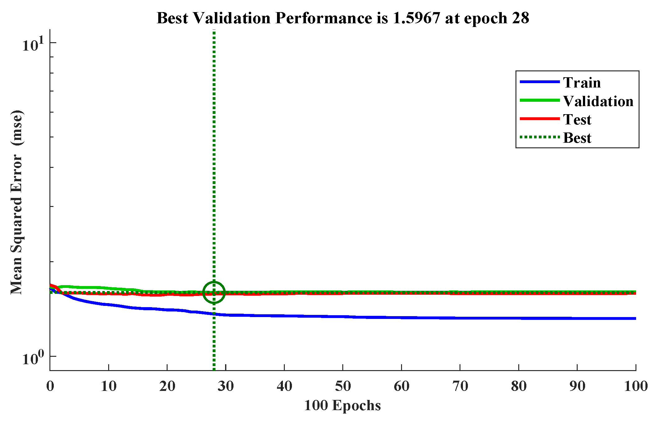
Figure 14 shows the best validation performance for FFBPNN.
Table 1, Table 2 and Table 3 evaluate MAPE, MSE, and RMSE errors, respectively for 10,000 current samples for I p h 1 , I p h 2 , and I p h 3 using FFBPNN for different layer architecture and different iterations (10,100,1000). For example, the first row (10-10-10) means that there are three hidden layers. Each hidden layer contains ten neurons. The optimal performance belongs to the configuration 2000, which means one hidden layer with 2000 neurons. Error evaluations for this technique failed in the load balance test, and therefore it is not recommended in such cases. The distribution of the currents on the three phases was far from the actual currents, and the rate errors were not acceptable. Table 4, Table 5 and Table 6 evaluate the average error current in terms of spread constant and the number of neurons for 10,000 samples on I p h 1 , I p h 2 , and I p h 3 , respectively using RBFNN. The configuration (5:1000) has optimum evaluation in terms of MAPE, MSE, and RMSE. The errors were 0.15 % , 3274, and 57.22 % for phase 1, 0.24 % , 3560, and 59.67 % for phase 2, and 0.15 % , 3274, and 57.22 % for phase 3, respectively. Table 7, Table 8 and Table 9 evaluate errors for the three phases using the hybrid technique. This technique has much better results than the two individual techniques in terms of performance and errors calculations.
The configuration (5:1000) has optimum evaluation in terms of MAPE, MSE, and RMSE errors. The results were 0.06 % , 664, and 25.75 % for phase 1, 0.06 % , 663.67 , and 25.67 % for phase 2, and 0.06 % , 678.33 , and 26.04 % for phase 3, respectively. It is highly recommended for three phases of electrical load balance.
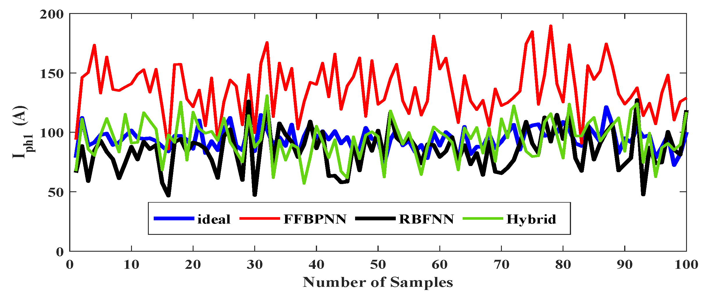
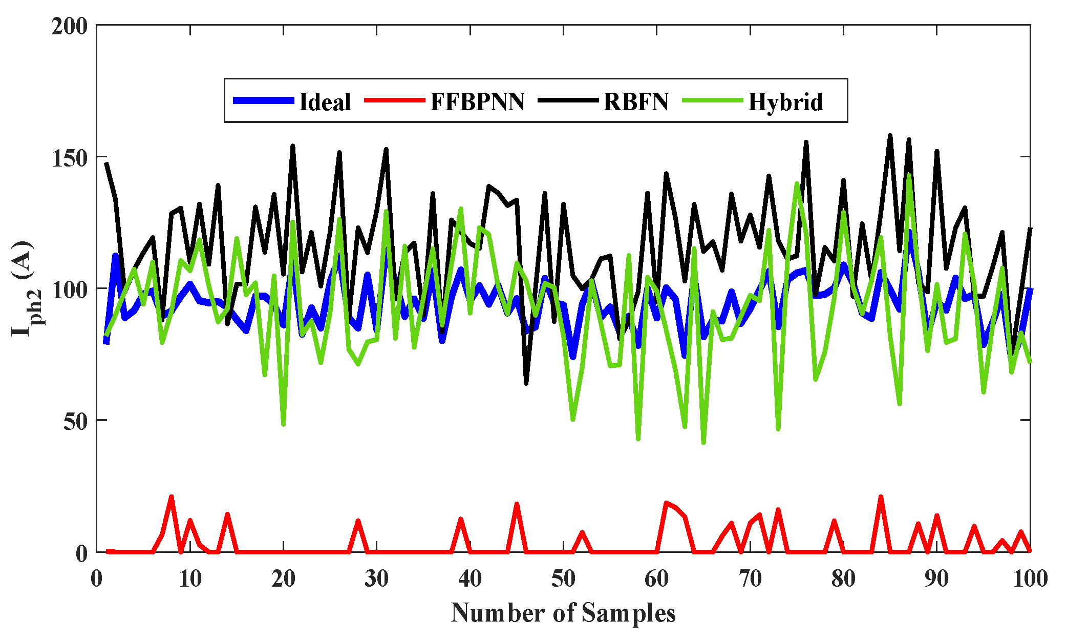
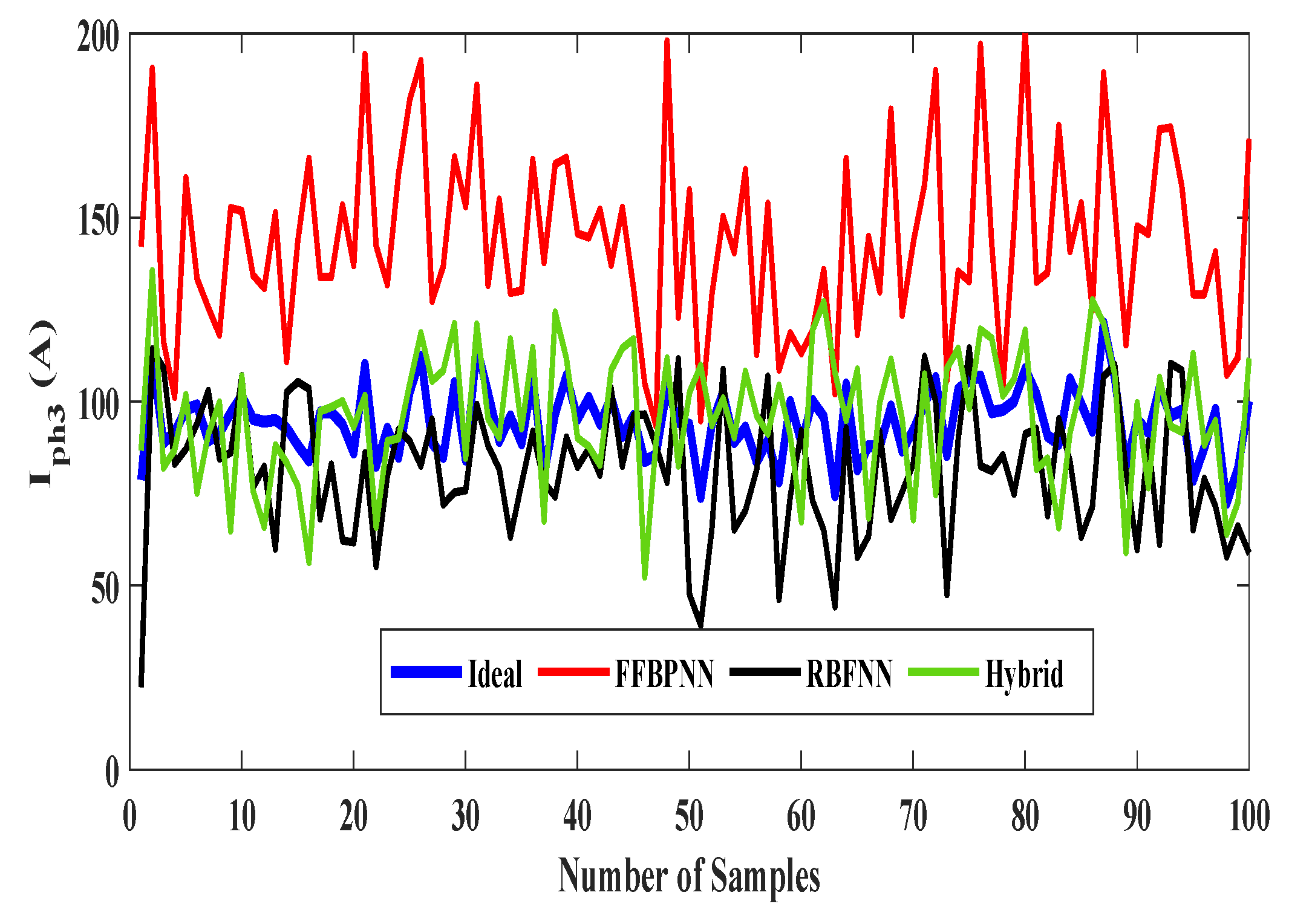
 Figure 15, Figure 16 and Figure 17 show the three phases currents via I i d e a l for the three techniques. Hence, the hybrid technique has the best performance in phase balancing studies. It is practical, flexible, and recommended to IDECO.

6. Conclusions

This work presents a MATLAB-based solution for ANN techniques for load balancing investigation. These techniques are successfully tested and validated using simulated real data. The testing results obtained show that the FFBPNN technique has a significant deviation from the desired ideal current. The results obtained using this technique are the worst. On the other hand, the hybrid technique is more guaranteed to give analytical results for load balancing problems than using FFBPNN or RBFNN techniques individually. It showed a better convergence, faster training, and classification thoroughness using a discrete data set; moreover, the results were very close to the ideal values of currents and the acceptable error profiles. This technique is considered the most operative, and it is highly recommended that IDECO use it in load balancing studies since the three-phase balancing has many advantages for customers and utilities.

Author Contributions

Conceptualization, L.A., Q.N. and W.M.; methodology, L.A., Q.N. and W.M.; software, Q.N.; validation, L.A., Q.N. and W.M.; investigation, Q.N.; resources, Q.N. and W.M.; data curation, W.M.; writing—original draft preparation, L.A. and W.M.; writing—review and editing, L.A. and W.M.; visualization, L.A. and Q.N.; supervision, L.A., project administration, L.A., Q.N. and W.M. All authors have read and agreed to the published version of the manuscript.

Funding

This research received no external funding.

Institutional Review Board Statement

Not applicable.

Informed Consent Statement

Not applicable.

Data Availability Statement

Not applicable.

Acknowledgments

The authors would like to express special thanks to IDECO for providing access to the research data.

Conflicts of Interest

The authors declare no conflict of interest.

Abbreviations

ANNArtificial Neural Network
FFBPNNFeed-forward Back-Propagation Neural Network
IDECOIrbid Distribution Electricity Company
MAPEMean Squared Percentage Error
MSEMean Square Error
RBFNNRadial Basis Function Neural Network
RMSERoot Mean Squared Error

References

  1. Kong, W.; Ma, K.; Fang, L.; Wei, R.; Li, F. Cost-Benefit Analysis of Phase Balancing Solution for Data-Scarce LV Networks by Cluster-Wise Gaussian Process Regression. Power Syst. IEEE Trans. 2020, 35, 3170–3180. [Google Scholar] [CrossRef]
  2. Zheng, W.; Huang, W.; Hill, D.J.; Hou, Y. An adaptive distributionally robust model for three-phase distribution network reconfiguration. IEEE Trans. Smart Grid 2020, 12, 1224–1237. [Google Scholar] [CrossRef]
  3. Civanlar, S.; Grainger, J.J.; Yin, H.; Lee, S.S.H. Distribution feeder reconfiguration for loss reduction. IEEE Trans. Power Deliv. 1988, 3, 1217–1223. [Google Scholar] [CrossRef]
  4. Wang, W.; Yu, N. Maximum marginal likelihood estimation of phase connections in power distribution systems. IEEE Trans. Power Syst. 2020, 35, 3906–3917. [Google Scholar] [CrossRef] [Green Version]
  5. Ukil, A.; Siti, M.; Jordaan, J. Feeder load balancing using combinatorial optimization-based heuristic method. In Proceedings of the 2008 13th International Conference on Harmonics and Quality of Power, Wollongong, NSW, Australia, 28 September–1 October 2008; pp. 1–6. [Google Scholar] [CrossRef]
  6. Chen, C.S.; Cho, M.Y. Energy loss reduction by critical switches. IEEE Trans. Power Deliv. 1993, 8, 1246–1253. [Google Scholar] [CrossRef]
  7. Ma, K.; Fang, L.; Kong, W. Review of distribution network phase unbalance: Scale, causes, consequences, solutions, and future research directions. CSEE J. Power Energy Syst. 2020, 6, 479–488. [Google Scholar]
  8. Ganesh, S.; Kanimozhi, R. Meta-heuristic technique for network reconfiguration in distribution system with photovoltaic and D-STATCOM. IET Gener. Transm. Distrib. 2018, 12, 4524–4535. [Google Scholar] [CrossRef]
  9. Al-Kharsan, I.H.; Marhoon, A.F.; Mahmood, J.R. A New Strategy for Phase Swapping Load Balancing Relying on a Meta-Heuristic MOGWO. Algorithm. J. Mech. Contin. Math. Sci 2020, 15, 84–102. [Google Scholar] [CrossRef]
  10. Jena, U.K.; Das, P.K.; Kabat, M.R. Hybridization of meta-heuristic algorithm for load balancing in cloud computing environment. J. King Saud-Univ.-Comput. Inf. Sci. 2020, in press. [Google Scholar] [CrossRef]
  11. Grigoraș, G.; Neagu, B.C.; Gavrilaș, M.; Triștiu, I.; Bulac, C. Optimal phase load balancing in low voltage distribution networks using a smart meter data-based algorithm. Mathematics 2020, 8, 549. [Google Scholar] [CrossRef] [Green Version]
  12. Kocarev, L.; Zdraveski, V.; Todorovski, M. Method and System for Dynamic Intelligent Load Balancing. U.S. Patent 10,218,179, 26 February 2019. [Google Scholar]
  13. Azizivahed, A.; Narimani, H.; Naderi, E.; Fathi, M.; Narimani, M.R. A hybrid evolutionary algorithm for secure multi-objective distribution feeder reconfiguration. Energy 2017, 138, 355–373. [Google Scholar] [CrossRef]
  14. Fu, L.; Liu, B.; Meng, K.; Dong, Z.Y. Optimal restoration of an unbalanced distribution system into multiple microgrids considering three-phase demand-side management. IEEE Trans. Power Syst. 2020, 36, 1350–1361. [Google Scholar] [CrossRef]
  15. Aprilia, E.; Meng, K.; Zeineldin, H.H.; Al Hosani, M.; Dong, Z.Y. Modeling of distributed generators and converters control for power flow analysis of networked islanded hybrid microgrids. Electr. Power Syst. Res. 2020, 184, 106343. [Google Scholar] [CrossRef]
  16. Ramadhani, U.H.; Shepero, M.; Munkhammar, J.; Widén, J.; Etherden, N. Review of probabilistic load flow approaches for power distribution systems with photovoltaic generation and electric vehicle charging. Int. J. Electr. Power Energy Syst. 2020, 120, 106003. [Google Scholar] [CrossRef]
  17. Lin, W.M.; Chin, H.C. A current index based load balance technique for distribution systems. In Proceedings of the POWERCON’98. 1998 International Conference on Power System Technology. Proceedings (Cat. No. 98EX151), Beijing, China, 18–21 August 1998; Volume 1, pp. 223–227. [Google Scholar]
  18. Huang, M. A Receiver-Initiated Approach with Fuzzy Logic Control in Load Balancing. J. Comput. Commun. 2020, 8, 107–119. [Google Scholar] [CrossRef]
  19. Juneja, K. A fuzzy-controlled differential evolution integrated static synchronous series compensator to enhance power system stability. IETE J. Res. 2020. [Google Scholar] [CrossRef]
  20. Torkzadeh, S.; Soltanizadeh, H.; Orouji, A.A. Energy-aware routing considering load balancing for SDN: A minimum graph-based Ant Colony Optimization. Clust. Comput. 2021, 24, 2293–2312. [Google Scholar] [CrossRef]
  21. Siti, M.W.; Jimoh, A.A.; Jordaan, J.A.; Nicolae, D.V. The Use of Support Vector Machine for Phase Balancing in the Distribution Feeder. In Proceedings of the International Conference on Neural Information Processing 2007, Kitakyushu, Japan, 13–16 November 2007; Springer: Berlin/Heidelberg, Germany, 2007; pp. 721–729. [Google Scholar]
  22. Jordaan, J.A.; Siti, M.W.; Jimoh, A.A. Distribution feeder load balancing using support vector machines. In Proceedings of the International Conference on Intelligent Data Engineering and Automated Learning, Daejeon, Korea, 2–5 November 2008; Springer: Berlin/Heidelberg, Germany, 2008; pp. 65–71. [Google Scholar]
  23. Xuan Tung, N.; Fujita, G.; Horikoshi, K. Phase load balancing in distribution power system using discrete passive compensator. IEEJ Trans. Electr. Electron. Eng. 2010, 5, 539–547. [Google Scholar] [CrossRef]
  24. Baghaee, H.R.; Mirsalim, M.; Gharehpetian, G.B.; Talebi, H.A. Unbalanced harmonic power sharing and voltage compensation of microgrids using radial basis function neural network-based harmonic power-flow calculations for distributed and decentralised control structures. IET Gener. Transm. Distrib. 2017, 12, 1518–1530. [Google Scholar] [CrossRef]
  25. Tabatabaei, S. A probabilistic neural network based approach for predicting the output power of wind turbines. J. Exp. Theor. Artif. Intell. 2017, 29, 273–285. [Google Scholar] [CrossRef]
  26. Ivanov, O.; Neagu, B.; Gavrilas, M.; Grigoras, G.; Sfintes, C. Phase Load Balancing in Low Voltage Distribution Networks Using Metaheuristic Algorithms. In Proceedings of the 2019 International Conference on Electromechanical and Energy Systems (SIELMEN), Craiova, Romania, 9–11 October 2019; pp. 1–6. [Google Scholar] [CrossRef]
  27. Gavrilas, M. Heuristic and metaheuristic optimization techniques with application to power systems. In Proceedings of the 12th WSEAS International Conference on Mathematical Methods and Computational Techniques in Electrical Engineering, Stevens Point, WI, USA, 21–23 October 2010; pp. 95–103. [Google Scholar]
  28. Nicolae, D.V.; Siti, M.W.; Jimoh, A.A. LV self balancing distribution network reconfiguration for minimum losses. In Proceedings of the 2009 IEEE Bucharest PowerTech, Bucharest, Romania, 28 June–2 July 2009; pp. 1–6. [Google Scholar] [CrossRef]
  29. Singh, N.K.; Tripathy, M.; Singh, A.K. A radial basis function neural network approach for multi-hour short term load-price forecasting with type of day parameter. In Proceedings of the 2011 6th International Conference on Industrial and Information Systems, Kandy, Sri Lanka, 16–19 August 2011; pp. 316–321. [Google Scholar] [CrossRef]
  30. Cecati, C.; Kolbusz, J.; Różycki, P.; Siano, P.; Wilamowski, B.M. A Novel RBF Training Algorithm for Short-Term Electric Load Forecasting and Comparative Studies. IEEE Trans. Ind. Electron. 2015, 62, 6519–6529. [Google Scholar] [CrossRef]
  31. Shafie, A.H.E.; El-Shafie, A.; Almukhtar, A.; Taha, M.R.; Mazoghi, H.G.E.; Shehata, A. Radial basis function neural networks for reliably forecasting rainfall. J. Water Clim. Chang. 2012, 3, 125–138. [Google Scholar] [CrossRef]
  32. Masoumi, A.; Jabari, F.; Zadeh, S.G.; Mohammadi-Ivatloo, B. Long-Term Load Forecasting Approach Using Dynamic Feed-Forward Back-Propagation Artificial Neural Network. In Optimization of Power System Problems; Springer: Cham, Switzerland, 2020; pp. 233–257. [Google Scholar]
  33. Albaradeyia, I.; Hani, A.; Shahrour, I. WEPP and ANN models for simulating soil loss and runoff in a semi-arid Mediterranean region. Environ. Monit Assess. 2011, 180, 537–556. [Google Scholar] [CrossRef] [PubMed]
  34. Gupta, D.K.; Kumar, P.; Mishra, V.N.; Prasad, R.; Dikshit, P.K.S.; Dwivedi, S.B.; Ohri, A.; Singh, R.S.; Srivastava, V. Bistatic measurements for the estimation of rice crop variables using artificial neural network. Adv. Space Res. 2015, 55, 1613–1623. [Google Scholar] [CrossRef]
Figure 1. Load balancing before feeder reconfiguration.
Symmetry 13 02195 g001
Figure 2. Load balancing after feeder reconfiguration.
Symmetry 13 02195 g002
Figure 3. Schematic diagram for data sent to the controller.
Symmetry 13 02195 g003
Figure 4. Phase switch selector.
Symmetry 13 02195 g004
Figure 5. Unbalanced three-phase load currents.
Symmetry 13 02195 g005
Figure 6. Unbalanced three-phase load voltages.
Symmetry 13 02195 g006
Figure 7. Selected transformer for the feeder under study with the corresponding low voltage network.
Symmetry 13 02195 g007
Figure 8. Schematic diagram for the feeder under study.
Symmetry 13 02195 g008
Figure 9. RBFNN architecture [30].
Symmetry 13 02195 g009
Figure 10. RBFNN flow chart [31].
Symmetry 13 02195 g010
Figure 11. FFBPNN training algorithm with a three-layered architecture [33].
Symmetry 13 02195 g011
Figure 12. Back-propagation architecture [33].
Symmetry 13 02195 g012
Figure 13. FFBPNN algorithm flow chart [34].
Symmetry 13 02195 g013
Figure 14. FFBPNN training performance, epoch = 100, and maximum epoch reached.
Symmetry 13 02195 g014
Figure 15. I p h 1 via I i d e a l for different samples and techniques.
Symmetry 13 02195 g015
Figure 16. I p h 2 via I i d e a l for different samples and techniques.
Symmetry 13 02195 g016
Figure 17. I p h 3 via I i d e a l for different samples and techniques.
Symmetry 13 02195 g017
Table 1. Error evaluations in terms of MAPE, MSE, and RMSE for I p h 1 using FFBPNN for different layers architecture and iterations.
Hidden LayerAverage MAPE (%) for I ph 1 Average MAPE ofAverage MSE (%) for I ph 1 Average MSE ofRMSE (%) for I ph 1 Average RMSE of
Architectureon Test Set after Each IterationThree Iterationson Test Set after Each IterationThree Iterationson Test Set after Each IterationThree Iterations
101001000 101001000 101001000
100.610.60.580.67661765075897633.3387.5387.4687.1187.37
10-100.630.590.550.597700760175007600.3387.7587.1886.6087.18
10-10-100.660.650.530.617850784273907694.0088.6088.5685.9787.71
1000.590.550.500.557610750073457485.0087.2486.6085.7086.5
100-1500.620.600.550.597690765075007613.3387.6987.4686.6087.25
150-160-1700.710.650.540.638850783074808053.3394.0788.4986.4989.68
10000.550.530.540.547500739074807456.6786.6085.9786.4986.35
1000-12500.60.550.500.557650750173457498.6787.4686.6185.7086.59
15000.500.490.490.497345734073407341.6785.7085.6785.6785.68
1500-16000.590.620.500.577610763073457528.3387.2487.3585.7086.76
17500.500.510.520.517346745573807393.6785.7186.3485.9185.99
1750-17500.580.590.530.577589760173907526.6787.1187.1885.9786.75
20000.490.470.450.477340733173117327.3385.6785.6285.5085.60
2000-20000.520.550.470.517380750073407406.6785.9186.6085.6786.06
21000.550.590.480.547501761073387483.0086.6187.2485.6686.50
2100-21000.600.620.500.577650768973457561.3387.4687.6985.7086.95
Table 2. Error evaluations in terms of MAPE, MSE, and RMSE for I p h 2 using FFBPNN for different layers architecture and iterations.
Hidden LayerAverage MAPE (%) for I ph 2 Average MAPE ofAverage MSE (%) for I ph 2 Average MSE ofRMSE (%) for I ph 2 Average RMSE of
Architectureon Test Set after Each IterationThree Iterationson Test Set after Each IterationThree Iterationson Test Set after Each IterationThree Iterations
101001000 101001000 101001000
100.970.980.980.979870990199019890.6799.3599.5099.5099.45
10-100.970.9910.9879870998510,0009951.6799.3599.92100.0099.76
10-10-10110.980.99310,00010,00099019967.00100.00100.0099.5099.83
100111110,00010,00010,00010,000100100100100
100-1500.980.990.980.983990199859901992999.599.9299.599.64
150-160-1700.970.980.980.979870990199019890.6799.3599.5099.5099.45
100010.9710.9910,000987010,0009956.67100.0099.35100.0099.78
1000-12500.9910.980.99998510,0009901996299.9210099.5099.81
15000.97110.99987010,00010,0009956.6799.3510010099.78
1500-16000.990.980.980.983998599019901992999.9299.5099.5099.64
17500.9810.980.987990110,0009901993499.510099.599.67
1750-1750110.970.9910,00010,00098709935.0010010099.3599.78
20000.990.990.970.9839985998598709946.6799.9299.9299.3599.73
2000-200010.990.980.9910,00099859901996210099.9299.599.81
21000.980.980.990.983990199019985992999.599.599.9299.64
2100-21000.990.9710.9879985987010,0009951.6799.9299.3510099.76
Table 3. Error evaluations in terms of MAPE, MSE, and RMSE for I p h 3 using FFBPNN for different layers architecture and iterations.
Hidden LayerAverage MAPE (%) for I ph 3 Average MAPE ofAverage MSE (%) for I ph 3 Average MSE ofRMSE (%) for I ph 3 Average RMSE of
Architectureon Test Set after Each IterationThree Iterationson Test Set after Each IterationThree Iterationson Test Set after Each IterationThree Iterations
101001000 101001000 101001000
100.60.590.590.597650761076107623.2387.4687.2487.2487.31
10-100610.60.580.67661765075897633.3387.5387.4687.1187.37
10-10-100.660.650.650.657850784278427844.6788.6088.5688.5688.57
1000.570.550.600.57758075017650757787.0686.6187.4687.05
100-1500.580.610.610.6758976617661763787.1187.5387.5387.39
150-160-1700.670.70.60.667856884776508117.6788.6394.0687.4690.05
10000.560.560.540.557520752074807506.6786.7286.7286.4986.64
1000-12500.620.620.550.6769076907501762787.6987.6986.6187.33
15000.530.570.600.577470758076507566.6786.4387.0687.4686.99
1500-16000.580.590.540.577589761074807559.6787.1187.2486.4986.95
17500.560.40.580.51752072147589744186.7284.9487.1186.26
1750-17500.580.590.570.587589761075807584.587.1187.2387.0687.14
20000.550.540.520.547501748073807453.6786.6186.4985.9186.33
2000-20000.590.560.550.577610752075017543.6787.2486.7286.6186.85
21000.60.60.590.67650765076107636.6787.4687.4687.2487.39
2100-21000.650.60.60.62784276507650771488.5687.4687.4687.83
Table 4. Error evaluations in terms of MAPE, MSE, and RMSE for I p h 1 using RBFNN for different spread constants and number of neurons.
Speed ConstantNo. of NeuronsAverage MAPE (%) for I ph 1 Average MSE (%) for I ph 1 on Set TestRMSE (%) for I ph 1 on Test Set after Iteration
1100.2354259.51
2200.22358959.91
10500.25368560.7
1001000.3375261.25
10001500.33378961.55
11000.24356059.67
25000.18348959.07
510000.15327457.22
1015000.19358959.91
2020000.25368560.7
Table 5. Error evaluations in terms of MAPE, MSE, and RMSE for I p h 2 using RBFNN for different spread constants and number of neurons.
Speed ConstantNo. of NeuronsAverage MAPE (%) for I ph 2 Average MSE (%) for I ph 2 on Set TestRMSE (%) for I ph 2 on Test Set after Iteration
1100.33378961.55
2200.3375261.25
10500.31378961.55
1001000.35389062.37
10001500.32380161.65
11000.28373961.15
25000.26369960.82
510000.24356059.67
1015000.27370160.84
2020000.3375261.25
Table 6. Error evaluations in terms of MAPE, MSE, and RMSE for I p h 3 using RBFNN for different spread constants and number of neurons.
Speed ConstantNo. of NeuronsAverage MAPE (%) for I ph 3 Average MSE (%) for I ph 3 on Set TestRMSE (%) for I ph 3 on Test Set after Iteration
1100.21350259.18
2200.22358959.9
10500.26369960.82
1001000.29378561.52
10001500.32380161.65
11000.22346058.82
25000.17335457.91
510000.15327457.22
1015000.18348959.07
2020000.26369960.82
Table 7. Error evaluations in terms of MAPE, MSE, and RMSE for I p h 1 using hybrid technique for different spread constants, number of neurons, and iterations.
SpreadNo. ofAverage MAPE (%) for I ph 1 Average MAPE ofAverage MSE (%) for I ph 1 Average MSE ofRMSE (%) for I ph 1 Average RMSE of
ConstantsNeuronson Test Set after Each IterationThree Iterationson Test Set after Each IterationThree Iterationson Test Set after Each IterationThree Iterations
101001000 101001000 101001000
1100.110.120.090.11856892747831.6729.2629.8727.3328.82
2200.120.120.090.11892892747843.6729.8729.8727.3329.02
10500.130.130.080.11942941723868.6730.6930.6826.8929.42
1001000.110.120.080.1856894723824.3329.2629.926.8928.68
10001500.090.10.070.08747842699762.6727.3329.0226.4427.6
11000.090.090.060.0874774968272627.3327.3726.1226.94
25000.080.080.050.07723724643696.6726.9126.9125.3626.39
510000.060.070.040.06701689601663.6726.2526.2524.5225.67
1015000.090.090.070.08747746699730.6727.3127.3126.4427.02
2020000.110.120.090.185689274583129.8729.8727.2929.01
Table 8. Error evaluations in terms of MAPE, MSE, and RMSE for I p h 2 using hybrid technique for different spread constants, number of neurons, and iterations.
SpreadNo. ofAverage MAPE (%) for I ph 2 Average MAPE ofAverage MSE (%) for I ph 2 Average MSE ofRMSE (%) for I ph 2 Average RMSE of
ConstantsNeuronson Test Set after Each IterationThree Iterationson Test Set after Each Iterationof Three Iterationson Test Set after Each IterationThree Iterations
101001000 101001000 101001000
1100.220.220.10.18182118218421494.6742.6742.6729.0238.12
2200.20.220.10.17122418218421295.6742.6742.6729.0238.12
10500.20.210.080.16124214127231125.6737.5837.5826.8934.01
1001000.180.170.070.141105102269994231.9731.9726.4430.13
10001500.140.130.070.11901940699846.6730.6630.6626.4429.25
11000.10.120.050.0984289264279229.8729.8725.3428.36
25000.080.080.050.0772372364269626.8926.8925.3426.37
510000.060.070.040.06701689601663.6726.2526.2524.5225.67
1015000.090.090.070.08747746699730.6727.3127.3126.4427.02
2020000.110.120.090.185689274583129.8729.8727.2929.01
Table 9. Error evaluations in terms of MAPE, MSE, and RMSE for I p h 3 using hybrid technique for different spread constants, number of neurons, and iterations.
SpreadNo. ofAverage MAPE (%) for I ph 3 Average MAPE ofAverage MSE (%) for I ph 3 Average MSE ofRMSE (%) for I ph 3 Average RMSE of
ConstantsNeuronson Test Set after Each IterationThree Iterationson Test Set after Each IterationThree Iterationson Test Set after Each IterationThree Iterations
101001000 101001000 101001000
1100.120.120.130.12892892941908.3329.8729.8730.6830.14
2200.130.120.110.12941892856896.3330.6829.8729.2629.93
10500.110.120.110.1185689285686829.2629.8729.2629.46
1001000.10.10.110.1842842856846.6729.0229.0229.2629.1
10001500.10.090.090.09842747747778.6729.0227.3327.3327.89
11000.090.080.080.0874772372373127.3326.8926.8927.04
25000.080.080.060.07723723701715.6726.8926.8926.4826.75
510000.070.060.050.06689701645678.3326.2526.4825.426.04
1015000.10.080.080.09842723723762.6729.0226.8926.8927.6
2020000.120.120.110.1289289285688029.8729.8727.2629.66
Publisher’s Note: MDPI stays neutral with regard to jurisdictional claims in published maps and institutional affiliations.

