1. Introduction
Hybrid systems, which are classified based on probabilistic behavior and different driving switching mechanisms, are employed in a wide range of implementations. They are composed of the coexistence of both discrete-time and continuous-time dynamics, which have been investigated in the literature. They are referred to as deterministic switching systems [
1] and stochastic switching systems [
2], respectively. For example, an automatic shifting car is a switching strategy that can be controlled and designed by a deterministic switching system. The ADT and the preset deterministic switching strategy are common methods for studying deterministic switching [
3,
4,
5]. The characterization of a stochastic switching system is such that its subsystems obey a random process. The random process provides a method for time-varying network modeling via Markovian random graph processes [
6]. The Markov jump system, a widely implemented stochastic switching system, is based on a switching strategy defined by a Markov process.
-moment, exponentially mean-square (EMS), and exponentially almost-sure (EAS) are different stability improvements generated by the deterministic and the stochastic switching systems [
7,
8,
9]. Dual switching systems [
10], defined as a combination of a switching strategy based on deterministic approaches and a switching signal based on stochastic approaches, cause “jumps” at arbitrary occasions, while the switching defined stochastically is not affected by deterministic switching. For example, a connection is established between a wind turbine and some energy accumulator equipment [
11]. A switching signal defined deterministically could reasonably find shifts between working modes of the turbine, while an appropriate controller determines its timetable. Nevertheless, external factors affecting the wind generation system are related to the shifts between the modes of charging equipment and could be defined by a stochastic model. Furthermore, the invariance property of positive linear systems implies the nonnegative orthant [
12]. The switched positive system is a special kind of switched system, which is composed of finite positive subsystems and switching strategies. In [
13], it shows that a switched linear system is
th mean stable under a positive system. Furthermore, the positive system has broad applications in many fields, e.g., communication networks [
6,
14], formation flying [
15], etc.
Although the dual switching system solves many complex control engineering problems, obtaining numerical matrices satisfying the linear matrix inequality (LMI) constraints of the stability of a dual switching system is difficult, which results in the growth of robust control theory. A quantitative matrix can be transformed into a qualitative matrix by utilizing robust control approaches. Hence, a nominal model with finite changes in its vicinity is considered. Although the magnitudes of interconnections among the states cannot be predicted reliably, their corresponding signs could be found solidly. Therefore, a concept called sign stability was introduced to analyze dual switching linear systems represented by matrices whose negative eigenvalues are observed in their sign structure.
A certain matrix whose elements follow a sign pattern consists of the sign
. The sign stability property of a matrix can be expressed if an arbitrary matrix follows the sign pattern similar to that of the original matrix and has a Hurwitz stability, regardless of the values of its elements [
16,
17]. The sign stability notion was first suggested in bionomics and utilized to assess the interactions between various large scaled ecosystem categories that cannot be defined by solid models and lofty sturdiness and various other types of uncertainties. The state–space matrix’s entity denoted by
is represented by signs
. While a positive sign is related to the class
, which has a positive effect on the class
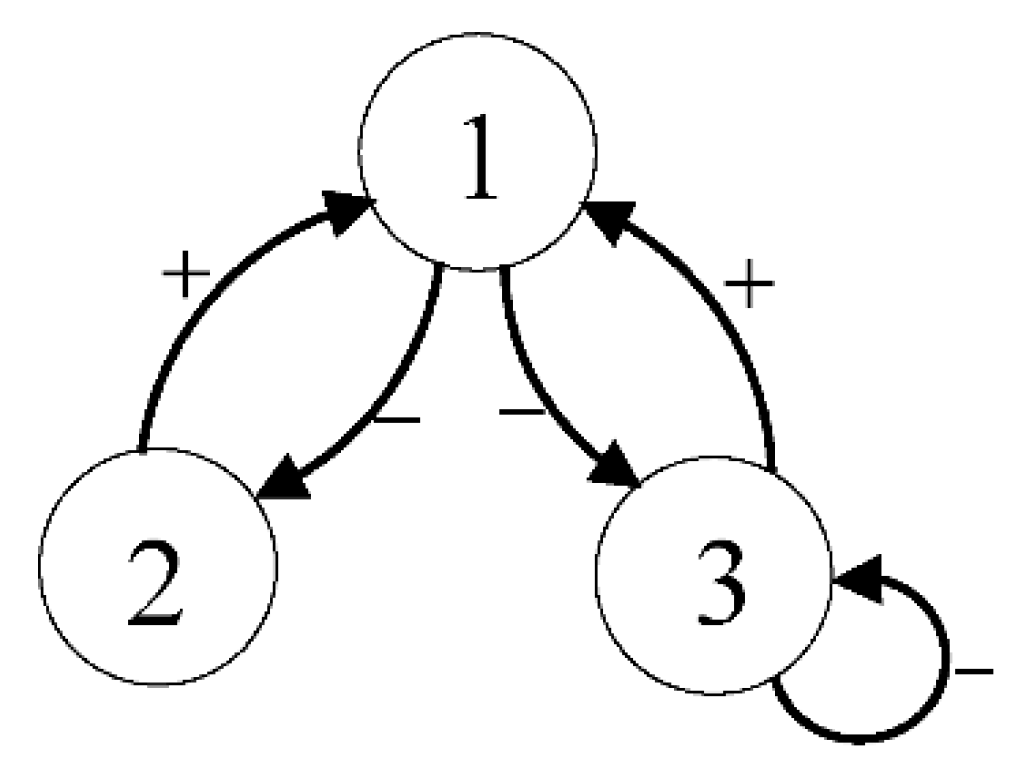
. A negative effect is designated by a negative sign. No effect is denoted by zero. A visual description of the aforementioned situation could be provided by a directed graph, which is a graph reflecting the positive or negative relationship of the elements of the sign pattern matrix. For example, assuming that the corresponding sign pattern matrices, called directed graphs, are denoted by the following:
Figure 1 depicts
’s directed graph, so
Figure 1 is called the directed graph of
.
Many researchers began to analyze sign stability and achieved great research results. Sufficiency and necessity requirements concerning the sign stability of matrices are derived by Jeffries, and the color test method to examine the sign stability for a given matrix in ecological terms is proposed [
18]. Nevertheless, the color test conditions are quite complicated for engineering problems. New necessary and sufficient conditions for sign stability were derived by some researchers [
19,
20]. Control engineering, particularly for designing robust controllers, is an area in which the sign stability approach could be employed, which is suggested by theoretical researchers. More robustness could be reached by the aforementioned approach and conservativeness is lowered when compared to the traditional Lyapunov-based stability approaches. Wang and Dong implemented the sign stability to some uncertain systems, such as flight control and switching systems, to extract sufficient and necessary requirements that lead to the sign stability concerning switched systems under a defined switching strategy [
21,
22]. An ecological sign-stability approach to construct a robust controller for linear systems was adopted by Rama who employed the sign-stability idea from ecology to develop a novel control design strategy for uncertain linear systems with robustness to a category of uncertainties in the plant parameters [
23,
24,
25]. Sign stability of linear systems is characterized by a positive Markov jump verified by sign stability to stochastic switching systems, which was applied by Cavalcanti [
26,
27].
The sign stability of dual switching linear positive systems (DSLPSs) is verified by the current research, its main contributions are: (i) the extraction of sufficient conditions so the stability of a DSLPS is guaranteed; (ii) 1-moment exponential sign stability and EMS sign stability of DSLPSs are verified. Firstly, the paper analyzes 1-moment exponential and EMS sign stability of dual switching linear continuous-time positive systems (DSLCTPSs), which depend upon the ADT and the predetermined deterministic switching strategy. Sufficiency conditions represented by LMI are then given. The sign stability analysis of DSLPS cannot be utilized by the previous strategy herein since each subsystem matrix is stable, which is not enough and is not necessary for the stability of DSLPSs. The equivalence between the stability of DSLPSs and particular matrices through LMI are also designated by our results that are similar to our previous research. Qualitative results can be of merit and an intuitive complement to conventional numerically based methods could be employed for robust stability analysis.
2. Preliminaries
The work is organized as follows. In
Section 2.1, we introduce some related mathematical concepts. In
Section 2.2, we first define the mathematical model of DSLCTPSs, 1-moment exponential stability, and EMS stability. We then use ADT and the preset deterministic switching strategy to obtain the sufficient conditions of the two kinds of stability from the sufficient condition that starts with the analysis of the equivalent condition of the corresponding sign stability. In
Section 2.3, we finally define the sign stability of DSLCTPSs.
2.1. Notation
represents the set of real matrix of dimension
, and the
-dimensional identity matrix is denoted by
. For matrix
,
denotes the element
of
, the diagonal elements
of
are denoted by
. Let
be matrices and let
be a matrix whose diagonal elements are called block diagonal.
is called the upper left block, the other diagonal block is called
, and
is called a bottom right block. Let
define a column vector whose elements equal 0 excluding the
th one that is either 1 or “+”. The other vector defined by a particular notation is
, where all elements are 1.
denotes the expansion of the column vector of
.
designates the sign of
.
and
having the same sign is denoted by equality
.
denotes the directed graph of
. For a random variable
, its expected value is denoted by
.
and
are two square matrices whose Kronecker’s product and Kronecker’s summation are expressed respectively by the following:
and
2.2. Stability of Dual Switching Linear Continuous-Time Positive Systems (DSLCTPSs)
Assume that a DSLCTPS is defined by
where the continuous state denoted by
is described by a real
-dimensional vector, a real Metzler matrix whose dimension is
(
having nonnegative values on each off diagonal) is denoted by
, such that
is positive,
evolves in the positive orthant.
denotes the deterministic switching signal whose functional form is constant and piecewise right continuous where the index of the active Markov subsystem is indicated.
for
, where switching time at instant
is denoted by
, where
and
. The switching signal defined by
denotes a function that is piecewise and constant and it is governed by an
-mode Markov process. The subscript of the active subsystem expressed by
for
is defined where
denotes the switching time at the instance
,
and
. For every
,
, called the Markov process transition probability, is defined by
when
and
,
defines the transition rate from mode
and mode
at the times
and
, respectively
where
denotes the transition rate matrix of
.
, called the Markov process, is considered irreducible if
. Thus, it is called ergodic and its unique invariant distribution
satisfies
The increased time stays in the subsystem of in and is denoted by and the subsystem’s incident number of in is denoted by .
Lemma 1. (Ref. [
8]
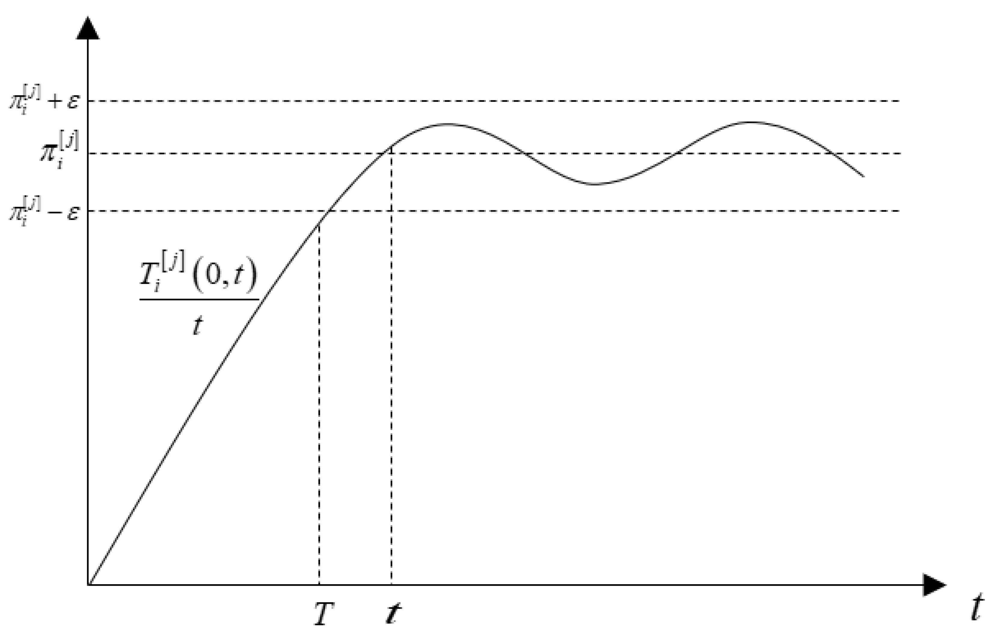
) For any , , an N-mode Markov process for is assumed. The Markov process whose transition rate matrix and stationary distribution are denoted by and , respectively. Then, for and , the probability equation is defined by and Remark 1. For, there is a positive constant that meetsand Proof. From (6),
, while
,
, as shown in
Figure 2, then
. For different
, there are corresponding
, so while
,
. The same is true for (8). □
Definition 1. (Ref. [
2]
) System (1) is characterized by the -moment exponential stability if the following inequality is satisfied by positive real parameters of and when and represent all positive initial conditions and all initial probability distributions. When and , the above definition is compatible with the well-known notion of 1-moment exponential stability and exponential mean-square stability (EMS stability), respectively.
Definition 2. (Ref. [
4]
) For any deterministic switching signal and all , the number of the deterministic switching signals occurring in the interval is denoted by and the ADT of the deterministic switching signal during is denoted by . A positive number , called the chatter bound, exists such that it satisfies Theorem 2. Consider the DSLCTPS (1). Assume that strictly positive vectors exist such that wheresuch that the inequalities given below hold:Now, system (1) is 1-moment exponentially stable when the ADT of the deterministic switching signal satisfies Theorem 3. When the ADT of the deterministic switching signal satisfiesof Theorem 2, andmeets, the system (1) meets 1-moment exponential stability if and only ifmeets the Hurwitz stability: Proof. Let
, because
, which is derived from
of Theorem 2, then
(9) allows
of Theorem 2 to hold. Thus,
It can guarantee that
and
of Theorem 2 have solutions. If (10) holds, then
when (11) is only a necessary condition. Let
, then
and
are sign equivalent.
Let . It is immediate to verify that the previous inequation in (11) can be rewritten as , since is a Metzler matrix there is a strictly positive vector that meets if and only if meets the Hurwitz stability.
Since (12) and (13) are sign equivalent, system (1) is 1-moment exponentially stable; that is, meets the Hurwitz stability. □
Theorem 4. Assume system (1). Assume that there are symmetrically positive definite matrices, which satisfy the following inequalities:Now, system (1) is EMS stable under the upcoming switching mechanismwhere the SS of the switching signal is determined deterministically, inis denoted by as the switching subscript sequence of the switching signal determined deterministically and is denoted by Theorem 5. Consider the deterministic switching strategy of Theorem 4, whileallowsto hold, the system in (1)
meets EMS stability if and only if is Hurwitz stable. Proof. Let
Considering
of Theorem 4, then
Satisfies
of Theorem 4. From (14), then
The inequation in (16) proves the necessary condition. As
,
and
are sign equivalent. Using
, from (16), we obtain
Hence, (19) can be expressed as
if there are symmetrically positive definite matrices
, equivalently, if and only if
has the Hurwitz stability property.
Since (17) and (18) are sign equivalent, the system in (1) is EMS stable, equivalently, if and only if is Hurwitz stable. □
2.3. Qualitative Characterization of Dual Switching Linear Continuous-Time Positive Systems
The assumption in this research is that the numerical realization of and are not known. and belong to a class of structured matrices whose elements contain given signs. A matrix with signs is defined where all elements are represented by signs belonging to . The set of sign matrices whose orders are by is denoted by . Matrices consisting of real numbers with specific classifications agree upon are inherently compatibility with the above matrices where their features are not related to the elements that have special values.
A corresponding unique sign matrix can be constructed by allocating a member of the set to its elements based on its sign for a given matrix . Due to having a similar sign matrix assigned by two different real matrices, the class of whole matrices consisting of real numbers corresponding to a sign matrix can be defined as follows.
Definition 3. (Ref. [
20]
) The qualitative group of the matrix consisting of real numbers whose order in n by m can be defined by A unique qualitative group for each sign matrix can be observed. Suppose that
designates the qualitative class
, where
holds for some matrix
consisting of real numbers with proper dimension for a certain sign matrix
. Correspondingly
and
for a sign matrix
whose order is N by N. Note that if
, then
is an empty set.
Table 1 presents the definitions of the aforementioned sets.
Subsystem matrices whose given structures are known can be expressed by corresponding sign matrices. Therefore, the definition of the system denoted by (1) is expressed as follows:
In the above relation, all are unknown but belong to the pre-defined qualitative classes and .
Definition 4. (Ref. [
26]
) If there is in and in such that system (1) is 1-moment exponentially stable or EMS stable, then (21) is called 1-moment exponentially sign stable or EMS sign stable.
3. Sign Stability Concept
A variety of subsystem prototypes defined by sign matrices , to express various qualitative classes, is admitted by System (21). should be generalized to tackle the ambiguity led by sign matrices with various nonzero elements. Therefore, some subsystem structures in (21) can be embedded into a single matrix.
Definition 5. (Ref. [
21]
) The matrix is sign stable if every matrix with a similar sign pattern to is Hurwitz stable, regardless of the values of .
Definition 6. If satisfies for all sequences with two or more different indices , then is called acyclic.
Theorem 6. (Ref. [
20]) All of these declarations are equivalent:
is acyclic;
There is a permutation matrixwhereis upper triangular.
Definition 7. (Ref. [
21]
) The joining operation of each sign pattern can be defined to establish a particular sign pattern called the initial sign pattern of the set based on the isogenous term set, the mentioned steps satisfy the conditions below. (1) For a specific location of any sign pattern whose elements are denoted by 0 or the nonzero sign, the corresponding ones in the original sign pattern can be composed of a similar nonzero sign.
(2) For a specific location of any sign pattern whose elements are all equal to 0, the corresponding one in the original sign pattern is also 0.
(3) For a specific location of any sign pattern whose elements consist of distinct signs, the corresponding ones in the initial sign pattern should be employed to define all possible signs, “”. A bounded set of sign matrices is considered, the original sign pattern is expressed as .
For example, if
then, its original sign pattern is
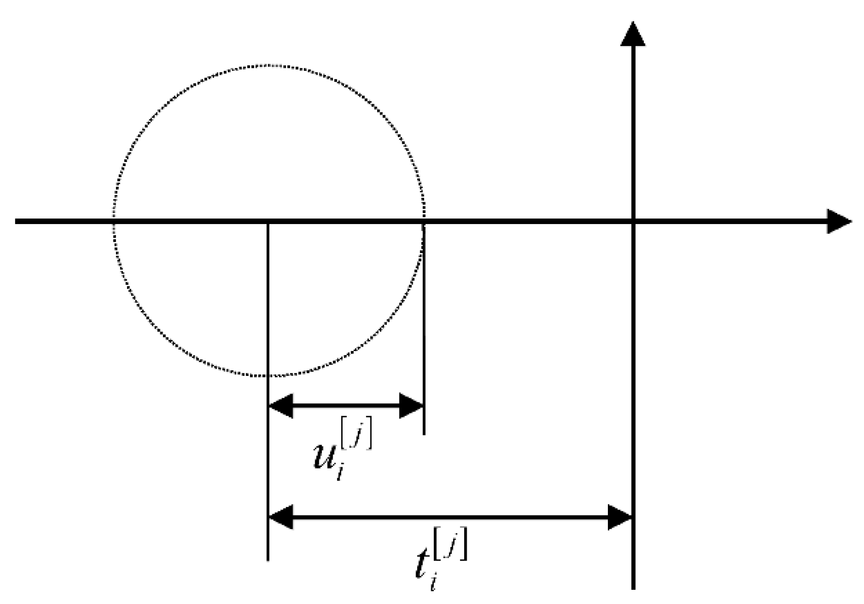
Theorem 7. (Gershgorin’s Circle Theorem)
Each eigenvalue of the n-order matrix is located in the following n circles Gershgorin’s Circle Theorem used in this paper is a relatively conservative theorem. In the analysis of sign stability the boundary of the circle is not discussed, only the eigenvalues contained in the circle are analyzed. The problem of the boundary of the disc needs further discussion.
Theorem 8. (Ref. [
18]
) Assume that could be a partitioned matrix whose partitions are denoted by , with the property that , then is called sign stable, if and only if each partition matrix is sign stable.
4. 1-Moment exponential Sign Stability and EMS Sign Stability
The sign matrices
and
of the DSLCTS (21) are considered. The representative matrix
is denoted by
and
is expressed by
where
denotes the expanded parallel sign matrix
consisting of real numbers, where its graph reflects how the graph
interconnects and meshes with particular subsystems when the DSLCTS is a concern.
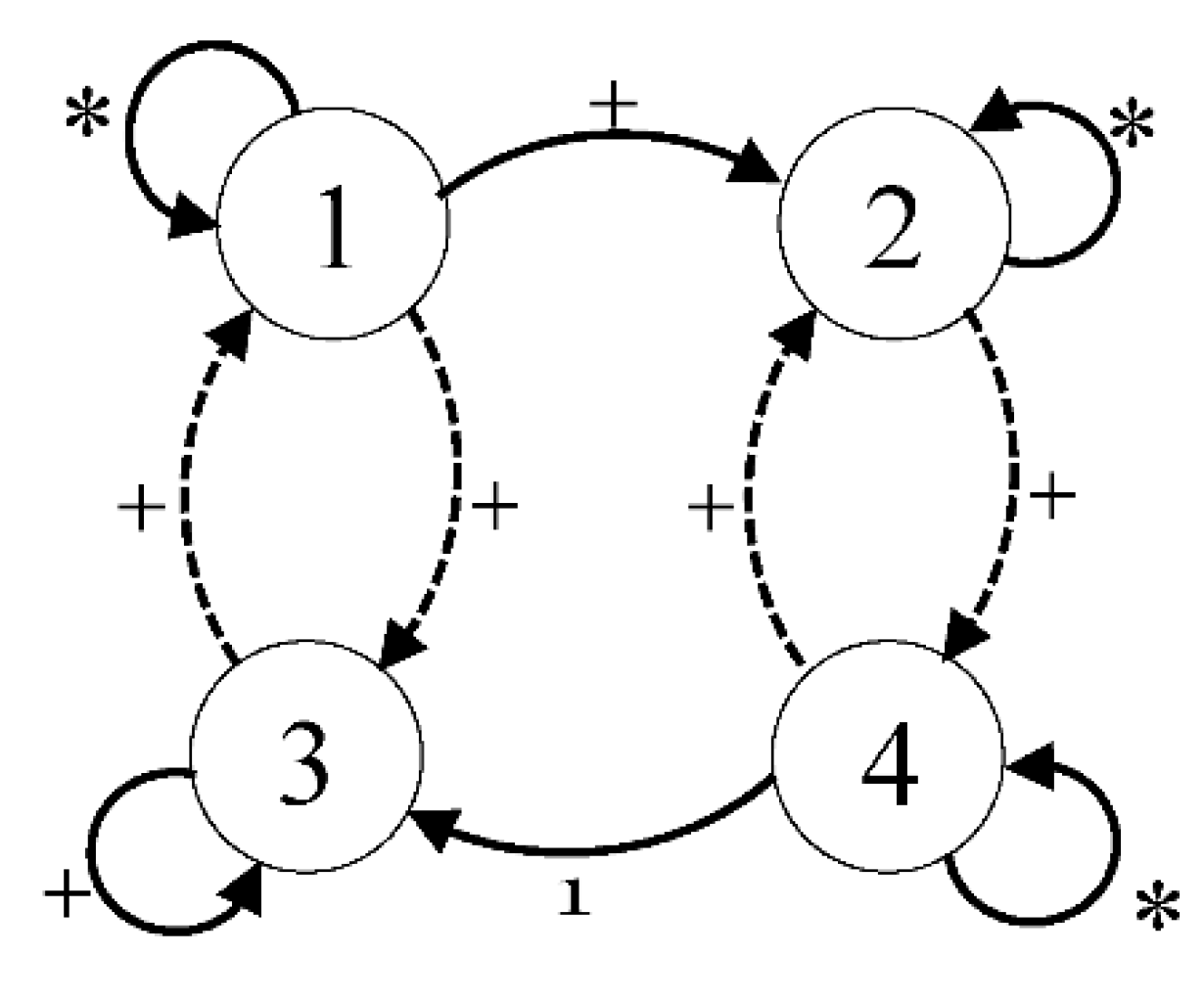
To clarify the mentioned interaction, assume (21) with
then
can take the form given below utilizing the case above
Figure 3 depicts
’ s directed graph. In
, the graph
adjoins the above two acyclic graphs. The sign stability
is verified by analyzing the relationship of
,
, and
.
4.1. 1-Moment Exponential Sign Stability Analysis
Theorem 9. Assume that the class of sign matrices is represented by. . The representations below are mathematically equal:
is sign stable;
is acyclic,.
Proof. Consider that
is an
permutation matrix, where
is an
matrix with the canonical column vectors
as its columns; that is,
and
such that
,
,
As
is acyclic,
is acyclic by Definition 7. Therefore, a permutation matrix
exists where
is upper triangular by Theorem 6 and one of
and
are zero matrices. Since
inherits graphical properties
is a permutation matrix
such that
is triangular matrix whose entities are located at the upper block and its block-diagonal matrices were
. The process is as follows.
is a matrix where all of its elements are 0,
is
or
, which is not a matrix with all zero elements. If
is sign stable, equivalently,
is sign stable, equivalently,
is sign stable. Moreover,
is sign stable if and only if all
are sign stable by Theorem 8.
Since
, then
Because
and
,
,
. Now, according to Theorem 7 and Definition 5,
,
as shown in
Figure 4. Thus,
are sign stable, leading to sign stability of
. □
Theorem 10. When the ADT of the deterministic switching signal satisfiesof Theorem 2, andallowsto hold, if for each, satisfies Theorem 9, then the system (21) is 1-moment exponentially sign stable.
Proof. When the ADT of the deterministic switching signal satisfies of Theorem 2, and makes hold, system (1) meets 1-moment exponential stability if and only if is Hurwitz stable by Theorem 3. According to Definition 4, if system (1) is 1-moment exponentially stable, and every belongs to and belongs to , then (21) is 1-moment exponentially sign stable. Thus, every belongs to and belongs to , such that is sign stable, leading to 1-moment exponential sign stability of (21). Then, for each , satisfies Theorem 9, and the system (21) is 1-moment exponentially sign stable. □
4.2. EMS Sign Stability Analysis
Theorem 11. Assume that the set of sign matricesare represented by. The representations below are mathematically equal:
is sign stable;
is acyclic,.
Proof. Since
is acyclic,
is also acyclic by Definition 7; that is,
,
Thus,
inherits the graphical properties of
,
is acyclic, and
stands for the extended sign matrix analogue of the real matrix
inherits the graphical properties of
, and
and we only prove that
is sign stable.
Because
, then
Since and , , , and . According to Theorem 7 and Definition 5, is sign stable. □
Theorem 12. Under the deterministic switching strategyof Theorem 4, whileallowsto hold, ifandsatisfies Theorem 11, the system in (21) is EMS signstable.
Proof. The proof is similar to that of Theorem 10. □
Theorem 13. For the system in (21), 1-moment exponential sign stability and EMS sign stability are sign equivalent.
Proof. From Theorem 9 and Theorem 11, if and are sign stable, then and . Since , . All are acyclic because is acyclic and all are Metzler matrices. Thus, for a DSLCTSs (21), 1-moment exponential sign stability and EMS sign stability are sign equivalent. □
5. Sign Example and Numerical Example
For 1-moment exponential sign stability and EMS sign stability, let .
In order to satisfy condition
of Theorem 9 and Theorem 11, select the original sign pattern as
.
Then, choose the sign matrices arbitrarily in as the sign matrices of the subsystem.
For example,
Assume the corresponding generators of the Markov switching signals
and
as
The invariant distributions are
,
. The initial condition is chosen as
. The other parameters are shown in
Table 2.
For 1-moment exponential sign stability, , the ADT of 1-moment exponential sign stability is ; for EMS sign stability, . The numerical verification of the 1-moment exponential stability and EMS stability follows.
Is used to assess the 1-moment exponential stability
, is used to assess the EMS stability.
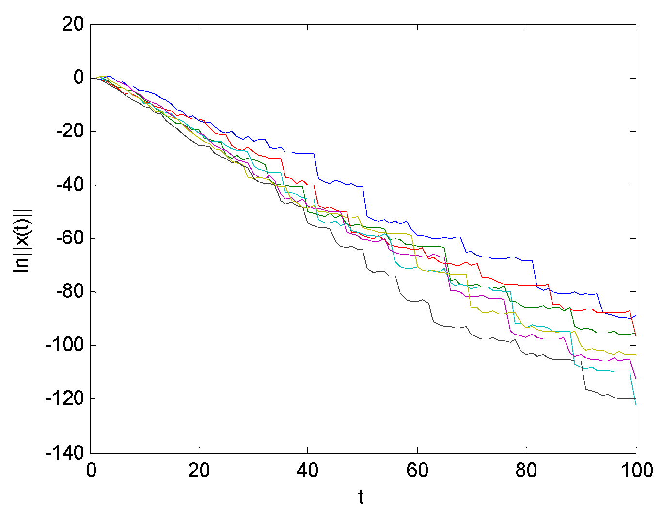
Example 1. 1-moment exponential stability.
Substituting the numerical values to verify the 1-moment exponential stability.
Let
, solving
,
, and
of Theorem 2 gives
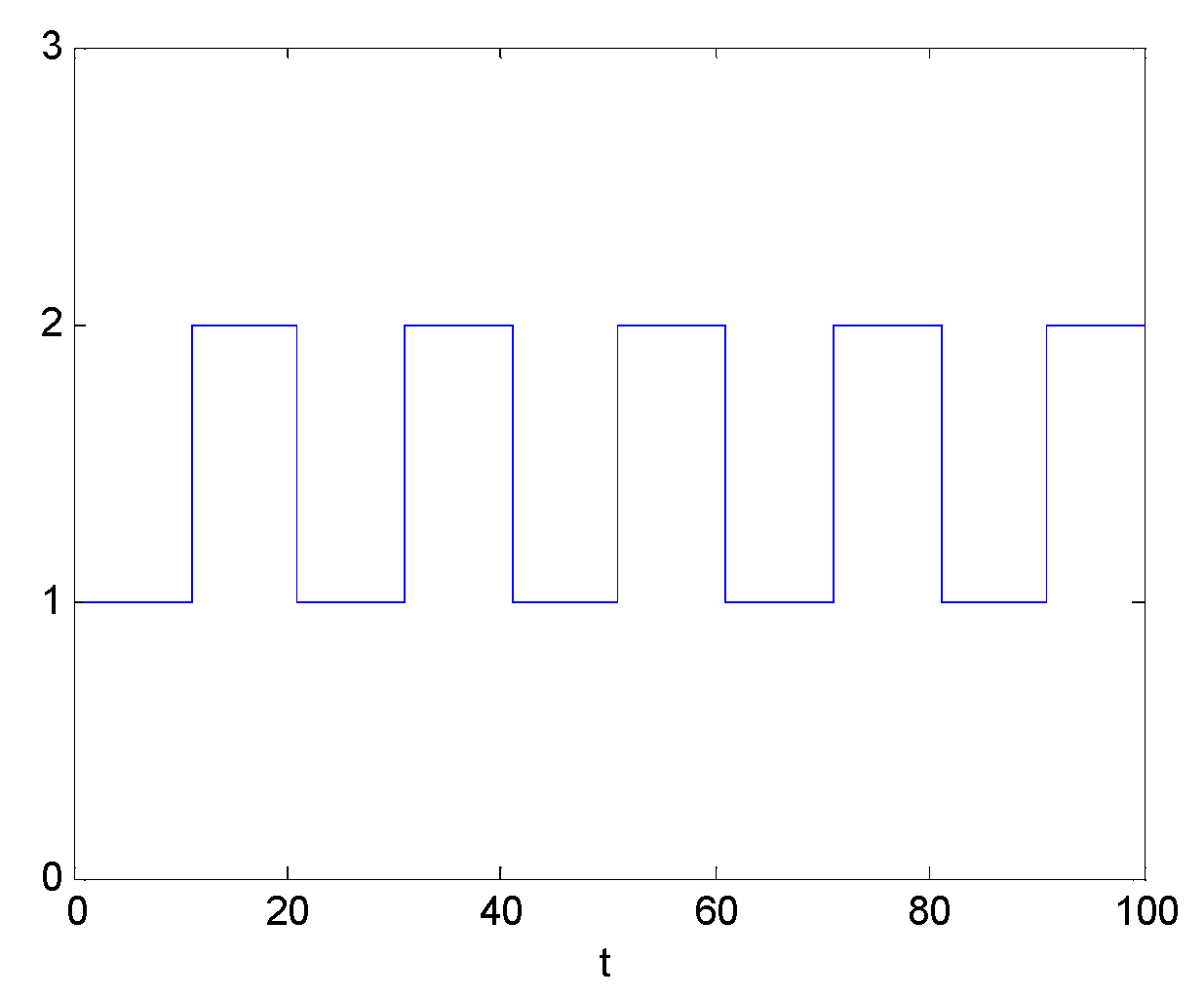
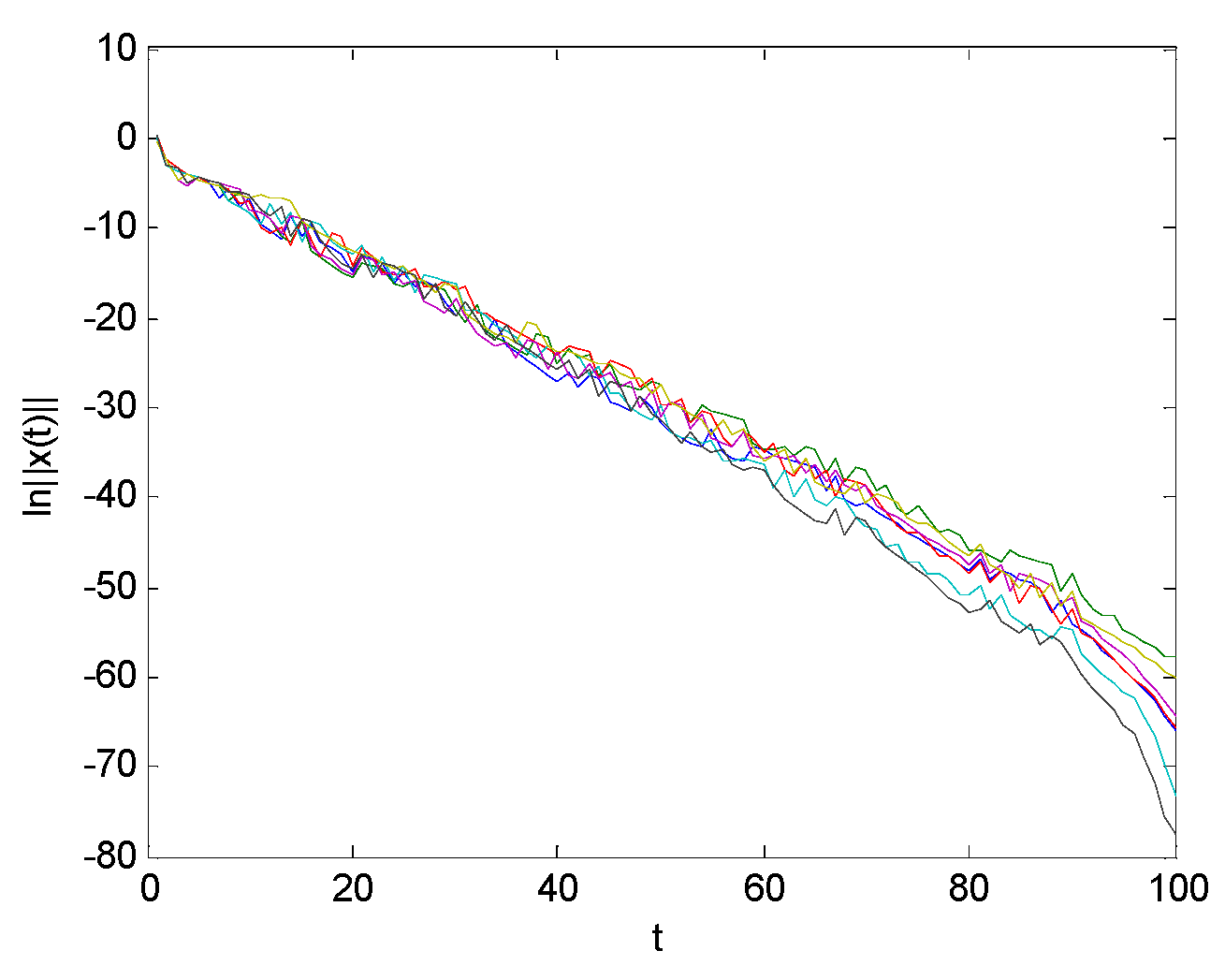
Figure 5 and
Figure 6 present the ADT
and the state trajectories, respectively.
Example 2. 1-moment exponential unstability.
Substituting the numerical values to make the first subsystem ineligible.
Let
,
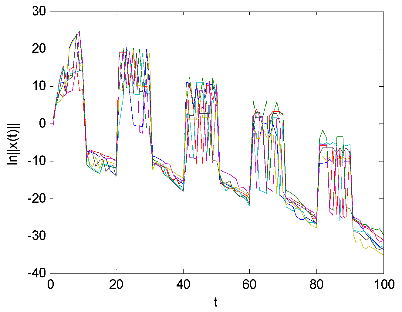
Figure 5 and
Figure 7 present the ADT
and the state trajectories, respectively.
Because the first subsystem matrices do not meet the conditions, when switching to the first subsystem it can be seen from
Figure 7 that the state trajectories are unstable.
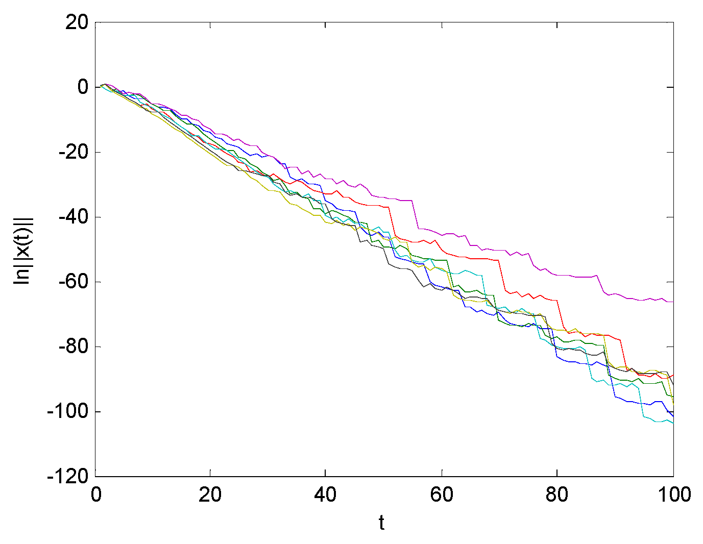
Example 3. EMS stability.
Substituting the numerical values to evaluate the EMS stability.
Solving
and
of Theorem 4 yields
Figure 8 and
Figure 9 give the deterministic switching signal
and the state responses, respectively.
Example 4. EMS stability without the deterministic switching.
Substituting the numerical values to make the second subsystem ineligible
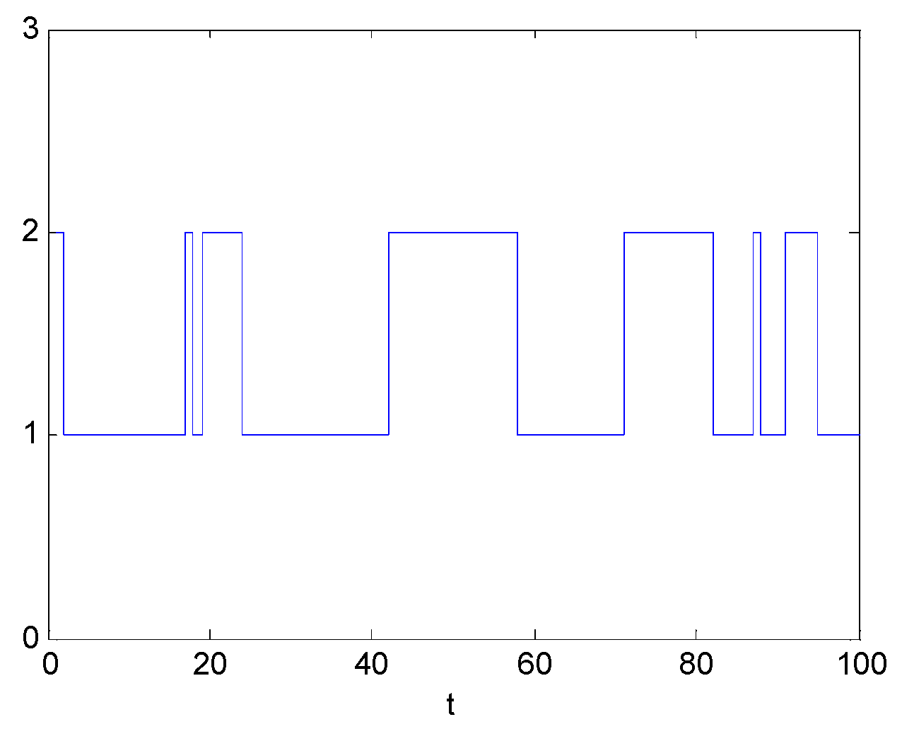
Figure 10 and
Figure 11 give the deterministic switching signal
and the state responses, respectively.
Because the second subsystem matrices do not meet the conditions, according to preset deterministic switching strategy, it can be seen from
Figure 10 that the system only runs on the first stable subsystem.


