Symbol Error-Rate Analytical Expressions for a Two-User PD-NOMA System with Square QAM

Abstract

Power domain non-orthogonal multiple access (PD-NOMA) is one of the most perspective multiplexing technologies that allows improving the capacity of actual networks. Unlike orthogonal multiple access (OMA), the PD-NOMA non-orthogonally schedules multiple users in the power domain in the same orthogonal time-spectrum resource segment. Thus, a non-orthogonal multiplexed signal is a combination of several user signals (usually, modulation and coding schemes (MCS) based on quadrature amplitude modulation) with different power weights. The symbol error rate (SER) and bit error rate (BER) performances are one of the main quality characteristics of any commutation channel. The issue is that a known analytical expression for BER and SER calculation for conventional OMA cannot be applied in terms of the PD-NOMA. In the following work, we have derived the SER and BER analytical expressions for gray-coded square quadrature amplitude modulation (QAM) user channels that are transmitted in two-user PD-NOMA channel under additive white Gaussian noise (AWGN). Through the simulation, the verification of the provided expressions is presented for four multiplexing configurations with various user power weights and QAM order combinations.

1. Introduction

The power domain non-orthogonal multiple access (PD-NOMA) is a perspective technology for user multiplexing in future networks [1,2,3,4,5,6,7]. It is based on non-orthogonal channel multiplexing by user signal superposition in the power domain at the same time-frequency resource segment (for example, a subcarrier in orthogonal frequency division multiplexing). Thus, there is a controlled co-channel interference which is cancelled at the receiver side by the successive interference cancellation (SIC) method [8] in the SIC detector. In comparison to orthogonal multiple access (OMA), such as orthogonal frequency division multiple access (OFDMA), the PD-NOMA exploits the channel state differences between users. Thus, the available power of a resource segment is divided between multiplexed users, according to the required quality of the service and channel state information of each user. Therefore, resource allocation occurs in power, frequency, and time domains simultaneously. Due to the non-orthogonal power allocation techniques, the spectral and energy efficiency advantages of multiuser communication systems can be obtained.

There is a significant number of PD-NOMA articles; most of them are aimed at the design of new analytical resource scheduling [9,10,11,12,13,14,15] and research of system gains in comparison to OMA systems [16,17]. Mostly, these results are based on the Shannon–Hartley theorem [18] and do not take into account bit error rate (BER) and symbol error rate (SER) performances, which are different from OMA systems. However, it is necessary to consider BER and SER to obtain a more reliable result because the BER and SER are the main performance parameters of real signals in an additive white Gaussian noise (AWGN) channel. Usually, the signal construction based on quadrature amplitude modulation (QAM) is used in both OMA and PD-NOMA. However, there is an issue that the analytical expressions for calculating the error probability are not equal. Those expressions are given in [19] for OMA. For the PD-NOMA, this issue has not been well-studied, and only a few works provide a solution for these problems.

The SER and BER analysis using SIC detectors has received attention in recent works. In [20], the BER is explored for PD-NOMA under Rayleigh fading channel where exact and approximate expressions are obtained. However, the presented expressions are applicable only for two-user PD-NOMA with binary phase shift keying (BPSK) and quadrature phase shift keying (QPSK). The BER expressions over Nakagami-m channel for two and three-user scenarios using QPSK are derived in [21]. In [22], the authors present BER expressions for PD-NOMA systems while using only QPSK in both user channels. Work [23] also considers the study of SER and BER in PD-NOMA systems, and the authors present a closed-form expression within the conditions of Gray coding and QPSK. In [24], the researchers study the analytical SER in visible light communication systems with the NOMA; however, QAM is not considered. SER expression using QAM is presented in [25] which has non-ideal accuracy for the second non-orthogonal layer. As can be seen from the discussion above, there is no paper that considers the exact SER expressions of toe first and second non-orthogonal user in PD-NOMA with square QAM.

The purpose of our work is to derive the analytical SER and BER expressions for a two-layer PD-NOMA system under the conditions of square QAM multiplexing. First of all, we describe a two-layer PD-NOMA system model and known expressions for conventional square QAM in the OMA system. Secondly, we give SER and BER expressions for a QAM signal in the first and second non-orthogonal layers consistently. Finally, the simulation and analytical calculation results of BER and SER are compared.

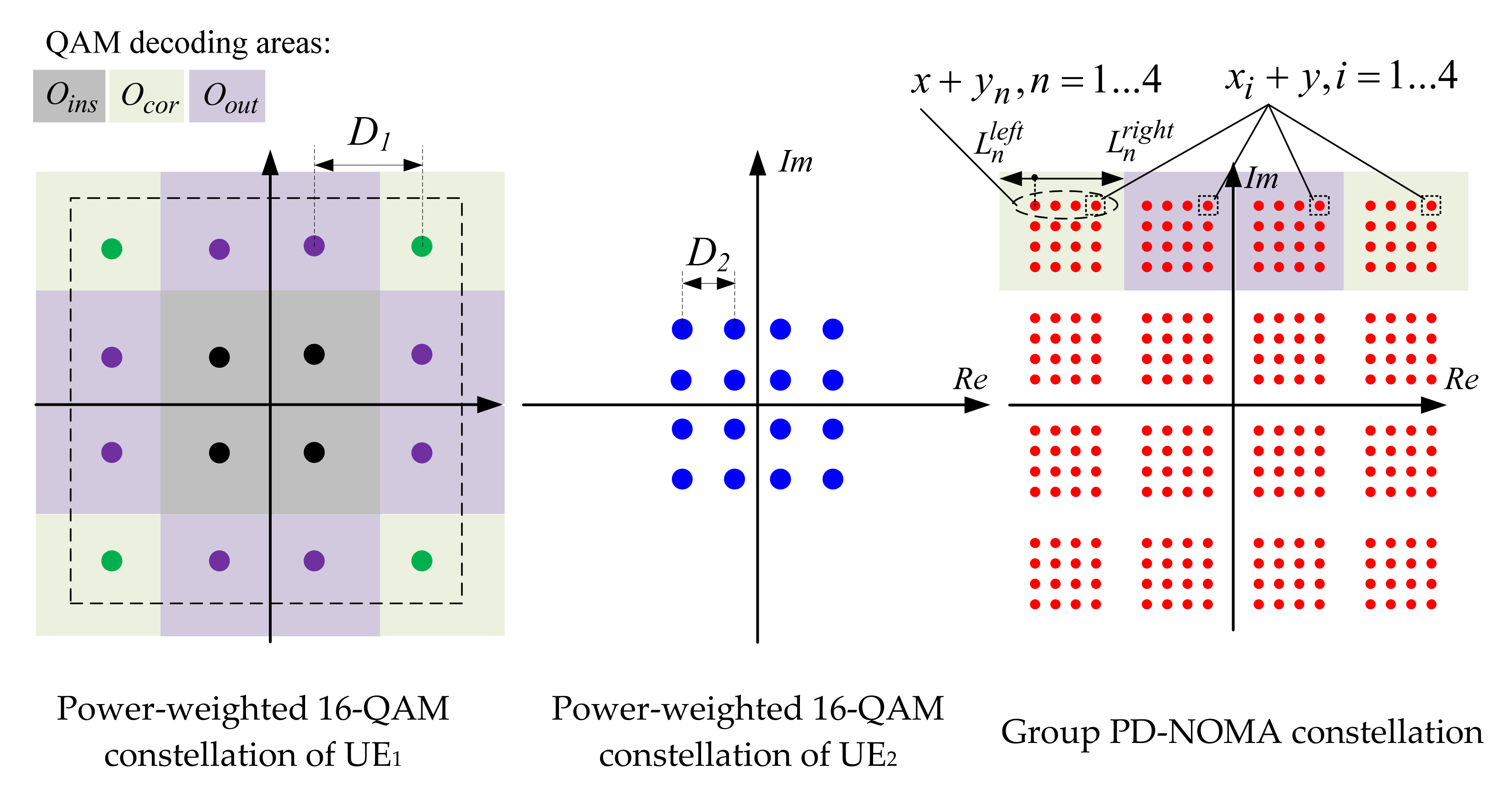
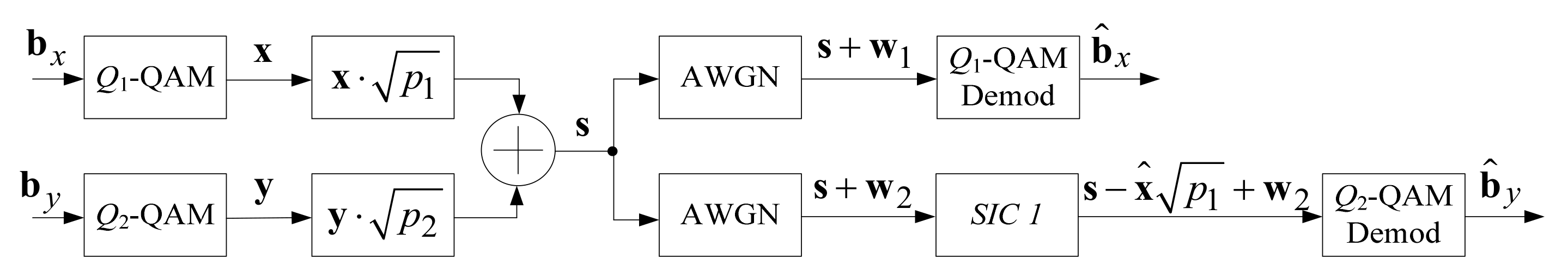
2. System Model

Our work considers only the two-layer PD-NOMA multiplexing in the downlink. The PD-NOMA system model includes a one-base station (BS), two user’s equipments (UE₁ and UE₂), and AWGN channel propagation between them. The downlink group signal s at BS output is given by the superposition of two user signals according to

$$s=\sqrt{p_1}x+\sqrt{p_2}y,$$

(1)

where x and y are the modulation symbols, and $p_1,p_2$ are the power weights of UE₁ and UE₂. The total power of the output signal is $E_s=p_1+p_2$. We use a typical scenario for the PD-NOMA that UE₁ and UE₂ are located far from the BS and near it. In this scenario, the channel state of UE₁ is worse compared to UE₂; therefore, $p_1>p_2$. We assume that users utilize signal constructions based on Gray coding and square QAM with the modulation orders $Q_1{Q}_2\in 2^R$ ($R=2t$ (bits/symbol), $t\in \mathbb{N}$). The possible states of x and y are given by the alphabets $A_1$ $(x\in A_1)$ and $A_2$ $(y\in A_2)$. Figure 1 offers an example of two 16-QAM (Q₁, Q₂ = 16) user constellations and the superposed PD-NOMA constellation. The minimum Euclidean distance $D_k$ between the nearest points on the power-weighted constellation of UE_k is given by

$$D_k=2\sqrt{\frac{p_k}{M_k}},$$

(2)

where $M_k=2/3\times (Q_k-1)$ is the normalization factor.

The group signal is transmitted to users via the AWGN channel with a complex additive noise $w~CN(0,N_0)$ that follows the Gaussian probability distribution function with zero mean and noise power spectral density $N_0$. The PD-NOMA symbol received by the one of the users is given by

$$s=\sqrt{p_1}x+\sqrt{p_2}y+w.$$

(3)

To decode a PD-NOMA symbol, the successive interference cancellation (SIC) method is employed. Thus, the symbol x is decoded from the first non-orthogonal layer by the minimum Euclidean distance criterion from s and by treating y as interference. It can be expressed as

$$\widehat{x}=arg\underset{x\in A_1}{min}{\left|s-\sqrt{p_1}x\right|}^2.$$

(4)

Then, the symbol y is decoded from the second non-orthogonal layer using SIC by following these three steps. Firstly, the symbol x is decoded by treating its own symbol y as the interference. Secondly, the decoded symbol $\widehat{x}$ is cancelled from s as follows: $s\prime =s-\sqrt{p_1}\widehat{x}$. Finally, its own symbol y is decoded from $s\prime$ by

$$\widehat{y}=arg\underset{y\in A_2}{min}{\left|s\prime -\sqrt{p_2}y\right|}^2.$$

(5)

3. BER and SER for Conventional Square QAM Signal

First, we shortly describe a conventional square QAM decoding process and show the known analytical SER and BER over the $E_s/N_0$ expressions for it. Let the received square Q-QAM symbol be $u=u\prime +w$, where $u\prime$ is the transmitted symbol using alphabet $A$ $(u\prime \in A)$, and w is the AWGN realization. The receiver decodes u by the minimum Euclidean distance criterion as follows

$$\widehat{u}=arg\underset{u\prime \in A}{min}{\left|u-u\prime \right|}^2.$$

There are Q possible states on the Q-QAM constellation, which can be divided into three groups: corner, inside, and outside symbols. It is observed on the 16-QAM constellation of UE₁ shown in Figure 1. Thus, let $\rho \left(u_{cor}\right)$, $\rho \left(u_{ins}\right)$, $\rho \left(u_{out}\right)$ be occurrence probabilities, and $\rho \left(\overline{u}\right|u_{cor})$, $\rho \left(\overline{u}\right|u_{ins})$, $\rho \left(\overline{u}\right|u_{out})$ be error decoding probabilities of the corner, inside, and outside symbols. Next, we obtain the symbol error probability $\rho \left(\overline{u}\right)$ as follows

$$\rho \left(\overline{u}\right)=\rho \left(u_{cor}\right)\rho \left(\overline{u}\right|u_{cor})+\rho (u_{ins}\left)\rho \right(\overline{u}\left|u_{ins}\right)+\rho \left(u_{out}\right)\rho \left(\overline{u}\right|u_{out}),$$

(6)

where occurrence probabilities are known from the ratio number of each type of symbol position to the constellation order Q and given by

$$\begin{array}{l}\rho \left(u_{cor}\right)=\frac{4}{Q}\\ \rho \left(u_{ins}\right)=\frac{Q-4(\sqrt{Q}-1)}{Q}\\ \rho \left(u_{out}\right)=\frac{4(\sqrt{Q}-2)}{Q}\end{array}$$

(7)

The corner, inside, and outside symbols have different correct decoding areas. The calculation of the decoding probabilities is based on obtaining the detecting areas and the probability u that falls outside due to AWGN with the $E_s/N_0$ ratio. The derivation of the analytical expressions for the error decoding probabilities of the square QAM is well-described in [26]. We introduce these expressions below

$$\begin{array}{l}\rho (\overline{u}|u_{cor})=erfc\left(\sqrt{\frac{E_s}{M{N}_0}}\right)-\frac{1}{4}erf{c}^2\left(\sqrt{\frac{E_s}{M{N}_0}}\right)\\ \rho (\overline{u}|u_{ins})=2erfc\left(\sqrt{\frac{E_s}{M{N}_0}}\right)-erf{c}^2\left(\sqrt{\frac{E_s}{M{N}_0}}\right)\\ \rho (\overline{u}|u_{out})=\frac{3}{2}erfc\left(\sqrt{\frac{E_s}{M{N}_0}}\right)-\frac{1}{2}erf{c}^2\left(\sqrt{\frac{E_s}{M{N}_0}}\right)\end{array}$$

(8)

where $erfc(x)$ represents the complementary error function, which is defined as $erfc(x)=\frac{2}{\sqrt{\pi }}{\displaystyle \underset{x}{\overset{\infty }{\int }}{e}^{-x^2}}dx$.

The common probability of error decoding $\rho \left(\overline{u}\right)$ in the AWGN channel with the $E_s/N_0$ ratio is obtained by putting (7) and (8) into (6) and simplifying the resulting expression as follows

$$\rho (\overline{u})=2\left(1-\frac{1}{\sqrt{Q}}\right)erfc\left(\sqrt{\frac{E_s}{M{N}_0}}\right)-\left(1-\frac{2}{\sqrt{Q}}+\frac{1}{Q}\right)erf{c}^2\left(\sqrt{\frac{E_s}{M{N}_0}}\right),$$

(9)

Finally, the BER value ${\rho }_b\left(\overline{u}\right)$ can be obtained under the same conditions by averaging the result of (9) with help of $lo{g}_{2}Q$ by

$${\rho }_b(\overline{u})\approx \frac{\rho \left(\overline{u}\right)}{lo{g}_{2}Q}.$$

(10)

4. BER and SER for PD-NOMA Square QAM Signal

Now, let us derive analytical expressions for SER and BER against the $E_s/N_0$ ratio in the PD-NOMA scenario. We consider that the first layer receives the largest power portion $p_1$ of the total transmit power $E_s$, and the second layer receives the remainder $p_2=E_s-p_1$. According to the SIC, the first layer is decoded in the first instance, considering that the second layer and AWGN are interferences. The second layer is decoded under the conditions of AWGN only after the perfect interference cancellation of the first layer; however, the incorrect cancellation causes the additional signal corruption. Further, we describe the signal decoding process in both PD-NOMA layers and get BER and SER expressions for them.

4.1. First Layer Decoding

The received PD-NOMA symbol s is expressed in (3), where the information symbol x of UE₁ is transmitted in the first non-orthogonal layer. Denote $\rho \left(\overline{x}\right)$ and ${\rho }_b\left(\overline{x}\right)$ as symbol and bit error probabilities while decoding x from s. Similar to conventional QAM, we define three types of the received symbols: the corner symbol $s_{cor}$ contains corner symbol $x_{cor}$; $s_{ins}$ contains $x_{cor}$, and $s_{out}$ contains $x_{out}$. The occurrence probabilities are the same as for QAM, and they can be obtained from (7) by

$$\begin{array}{l}\rho (s_{cor})=\frac{4}{Q_1}\\ \rho (s_{ins})=\frac{Q_1-4({\sqrt{Q}}_1-1)}{Q_1}\\ \rho (s_{out})=\frac{4({\sqrt{Q}}_1-2)}{Q_1}\end{array}$$

(11)

Then, $\rho \left(\overline{x}\right)$ is obtained by using the same ideas as in (6) and given by

$$\rho \left(\overline{x}\right)=\rho \left(s_{cor}\right)\rho \left({\overline{x}}_{cor}\right|s_{cor})+\rho (s_{ins}\left)\rho \right({\overline{x}}_{ins}\left|s_{ins}\right)+\rho \left(s_{out}\right)\rho \left({\overline{x}}_{out}\right|s_{out}),$$

(12)

where $\rho \left({\overline{x}}_{cor}\right|s_{cor})$, $\rho \left({\overline{x}}_{ins}\right|s_{ins})$, $\rho \left({\overline{x}}_{out}\right|s_{out})$ are the probabilities of the error decoding $x_{cor}$, $x_{ins}$, $x_{out}$ from $s_{cor}$, $s_{ins}$, $s_{out}$. In turn, the probability of the error decoding for $\forall x\in A_1$ is given by $\rho \left(\overline{x}\right|s)=1-\rho (x\left|s\right)$, where $\rho \left(x\right|s)$ is the probability of the correct decoding x. Further, the symbol x is decoded correctly when the real and imaginary components of s fall into its own decoding area. Let ${\Re }_s$ and ${\Im }_s$ be the real and imaginary components of s, then $\rho \left(x\right|s)$ is calculated by

$$\rho \left(x\right|s)=\rho ({\Re }_s\in O_x)\times \rho ({\Im }_s\in O_x),$$

(13)

where $O_x$ is the decoding area of x.

The symbol x can be simultaneously combined with $\forall y\in A_2$; thus, we denote $x+y_n$ as the combination presented in one region (real or imaginary) for $n=1\dots \sqrt{Q_2}$. For example, $x+y_n$ in the real region are shown on the group constellation in Figure 1. Further, we focus on the real region and ${\Re }_s$. Thus, let us note the equation for $\rho ({\Re }_s\in O_x)$ as follows

$$\rho ({\Re }_s\in O_x)={\displaystyle \sum _{n=1}^{\sqrt{Q_2}}\rho (x+y_n)\times \rho ({\Re }_{x+y_n}\in O_x)},$$

where $\rho (x+y_n)$ is the occurrence probability of the $x+y_n$ combination, and $\rho ({\Re }_{x+y_n}\in O_x)$ is the probability that the real component of $x+y_n$ falls into $O_x$. The occurrence probabilities are equal for all the combinations; therefore, $\rho (x+y_n)=1/\sqrt{Q_2}$. Then, the expression for $\rho ({\Re }_s\in O_x)$ can be rewritten by

$$\rho ({\Re }_s\in O_x)=\frac{1}{\sqrt{Q_2}}{\displaystyle \sum _{n=1}^{\sqrt{Q_2}}\rho ({\Re }_{x+y_n}\in O_x)}.$$

(14)

Now, we need to obtain the probabilities for the corner, inside, and outside symbols, using (14), and put them in (12). Firstly, we obtain the expression for finding the correct decoding probability for $x_{ins}$. The decoding area $O_{ins}$ is limited by two sides in the real and imaginary regions (Figure 1) equally, so, using (13), we have $\rho (x_{ins}|s_{ins})=\rho {(R_{s_{ins}}\in O_{ins})}^2$. In turn, $\rho ({\Re }_{s_{ins}}\in O_{ins})$ is obtained by (14). As we can see, it is enough to find $\rho ({\Re }_{x_{ins}+y_n}\in O_{ins})$ and substitute it to (14).

The Euclidian distance from the reference constellation point $\sqrt{p_1}{x}_{ins}+\sqrt{p_2}{y}_n$ to the left bound of $O_{ins}$ is

$$L_n^{left}=\frac{1}{2}\left[D_1-\left(\sqrt{Q_2}-2n+1\right)D_2\right],$$

(15)

and to the right bound is

$$L_n^{right}=\frac{1}{2}\left[D_1+\left(\sqrt{Q_2}-2n+1\right)D_2\right].$$

(16)

where $D_1$ and $D_2$ are obtained by (2). Note that $L_n^{left},L_n^{right}>0\forall n$; otherwise, the power weight ratio $p_1/p_2$ is unallowable, and the PD-NOMA signal is formed wrong.

The reference constellation point $x_{ins}+y_n$ is between $L_n^{left}$ and $L_n^{right}$; thus, it is decoded correctly when ${\Re }_{x_{ins}+y_n}$ under noise falls between $L_n^{left}$ and $L_n^{right}$, respectively. We obtain these probabilities by using this Gauss error function for the left side

$$\rho \left({\Re }_{x_{ins}+y_n}<L_n^{left}\right)=\frac{1}{2}erf\left(\frac{L_n^{left}}{\sqrt{N_0}}\right),$$

(17)

and this one for the right side

$$\rho \left({\Re }_{x_{ins}+y_n}<L_n^{right}\right)=\frac{1}{2}erf\left(\frac{L_n^{right}}{\sqrt{N_0}}\right),$$

where $erf(x)$ represents the error function which is defined as $erf(x)=\frac{2}{\sqrt{\pi }}{\displaystyle \underset{0}{\overset{x}{\int }}{e}^{-x^2}}dt$. Then, $\rho ({\Re }_{x_{ins}+y_n}\in O_{ins})$ is given by

$$\rho ({\Re }_{x_{ins}+y_n}\in O_{ins})=\frac{1}{2}erf\left(\frac{L_n^{left}}{\sqrt{N_0}}\right)+\frac{1}{2}erf\left(\frac{L_n^{right}}{\sqrt{N_0}}\right).$$

By substituting the top expression to (14), we can write

$$\rho ({\Re }_{s_{ins}}\in O_{ins})=\frac{1}{2\sqrt{Q_2}}{\displaystyle \sum _{n=1}^{\sqrt{Q_2}}\left[erf\left(\frac{L_n^{left}}{\sqrt{N_0}}\right)\right.}+\left.erf\left(\frac{L_n^{right}}{\sqrt{N_0}}\right)\right].$$

Let us denote the new variable as follows

$$Z_1=\frac{1}{2\sqrt{Q_2}}{\displaystyle \sum _{n=1}^{\sqrt{Q_2}}\left[erf\left(\frac{L_n^{left}}{\sqrt{N_0}}\right)+erf\left(\frac{L_n^{right}}{\sqrt{N_0}}\right)\right]}.$$

(18)

Then, $\rho ({\Re }_{s_{ins}}\in O_{ins})=Z_1$, and the probability of the error decoding $x_{ins}$ is obtained by

$$\rho \left({\overline{x}}_{ins}\right|s_{ins})=1-Z_1^2$$

(19)

Next, let us find the probability of the error decoding for the corner symbols $\rho ({\overline{x}}_{cor}|s_{cor})$ in the same way as for the inside symbols. The decoding area of the corner constellation point is limited only by one side in the real and imaginary regions equally (the corner symbol in Figure 1). To be precise, it is the same as for the inside symbol $\rho (x_{cor}|s_{cor})=\rho {({\Re }_{s_{cor}}\in O_{cor})}^2$. The symbols in the right and left corners are symmetric around zero; therefore, we obtain the equation for the symbols in the right corner and apply it to all the corner symbols. Thus, ${\Re }_{x_{cor}+y_n}\in O_{cor}$ is performed when ${\Re }_{x_{cor}+y_n}\in (L_n^{left};+\infty )$, where $L_n^{left}$ is defined by (15). We obtain $\rho \left({\Re }_{x_{cor}+y_n}<L_n^{left}\right)$ by (17), and $\rho \left({\Re }_{x_{cor}+y_n}<+\infty \right)=\frac{1}{2}$ always. Then, $\rho ({\Re }_{s_{cor}}\in O_{cor})$ is given by

$$\rho ({\Re }_{s_{cor}}\in O_{cor})=\frac{1}{2\sqrt{Q_2}}{\displaystyle \sum _{n=1}^{\sqrt{Q_2}}\left[1+erf\left(\frac{L_n^{left}}{\sqrt{N_0}}\right)\right]}.$$

Simplifying the last equation, we denote

$$Z_2=\frac{1}{2\sqrt{Q_2}}{\displaystyle \sum _{n=1}^{\sqrt{Q_2}}\left[1+erf\left(\frac{L_n^{left}}{\sqrt{N_0}}\right)\right]},$$

(20)

and transform $\rho ({\Re }_{s_{cor}}\in O_{cor})=Z_2$. Consequently, $\rho (x_{cor}|s_{cor})=Z_2^2$ and the probability of the error decoding for $x_{cor}$ can be obtained by

$$\rho ({\overline{x}}_{cor}|s_{cor})=1-Z_2^2.$$

(21)

Finally, let us obtain $\rho ({\overline{x}}_{out}|s_{out})$. For the first half of the outside constellation points, the decoding area is limited by one side in the real region and by two sides in the imaginary region and vice versa for the remaining points (the outside symbol in Figure 1). Based on the discussion above, the error decoding probability for the outside symbols is obtained by

$$\rho ({\overline{x}}_{out}|s_{out})=1-Z_1{Z}_2.$$

(22)

After obtaining the error decoding probabilities for each type of a symbol position, we can derive the common expression for $\rho (\overline{x})$ by substituting (11), (19), (21), and (22) into (12) as follows

$$\rho (\overline{x})=\frac{Q_1-4({\sqrt{Q}}_1-1)}{Q_1}\times \left(1-Z_1^2\right)+\frac{4({\sqrt{Q}}_1-2)}{Q_1}\times \left(1-Z_1{Z}_2\right)+\frac{4}{Q_1}\left(1-Z_2^2\right),$$

which can be simplified to

$$\rho (\overline{x})=1-\frac{(Q_1-4\sqrt{Q_1}+4)Z_1^2+(4\sqrt{Q_1}-8)Z_1{Z}_2+4Z_2^2}{Q_1},$$

(23)

where $Z_1,Z_2$ are obtained by (17), (19).

Similar to (10), the expression for the approximate BER in the first PD-NOMA layer is derived by averaging $\rho (\overline{x})$ on the bits/symbol ratio as follows

$${\rho }_b(\overline{x})\approx \frac{\rho \left(\overline{x}\right)}{lo{g}_2\left(Q_1\right)}.$$

(24)

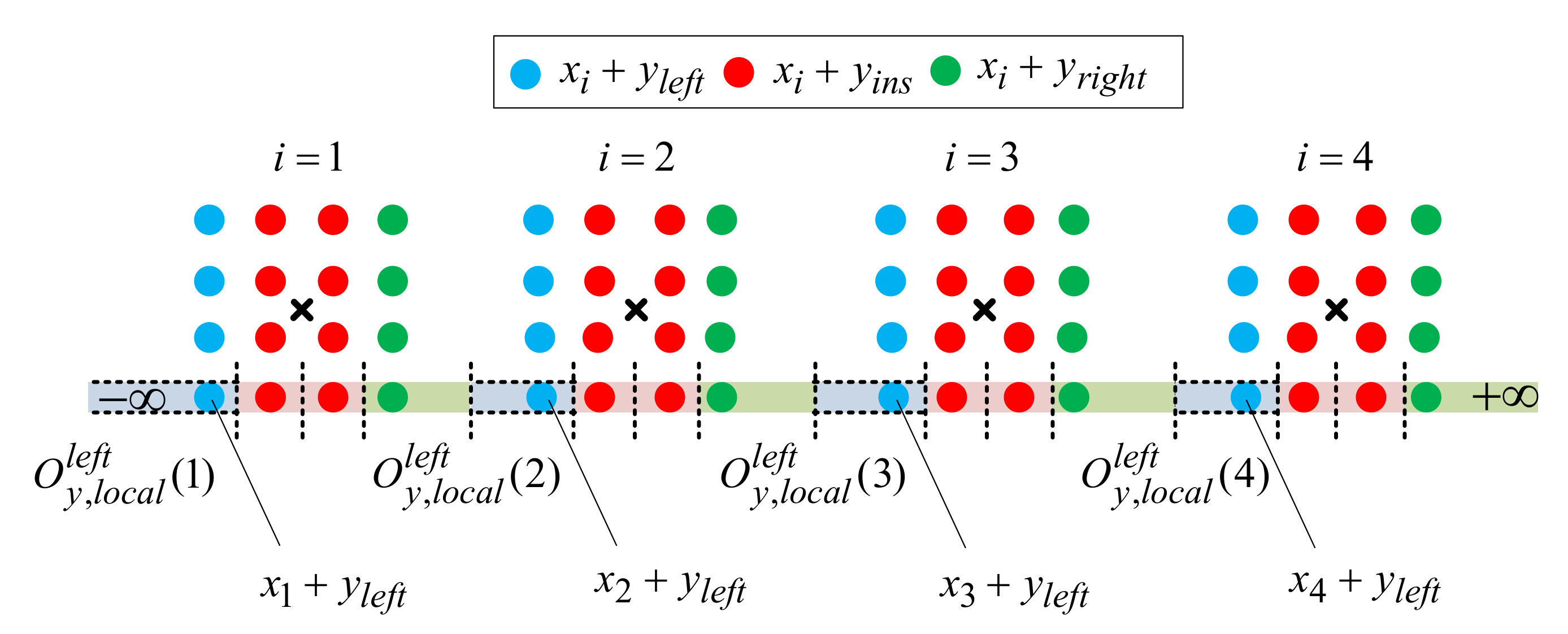
4.2. Second Layer Decoding

In this subsection, we derive SER and BER for the second non-orthogonal layer. According to the SIC, the decoding of the second layer is performed after decoding, regeneration, and cancellation of the first layer. If it is cancelled perfectly (without error), the updated received symbol is the superposition of the power weighted Q₂-QAM and noise realization. In this case, the probability of the error decoding is simply obtained in a similar way to (8), considering the symbol energy $p_2$, and given by

$$\rho (\overline{y}|correctx)=2\left(1-\frac{1}{\sqrt{Q_2}}\right)erfc\left(\sqrt{\frac{p_2}{M_2{N}_0}}\right)-\left(1-\frac{2}{\sqrt{Q_2}}+\frac{1}{Q_2}\right)erf{c}^2\left(\sqrt{\frac{p_2}{M_2{N}_0}}\right).$$

However, the error cancelling of x causes additional corruption of the second layer and increases the probability of its error decoding. In general, the probability of error decoding in the second non-orthogonal layer is obtained by

$$\rho \left(\overline{y}\right)=1-\rho ({\Re }_s\in O_y)\rho ({\Im }_s\in O_y),$$

where $\rho ({\Re }_s\in O_y)$ and $\rho ({\Im }_s\in O_y)$ are the probabilities that the real and imaginary components of the received symbol s fall into the decoding area of y. Note that $\rho ({\Re }_s\in O_y)$ and $\rho ({\Im }_s\in O_y)$ are identical and can be obtained by the same expression. Thus, we can modify the equation for $\rho \left(\overline{y}\right)$ as

$$\rho \left(\overline{y}\right)=1-\rho {({\Re }_s\in O_y)}^2.$$

(25)

Now, it is enough to derive the expression for the probability of the correct detection in the real region, and further, we focus only on it. The overall decoding area $O_y$ for each y is divided into several local areas. Let us look at the PD-NOMA constellation that is shown in Figure 1. The symbol y is decoded correctly when s falls in one of the sixteen (Q₁ = 16) areas near $\sqrt{p_1}x+\sqrt{p_2}y,\forall x\in A_1$. In general, the number of the detecting sections in the real region is $\sqrt{Q_1}$, and we obtain $\rho ({\Re }_s\in O_y)$ as follows

$$\rho ({\Re }_s\in O_y)={\displaystyle \sum _{i=1}^{\sqrt{Q_1}}\rho (x_i+y)\rho ({\Re }_{x_i+y}\in O_y)},$$

where $\rho (x_i+y)$ is the occurrence probability of the combination $x_i+y$ in the received symbol, and $\rho ({\Re }_{x_i+y}\in O_y)$ is the probability that the real component of the received symbol falls into its own detecting area. The main problem is that $\rho ({\Re }_{x_i+y}\in O_y)$ are not identical for different y because the detection sections are different. For example, Figure 2 shows the upper part of the PD-NOMA constellation from Figure 1. It is observed that y symbols on the left side of $x_i$ (blue dots) have detection segment boundaries, which are different from the symbols on the right side (green dots) as well as from the inside symbols (red dots). Thus, we divide $x_i+y$ by geometric position into three types ($x_i+y_{left},$ $x_i+y_{ins},$ $x_i+y_{right}$) with their detection areas $(O_y^{left},O_y^{ins},O_y^{right})$ and transform the equation for $\rho ({\Re }_s\in O_y)$ into

$$\rho ({\Re }_s\in O_y)={\displaystyle \sum _{i=1}^{\sqrt{Q_1}}\rho (x_i+y_{left})\rho ({\Re }_{x_i+y}{}_{{}_{left}}\in O_y^{left})}+{\displaystyle \sum _{i=1}^{\sqrt{Q_1}}\rho (x_i+y_{ins})\rho ({\Re }_{x_i+y}{}_{{}_{ins}}\in O_y^{ins})}+{\displaystyle \sum _{i=1}^{\sqrt{Q_1}}\rho (x_i+y_{right})\rho ({\Re }_{x_i+y}{}_{{}_{right}}\in O_y^{right})}$$

The occurrence probabilities for each type are $\rho (x_i+y_{left})=1/\sqrt{Q_2}$, $\rho (x_i+y_{right})=1/\sqrt{Q_2}$, $\rho (x_i+y_{ins})=1-2/\sqrt{Q_2}$, and by substituting them to the top equation, we obtain

$$\rho ({\Re }_s\in O_y)=\frac{1}{\sqrt{Q_2}}{\displaystyle \sum _{i=1}^{\sqrt{Q_1}}\rho ({\Re }_{x_i+y}{}_{{}_{left}}\in O_y^{left})}+\left(1-\frac{2}{\sqrt{Q_2}}\right){\displaystyle \sum _{i=1}^{\sqrt{Q_1}}\rho ({\Re }_{x_i+y}{}_{{}_{ins}}\in O_y^{ins})}+\frac{1}{\sqrt{Q_2}}{\displaystyle \sum _{i=1}^{\sqrt{Q_1}}\rho ({\Re }_{x_i+y}{}_{{}_{right}}\in O_y^{right})}$$

(26)

Now, we need obtain the probabilities for the symbol of each type falling into its own detection area. Firstly, let us focus on $x_i+y_{left}$ and derive the expression for $\rho ({\Re }_{x_i+y}{}_{{}_{left}}\in O_y^{left})$. We start with discussing the example given in Figure 2. The symbol $x_1+y_{left}$ is decoded correctly when ${\Re }_{x_1+y_{left}}\in O_{y,local}^{left}(m)\forall m\in \{1,2,3,4\}$, marked by the blue color. It is important that in the real domain, $O_{y,local}^{left}(1)$ is limited only on the right side by the neighboring inside symbol, and $O_{y,local}^{left}\left(2\right)$, $O_{y,local}^{left}\left(3\right)$, $O_{y,local}^{left}\left(4\right)$ are limited on both sides. Hence, the complete detection area $O_y^{left}$ is a compound of all local areas $O_y^{left}=\underset{m=1}{\stackrel{4}{\cup }}{O}_{y,local}^{left}(m)$. This conclusion is fair for $x_i+y_{left}\forall i\in 1\dots \sqrt{Q_1}$.

In a general case, for Q₁-QAM, we have $O_y^{left}=\underset{m=1}{\stackrel{4}{\cup }}{O}_{y,local}^{left}(m)$ and obtain $\rho ({\Re }_{x_i+y_{left}}\in O_y^{left})$ by using Gauss error function according to

$$\begin{array}{l}\rho ({\Re }_{x_i+y_{left}}\in O_y^{left})=1-\frac{1}{2}{\displaystyle \sum _{m=1}^{\sqrt{Q_1}-1}\left[erf\left(\frac{\left(\sqrt{Q_1}-i-m+\frac{1}{2}\right)D_1+\left(0.5\sqrt{Q_2}-\frac{1}{2}\right)D_2}{\sqrt{N_0}}\right)\right.}\left.-erf\left(\frac{\left(\sqrt{Q_1}-i-m+1\right)D_1+\frac{1}{2}{D}_2}{\sqrt{N_0}}\right)\right]\\ -\frac{1}{2}erf\left(\frac{\left(1-i\right)D_1+\frac{1}{2}{D}_2}{\sqrt{N_0}}\right)\end{array}$$

To simplify the further expressions, we denote a set of the following variables

$$\begin{array}{l}{V}_{i,m}^{\pm }=erf\left[\frac{\left(\sqrt{Q_1}-i-m+1\right)D_1\pm 0.5D_2}{\sqrt{N_0}}\right]\\ C_{i,m}^{\pm }=erf\left[\frac{\left(\sqrt{Q_1}-i-m+0.5\right)D_1\pm \left(0.5\sqrt{Q_2}-0.5\right)D_2}{\sqrt{N_0}}\right]\\ B_i^{\pm }=erf\left[\frac{\left(1-i\right)D_1\pm 0.5D_2}{\sqrt{N_0}}\right]\end{array}$$

(27)

and by using (27), transform the equation for $\rho ({\Re }_{x_i+y_{left}}\in O_y^{left})$ according to

$$\rho ({\Re }_{x_i+y_{left}}\in O_y^{left})=1-\frac{1}{2}\left[{\displaystyle \sum _{m=1}^{\sqrt{Q_1}-1}\left(C_{i,m}^{+}-V_{i,m}^{+}\right)}-B_i^{+}\right],$$

(28)

The same procedure can be applied to obtaining $\rho ({\Re }_{x_i+y_{left}}\in O_y^{right})$, considering that $O_y^{right}$ has the same bounds as $O_y^{left}$, which are symmetric with respect to the zero. Thus, we derive the equation by using the variables in (27) according to

$$\rho ({\Re }_{x_i+y_{right}}\in O_y^{right})=\frac{1}{2}\left[{\displaystyle \sum _{m=1}^{\sqrt{Q_1}-1}\left(C_{i,m}^{-}-V_{i,m}^{-}\right)}-B_i^{-}\right],$$

(29)

Finally, $\rho ({\Re }_{x_i+y_{ins}}\in O_y^{ins})$ is obtained the most easily because each i-th combination has the uniform bounds of $O_y^{ins}$, which are limited on both sides. By utilizing this statement, we have

$$\rho ({\Re }_{x_i+y_{ins}}\in O_y^{ins})={\displaystyle \sum _{m=1}^{\sqrt{Q_1}}\left[erf\left(\frac{(2-m)D_1+0.5D_2}{\sqrt{N_0}}\right)-erf\left(\frac{(2-m)D_1-0.5D_2}{\sqrt{N_0}}\right)\right]},$$

(30)

We denote a new variable $G_n^{\pm }$, given by

$$G_m^{\pm }=erf\left[\frac{(2-m)D_1\pm 0.5D_2}{\sqrt{N_0}}\right],$$

(31)

and (30) can be expressed as

$$\rho ({\Re }_{x_i+y_{ins}}\in O_y^{ins})=\frac{1}{2}{\displaystyle \sum _{m=1}^{\sqrt{Q_1}}(G_m^{+}-G_m^{-})}.$$

(32)

Next, $\rho ({\Re }_s\in O_y)$ is obtained by substituting (28), (29), and (30) into (26) as follows

$$\rho ({\Re }_s\in O_y)=\frac{1}{\sqrt{Q_2}}+\left(\frac{1}{2}-\frac{1}{\sqrt{Q_2}}\right)\times {\displaystyle \sum _{m=1}^{\sqrt{Q_1}}\left(G_m^{+}-G_m^{-}\right)}-\frac{1}{2\sqrt{Q_1{Q}_2}}\times {\displaystyle \sum _{i=1}^{\sqrt{Q_1}}\left[{\displaystyle \sum _{m=1}^{\sqrt{Q_1}-1}\left(V_{i,m}^{-}-V_{i,m}^{+}+C_{i,m}^{+}-C_{i,m}^{-}\right)}-B_i^{+}+B_i^{-}\right]}.$$

(33)

Based on the identical probability for the real and imaginary components, we directly obtain the symbol error rate in the second non-orthogonal layer by placing (33) to (25) and simplifying the equation according to

$$\rho (\overline{y})=1-\left\{\frac{1}{\sqrt{Q_2}}\right.+\left(\frac{1}{2}-\frac{1}{\sqrt{Q_2}}\right)\times {\displaystyle \sum _{m=1}^{\sqrt{Q_1}}\left(G_m^{+}-G_m^{-}\right)}{\left.-\frac{1}{2\sqrt{Q_1{Q}_2}}\times {\displaystyle \sum _{i=1}^{\sqrt{Q_1}}\left[{\displaystyle \sum _{m=1}^{\sqrt{Q_1}-1}\left(V_{i,m}^{-}-V_{i,m}^{+}+C_{i,m}^{+}-C_{i,m}^{-}\right)}-B_i^{+}+B_i^{-}\right]}\right\}}^2.$$

(34)

Finally, BER in the second non-orthogonal layer is obtained similarly to (24) by the approximation of $\rho \left(\overline{y}\right)$ on $lo{g}_2\left(Q_2\right)$ in the following way

$${\rho }_b(\overline{y})\approx \frac{\rho \left(\overline{y}\right)}{lo{g}_2\left(Q_2\right)}.$$

(35)

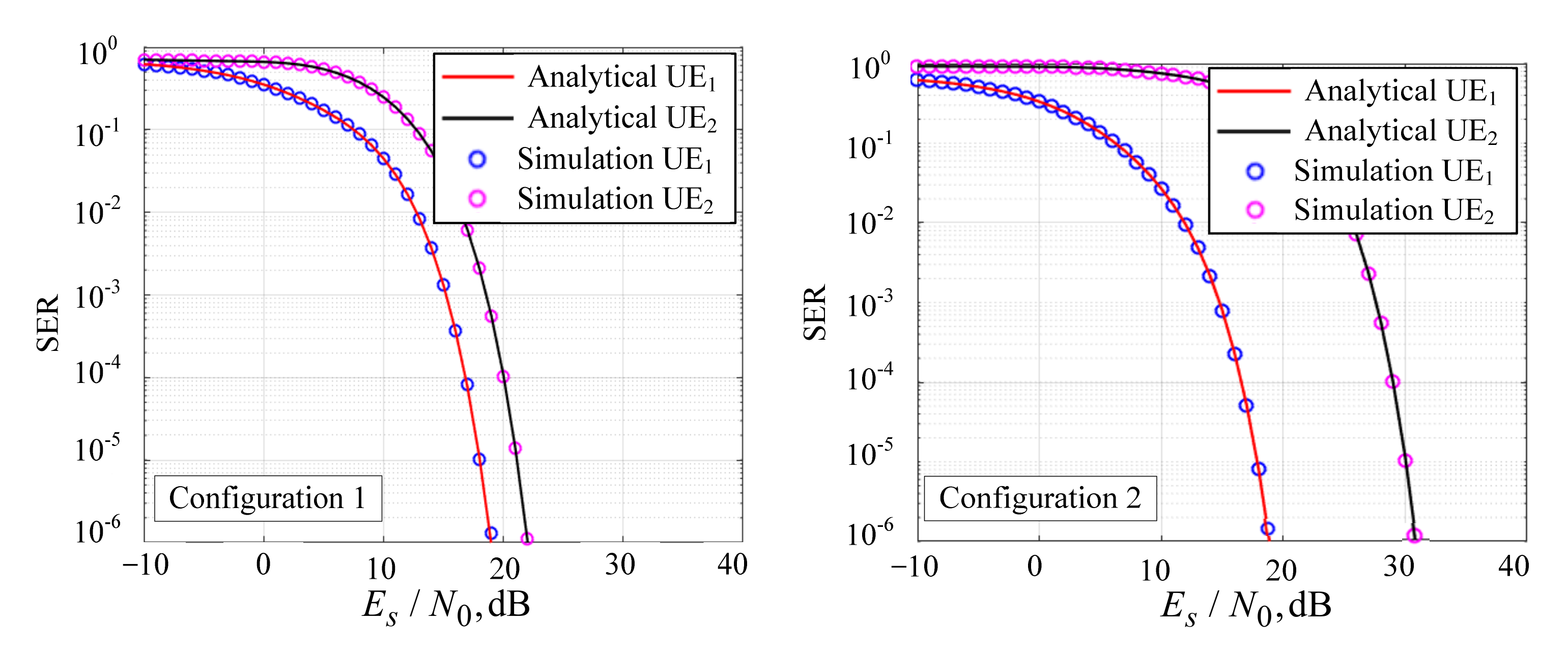
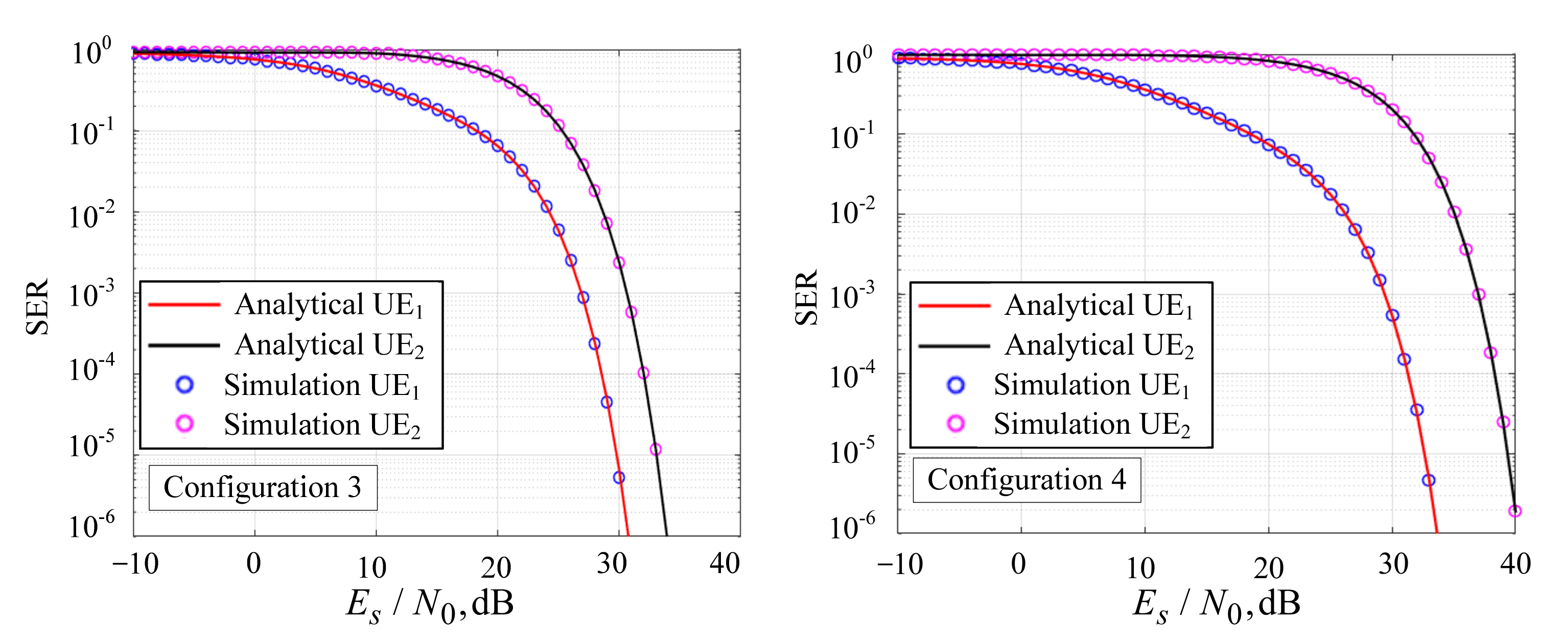
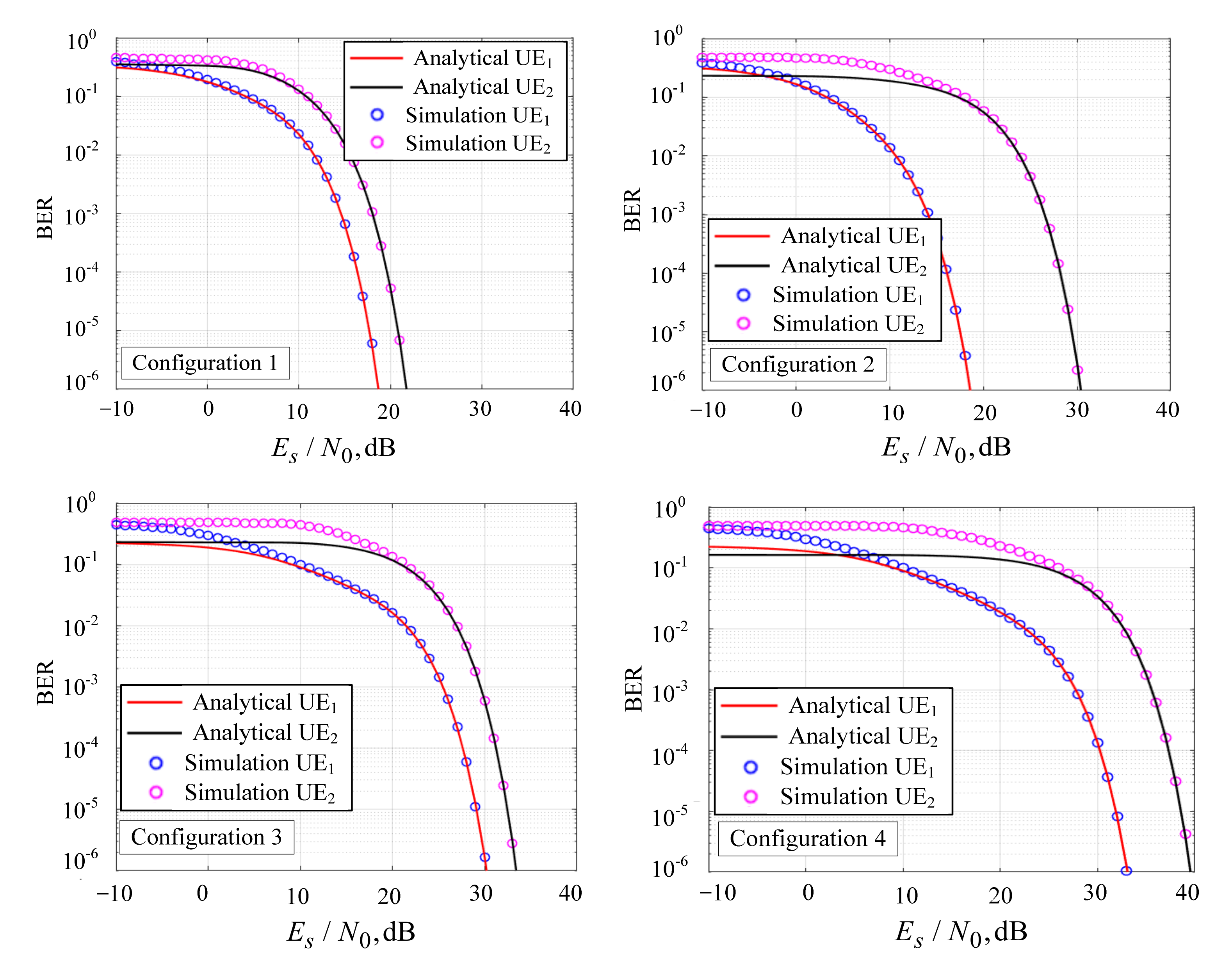
5. BER and SER Simulation

We use the Monte Carlo simulation carried out in MATLAB to validate the theoretical results from the previous section. This is often used to model the probability of different outcomes in a process that cannot easily be predicted due to the intervention of random variables. In communication, the MC simulation is used to estimate the probability of signal decoding under the noise by performing a large number of simulations and averaging the results.

The SER and BER are obtained from the simulation model and compared with the analytical values calculated by (23, 34) and (24, 35). In Figure 3, the simulation scheme of the two-user downlink PD-NOMA via the AWGN channel is presented. We use a signal construction based on square QAM with Gray coding without any error correction techniques. In the simulation scheme, $b_x$,$b_y$ are the vectors that contain transmission bits, and x, y are the modulation symbols of UE₁ and UE₂. In the following simulations, we assume that the complex noise realizations of both users are $w_1,w_2~CN(0,N_0)$ and they are controlled by $E_s/N_0$ in the range from −10 to 40 dB with a 1 dB step.

In general, the number of possible PD-NOMA multiplexing configurations is not limited, so any of them can be chosen for simulation. As an example, we have selected the four most illustrative scenarios of a PD-NOMA layer configuration with typical wireless network modulation orders and power weights considering the most possible exploitation scenarios. They are shown in

Table 1. PD-NOMA configurations.

No.	First Layer (UE1)		Second Layer (UE2)
	p1	Q1	p2	Q2
1	0.85	4	0.15	4
2	0.9	4	0.1	16
3	0.95	16	0.05	16
4	0.95	16	0.05	64

and include various combinations of power weights and QAM orders.

Figure 4 shows the comparison of the theoretical and simulated SER with $E_s/N_0$ for each scenario. The analytical SERs are submitted by solid lines, and the simulated SERs are plotted by markers. It is observed that the analytical SERs of both users match the simulated SERs perfectly for all the multiplexing configurations in the full range of $E_s/N_0$. Due to the comparison result, we validated the (23) and (34) expressions, which were obtained in the previous section. We can also conclude that the presented expressions can be perfectly used for the SER calculation in both user QAM signals multiplexed by PD-NOMA.

The comparison of the theoretical and simulated BERs against $E_s/N_0$ is presented in Figure 5. We observe that the analytical BER expressions of both users in the PD-NOMA system match the simulation results in the low BER region, which perfectly validates (24) and (35). In the high BER region, we remark that the accuracy of the analytical result is decreased due to the approximation inexactness. The validation result demonstrates that the presented expressions cannot be applied to obtain accurate BER values in the high BER region due to the used approximation. This issue requires further investigation and will be solved in the following works.

6. Conclusions

In this paper, BER and SER analytical expressions for two-user square QAM signals multiplexed by PD-NOMA and transmitted through the AWGN channel were proposed. The calculation requires the known PD-NOMA configuration, including QAM order and power weights of each user signal.

The validation of the expressions using simulation is provided in Section 5. The SER and BER values obtained from the simulation are compared with the calculated analytical values. In order to make a reliable comparison, we have used four various PD-NOMA configurations. The following conclusions can be made on the basis of the obtained results, and their analysis:

(1) The comparison result has shown that the SER analytical result perfectly coincides with the simulation result, which confirms the credibility of the obtained expressions. Therefore, the SER values for the PD-NOMA system described above can be exactly calculated by proposed expressions without difficulty simulation.

(2) In turn, the BER analytical result matches with the simulation result only in the low BER region (<10⁻²). Thus, the analytical BER expressions can be used for a rough estimate in the high BER region and for accurate calculation in the low BER region. The issue of error estimation in the high BER region will be solved in the following works.

The goal of subsequent work is the further research of an error rate performance of PD-NOMA group channel in different multiplexing configurations by using received analytical expressions. In the future, we will design a table with adaptive joint modulation and coding schemes (MCS) for adaptive configuration selection based on the MCSs from the 5G NR standard. This table will be used in optimal group signal formation, scheduling, estimation of an achievable practice performance of PD-NOMA, etc.

References

- Saito, Y.; Benjebbour, A.; Kishiyama, Y.; Nakamura, T. System-level performance evaluation of downlink non-orthogonal multiple access (NOMA). In Proceedings of the 2013 IEEE 24th International Symposium on Personal, Indoor and Mobile Radio Communications (PIMRC), London, UK, 8–11 September 2013; pp. 611–615. [Google Scholar]
- Saito, Y. Non-orthogonal multiple access (NOMA) for cellular future radio access. In Proceedings of the 2013 IEEE 77th Vehicular Technology Conference (VTC Spring), Dresden, Germany, 2–5 June 2013. [Google Scholar]
- Ding, Z.; Lei, X.; Karagiannidis, G.K.; Schober, R.; Yuan, J.; Bhargava, V.K. A survey on non-orthogonal multiple access for 5G networks: Research challenges and future trends. IEEE J. Sel. Areas Commun. 2017, 35, 2181–2195. [Google Scholar] [CrossRef] [Green Version]
- Benjebbour, A.; Saito, K.; Li, A.; Kishiyama, Y.; Nakamura, T. Non-orthogonal multiple access (NOMA): Concept, performance evaluation and experimental trials. In Proceedings of the 2015 International Conference on Wireless Networks and Mobile Communications (WINCOM), Marrakech, Morocco, 20–23 October 2015. [Google Scholar]
- Shin, W.; Vaezi, M.; Lee, B.; Love, D.J.; Lee, J.; Poor, H.V. Non-orthogonal multiple access in multi-cell networks: Theory, performance, and practical challenges. IEEE Commun. Mag. 2017, 55, 176–183. [Google Scholar] [CrossRef] [Green Version]
- Islam, S.R.; Avazov, N.; Dobre, O.A.; Kwak, K.S. Power-domain non-orthogonal multiple access (NOMA) in 5G systems: Potentials and challenges. IEEE Commun. Surv. Tutor. 2016, 19, 721–742. [Google Scholar] [CrossRef] [Green Version]
- Liu, C.H.; Liang, D.C. Heterogeneous networks with power-domain NOMA: Coverage, throughput, and power allocation analysis. IEEE Trans. Wirel. Commun. 2018, 17, 3524–3539. [Google Scholar] [CrossRef] [Green Version]
- Higuchi, K.; Benjebbour, A. Non-orthogonal multiple access (NOMA) with successive interference cancellation for future radio access. IEICE Trans. Commun. 2015, 98, 403–414. [Google Scholar] [CrossRef] [Green Version]
- Cui, J.; Liu, Y.; Ding, Z.; Fan, P.; Nallanathan, A. Optimal user scheduling and power allocation for millimeter wave NOMA systems. IEEE Trans. Wirel. Commun. 2017, 17, 1502–1517. [Google Scholar] [CrossRef] [Green Version]
- Chen, X.; Benjebbour, A.; Li, A.; Harada, A. Multi-user proportional fair scheduling for uplink non-orthogonal multiple access (NOMA). In Proceedings of the 2014 IEEE 79th Vehicular Technology Conference (VTC Spring), Seoul, Korea, 18–21 May 2014. [Google Scholar]
- Rai, R.; Zhu, H.; Wang, J. Resource scheduling in non-orthogonal multiple access (NOMA) based cloud-RAN systems. In Proceedings of the 2017 IEEE 8th Annual Ubiquitous Computing, Electronics and Mobile Communication Conference (UEMCON), New York, NY, USA, 19–21 October 2017; pp. 418–422. [Google Scholar]
- Uddin, M.F. Energy efficiency maximization by joint transmission scheduling and resource allocation in downlink NOMA cellular networks. Comput. Netw. 2019, 159, 37–50. [Google Scholar] [CrossRef]
- Fang, F.; Zhang, H.; Cheng, J.; Roy, S.; Leung, V.C. Joint user scheduling and power allocation optimization for energy-efficient NOMA systems with imperfect CSI. IEEE J. Sel. Areas Commun. 2017, 35, 2874–2885. [Google Scholar] [CrossRef]
- Kryukov, Y.V.; Brovkin, A.A.; Pokamestov, D.A.; Kvashnina, A.S. A simple proportional fair scheduling for downlink power domain non-orthogonal multiple access systems. Journal of Physics: Conference Series. IOP Publ. 2020, 1679, 032055. [Google Scholar]
- Kryukov, Y.V.; Pokamestov, D.A.; Brovkin, A.A.; Rogozhnikov, E.V. Power and Frequency Scheduling Using Equal Throughput Strategy in PD-NOMA Systems. In Computer Science Online Conference; Springer: Cham, Switzerland, 2020; pp. 584–595. [Google Scholar]
- Zeng, M.; Yadav, A.; Dobre, O.A.; Tsiropoulos, G.I.; Poor, H.V. Capacity comparison between MIMO-NOMA and MIMO-OMA with multiple users in a cluster. IEEE J. Sel. Areas Commun. 2017, 35, 2413–2424. [Google Scholar] [CrossRef]
- Wei, Z.; Yang, L.; Ng, D.W.K.; Yuan, J.; Hanzo, L. On the performance gain of NOMA over OMA in uplink communication systems. IEEE Trans. Commun. 2019, 68, 536–568. [Google Scholar] [CrossRef] [Green Version]
- Wyner, A. Recent results in the Shannon theory. IEEE Trans. Inf. Theory 1974, 20, 2–10. [Google Scholar] [CrossRef]
- Meghdadi, V. BER calculation. In Wireless Communications; 2008; Available online: https://www.unilim.fr/pages_perso/vahid.meghdadi-neyshabouri/notes/ber_awgn.pdf (accessed on 1 October 2021).
- Kara, F.; Kaya, H. BER performances of downlink and uplink NOMA in the presence of SIC errors over fading channels. IET Commun. 2018, 12, 1834–1844. [Google Scholar] [CrossRef]
- Assaf, T.; Al-Dweik, A.; Moursi, M.E.; Zeineldin, H. Exact BER performance analysis for downlink NOMA systems over Nakagami-m fading channels. IEEE Access 2019, 7, 134539–134555. [Google Scholar] [CrossRef]
- Wang, X.; Labeau, F.; Mei, L. Closed-form BER expressions of QPSK constellation for uplink non-orthogonal multiple access (NOMA). IEEE Commun. Lett. 2017, 21, 2242–2245. [Google Scholar] [CrossRef]
- Han, W.; Wang, Y.; Tang, D.; Hou, R.; Ma, X. Study of the Symbol Error Rate/Bit Error Rate in Non-orthogonal Multiple Access (NOMA) Systems. In Proceedings of the 2018 IEEE/CIC International Conference on Communications in China (ICCC Workshops), Beijing, China, 16–18 August 2018; pp. 101–106. [Google Scholar]
- Huang, H.; Wang, J.; Wang, J.; Yang, J.; Xiong, J.; Gui, G. Symbol error rate performance analysis of non-orthogonal multiple access for visible light communications. China Commun. 2017, 14, 153–161. [Google Scholar] [CrossRef]
- Almohimmah, E.M.; Alresheedi, M.T. Error analysis of NOMAbased VLC systems with higher order modulation schemes. IEEE Access 2020, 8, 2792–2803. [Google Scholar] [CrossRef]
- Lee, E.A.; Messerschmitt, D.G. Digital Communication; Springer Science & Business Media: Berlin/Heidelberg, Germany, 2012; Available online: https://www.amazon.com/Digital-Communication-John-R-Barry-dp-1461349753/dp/1461349753/ref=mt_other?_encoding=UTF8&me=&qid= (accessed on 1 October 2021).