1. Introduction
The energy sector is one of the essential factors in modern society, and thus the required amount of energy between supply and demand should be balanced. As a result, energy forecasting plays a vital role in helping energy manufacturers. Additionally, it is helpful in the improvement of energy management systems, planning, and operation [
1,
2]. Energy forecasting can be categorized into three groups in term forecasting ranges: one hour–one week, one month–one year, and more than one year, correspondingly [
3]. In this paper, short-term hourly energy forecasting is conducted because it is an effectively helpful tool for reducing energy generating and operating costs, ensure power system security, and perform short-term scheduling functions.
According to the benefits mentioned above, many researchers proposed numerous scientific models to achieve better performance on energy forecasting. Generally, forecasting models can be regarded as traditional statistical models and artificial intelligence (AI)-based models. Warren McCulloch and Walter Pitts firstly introduced the foundations of the AI network in 1943 [
4]. Since then, AI-based machine learning (ML) models have been widely used in medicine, business, communications, and industrial process control as nonlinear time series problems can be solved. Nevertheless, deep learning (DL) models were established to handle the weakness of ML models. For instance, the training process of ML models could cost a longer computational time during the backpropagation process if there were multiple layers in the network. Moreover, there is no interconnection between each layer in the traditional ML that causes the lack of information for time series data. Multilayer perceptron (MLP) [
5], convolutional neural network (CNN) [
6], and long short-term memory (LSTM) [
7] are proposed to solve ML weakness for time series forecasting. Consequently, this article was applied these DL models to implement and improve forecasting accuracy based on energy time series data. Additionally, time series forecasting effectively supports demand management in the electric industry.
Naturally, complex seasonality patterns are exhibited in such time series data. For example, seasonal, calendar, and weather effects significantly influence energy consumption [
8]. Firstly, seasonal effects involve four seasons: spring, summer, fall, and winter in Jeju. Secondly, calendar effects consist of day type, month, public holiday, and national holiday. Finally, weather effects are typically associated with meteorological circumstances such as temperature, cloudy, and humidity [
9]. As a result, this study primarily considers the weather information, including temperature, dew point, humidity, wind speed, solar radiation, and other factors for better understanding the non-linear relationship between load patterns and influential variables that can enhance energy forecasting performance.
This research mainly uses the ensemble model of the latest advanced DL models for time series energy forecasting. Hence, four advanced DL models such as MLP, CNN, LSTM, and hybrid CNN-LSTM are applied and implemented for forecasting. These models can effectively handle the time series data by memorizing all sequences during the training process. This work compares the proposed ensemble model with the standard baseline forecasting models by preserving the feature engineering. Three error metrics, including mean square error (MSE), mean absolute error (MAE), and mean absolute percentage error (MAPE), are evaluated to make a performance comparison among all models.
1.1. Related Work
Lim and Zohren surveyed on developing DL architectures and hybrid DL models combining well-studied statistical models with neural network components for time series forecasting [
10]. Furthermore, Langkvist et al. reviewed the development of DL and unsupervised feature learning for time series problems by suggesting ML and DL algorithms [
11]. Compared to ML models, the experiment of DL algorithms provides the capability to cope with nonlinear relationships, model complexity, and computational efficiency. The clarification review of DL algorithms such as deep neural network (DNN), unsupervised learning, and reinforcement learning from prior works was conducted by Schmidhuber [
12]. In the article of Hosein, the better results of DNN were compared with those of ML algorithms using periodic smart meter energy for short-term load forecasting [
13]. The application of the multilayered DNN training along with different activation functions sigmoid, rectifier linear unit (ReLU), and exponential linear unit (ELU) to the Iberian electric market forecasting were investigated in work by Hossen et al. [
14].
In the study of Cai et al., DL models including the recurrent neural network (RNN) and CNN models were compared with an autoregressive integrated moving average with exogenous inputs (ARIMAX) regarding the forecasting accuracy, computational efficiency, generalizability, and robustness [
15]. Moreover, the effectiveness of the CNN algorithm was investigated by comparing experimental results to other ML and DL algorithms for energy load forecasting [
16]. The LSTM prediction models with various configurations were constructed using France metropolitan’s electricity consumption data for short- and medium-term load forecasting. They compared the relevant performance to ML models [
17]. Besides, LSTM multi-input, multioutput models considering long-term historical dependencies for the cluster analysis of load trend were trained and opposed the performance to ML models [
18]. Kong et al. also implemented the LSTM model on residential smart meter data, which outperformed backpropagation neural network (BPNN) in the task of short-term load forecasting [
19]. These prior works provided reasonable and good forecasting results using the latest popular DL models.
On the other hand, considering the benefits and drawbacks of ML and DL algorithms, various studies were employed either a hybrid method or an ensemble method to execute more reliable and accurate forecasting outcomes [
20,
21,
22,
23]. The incorporation of an artificial neural network (ANN), a BPNN, a generalized regression neural network (GRNN), an Elman neural network, and a genetic algorithm optimized backpropagation neural network (GABPNN) was proposed for half-hourly electrical power prediction by Xiao et al. [
24]. The hybrid algorithm, so-called SDEMD-LSTM, combining similar days (SD) selection, empirical mode decomposition (EMD), and LSTM networks, was conducted by Zheng et al. [
25]. Their study evaluated the similarity between forecast and historical days by using the extreme gradient boosting-based weighted k-means algorithm. Furthermore, the ensemble method, including the EMD algorithm and the deep belief network (DBN) trained with two restricted Boltzmann machines (RBMs), were performed on electricity load demand [
26]. This effectiveness experiment of the proposed EMD-based DBN model outperformed nine other forecasting methods in comparing simulated results. In the article by Zhang and Wang, another decomposition-ensemble method composed of SSA, SVM, ARIMA, and CS algorithms, was integrated for load forecasting. Their empirical outcomes ensured the importance of an ensemble model based on data input structure [
27]. Regarding these prior works, the ensemble method combining two or more forecasting models could be essential to improve the forecasting performance in many areas, such as forecasting of the daily average number of COVID-19 patients, bitcoin price forecasting, household load forecasting, and typhoon formation forecasting [
28,
29,
30,
31].
1.2. Contribution
For the first time, this work handles time-series problems using the three latest advanced DL models and the hybrid CNN-LSTM model while considering the tuning parameters based on collected data. The ensemble combination of these four advanced DL models is a novelty proposed to improve energy forecasting performance. For better training, all DL models also consider weather features that affect energy consumption.
1.3. Paper Organization
This paper is organized using the following sections. The methodology, including DL architectures and the main framework of our proposed model, are described in
Section 2. The results are then discussed and compared in
Section 3. The conclusion of the complete work is written in the last section.
2. Methodology
In this section, deep neural networks-based models such as MLP, CNN, LSTM, hybrid CNN-LSTM, and our proposed ensemble model are described with a detailed explanation of their architectures and parameters applied in this research.
2.1. Multilayer Perceptron (MLP)
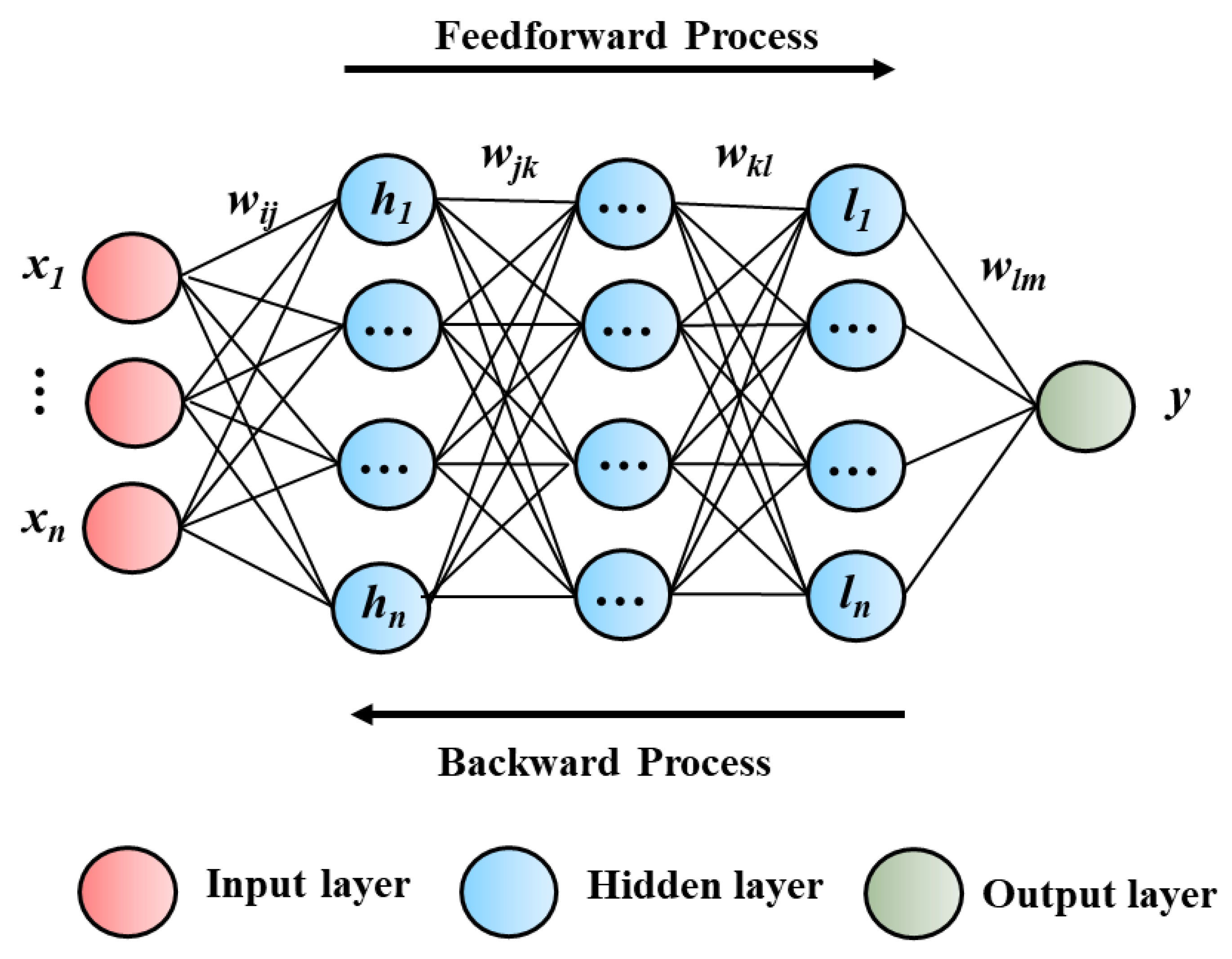
Like an ordinary neural network, an MLP has an input, output, and hidden layer. However, it can have many layers in its training process. There are two training processes: feedforward propagation and backward propagation in the MLP network. In the former approach, neuron nodes for input features are multiplied with respective weights and biases to execute the corresponding output values passing through nonlinear activation functions of all invisible layers. The latter process adjusts the weights to minimize the loss using backpropagation gradient descent after estimating the target and calculating loss in the forward direction. The structure of the MLP network training process is shown in
Figure 1. The mathematical expression of the MLP is written as:
where,
= the predicted output at the
mth output layer,
= the output at the
l hidden layer,
= the weight between the
lth hidden layer and the
mth output layer,
= the weight at the
mth output layer,
f = activation function,
i = the input layer,
m = the output layer.
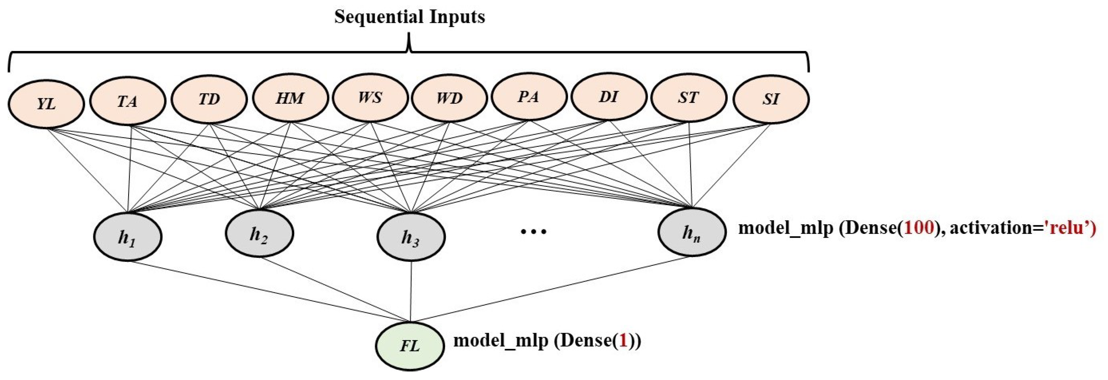
In this paper, MLP is firstly used as one of the DL models to execute our proposed ensemble DL model.
Figure 2 indicates our proposed MLP model with one input layer, one hidden layer, and one output layer. The formation of all inputs is used as sequential data. Thus, the MLP network has the input for each sample in terms of the number of time steps. Ten sequential training inputs are initially loaded into the MLP training model. Afterward, the model is fitted with 100 dense layers and a Rectified Linear Unit (ReLU) activation function. Finally, the model predicted results based on the test data at the last dense layer.
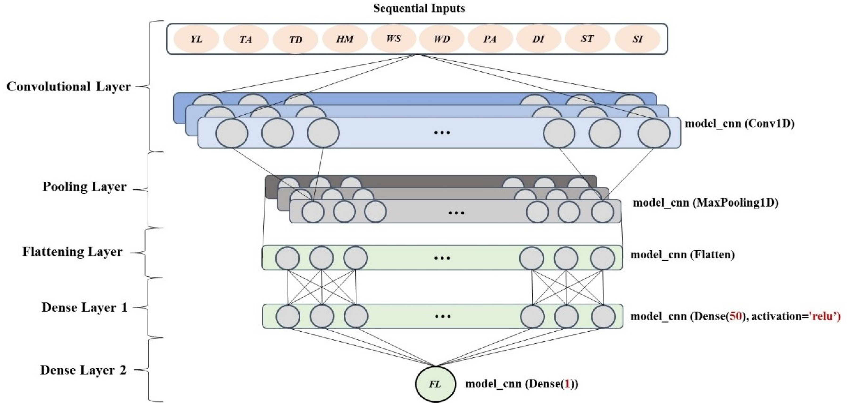
2.2. Convolutional Neural Network (CNN)
The second proposed DL model is CNN architecture which contains several layers, so-called multibuilding blocks. The detail of each layer in the CNN architecture is described in
Figure 3. Firstly, the sequential data are imported to a convolutional layer convolved as a one-dimensional structure with 64 filters, two kernel sizes, and the ReLU activation function to generate the output feature map. The next layer is a pooling layer which shrinks large-size feature maps to create smaller feature maps. The one-dimensional maximum (max) pooling with two pool sizes is applied in our case. After that, the data are converted into a one-dimensional array by a flattening layer. It is imported to the fully connected layer of the CNN model, having fifty dense layers and the ReLU activation function. Ultimately, the final layer executes the output on test prediction.
2.3. Long Short-Term Memory (LSTM)
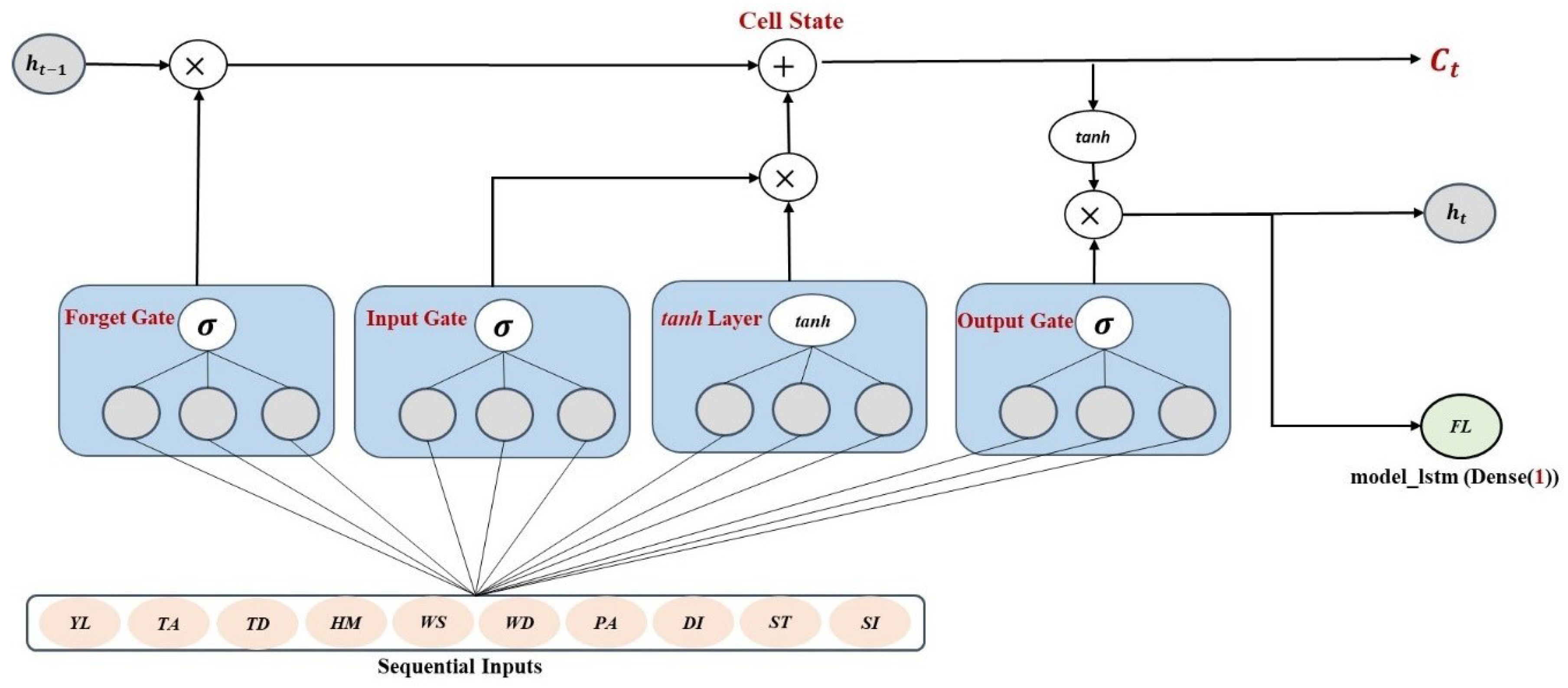
The third DL model is the LSTM network which consists of a set of recurrently connected subnets, known as memory blocks. Each memory block includes a memory cell, input gate, forget gate, and output gate. Unlike the traditional recurrent unit, which overwrites its content at each step, the LSTM unit can decide whether to keep the existing memory via the introduced gates. LSTM avoids the long-term dependency problem explicitly. There are four interacting layers in the LSTM architecture instead of having a single neural network layer in a recurrent neural network.
Figure 4 shows the structure of LSTM where each line carries an entire vector, from the output of one node to the inputs of the other.
Initially, the forget gate (sigmoid) layer takes an input that is needed to be kept and the previously hidden layer to give an output in the cell state. Afterward, an input gate (sigmoid) layer updates the input value, and then multiplies it with a tanh layer, creating a vector of new candidate values. The new cell state is then executed by combining the old state and a new candidate value. Next, an output gate (sigmoid) layer performs an output using the new cell state passing through the tanh layer. Finally, the desired result is filtered by multiplying the output layer and the tanh layer. In this study, LSTM is implemented with the ReLU activation function.
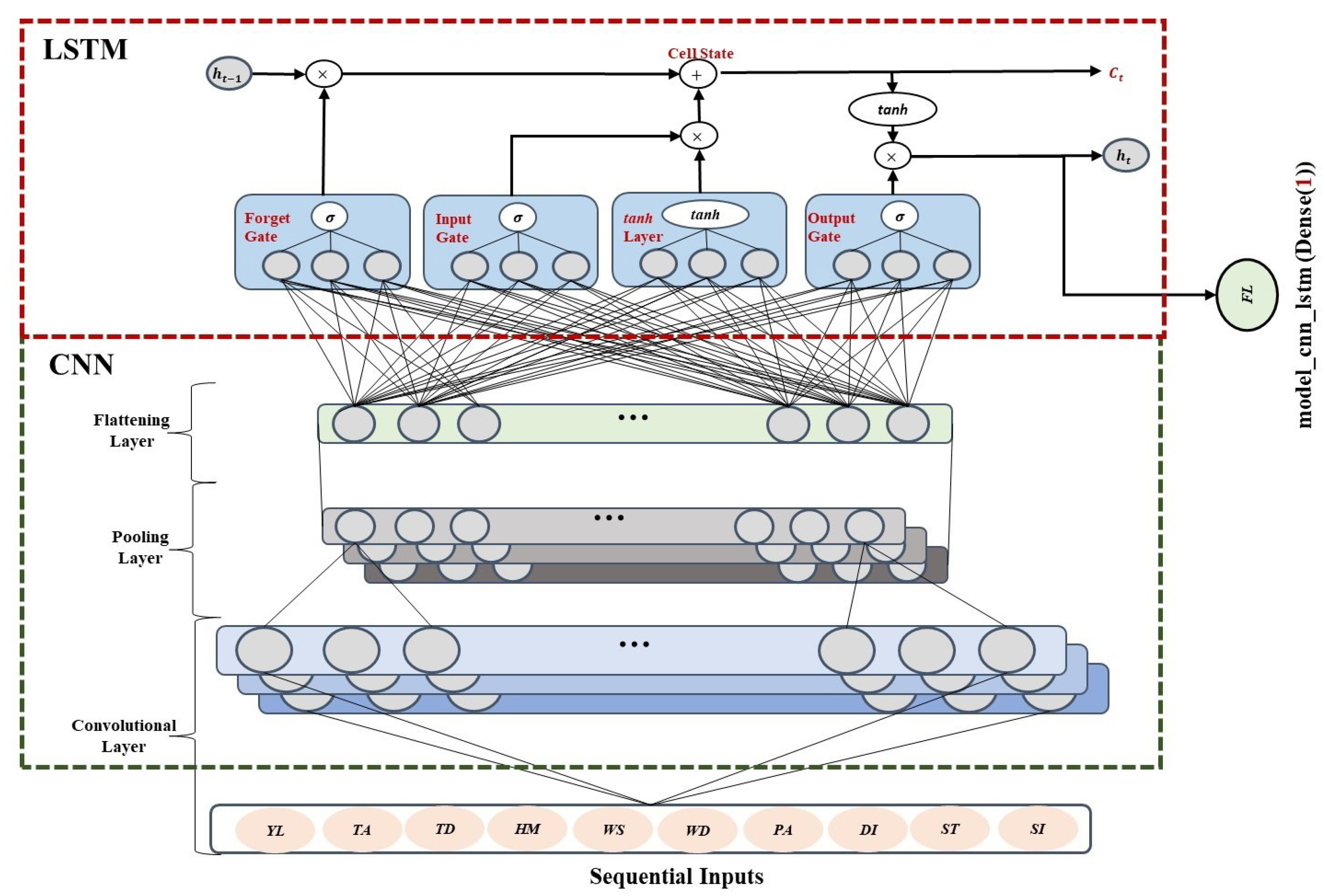
2.4. Hybrid CNN-LSTM
A hybrid CNN-LSTM model is our last DL ensemble method. Very long input sequences can be handled as blocks or subsequences as the hybrid model contains both CNN and LSTM models. In this case, our sequential data are divided into further subsequences for each sample to train the hybrid model. A hybrid structure of CNN and LSTM models is represented in
Figure 5. Primarily, the CNN model interprets each subsequence of sequential inputs. In this case, the CNN model is enveloped in Time Distributed wrapper layers of convolution, pooling, and flattening. Hereafter, the results are assembled by the LSTM layer before making a test prediction. The parameters of the hybrid model are adjusted in the same manner as stand-alone CNN and LSTM models.
2.5. Ensemble Deep Learning Model
2.5.1. Data Management
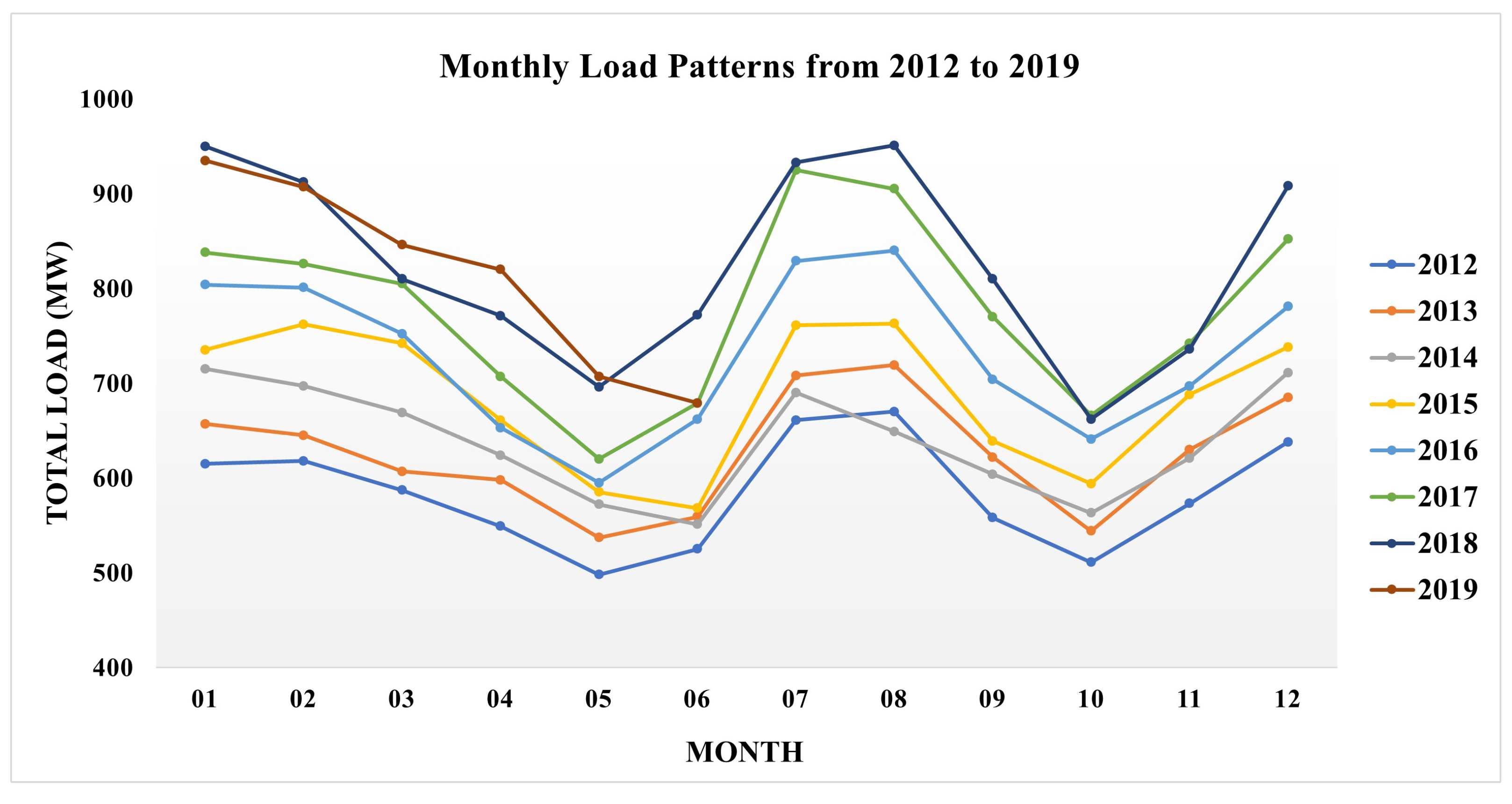
The hourly-based energy consumption data are gathered from four weather stations such as Jeju-si, Gosan, Seongson, and Seogwipo of Jeju Island. The total load data of the whole Jeju are recorded from 2012 to June 2019, as indicated in
Figure 6. It is obvious that energy consumption increases year by year due to the development of population and industries. Jeju has four seasons: spring from March to May, summer from June to August, fall from September to November, and winter from December to February. Generally, energy usage rises during summer when the peak load has occurred. Similarly, people consume higher electricity to keep warm in the winter season. During the spring and fall seasons of the specified years, the usage of energy varies approximately from 500 to 900 MW.
Each station also collects the weather information separately. Collected hourly-based weather features are average temperature (TA), dew point temperature (TD), humidity (HM), wind speed (WS), wind direction degree (WD), atmospheric pressure on the ground (PA), discomfort index (DI), sensible temperature (ST), and solar irradiation quantity (SI). Our earlier work has widely explained the correlation between total load consumption and weather features from each station [
20]. Some extra features are also added in this work, as demonstrated in
Table 1. The table shows that positive values mean a strong correlation between two features, while negative values indicate less correlation. Therefore, the most affecting factor on load is the PA feature from all stations, showing around 0.23. The WS feature is ranked second at Jeju-si and Gosan, whereas WD is for Seongsan and Seogwipo. The WD is another influential feature on load for all stations, except Gosan. The rest features are given as negative correlation so that the impact of external factors is meager.
In this work, our dataset was collected from four geographic parts of Jeju (including Jeju-si, Seongwipo, Gosan, and Seongson). Each region had its weather information containing nine features and the total load over the grid, and we used percentage-based division and aggregation approaches to reduce the dataset. The preprocessing method considered 50% of data from Jeju-si as it is a highly-populated area, and it matters the most. Similarly, we utilized 30% from Seogwipo, 10% from Gosan, and 10% from Seongsan. Therefore, ten sequential inputs, including load and nine weather features, are applied to train all DL models. The following expression is the vector of input features.
where,
= the forecasted load vector of input features,
= the yesterday load at time
t,
.
2.5.2. Set Up Parameters
Data are separated into two sets: training and testing sets for all DL models. The training set is arranged from June 2016 to May 2018, while the testing set is employed from June 2018 to May 2019. The whole training set is applied to predict the value at the next hour at each time step, and this process continues until the end of the testing set. All sequential input data must be reshaped into the form of time series data based on each DL model. The parameters for all proposed models are suggested in
Table 2. The proposed time series forecasting is evaluated on a desktop with specifications 11th Gen Intel Core i7 5.00 GHz processor, 16 GB RAM, 64-bit operating system, x64-based processor, fully loaded with Jupyter Python Language programming on Google Colab.
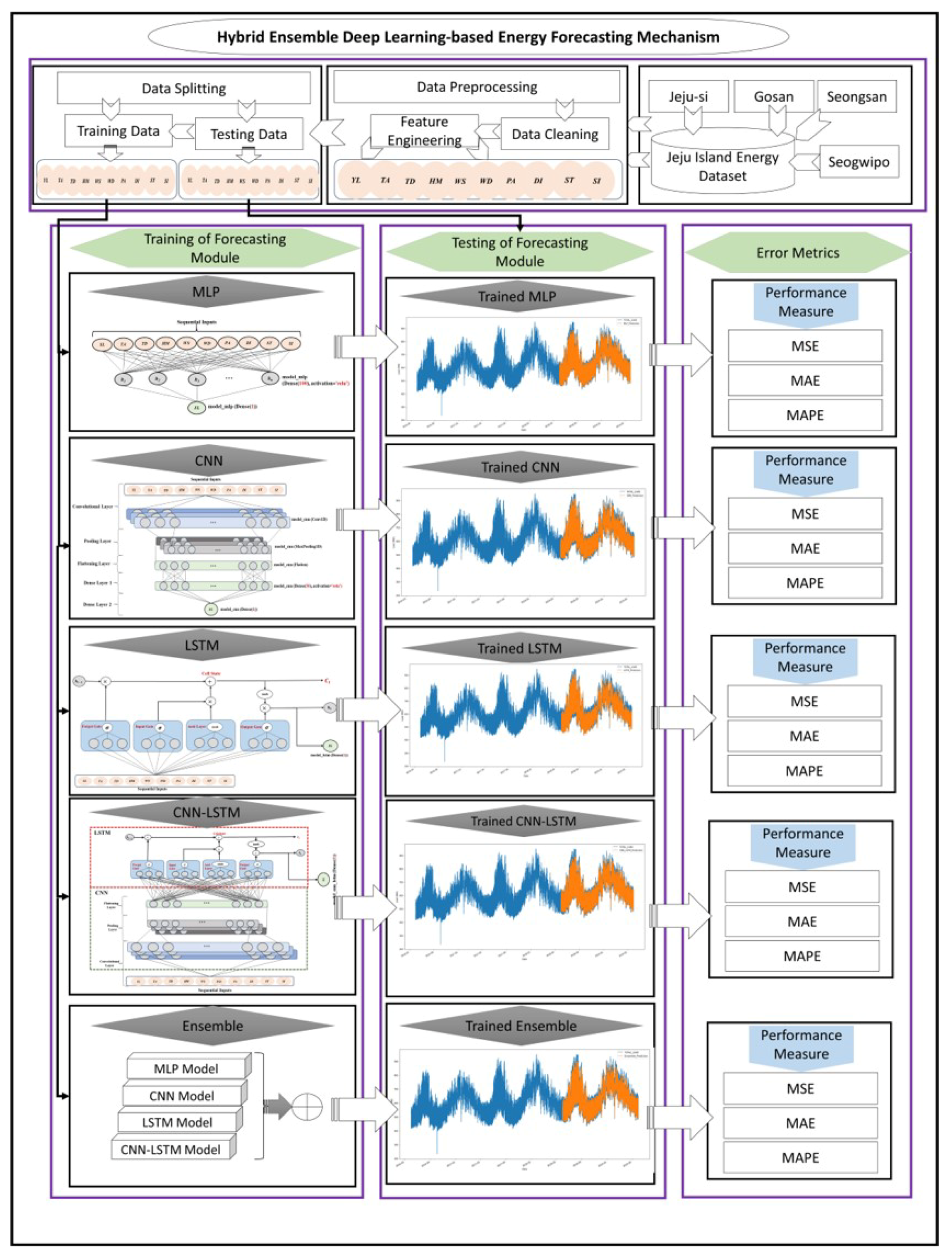
2.5.3. The Proposed System
The framework of the hybrid ensemble deep learning-based energy forecasting mechanism is represented in
Figure 7. A detailed explanation of the six steps in the proposed system is described as follows:
Step 1: Data collection
The energy data and weather information are collected hourly from four regions in Jeju Island. The weather data are averaged according to the portion of each region. Therefore, this study uses the total load and total weather data of the whole Jeju.
Step 2: Data preprocessing
Some information is missing in our raw data, so we cleaned the original data using the specific data average. After cleaning and removing missing values, we selected ten inputs based on the data correlation and then arranged the input data.
Step 3: Data Splitting
The arranged data are split into two portions: training and testing. Two-year training from June 2016 to May 2018 and one-year testing from June 2018 to May 2019 are utilized for training and testing all proposed models.
Step 4: Training of forecasting module
After we get the training and testing sets, training data are given to each DL model. Before training, input data are transformed into sequential data to feed as sequencers and converted into a supervised learning format. Therefore, the sequential data are used for all proposed DL models. Four DL models such as MLP, CNN, LSTM, and hybrid CNN-LSTM are then defined and fitted in the training data.The parameters mentioned above in the last subsection are used for building these models. Successively, these four models are ensembled to make ensemble predictions.
Step 5: Testing of forecasting module
Testing data is provided to the trained models once learned from the training data. Afterward, predictions on the testing data are completed for each DL model and the proposed ensemble model.
Step 6: Error Measurement
The last phase measures the forecasting performance that indicates how much forecast value differs from the corresponding observation. To do so, we select three error metrics, including mean squared error (
MSE), mean absolute error (
MAE), and mean absolute percentage error (
MAPE), which are commonly used for measuring the forecasting accuracy. The mathematical formulas for these error metrics are expressed as:
where,
= an actual energy at time
t,
= a predicted energy at time
t,
.
3. Experimental Results
The generated results between the proposed ensemble model and other DL stand-alone models are compared monthly error metrics on test predictions from June 2018 to May 2019. Monthly MSE, MAE, and MAPE are evaluated to make a comparison among all models, as revealed in
Table 3,
Table 4 and
Table 5, respectively. In general, our proposed model outperforms other DL models, showing 1472.76 MSE, 28 MAE, and 4.15 MAPE. All models provide reasonable forecast values, with errors varying from 3% to 5% of MAPEs in all months, except February. Our proposed DL ensemble model is ranked first, showing better accuracy in June, August, September, March, and April, followed by the MLP model, which gives better performance in October and December. The hybrid CNN-LSTM and CNN models execute almost similar percentages, at 4.26% and 4.27% in the total average of test forecasts. The LSTM model is ranked last with the average 4.34% MAPE, 29.13 MAE, and 1459.68 MSE, while there are better accuracies of LSTM in July and February.
Four different groups consisting of weekdays, weekends, Mondays, and holidays are divided to further MAPE comparison among all models.
Table 6 is referred to the comparison of average MAPEs of each category for both proposed and baseline models. In general, the group on weekdays performs lower MAPE than other groups, with around 3% in all models. Considering the weekday category, the proposed model provides the lowest MAPE with 3.39% among all DL models. It also generates lower MAPE than others in the group of weekends, amounting to 4.04%. However, the ensemble model contributes approximately 0.1% higher than the LSTM model in the groups of Mondays and holidays.
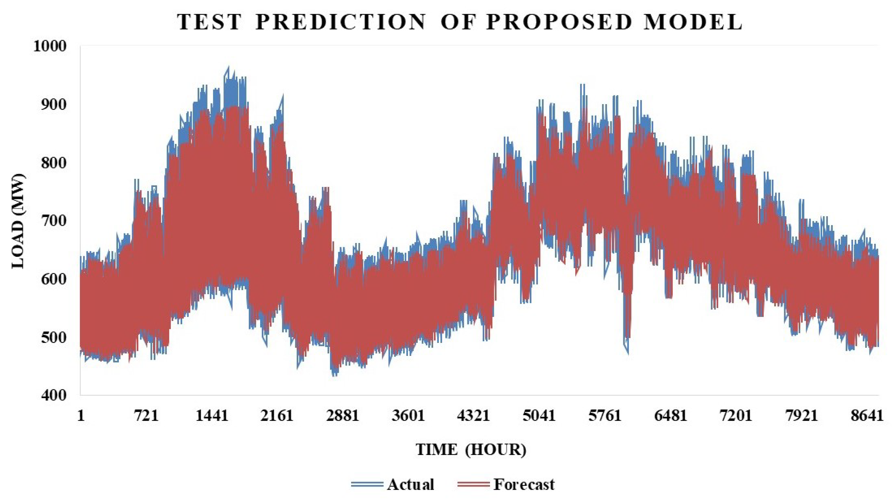
The actual energy versus forecast energy of the proposed model on testing data is indicated in
Figure 8. The forecast of the proposed model closely follows the actual energy. The
x-axis of the figure represents the hourly period from June 2018 to May 2019, whereas the
y-axis indicates the load in the megawatt units (MW). The blue line shows the actual energy, whereas the red line is indicated as the forecast results. As shown in the figure, there is a big gap between actual and forecast in July, ranging in time from 721 to 1440 due to the high temperature. Apart from this, the proposed model predicts the actual load accurately.
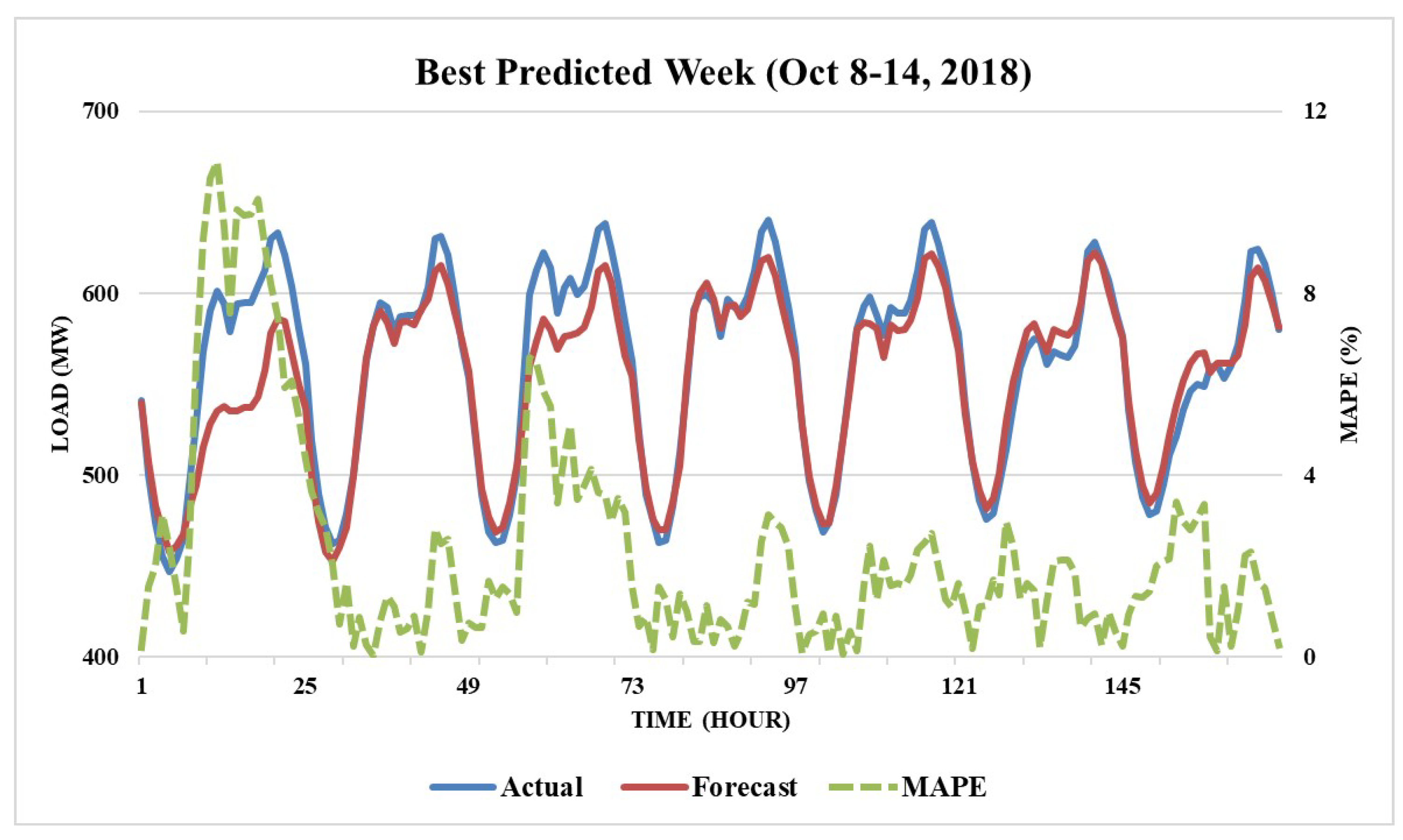
To the extent of better visualization in predicted results, the best predicted week and the best predicted day from test predictions are visualized in
Figure 9 and
Figure 10, correspondingly. Both figures have a primary
x-axis in an hour, a
y-axis in MW, and a secondary
y-axis in the percentage of MAPE. Regarding lines in both figures, blue represents the actual load, while red is the forecasted MW load. Moreover, another green line refers to the MAPE measurement. The best predicted week is the second week of October 2018, as seen in
Figure 9. The load fluctuations between actual and forecast are almost similar, ranging from 400–640 MW. The proposed model conducts under forecast, which is suitable for forecasting. Although there are high errors for some points on 8 October 2018, the model predicts better values for the other days of the week. MAPEs vary from 1.24% to 1.64%, except 6.23% on October 8 and 3.28% on October 10.
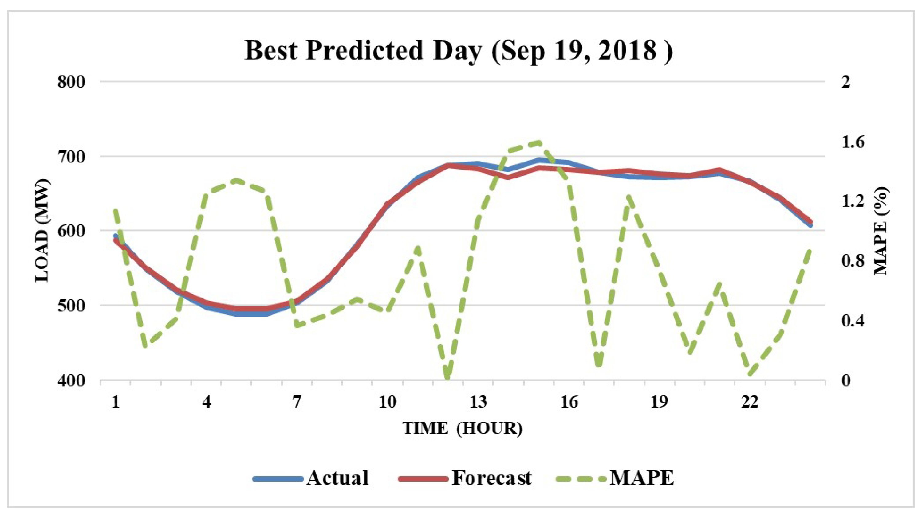
Similarly, the best predicted day is selected to realize how much minimum error the proposed model can forecast. Like
Figure 9, three lines show actual, forecast, and MAPE in
Figure 10. The minimum MAPE at 0.75% is executed on 19 September 2018. The errors range from 0.001% at 11 AM to 1.593% at 2 PM in a day. The pattern of forecast values fluctuates similarly to that of actual values. Therefore, our proposed ensemble model is a promising model providing an acceptable and reliable result for time series prediction.
For further comparison, we chose the existing paper conducted similar to our work and compared our results and their results [
32]. Their research proposed the stochastic ensemble model framework formulated as a two-stage random forest problem with a series of homogeneous prediction models. In their study, three load consumption datasets such as the Korean Electric Power Company (KEPCO) substation building, the Korean Research Institute (KEPRI) building, and testbed were applied to train their proposed ensemble model. However, we select the MAPE results from their first two datasets to compare with our results.
Table 7 indicates the seasonal MAPE comparison between their proposed model and our proposed model. According to previous work, MAPEs for each season are computed to make further comparisons. Our proposed DL ensemble model outperforms the cited proposed ensemble model by providing 4.20% in Spring, 3.77% in Summer, 3.48% in Fall, and 5.22% in Winter. Nevertheless, we can reveal that the proposed ensemble model from both works could predict the load consumption as accurately as the actual energy by comparing it with other stand-alone forecasting models.


