Optimal Scheduling of Microgrid Considering the Interruptible Load Shifting Based on Improved Biogeography-Based Optimization Algorithm

Abstract

A microgrid is an efficient method of uniting distributed generations. To ensure the applicability and symmetry of the microgrid, the environmental benefits and economic costs are considered to comprehensively model the optimal operation of the microgrid under the grid-connected operation mode, at the same time, considering the effect of interruptible load on the operating cost of the microgrid, the power shifting for interruptible load is attempted on the basis of battery storage capacity. By adaptively adjusting the migration rate using the habitat suitability index of a normalized individual and adding a certain differential perturbation to the migration operator of the migration mechanism, an improved biogeography-based optimization algorithm is proposed and the microgrid optimization dispatching algorithm based on the improved biogeography-based optimization is applied. The advancement and effectiveness of the proposed algorithm and model is verified by the example, and the simulation results indicate that the implementation of the power dispatching scheme proposed in this paper can effectively reduce the total cost of the system. Moreover, the proper consideration of shifting interruptible load, the effective load management and guiding the electricity consumption behavior of users are of certain significance for optimizing the utilization of renewable energy and improving the system efficiency and economy.

1. Introduction

With global warming and the depletion of energy, renewable clean energy, which includes wind and solar power, has gradually attracted people’s attention. However, uncontrollable factors of renewable energy caused by the randomness and intermittence of wind energy and light intensity seriously affect the stability and reliability of the grid operation. At the same time, it is difficult for a power system with only several renewable energy generations to meet the load demand in isolated islands. Hence, a microgrid, which combines distributed micro power supply, load unit, energy storage unit and control equipment, can deal with the above problems well. It has become a hot research topic for many scholars to reasonably optimize a microgrid system to achieve economic and environmental optimization.

Firstly, in the field of microgrid energy system optimization, research topics in large numbers focus on the optimization of the output power or economic model [1,2,3], the improvement of evolution strategy or the optimization of the control system [4]. To be specific, distributed power generation scheduling problems are usually nonlinear and non-convex multi-objective optimization problems [5]. It is difficult for traditional optimization algorithms and mathematical methods dealing with convex functions to solve such problems. Most intelligent optimization algorithms, which include the particle swarming algorithm (PSO) [6,7,8], the genetic algorithm (GA) [9,10] and the bacterial foraging algorithm (BFA) [11], have different optimization effects in different fields. In recent years, intelligent optimization algorithms in large numbers have been widely used in the power dispatching of a microgrid. With the continuous efforts of many scholars, optimization algorithms have developed different evolution strategies. In [12], the optimization model of a microgrid, considering the economy, environment and system operation risks, is built, and a multi-objective particle swarm algorithm based on niche technology is used to deal with this model. In [13], a microgrid system combined heat and power is presented, which reduces the operating cost of the microgrid by recycling the waste heat in the system. In [14], to better deal with the energy efficiency and pollutant emission problems of the microgrid, fuzzy processing technology and tabu search are introduced and an improved particle swarm optimization algorithm is proposed. In [15], the traditional niche technology is improved in the elimination rule of individual fitness, in order to propose an improved genetic optimization algorithm. In [16], the environmental treatment cost, maintenance cost and operating cost of the microgrid system are considered separately, and the multi-objective optimization model is converted into a single-objective optimization model by adding the weight coefficient, and the optimization results obtained by different weight coefficients are analyzed. In [17], the optimal configuration model is established, which included the investment cost of equipment, environmental protection cost, operation cost, maintenance cost and fuel cost, and the improved bacterial foraging algorithm (BFA) is used to deal with the problem of optimal configuration for the hybrid island operation of a microgrid. In [18], considering several objectives including economic benefits, network loss and environmental costs, by introducing elite strategy, reverse learning mechanism and global memory, a microgrid optimization operation method based on advanced gravitational search algorithm is applied. In [19], considering the security, economy and environmental protection of the microgrid, the three indicators, which include the microgrid system’s voltage stability, active power loss and gas pollution, are quantitatively evaluated, and the microgrid optimization model is established; the strength Pareto evolutionary algorithm proposed solves this model. In [20], based on the theory of chance-constrained programming, a dynamic economic dispatch model of the microgrid with wind farms considering microgrid operation risk constraints is established, and a hybrid intelligent optimization algorithm combining sequence operation theory and a genetic algorithm is proposed to solve the model. In [21], by modeling the uncertainty of light power and wind power, an Adaptive Modified Firefly Algorithm (AMFA) is proposed. Many of the various algorithms mentioned above consider economic and environmental factors, but they do not consider load optimization strategies. For this reason, a multi-objective optimization strategy considering interruptible load shifting is proposed in this paper.

A biogeography-based optimization (BBO) algorithm, proposed by American scholar Dan Simon [22], is a swarm intelligence optimization algorithm based on biogeography theory. Compared with the PSO and GA algorithms, BBO has some advantages in convergence performance, and the ability of this algorithm in optimization has currently been verified by expert scholars through experimental studies. However, the basic BBO still suffers from premature convergence and faces the problem of local optimization; it still needs to be improved to further enhance its optimization performance. The optimization of the typical daily microgrid system in summer involves the output power of a micro gas turbine, photovoltaic array, fuel cell, storage battery and wind turbine. An optimal scheduling model of the microgrid considering the economic and environmental protection under the grid-connected operation mode is established on the premise of meeting the load demand and system constraints. Meanwhile, for the consumer side, considering the symmetry of interruptible load and the operating cost in the microgrid system, the power shifting for interruptible load is attempted on the basis of the battery storage capacity in this paper. Through simulation experiments, the comprehensive optimal scheduling of the microgrid is obtained, and compared with the basic BBO and other two algorithms, the performance of the proposed method surpasses the other methods mentioned above, which provides an effective means to solve the optimal operation of the microgrid with an intelligent optimization algorithm. The proper consideration of shifting interruptible load, the effective load management and guiding the electricity consumption behavior of users are of certain significance for optimizing the utilization of renewable energy and improving system efficiency and economy.

2. Multi-Objective Optimization Operation of Microgrid under Grid-Connected Mode

The microgrid power generation units used in this paper are mainly divided into renewable energy units and non-renewable energy units. Among them, renewable energy power units include photovoltaic cells (PV) and wind turbines (WT) with uncontrollable power generation; non-renewable energy units are composed of micro gas turbines (MT) and fuel cells (FC) with controllable power generation. Through the coordinated use of the above units under different constraints, the optimization of environmental benefit and economic cost can be obtained.

2.1. System Power Generation Models

2.1.1. Model of WT Generator

The specific output formula of a wind turbine is shown in Equation (1):

$$P_{WT}=\{\begin{array}{l}0,v\le v_{ci},v>v_{co}\\ P_v,v_{ci}<v\le v_{co}\end{array}$$

(1)

where v is the current wind speed and v_ci and v_co are the minimum and maximum wind speeds required for the normal operation of the wind turbine. When the current wind speed is between v_ci and v_co, P_v is the output of the WT.

2.1.2. Model of PV Generator

The output of photovoltaic generator, which is based on light intensity and ambient temperature, is shown in Equation (2) as follows:

$$P_{PV}=P_S\frac{S_A}{S_0}\left(1+k\left(T_c-T_r\right)\right)$$

(2)

In Equation (2), P_s represents the maximum output power of PV; S_A and S_o represent the ambient light intensity during the scheduling period and the light intensity under the rated power, respectively; k represents the ambient temperature coefficient; T_C represents the actual temperature of the PV board during the dispatch period; and T_r represents the reference temperature under standard conditions.

2.1.3. Model of MT Fuel Cost

The micro gas turbine (MT) fuel cost can be calculated as Equation (3) as follows:

$$F_{MT}=C_{fuel}\frac{1}{L}\frac{P_{MT}}{{\eta }_{MT}}$$

(3)

where F_MT is the MT fuel cost; C_fuel and L are the real-time price of fuel gas and the low calorific value of fuel gas, respectively; and P_MT and η_MT are the actual output and the working efficiency of the micro gas turbine, respectively.

2.1.4. Model of Fuel Cell Cost

A fuel cell is a piece of electrochemical equipment that reacts hydrogen with oxygen or other oxides. The principle of fuel cell power generation is that the chemical energy of fuel is converted into electrical energy [23]. The main discharge of a fuel cell is water, there are no pollutants such as CO and NO_x, and its power generation efficiency is high; therefore, it is widely used in the field of power systems.

The fuel cost model of the fuel cell is similar to the fuel gas cost model of the micro gas turbine in Equation (3); therefore, it can be given by the following:

$$F_{FC}=C_{fuel}\frac{1}{L}\frac{P_{FC}}{{\eta }_{FC}}$$

(4)

where F_FC represents the fuel cell cost, and P_FC and η_FC represent the output and working efficiency of the fuel cell, respectively.

2.1.5. Model of Storage Battery

Considering the uncertainty of renewable energy in the optimal scheduling of the microgrid, such as a WT generator and a PV generator, storage batteries are added to maintain the stability of the microgrid operation and minimize the economic loss by overload. The model of the state of charge of a battery (SOC) is established, which represents the radio of the current remaining power of the battery to the total capacity of the battery. The specific formula is expressed as follows.

The charging formula of storage battery can be calculated as follows:

$$SO{C}_{t+1}=(1-\sigma )SO{C}_t+(P_{ES,t}\Delta t{\eta }_{IN})/C$$

(5)

where SOC_t and SOC_t+1 are the state of charge of the battery at time t and time t + 1; σ represents the self-discharge coefficient of the storage battery; P_ES,t is the charge–discharge power at time t. When the battery is charging, P_ES,t > 0, when the battery stops, P_ES,t = 0, otherwise P_ES,t < 0. η_IN represents the charge efficiency of the storage battery and C is the maximum charging capacity of the storage battery within unit time ∆t.

The discharging formula of storage battery can be calculated as follows:

$$SO{C}_{t+1}=(1-\sigma )SO{C}_t-P_{ES,t}\Delta t/(C{\eta }_{OUT})$$

(6)

where all the symbols represent the same as they did in Equation (5) and η_OUT represents the discharge efficiency of the storage battery.

2.2. The Key Technologies for Optimal Dispatch of Microgrid

The aim of the optimal dispatch of the microgrid is to achieve the minimum economic cost and environmental cost by rationally dispatching the output power of different distributed power generation units and satisfying various power constrains and load requirements.

2.2.1. The Objective Function

• Cost of the operating

As one of the most important optimization indexes in the microgrid optimization dispatching, the microgrid operating cost plays an important role in measuring the feasibility and applicability of the microgrid system. It includes the fuel cost and the maintenance cost of each generator, as well as the online electricity cost. The specific formula can be defined as the following Equation (7):

$$\min F_1={\displaystyle {\sum }_{t=1}^T{\displaystyle {\sum }_{i=1}^N(C_{{}_{F,i,t}}+C_{{}_{OM,i,t}}+n{C}_{{}_{G,t}})}}$$

(7)

where F₁ represents the total cost of system operation; T is the number of unit scheduling intervals of the system during a scheduling period, in this paper, T is 24; N is the total number of various power generators; C_F,j,t and C_OM,j,t are the fuel cost and the maintenance cost of the i-th generator in the t-th time interval, respectively; C_OM,I,t = k_OM,I P_i,t, k_OM,I and P_i,t are the loss coefficient and the output of the i-th generator in the t-th time interval, respectively; and C_G,t represents the online electricity cost at time t. When the microgrid is running in the grid-connected operation mode, n = 1.

• Cost of pollution

With global warming, people have comprehensively promoted the sustainable development strategy, and the cost of pollution has become an important part of the total cost of the microgrid. The pollution index in this paper is the pollution degree judgment made by the pollution of CO, SO₂, Nox and other pollutants discharged by non-clean energy units, such as micro turbines and fuel cells. Since clean energy units, which include photovoltaic cells (PV) and wind power (WT), do not discharge pollution gas, they can be neglected in this pollution cost. The minimum pollution cost formula can be given by the following:

$$\min F_2={\displaystyle {\sum }_{t=1}^T{\displaystyle {\sum }_{j=1}^M{C}_j{\displaystyle {\sum }_{i=1}^N{K}_{ij}}{P}_{i,t}}}$$

(8)

where F₂ represents the total cost required to treat the pollutants emitted by the microgrid; M represents the number of pollutant types; C_j represents the treatment cost corresponding to the pollutant j; K_ij represents the treatment coefficient of the pollutant j discharged by the i-th generator; P_i,t represents the output of the i-th generator during the t-th time period.

In addition, the calculation formula of the comprehensive cost can be obtained by linearly weighting the operating cost and the environmental governance cost, which transforms the multi-objective non-convex optimization problem into a single-objective optimization problem for the microgrid.

2.2.2. Constraints

The above models should satisfy the following constraints:

• The total power constraint;

  $${\displaystyle {\sum }_{i=1}^N{P}_{i,t}}+P_{ES,t}+P_{Grid,t}-P_{L,t}=0$$

  (9)

  where P_i,t represents the output power of the i-th micro energy unit at time t; P_ES,t represents the charge–discharging power of the storage battery at time t, when the battery is discharged, P_ES,t < 0; P_Grid,t represents the interactive power between the large grid and the microgrid at time t. When the load is overloaded, the microgrid purchases electric energy from the large grid, P_Grid,t > 0; P_L,t represents the total power consumption on the load side at time t.
• The output power constraint of micro energy generator unit;

  $$P_{i\min }\le P_i\le P_{i\max }$$

  (10)

  where P_imin and P_imax represent the upper limit and the lower limit of the i-th unit output.
• The transmission power constraint;

  $$0\le P_{Grid}\le P_{Grid\max }$$

  (11)

  where P_Gridmax is the maximum allowable transmission power between the microgrid and the distribution grid.
• The climbing rate limit;

The constrain of load increases is as follows:

$$P_{i,t}-P_{i,t-1}\le R_{iup}$$

(12)

The constrain of load reduction is as follows:

$$P_{i,t-1}-P_{i,t}\le R_{idown}$$

(13)

As can be seen from Equations (12) and (13), the climbing speed of the i-th generator is bounded by the upper R_iup and lower R_idown generation limits.

• Energy storage battery constrains.

Considering the security of the storage battery, its state of charge must be bounded within the minimum and maximum.

$$SO{C}_{i\min }\le SO{C}_{i,t}\le SO{C}_{i\max }$$

(14)

where SOC_imin and SOC_imax are the allowable minimum and maximum battery states of the charge.

2.2.3. The Objective Function Added the Interruptible Load Shifting

The operation optimization of the microgrid is the basis for ensuring the high-quality and efficient operation of the microgrid. In the above, the comprehensive cost of microgrid optimal operation is determined by the combination of operating costs and environmental costs. Then, for the consumer side, considering the effect of interruptible load on the operating cost of the microgrid, the power shifting for interruptible load is attempted with certain constraints.

According to the actual situation, the load can be divided into non-interruptible load and interruptible load. The microgrid needs to meet uninterruptible load, and the interruptible load can attempt to shift to the time when the original demand for electricity is lower. Since the shifting of interruptible load can have certain impact on the use of electricity for the original user side, the amount of load involved in the shifting and the time span of shifting are both issues to be considered. Consequently, considering the impact on the user side in terms of the total amount of power shifting and the shifting time, a comprehensive evaluation objective function with the power shifting of the interruptible load is established in this paper, as shown in the following Equation (15):

$$F=(F_1+F_2)(1+\frac{P_{LS}}{P_{LI}+P_{LU}})(1+\alpha Ts)$$

(15)

where F is the comprehensive evaluation objective function with interruptible load shifting. $P_{LS}/\left(P_{LI}+P_{LU}\right)$ is the penalty term of the total shifting load on the total optimization cost. Only when the optimization cost after load shifting is better than the original cost after penalty, can power shifting be carried out. $P_{LS}$ is the interruptible load involved in shifting, $P_{LI}$ is the maximum shifting load of daily interruptible load, $P_{LU}$ is the demand power of non-interruptible load and $P_{LI}+P_{LU}=P_L$. Obviously, when the load is not shiftable, the comprehensive evaluation objective function F = F₁ + F₂, which is equal to the comprehensive optimization cost mentioned above. $\alpha$ is the adjustment factor of shifting time, and Ts is the total shifting time; the pseudo code for the total shifting time is shown in Algorithm 1.

Algorithm 1 The Calculation of the Total Shifting Time.

Let $P_{LS{I}_i}$ be the i-th load shifted in and $P_{LS{O}_j}$ be the j-th load shifted out, where i $\in \left[1,i_{\max }\right],$ $j\in \left[1,j_{\max }\right]$, $I_i$, and $O_j$ are the current time corresponding to the respective load, $I_i,O_j\in \left(0, 24\right).$ Then, ${{\displaystyle \sum }}_{i=1}^{i_{\max }}{P}_{LS{I}_i}=\left|{{\displaystyle \sum }}_{j=1}^{j_{\max }}{P}_{LS{O}_j}\right|=P_{LS}\le P_{LI}$; set $P_{LSm}$ as the maximum load of single time shifting; the formulas $P_{LS{I}_i}\le P_{LSm}$ and $\left|P_{LS{O}_j}\right|\le P_{LSm}$ need to be satisfied. Set $i=1$, $j=1$. Calculate the cumulative sum of $P_{LS{I}_i}$ and add to $P_{LS{O}_j}$ to satisfy ${{\displaystyle \sum }}_{i=1}^{i_{max}}{P}_{LS{I}_i}+P_{LS{O}_j}\ge 0$; record $i_{m_j}.$ Then, the shifting time $t_j$ of the load shifted corresponding to the j-th load shifted in is $t{s}_j=O_j-\frac{1}{i_{m_j}-i+1}{{\displaystyle \sum }}_i^{i_{m_j}}{I}_i.$ $\{\begin{array}{l} When{{\displaystyle \sum }}_{i=1}^{i_{m_j}}{P}_{LS{I}_i}+P_{LS{O}_j}=0,i=i_{m_j}+1,j=j+1.\\ When{{\displaystyle \sum }}_{i=1}^{i_{m_j}}{P}_{LS{I}_i}+P_{LS{O}_j}>0,P_{LS{I}_{i_{m_j}}}={{\displaystyle \sum }}_{i=1}^{i_{m_j}}{P}_{LS{I}_i}+P_{LS{O}_j},i=i_{m_j},j=j+1.\end{array}$ Repeat steps 4–6, until $t{s}_{j_{\max }}$ is obtained. Then, the total shifting time Ts = ${{\displaystyle \sum }}_{j=1}^{j_{\max }}t{s}_j$.

Considering the degree of effect of the power shifting time on the user side, the calculation of the total shifting time Ts is added. According to the formula, compared with the original power demand time and the power consumption time after shifting, the more time that is shifted, the greater the total shifting time Ts is, and vice versa. For the time factor $\alpha$, the greater the time factor $\alpha$ is, the higher the penalty degree of shifting time Ts on the comprehensive operating cost is, which can force the power to shift to the closer time of the original power demand time. However, when the value of $\alpha$ reaches a certain threshold, even though the comprehensive operating cost of the microgrid after power shifting can be lower, the microgrid scheduling scheme with power shifting cannot be obtained due to the penalty relation of shifting time Ts. Therefore, the objective function, which comprehensively considers the operating cost, environmental cost and user-side demand of the microgrid, is established on the basis of the mutual coordination of the various distributed generation and full consideration of battery charging and discharging capacity, which can more effectively maximize the use of renewable clean energy and, thus, realize the maximum operation benefit of the microgrid.

3. Biogeography-Based Optimization Algorithm

Biogeography is an independent discipline that studies the temporal and spatial distribution of biological communities and their components, which originated in the 19th century. Scholars in large numbers around the world have made in-depth research on it, and numerous mathematical models for the distribution, migration and extinction of biological communities have been proposed. Inspired by these mathematical models, biogeography-based optimization (BBO) was proposed by American academic Dan Simon in 2008. According to the mathematical model of species migration, BBO depends on the simulation of a species migration mechanism among habitats to achieve the goal of finding the global optimal solution.

3.1. The Basic Biogeography-Based Optimization Algorithm

Nowadays, the BBO algorithm is involved in various fields, including biology [24], environmental science [25], etc. In BBO, the habitats of species in biogeography correspond to the possible individuals of optimization problems, the suitability index variables (SIV) in the model correspond to individual variables, and the habitat suitability index (I) corresponds to the fitness function of evaluating the quality of a solution set. When solving optimization problems, multiple habitats are randomly generated as the initial solution of the optimization problem. Through the information exchange of species migration between habitats, the species diversity of habitats is improved, the I of habitats is improved and then the optimal solution of the problem is obtained. The key steps of BBO are as follows: initialization, migration and mutation.

• Initialization

The parameters of the BBO algorithm are initialized, including the maximum number of species per habitat S_max, the maximum allowable immigration rate I and emigration rate E and the maximum mutation rate m_max. The BBO algorithm randomly generates N habitats as the initial population using Equation (16), and each habitat as a potential solution contains D-dimensional solution variables. Afterwards, the I for each habitat is calculated.

$$x_{ij}=x_{j,\min }+rand(x_{j,\max }-x_{j,\min })$$

(16)

where x_ij is the j-th dimensional solution variable of habitat x_i, i ∈ [1, 2, …, NP], j ∈ [1, 2, …, D]; and x_j,max and x_j,min are the lower and upper limits of the j-th dimensional variable, respectively.

• Migration

The BBO algorithm exchanges information with other habitats through the migration mechanism, and then the solution space is searched in a wide area. Based on the basic principles of biogeography, the I of habitat is directly proportional to species diversity, and the habitat with a higher I can accommodate more species. Therefore, there is the mapping relationship between habitat x_i and the number of species S_i. After reordering x_i according to its corresponding I from high to low, the original habitat x_i is given a new i. The number of species S_i of x_i after ranking is calculated using Equation (17).

$$S_i=S_{\max }-i$$

(17)

As can be seen from the mechanism of biogeographical species migration, the specific formula of the immigration rate λ_i and the emigration rate μ_i of habitat x_i can be given by the following:

$$\{\begin{array}{l}{\lambda }_i=I(1-\frac{S_i}{S_{\max }})\\ {\mu }_i=\frac{E\cdot S_i}{S_{\max }}\end{array}$$

(18)

In the migration operation, firstly, the habitat x_i to be migrated is determined according to the migration rate λ_i. A random number between (0,1) is generated, if it is less than λ_i, then the habitat x_i is that to be moved in. Next, for each dimension of x_i, the habitat with which to migrate needs to be determined. Among the remaining N − 1 habitats, x_k is determined by roulette according to their migration rate μ_k. Finally, the solution variables of habitat x_i are replaced by the solution variables of the selected habitat x_k.

• Mutation

A habitat may mutate its I due to a catastrophic event and the BBO algorithm uses a mutation operation to simulate the rapid change of I in a habitat caused by such an emergency. According to the immigration rate λ_i and the emigration rate μ_i, the probability P_i of species number S in habitat x_i is calculated using Equation (19).

$$P_i=\{\begin{array}{ll}-({\lambda }_i+{\mu }_i)P_i+{\mu }_{i+1}{P}_{i+1},\hfill & S_i=0\hfill \\ -({\lambda }_i+{\mu }_i)P_i+{\lambda }_{i-1}{P}_{i-1}+{\mu }_{i+1}{P}_{i+1},\hfill & 1\le S_i\le S_{\max }-1\hfill \\ -({\lambda }_i+{\mu }_i)P_i+{\lambda }_{i-1}{P}_{i-1},\hfill & S_i=S_{\max }\hfill \end{array}$$

(19)

The mutation rate m_i of habitat x_i is calculated using Equation (20).

$$m_i=m_{\max }(1-\frac{P_i}{P_{\max }})$$

(20)

where m_max is the maximum mutation rate of the habitat and P_max is the maximum probability of all species.

3.2. Improved BBO Algorithm

• Adaptive determination mechanism of migration rate

The determination of the immigration and emigration rate in BBO can only reflect the order of individual quality, while ignoring the evolutionary state of the current population and failing to rationally assess the quality of individuals. Once individuals have large quality gaps or are unevenly distributed, it is easy to make an incorrect assessment of the degree of the individual’s quality, resulting in the beneficial information of the better individual unable to be retained, or the poor individual who participated early in evolution. Based on the above question, this paper uses the I value of normalized individuals to adjust the immigration rate adaptively, as shown in Equation (21).

$$\{\begin{array}{l}{\lambda }_i=(\frac{F_i-F_{\min }}{F_{\max }-F_{\min }})\\ {\mu }_i=1-{\lambda }_i\end{array}$$

(21)

where F_i is the I of habitat x_i and F_max and F_min are the maximum and minimum value of I in the current population. This method can solve the problem that individual quality cannot be monitored in real time while ensuring the effective use of information about individuals in the current population and evaluate the individuals to be immigrated or emigrated more accurately.

• Dynamic migration mechanism

The migration strategy of BBO as an important part of its evolution mechanism, to a large extent, affects the performance of the algorithm. However, its migration method of directly replacing the SIV of the original solution with the SIV to be emigrated, may lead to a certain blindness in migration, and the poor ability of mining new solutions, which can easily cause premature convergence. Therefore, a new dynamic migration mechanism is employed to solve this problem, which uses an adaptive migration rate designed in the previous section to adjust the degree of perturbation of the differential vector for mining new solutions, in order to achieve adaptive perturbation around the SIV to be emigrated at different evolutionary periods, thus enhancing the search capability of the migrating algorithm, as shown in Equation (22).

$$x_{ij}=x_{kj}+(r_{\min }+{\lambda }_i\times (r_{\max }-r_{\min }))\times (x_{aj}-x_{bj})$$

(22)

where x_k is the habitat to be emigrated; a and b are random numbers among [1, NP]; then, x_aj and x_bj, respectively, represent the j-th dimensional variables of the a-th and the b-th habitat; and r_max and r_min are the maximum and minimum disturbance degree, respectively.

3.3. The Algorithm Flow

The specific operation process of microgrid optimization based on the improved BBO (IBBO) algorithm can be clearly expressed through the following eight steps.

Step 1. Describe the actual power data and system parameters of the microgrid, such as the output of photovoltaic and wind turbine, power demand on the side, etc. In addition, the output of each distributed power generation and battery needs to be limited. Then, define the general parameters of the IBBO algorithm, including S_max, I, E and m_max.

Step 2. Set the population size NP, and random population H = {x_i, I = 1, 2, …, NP}. Each individual in the population H is determined by the micro power supplies in different scheduling times and the dimensions of the individual are equal to (N + 1) × t. N represents the total number of those distributed generators, and t represents the total time for the optimal dispatch of the microgrid. The last row is the shifting amount of the corresponding scheduling time when considering load shifting. Certainly, when the load is not shiftable, no matter what the row value is, it does not affect the output results of each micro power supply at each scheduling time.

Step 3. Evaluate the HSI of the current habitat individuals, eliminate individuals that do not meet the constraints and sort the remaining habitat individuals in ascending order according to HSI and use them as population H.

Step 4. From Equation (21), calculate the value of λ_i and μ_i for each habitat x_i in the population H separately.

Step 5. Substitute the parameters λ_i and μ_i into Equation (22) to obtain the migration.

Step 6. Determine the mutation rate m_i and species probability P_i in each habitat. According to the mutation rate of each habitat, make mutation for species.

Step 7. Judge whether the obtained population meets the requirements, if not, continue to the next iteration and go back to stage three, else execute the next stage.

Step 8. Print the optimal habitat population H.

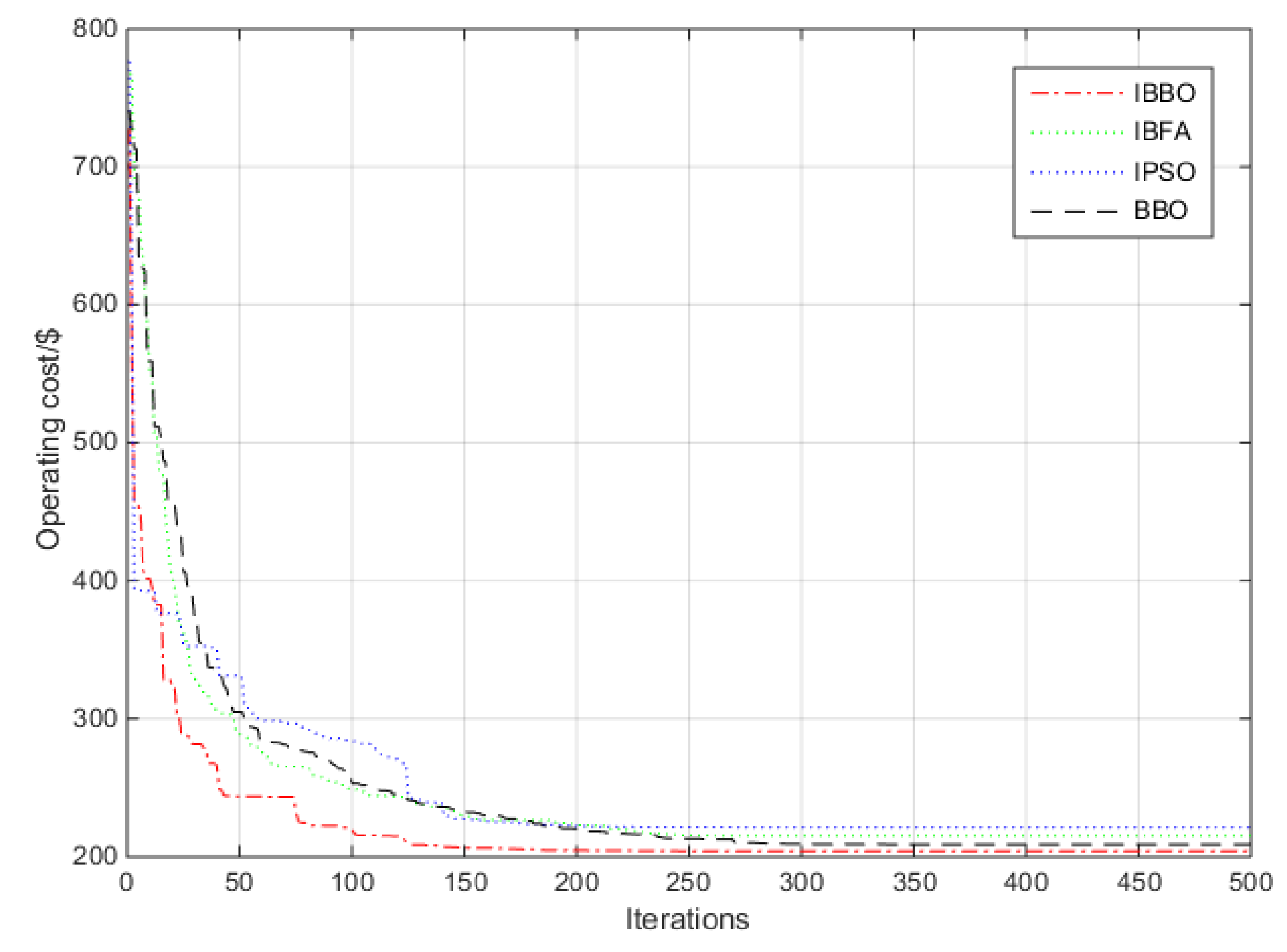
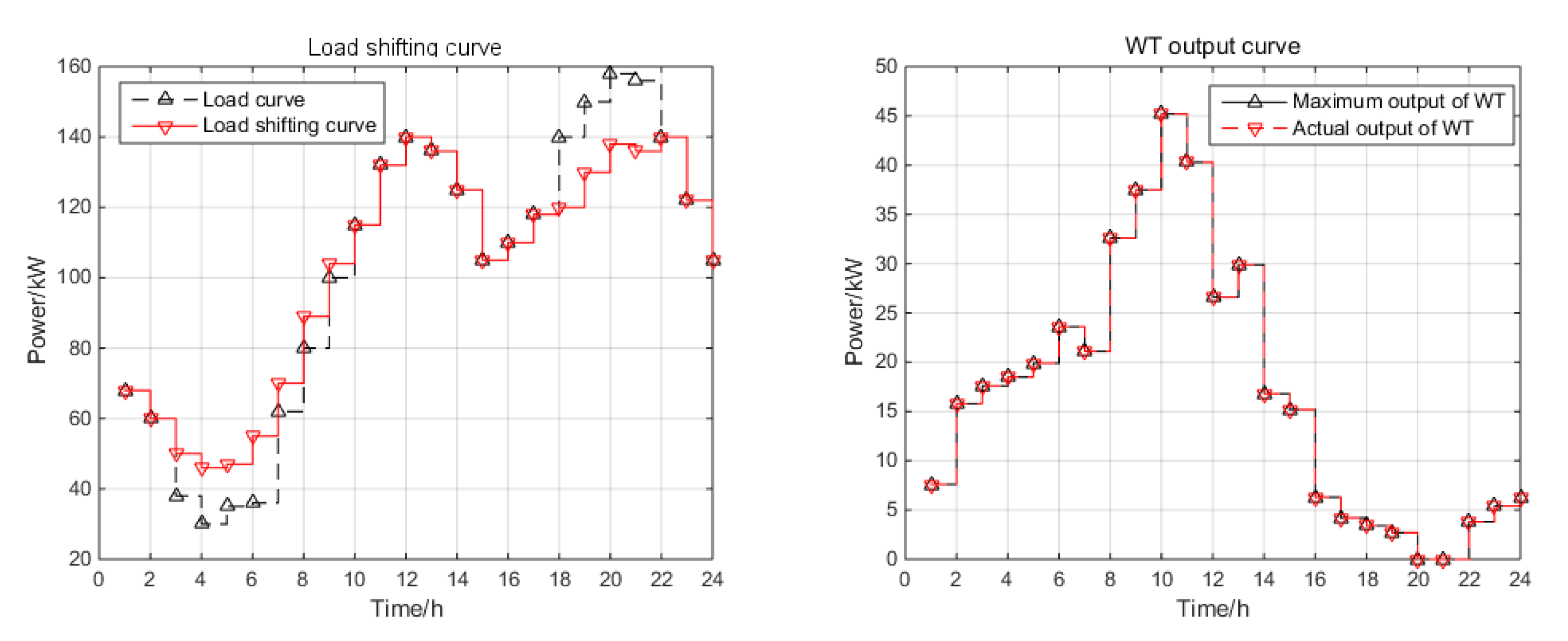
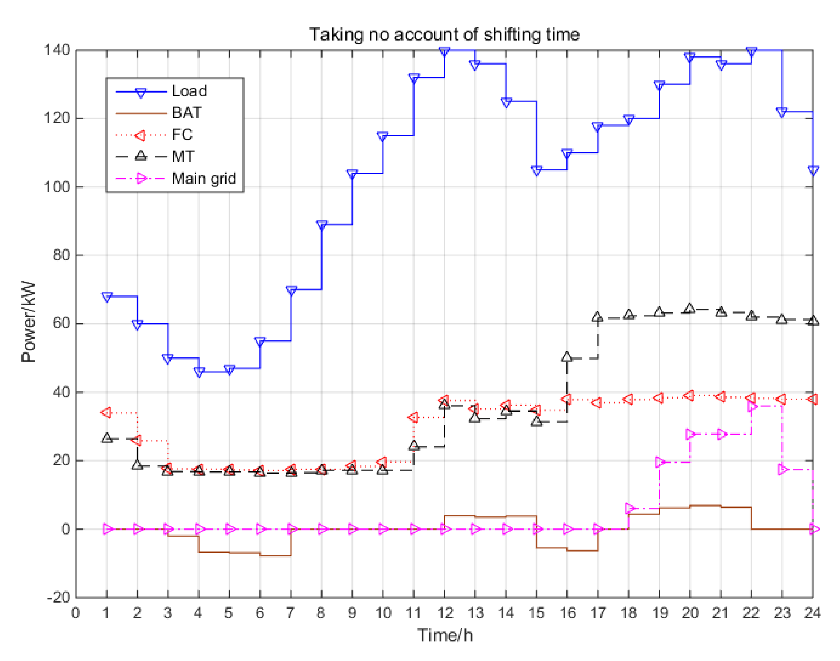
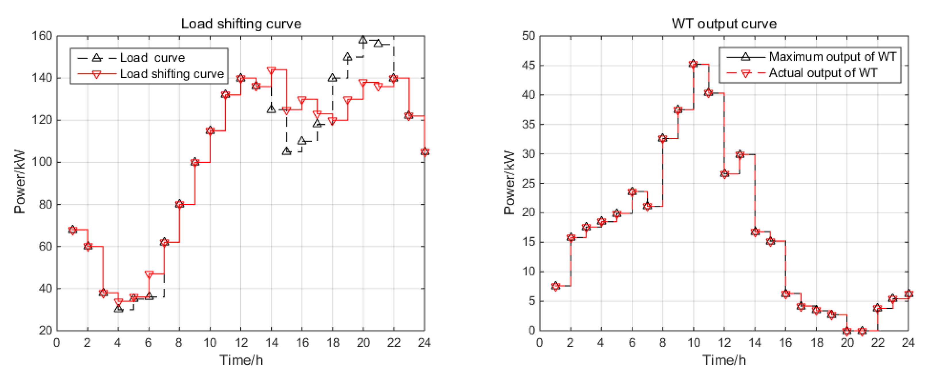
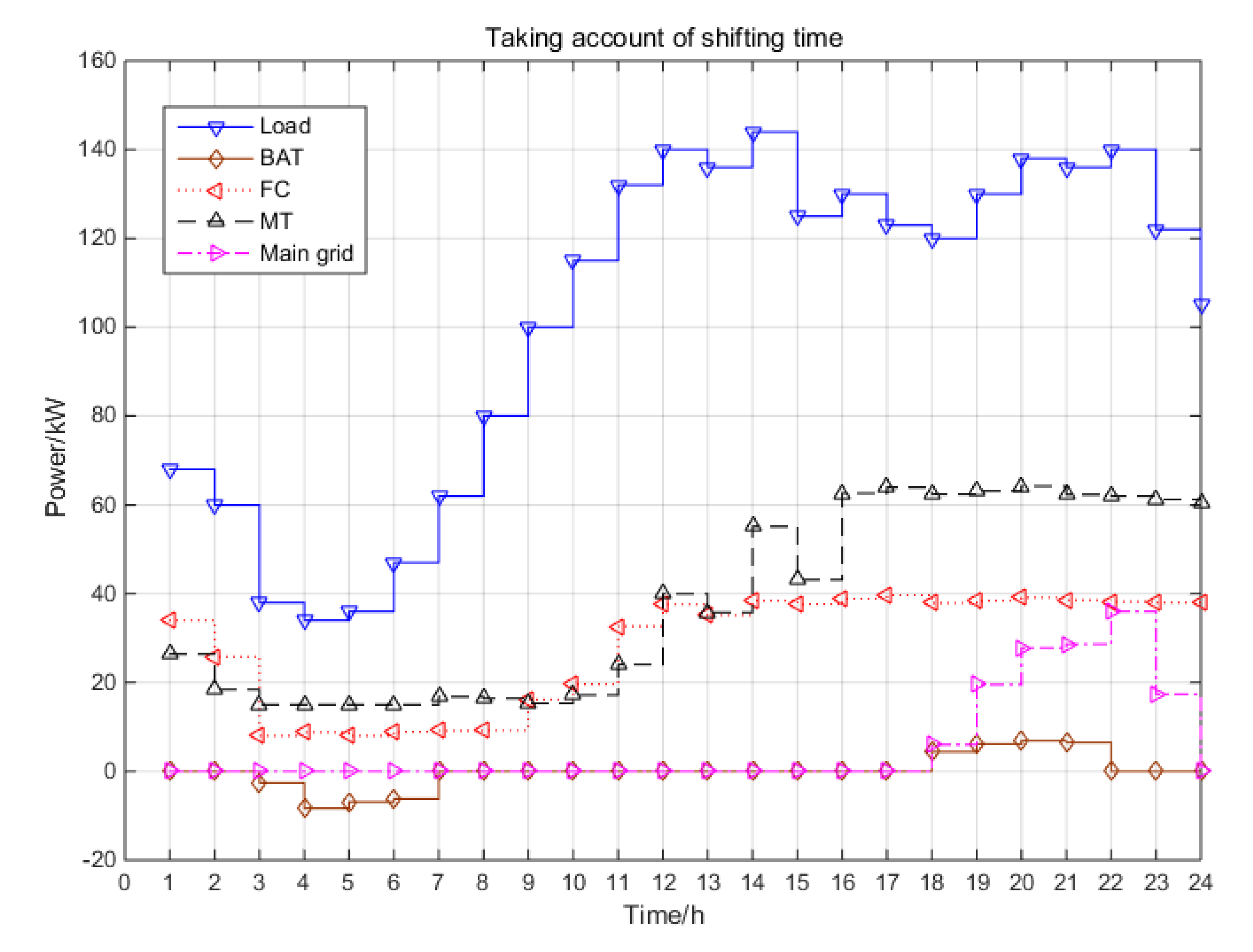
4. Simulation Results and Discussion

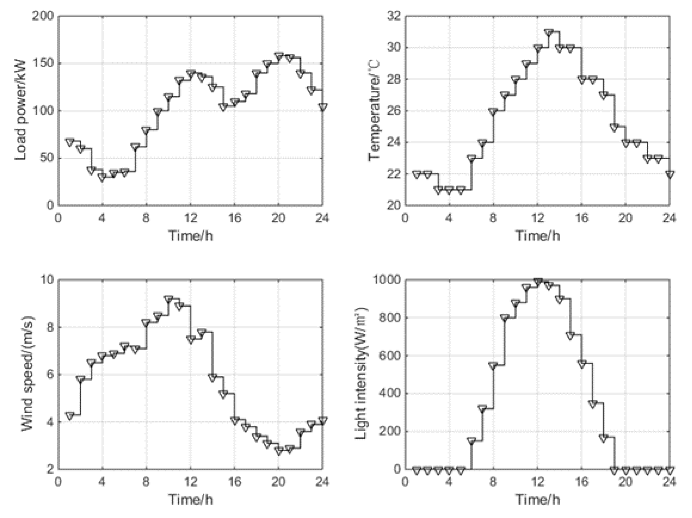
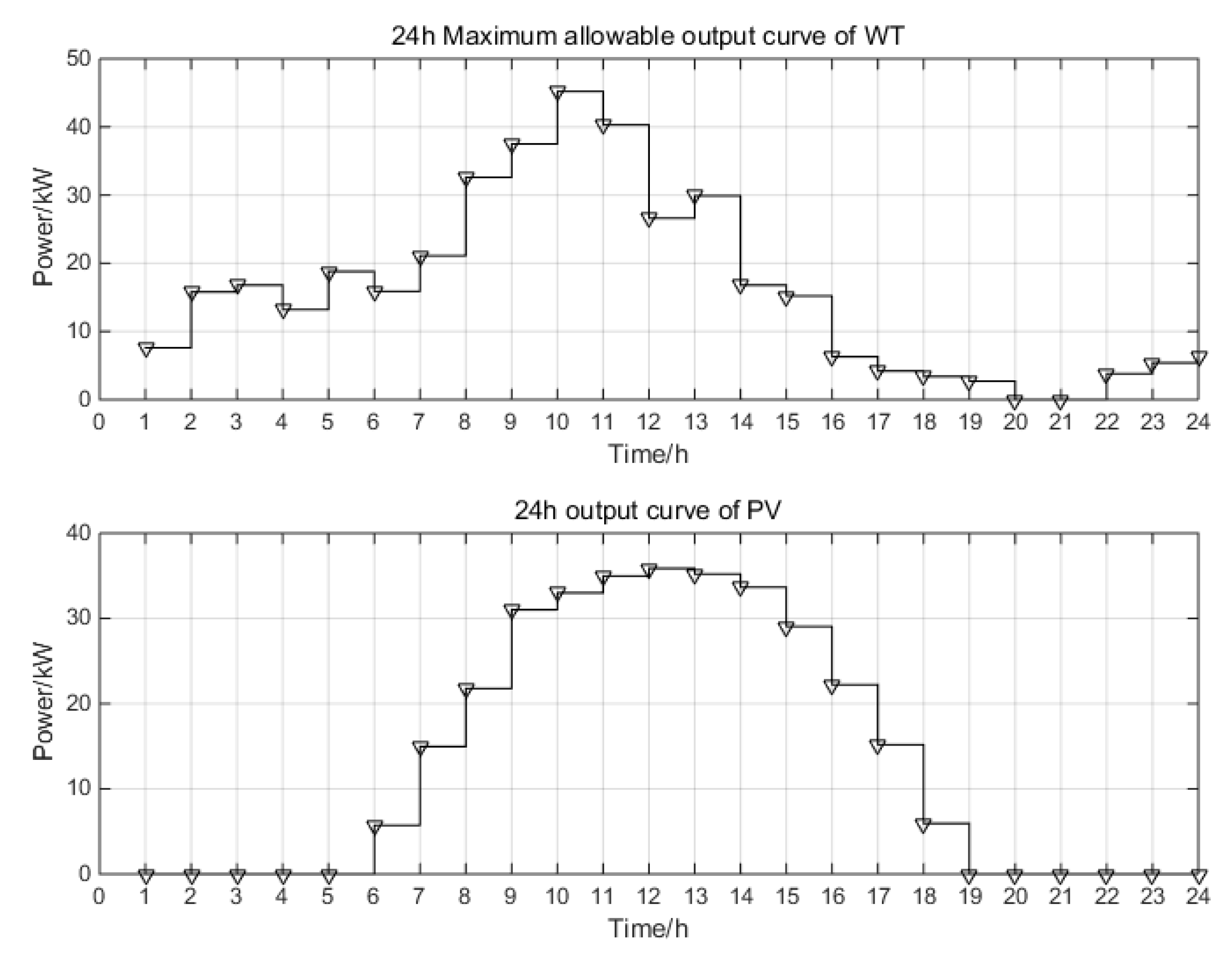
4.1. Calculation Parameters and Power Data Settings

By analyzing and discussing the operation of the microgrid under grid-connected mode to verify the authenticity and effectiveness of the model established above.

The improved biogeography-based optimization algorithm mentioned in this paper, which involves several units such as wind turbines, photovoltaic cells, micro gas turbines, batteries and interaction power with the main grid, is applied to the optimization of multiple objectives in the microgrid with hours as the time unit, the specific parameters are shown in

Table 1. Parameters of each Generators.

DG	Output Power/kW		Depreciable Life/a	Operation and Maintenance Coefficient (USD/kW·h)
	Pmax	Pmin
WT	50	0	10	0.0042
PV	40	0	20	0.0014
BAT	30	−30	10	0.0064
FC	40	8	10	0.0042
MT	65	14	10	0.0059

. Other parameters of the microgrid system include the maximum allowable charge capacity of the storage battery, which is 250 kWh; the maximum interaction power, which is 50 kw; to be specific, microgrid purchases electricity from the large grid as positive and sells it as negative. By investigating the local climate and electricity consumption and selecting a common summer weather, we learn that the peak power consumption of the day is at 12:00 and 20:00, and the maximum can reach 160 kW. In addition, other forecast data, such as light intensity, temperature and wind speed are given in Figure 1. It can be analyzed from Figure 1 that from 12:00 to 13:00 that day, the light intensity reached the maximum value of 1000 W/m², the temperature also reached the maximum value of 31℃, and the wind speed reached the maximum value of 9.2 m/s at 10:00. To ensure the maximum utilization of renewable energy and maximum economic and environmental benefits, wind turbines and photovoltaic cells will continue to run under the maximum power point trace mode (MPPT); the output curves are given in Figure 2. In one day, the output power of the wind turbine is the maximum at 10:00, and the photovoltaic power generation is the maximum at 12:00, and the values are 46 and 36 kW, respectively. From [12], we can know the real-time electricity price and pollution penalty standards and other electricity data. There are the following specific values of parameters in BBO and IBBO algorithms: the initial value of the population size NP is set to 100, and the maximum number of species S_max is also 100, upper limit of immigration rate and emigration rate I = E = 1.0, upper limit of mutation rate m_max = 0.005 and the number of iterations is limited to 500. Compared with the IBBO algorithm, the population size of the other algorithms is also set as 100, and the other parameter settings can be found in [10,11,22].

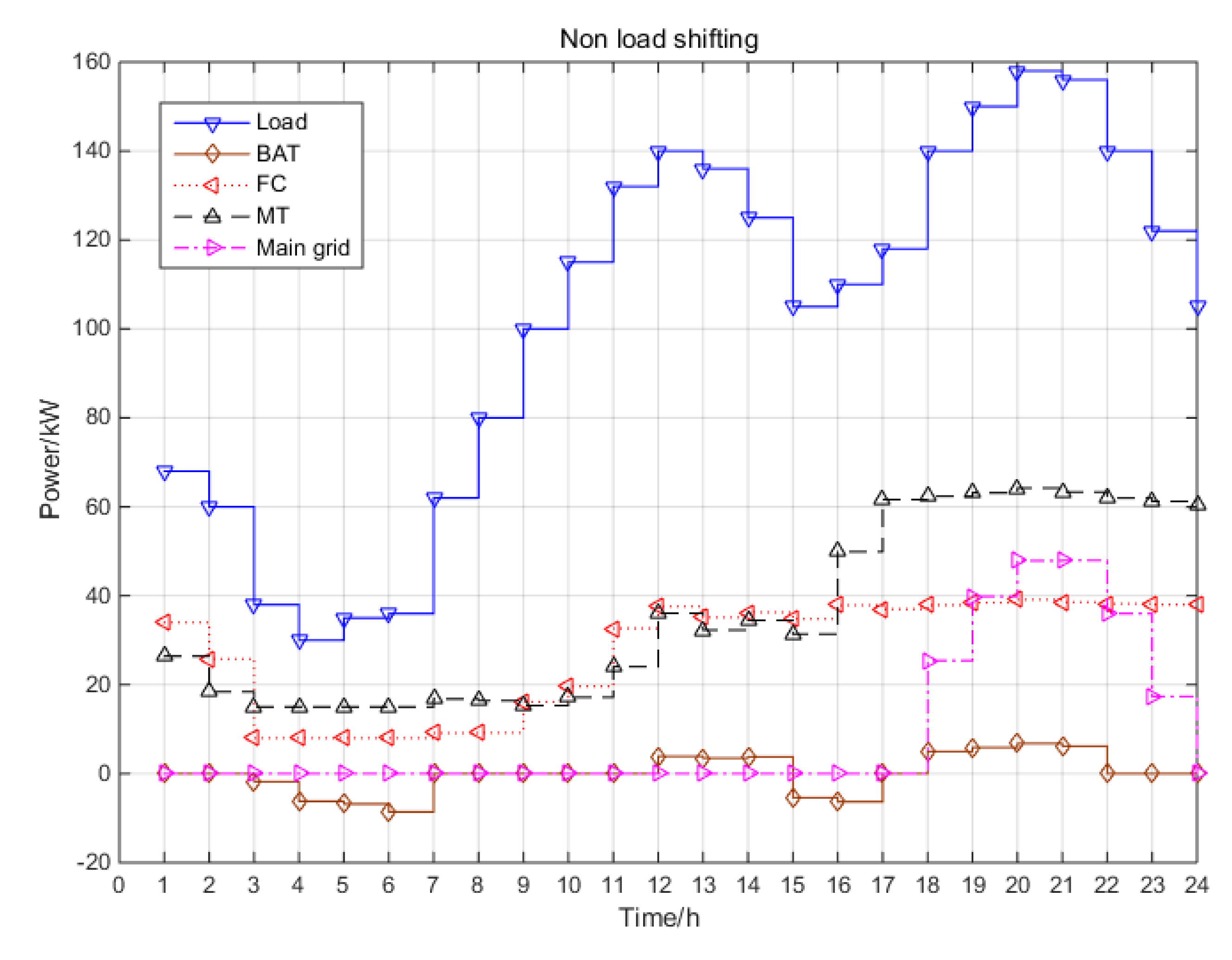
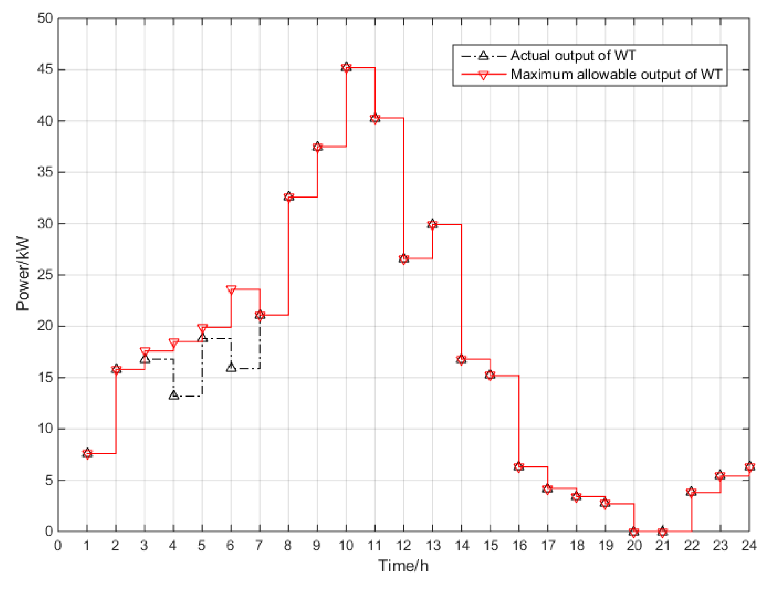
4.2. Simulation Results and Discussion

In order to verify the optimization ability of the IBBO algorithm, IBBO and basic BBO, as well as classic optimization algorithms PSO and GA [26], simulated the typical standard function [27] and compared the test results. The dimensions of each test function are all 30 dimensions, the maximum number of iterations is 1000, and the predetermined error of the function solution is 1.0 × 10⁻⁸. the representative and difficult-to-solve Ackley and Griewank functions can be taken as examples. The average value, standard deviation and the number of function evaluations and success rates obtained when the solution accuracy is reached are shown in

Table 2. Algorithm performance comparison.

Function	Algorithm	Average Value	Standard Deviation	Function Evaluation Times	Success Rate
Ackley	IBBO	1.1949 × 10−12	4.7684 × 10−23	140,640	100
	PSO	6.1748 × 10−3	3.2709 × 10−6	155,850	90
	GA	5.7820 × 10−2	3.6079 × 10−3	536,120	73.33
	BBO	7.1061 × 10−1	2.6396 × 10−1	1,329,270	23.33
Griewank	IBBO	7.3121 × 10−13	3.6763 × 10−27	124,320	100
	PSO	1.2079 × 10−4	3.8624 × 10−6	105,810	100
	GA	9.3740 × 10−2	5.0897 × 10−3	237,910	100
	BBO	6.4551 × 10−1	1.3315 × 10−2	—	0

. Among them, the success of the problem solving is defined as the algorithm’s convergence accuracy before the maximum function evaluation times reach a predetermined error, each algorithm runs independently 30 times and the maximum function evaluation times is 1.0 × 10⁶.

It can be seen from Table 2 that compared with the PSO, GA and basic BBO, the improved IBBO algorithm can achieve better convergence accuracy and stability. At the same time, the number of function evaluations used to achieve solution accuracy is also less. It shows that the IBBO algorithm has certain advantages in convergence accuracy, convergence speed and robustness compared with other algorithms, and has a good global search ability.

According to the dispatching strategy and the mathematical model built of the microgrid under the grid-connected mode, the operation state of the distributed generation for the typical summer microgrid is analyzed and solved using the IBBO algorithm. After optimized scheduling, the corresponding optimized output curve with non-load shifting of each micro power at each time is shown in Figure 3, and the comparison of the maximum allowable output and actual output power of WT is given in Figure 4.

In Figure 3, it is necessary to divide a day into several periods for analysis. The electricity valley time in the whole day is from 0:00 to 6:00, and its power demand can be as low as 30 kW; the electricity purchase cost to the main grid is relatively low. There is only weak light at 6:00 and PV provides hardly any output power, but there is wind power, and WT can continuously provide more than 20 kW of electric power. Due to the reasonable allocation of power resources, FC and MT operate at the lowest power, and the battery remains charged during the low power consumption period. Then, priority is given to purchasing electricity from the main grid to meet the load demand. Additionally, in combination with Figure 4, it can be seen that from 3:00 to 6:00, although the load power demand is met, the battery output power has been negative; therefore, the battery has been charging and due to its low power consumption and the capacity limitation of the battery, the actual output power of the WT is less than its maximum allowable output, resulting in a waste. After 7:00, the power consumption begins to increase gradually, and the light intensity gradually increases. From 7:00 to 10:00, the output of PV and WT combined with the low-power operation of FC and MT can basically meet the load power demand. From 10:00 to 14:00, with the gradual increase in power consumption, the output of WT and PV no longer meet the current load demand. Meanwhile, FC is almost close to full capacity, and MT also maintain the higher power operation. The battery is discharged during this period from 12:00 to 14:00, the peak time of electricity consumption. The local electricity valley time is from 15:00 to 16:00, which reaches the electricity valley bottom at 15:00. After the morning peak discharge, the battery is recharged during this period to store energy for the peak power consumption in the evening. After 17:00, the load demand begins to rise again, and at 20:00, the load reaches the peak of the whole day. Meanwhile, the light intensity gradually weakens, PV basically no longer has an output. From the wind speed forecast for the day, the wind speed is also currently low, although the power supply of WT is sustainable but very small. In this period, FC and MT operate at maximum power. Furthermore, the battery also discharges to meet the peak of power consumption. However, this period is the peak of the whole day, the total generation capacity of the microgrid is lower than the load demand; therefore, it is still necessary to purchase electricity from the main grid. After 23:00, the electricity consumption decreases, the FC and MT operate at reduced power, and the remaining capacity of the battery has also reached its lower limit.

Under the condition of PV and WT output all day, FC and MT are used to power generation with power purchase from the main grid to meet the all-day load demands. FC, O and M factors and environmental costs are significantly lower than MT due to a combination of economic and environmental costs, although FC also has higher fuel costs, but the comprehensive costs are significantly lower than MT. Therefore, in addition to the price of electricity valley time, FC is close to full load power generation, playing a major role. Meanwhile, the battery is charging in the low valley, while discharging in the peak, which reflects the value of cutting peaks and filling valleys and stabilizing fluctuation.

According to the proposed optimization scheduling model, the daily comprehensive operating cost calculated by IBBO is compared with BBO and the other two algorithms, and four algorithms are independently run 30 times to obtain the average value. The comparison results are shown in Figure 5.

It can be known from Figure 5, compared with IBFA, IPSO and BBO algorithms, that the IBBO algorithm has already converged in the 161st generation, and the convergence value of USD 204 is better than the other three algorithms; therefore, it can be concluded that the IBBO algorithm has great advantages in optimization accuracy, convergence speed and stability under the condition of the same population size and iteration times.

At the same time, the performance of the four algorithms in the calculation of the operating cost of the microgrid is evaluated. The comparison results are given in

Table 3. Comparison of optimization algorithms for calculating operating costs.

Optimization Method	Maximum Iteration Value/Times	Convergence Iterations/Times	Operating Costs/USD
IBFA	500	263	223
IPSO	500	212	218
BBO	500	275	212
IBBO	500	161	204

.

Obviously, in Table 3, the number of convergence iterations of the optimization algorithm proposed in this paper is significantly less than the other three algorithms. This is mainly due to the fact that the IBBO algorithm normalizes the individuals of each generation on the basis of the BBO algorithm and adds disturbance processing to the migration mechanism to speed up the optimization speed and reduce convergence iterations of the algorithm, which also makes it easier to obtain the optimal value of the operating cost from the IBBO algorithm.

Next, we consider the case where the interruptible load can perform power shifting in a microgrid operation. Suppose that the interruptible load can be power shifted, compared with the maximum power demand in the original period, the variation of the hourly power demand shifted $P_{LSm}$ is not more than 20 kW, and the total amount of shiftable power for the interruptible load $P_{LI}$ is not more than 80 kW in the whole day. Meanwhile, the effect of the shifting time quanta on the scheduling results does not need to be considered. The load shifting curve and the WT output curve without considering shifting time are given in Figure 6, and the optimization results of each micro-energy source is given in Figure 7.

From the load shifting curve in Figure 6, the peak load power of the whole day before the load shift reaches the maximum value of 160 kW from 18:00 to 21:00, which is also the period with low PV and WT power output and the period with the greatest amount of electricity purchased on that day. In addition, the load power valley drops to the minimum value of 30kW from 3:00 to 7:00. The power of interruptible load can be shifted to the low power consumption period of the whole day from 3:00 to 9:00, and the shift amount is the greatest from 3:00 to 6:00. After the load is shifted, the load power is cutting the peak and filling the valley, reducing the burden of power generation on the microgrid. As can be seen from the WT output curve in Figure 6 after power shifting, the maximum allowable output of WT is exactly in line with the actual output power, and there is no longer any wastage.

It can be seen from Figure 7 that FC and MT can operate at low power from 0:00 to 11:00, which can meet the load power demand with the power generation of PV and WT and recharge the batteries in the low power consumption period. After 12:00, the power generation of FC and MT increases gradually, and the power is close to full output during the peak period in the evening. Although there is still a need to purchase power from the main grid from 19:00 to 23:00 due to the lack of power generation in the microgrid, the power purchase has been significantly reduced compared to the operation of the uninterruptible load, i.e., Figure 3.

Then, we consider the case that power shifting can be performed, and the shifting time needs to be considered. With the other conditions remaining unchanged, suppose that the effect of the shifting time quanta on optimal scheduling needs to be considered, the load shifting curve and the WT output curve are given by Figure 8 and Figure 9, and the corresponding optimal output of each micro power supply is indicated.

Since the effect of the shifting time of interruptible load on the comprehensive evaluation is considered, the comparison of the load shifting curves between Figure 8 and Figure 6 shows that the shiftable power from 18:00 to 21:00 in Figure 6 is mainly shifted toward the morning period of the low power consumption of the whole day. Whereas only a fraction of the power is shifted to the period from 4:00 to 6:00 in Figure 8, most of the remaining power is shifted to the period from 14:00 to 17:00. There are two main reasons. Firstly, although the interruptible load is shifted from the evening peak period to the period between 4:00–6:00, which has a higher time cost in terms of shifting, the comprehensive cost is low because there is a situation where the WT power is abandoned during this period, resulting in the wasted part of this power being basically cost-free with only a time cost. Secondly, 13:00–17:00 is a local valley period in the whole day and shifting the evening peak power consumption to this period only increases the output power of FC and MT, because WT and PV are always outputting power during this time period, the load power demand after the shifting of microgrid can be met and the time cost of power shifting is low.

As can be seen from the comparison between Figure 9 and Figure 7, due to the shift of interruptible load in the evening peak, the period of local low power consumption, which originally occurred from 15:00 to 16:00, no longer exists. The battery is only charged during the valley period from 3:00 to 6:00, and it discharges in the evening peak period, in order to meet the shifting load demand, the output power of the fuel cell is increased, while the number of battery charge and discharge cycles is reduced, and the charge and discharge loss of the battery is reduced, thereby reducing the overall operating cost.

Comparing the above cases without considering load shifting and considering load shifting, the comprehensive operation cost including economic cost and environmental cost is calculated in

Table 4. Cost of non-load shifting and load shifting.

Scenario	Case	Comprehensive Operating Cost/USD
1	Non-load shifting	204.06
2	Taking no account of shifting time	190.34
3	Taking account of shifting time	195.46

.

In Table 4, the optimal comprehensive operating costs without considering interruptible load and considering interruptible load are given, respectively. Without considering interruptible load, the comprehensive operating cost is 204 US dollars, which is the highest among the three scheduling scenarios. When interruptible load is considered, the power generation of PV and WT is no longer wasted due to power shifting, and the coordinated generation of FC and MT has also changed; therefore, the comprehensive operating cost can be relatively reduced. Comparing scenarios two and three, in scenario two, the interruptible load shifts to the place where the power of the whole day is lower due to not considering the effect of the shifting time, and the scheduling scheme of the optimal comprehensive cost by meeting the conditions is given. In contrast, in scenario three, the inclusion of the shifting time causes the interruptible load to shift to the time with lower power, which is closer to the original operation time, and the comprehensive operating cost of scheme three is slightly higher than that in scenario two, but lower than that in scenario one.

Consequently, in microgrid operation, for the presence of the power shifting of interruptible load, considering the effect of environmental benefits and economic costs, and to ensure that the capacity constraints of the battery are met, we can conclude that the comprehensive operating cost after shifting interruptible load can be lower, and the time factor $\alpha$ in this paper is proposed to adjust the relationship between the power shifting time and the user acceptability. From the comparative results, on the user side, adopting reasonable load management schemes and power demand incentive measures can effectively improve the utilization rate of renewable energy and ensure the economy and effectiveness of the microgrid system operation.

5. Conclusions

This paper proposes a multi-objective optimal dispatching model of distributed power generation in the microgrid grid-connected mode that combines operating costs and environmental benefits. Meanwhile, on the user side, the power shifting for interruptible load is joined considering the effect of interruptible load on the operating cost of a microgrid based on battery storage capacity. Based on the proposed IBBO algorithm, a typical microgrid, as an example, containing a fuel cell, micro turbine, wind, storage battery, light and load is used to optimize the output of each distributed generator to achieve the maximum economic and environmental benefits, and the results obtained by comparing and analyzing another three optimization algorithms prove the superiority of the IBBO algorithm. Moreover, the optimization performance of BBO is improved by better designing the migration strategy and the determination principle of migration rate, and the reliability and applicability of the proposed model and algorithm are verified. This optimization operation method based on an improved biogeographical optimization algorithm can improve the level of microgrid operation technology. If we can properly consider the power shifting of interruptible load, effectively formulate the incentive measures for the user side, improve the management of the demand side and guide the load effectively, the maximum utilization of renewable energy can be achieved effectively, which is of certain significance to the maximization of the operation benefits of the microgrid.

References

1. Chen, J.J.; Qi, B.X.; Rong, Z.K.; Peng, K.; Zhao, Y.L.; Zhang, X.H. Multi-energy coordinated microgrid scheduling with integrated demand response for flexibility improvement. Energy 2020, 217, 119387. [Google Scholar] [CrossRef]
2. Kiptooa, M.K.; Lotfy, M.E.; Adewuyi, O.B.; Conteh, A.; Howlader, A.M.; Senjyu, T. Integrated approach for optimal techno-economic planning for high renewable energy-based isolated microgrid considering cost of energy storage and demand response strategies. Energy Convers. Manag. 2020, 215, 112917. [Google Scholar] [CrossRef]
3. Yong, L.; Zou, Y.; Tan, Y.; Cao, Y.; Liu, X.; Shahidepour, M.; Tian, S.; Bu, F. Optimal Stochastic Operation of Integrated Low-Carbon Electric Power, Natural Gas, and Heat Delivery System. IEEE Trans. Sustain. Energy 2018, 9, 273–283. [Google Scholar]
4. Samy, M.M.; Barakata, S.; Ramadan, H.S. Techno-economic analysis for rustic electrification in Egypt using multi-source renewable energy based on PV/wind/FC. Int. J. Hydrogen Energy 2020, 45, 11471–11483. [Google Scholar] [CrossRef]
5. Tanmay, D.; Ranjit, R.; Krishna, M.K. Impact of the penetration of distributed generation on optimal reactive power dispatch. Prot. Control Mod. Power Syst. 2020, 5, 2–26. [Google Scholar]
6. Takano, H.; Goto, R.; Hayashi, R.; Asano, H. Optimization Method for Operation Schedule of Microgrids Considering Uncertainty in Available Data. Energies 2021, 14, 2487. [Google Scholar] [CrossRef]
7. Lingmin, C.; Jiekang, W.; Fan, W.; Huiling, T.; Chanjie, L.; Yan, X. Energy flow optimization method for multi-energy system oriented tocombined cooling, heating and power. Energy 2020, 211, 118536. [Google Scholar] [CrossRef]
8. Tantrapon, K.; Jirapong, P.; Thararak, P. Mitigating microgrid voltage fluctuation using battery energy storage system with improved particle swarm optimization. Energy Rep. 2020, 6, 724–730. [Google Scholar] [CrossRef]
9. Nemati, M.; Braun, M.; Tenbohlen, S. Optimization of unit commitment and economic dispatch in microgrids based on genetic algorithm and mixed integer linear programming. Appl. Energy 2018, 210, 944–963. [Google Scholar] [CrossRef]
10. Nagapurkar, P.; Smith, J.D. Techno-economic optimization and environmental Life Cycle Assessment (LCA) of microgrids located in the US using genetic algorithm. Energy Convers. Manag. 2019, 181, 272–291. [Google Scholar] [CrossRef]
11. Roy, K.; Mandal, K.K.; Mandal, A.C.; Patra, S.N. Analysis of energy management in micro grid—A hybrid BFOA and ANN approach. Renew. Sustain. Energy Rev. 2018, 82, 4296–4308. [Google Scholar] [CrossRef]
12. Cunbin, L.; Jianye, Z.; Peng, L. Multi-objective Optimization Model of Micro-grid Operation Considering Cost, Pollution Discharge and Risk. Proc. CSEE 2014, 34, 3073–3079. [Google Scholar]
13. Chen, J.; Yang, X.; Zhu, L.; Zhang, M.; Li, Z. Microgrid multi-objective economic dispatch optimization. Proc. CSEE 2013, 33, 57–66. (In Chinese) [Google Scholar]
14. Chen, D.; Gong, Q.; Zhang, M.; Liu, D.; Du, L.; Shao, Q. Multi-objective optimal dispatch in wind power integrated system incorporating energy-environmental efficiency. Proc. CSEE 2011, 31, 10–17. (In Chinese) [Google Scholar]
15. Zhao, L.; Ju, G.; Lü, J. An improved genetic algorithm in multi-objective optimization and its application. Proc. CSEE 2008, 28, 96–102. (In Chinese) [Google Scholar]
16. Faisal, A.; Mohamed, H.; Koivo, N. Online management of microgrid with battery storage using multi-objective optimization. In Proceedings of the International Conference on Power Engineering, Energy and Electrical Drives, Setubal, Portugal, 12–14 April 2007; pp. 231–236. [Google Scholar]
17. Ma, X.; Wu, Y.; Fang, H.; Sun, Y. Optimal sizing of hybrid solar-wind distributed generation in an island micro grid using improved bacterial foraging algorithm. Proc. CSEE 2011, 31, 17–25. [Google Scholar]
18. Li, P.; Xu, W.; Zhou, Z.; Li, R. Optimal Operation of Microgrid Based on Improved Gravitational Search Algorithm. Proc. CSEE 2014, 34, 3073–3079. [Google Scholar]
19. Zheng, Z.; Ai, Q.; Xu, W.; Shi, J.; Xie, D.; Han, L. A multi-objective dispatch optimization strategy for economic operation of smart grids. Power Syst. Technol. 2010, 34, 7–13. (In Chinese) [Google Scholar]
20. Liu, D.; Guo, J.; Huang, Y.; Wang, W. Dynamic economic dispatch of wind integrated power system based on wind power probabilistic forecasting and operation risk constraints. Proc. CSEE 2013, 33, 9–15. (In Chinese) [Google Scholar]
21. Mohammadi, S.; Mozafari, B.; Solimani, S.; Niknam, T. An adaptive modified firefly optimization algorithm based on Hong’s Point Estimate Method to optimal operation management in a microgrid with consideration of uncertainties. Energy 2013, 51, 339–348. [Google Scholar] [CrossRef]
22. Simon, D. Biogeography-based optimization. IEEE Trans. Evol. Comput. 2008, 12, 702–713. [Google Scholar] [CrossRef] [Green Version]
23. Khurmi, R.S.; Sedha, R.S. Materials Science. S. Chand. 2008. Available online: https://refhub.elsevier.com/S0360-3199(18)31672-0/sref36 (accessed on 2 September 2021).
24. Giovanni, C.; Luca, M. Resolution of Spike Overlapping by Biogeography-Based Optimization. Electronics 2021, 10, 1469. [Google Scholar]
25. Khosravi, K.; Bordbar, M.; Paryani, S.; Saco, P.M.; Kazakis, N. New hybrid-based approach for improving the accuracy of coastal aquifer vulnerability assessment maps. Sci. Total Environ. 2021, 767, 145416. [Google Scholar] [CrossRef]
26. Holland, J.H. Adaptation in Natural and Artificial Systems: An Introductory Analysis with Applications to Biology, Control, and Artificial Intelligence, 2nd ed.; MIT Press: Cambridge, MA, USA, 1992. [Google Scholar]
27. Rahnamayan, S.; Tizhoosh, H.R.; Salama, M.M.A. Opposition-based differential evolution. IEEE Trans. Evolut. Comput. 2008, 12, 64–79. [Google Scholar] [CrossRef] [Green Version]
Figure 1. Predicted value of load power, wind speed, temperature and light intensity.
Symmetry 13 01707 g001
Figure 2. Predicted the output of WT and PV in a day.
Symmetry 13 01707 g002
Figure 3. The comprehensive optimal scheduling results with non−load shifting.
Symmetry 13 01707 g003
Figure 4. Comparison of the maximum output and actual output of WT.
Symmetry 13 01707 g004
Figure 5. Comprehensive cost by 4 algorithms.
Symmetry 13 01707 g005
Figure 6. Output curves of the load shifting and WT while taking no account of shifting time.
Symmetry 13 01707 g006
Figure 7. Results of the comprehensive optimal scheduling while taking no account of shifting time.
Symmetry 13 01707 g007
Figure 8. Output curves of the load shifting and WT while taking account of shifting time.
Symmetry 13 01707 g008
Figure 9. Results of the comprehensive optimal scheduling while taking account of shifting time.
Symmetry 13 01707 g009