Short-Term Energy Forecasting Using Machine-Learning-Based Ensemble Voting Regression

Abstract

Meeting the required amount of energy between supply and demand is indispensable for energy manufacturers. Accordingly, electric industries have paid attention to short-term energy forecasting to assist their management system. This paper firstly compares multiple machine learning (ML) regressors during the training process. Five best ML algorithms, such as extra trees regressor (ETR), random forest regressor (RFR), light gradient boosting machine (LGBM), gradient boosting regressor (GBR), and K neighbors regressor (KNN) are trained to build our proposed voting regressor (VR) model. Final predictions are performed using the proposed ensemble VR and compared with five selected ML benchmark models. Statistical autoregressive moving average (ARIMA) is also compared with the proposed model to reveal results. For the experiments, usage energy and weather data are gathered from four regions of Jeju Island. Error measurements, including mean absolute percentage error (MAPE), mean absolute error (MAE), and mean squared error (MSE) are computed to evaluate the forecasting performance. Our proposed model outperforms six baseline models in terms of the result comparison, giving a minimum MAPE of 0.845% on the whole test set. This improved performance shows that our approach is promising for symmetrical forecasting using time series energy data in the power system sector.

1. Introduction

The energy sector is one of the influential factors affecting the economic development of a country. The economy might go down if there is not sufficient energy to provide to the end users [1]. Therefore, energy industries have to produce enough energy by balancing supply and consumption, making energy forecasting essential in the energy management system. Moreover, it also helps reduce operating and generating costs and conduct short-term scheduling functions in the power system. Forecasting can be divided into three terms based on predictive duration: short term, medium term, and long term [2]. This research mainly focuses on short-term energy forecasting because it considers next-hour prediction using hourly energy data.

Research on short-term energy forecasting has been conducted using different models that classify statistical time series and ML models. Autoregressive (AR), moving average (MA), autoregressive moving average (ARMA), etc., are included in the first group [3]. These models are beneficial for non-real-time forecasting, but they cannot handle nonlinear load consumption. Thus, ML algorithms have been widely used in forecasting to overcome nonlinear problems in energy data. They can be split into two groups: regression analysis and neural-network-based models. Many ML regressors such as decision trees regressors, boosting regressors, and bagging regressors have been investigated [4]. Among them, tree-based regressors such as extra trees regressor (ETR) [5], random forest regressor (RFR) [6], and classification and regression tree (CART) [7] have been commonly applied in energy forecasting because of their simple tree structure and easy understanding.

The random forest (RF) algorithm, proposed by Leo Breiman, is one of the ML algorithms that can predict a large amount of data [8]. The four main processes of the RF algorithm are bootstrap resampling, random feature selection, out-of-bag (OOB) error estimation, and a fully grown decision tree [9]. This algorithm generates multiple decision trees (so-called weak learners) from the given training samples. Each tree’s exact number of samples is randomly chosen to form a new training sample using bootstrap resampling. The unselected samples are defined as out-of-bag samples during the training process. Afterward, the RF tree is grown entirely using the selected new training sample without pruning. Unlike the CART, the RF determines only a small number of features randomly instead of all predictor features. After training multiple times, the decision trees are then created randomly as a forest. The RF algorithm estimates the OOB error during the forest construction instead of using cross-validation like other tree-based models. Finally, it collects predictions from all weak learners and combines them using the bagging ensemble method to perform the final predictions. Lahouar et al. conducted a day-ahead load forecasting using the RF technique [10]. Their research highlighted that the RF was flexible with expert selection, load profiles, and complex customer behaviors and proved to have better performance in all season and calendar effects. Dudek also investigated the RF algorithm, combining regression trees with only a few parameters for short-term load forecasting (STLF). His research also revealed that the RF had the benefit of eliminating nonstationarity and filtering trends and seasonal cycles longer than the daily cycle [11].

The ETR algorithm, also known as extremely randomized trees, was proposed by Geurts et al. [5]. It is also related to the class of tree-based ensemble methods for implementing classification and regression tasks. The ETR algorithm extends the randomization of the RF algorithm. ETR uses all the training samples to train each ensemble member, while RF uses the tree-bagging step to generate a training subset for each tree. When splitting the tree, ETR randomly selects the best feature and its corresponding value to reduce overfitting and obtain better performance than RFR [12]. Gabriel analyzed electric load forecasts using ETR, XGBoost, and statistical time series models. In their research, ETR provided the best forecasting performance over traditional time series methods in the case of lengthier historical load data [13]. Alawadi et al. also proved that the increment in forecasting time does not affect the accuracy of ETR after comparing it with multiple ML algorithms on indoor temperature forecasting, considering user comfort levels, and reducing energy consumption [14].

Among the most prominent ensemble ML algorithms, gradient boosting machine (GBM) algorithms are also popular because of their high flexibility and interpretability achieved by transforming weak learners into strong learners. In the case of regression or classification, their procedures involve multiple weak learners trained sequentially by reweighting the original training data. The final prediction is performed using a weighted majority vote of sequentially trained learners. Friedman proposed a statistical view of boosting as an additive logistic regression model in the early 20th century [15]. Subsequently, it was extended as the estimation of a function by optimizing a loss criterion via a steepest gradient descent in the function space [16,17]. Some recent boosting variants such as extreme gradient boosting (XGBoost) [18], light gradient boosting machine (LGBM) [19], and categorical boosting (CatBoost) [20] have been developed by focusing on the increment of speed and predictive performance, and achieved robustness results in real applications and forecasting competitions. In recent years, boosting-tree-based algorithms have been widely applied in many areas, namely, computer vision [21], biology [22], chemistry [23], energy [24], etc. In particular, boosting has provided great advances in the energy sector in terms of highest predictive performance [25,26,27].

Fix and Hodges first introduced the nearest neighbor method as nonparametric classification, one of the most straightforward techniques in predictive mining [28]. This method provides the actual regression function without making strong assumptions for the estimation. It is easily understandable as kernel and nearest neighbors regression estimators are local univariate estimators. The K-nearest neighbors (KNN) algorithm was proposed to find K training samples closest to the target in the training set [29]. The most relative K value is chosen based on the nearest distance to classify the input features. The majority of K-nearest neighbors then gather a similar group of the specific input training set. Therefore, the KNN algorithm mainly depends on the distance and voting function of the selected optimal value of K. Fan et al. applied the KNN algorithm to classify Chinese load patterns to improve the accuracy of STLF [30]. In their research, the Euclidean distance function was used as the weight of KNN for a better load classification. Moreover, the KNN algorithm was utilized to classify and predict hourly energy consumption data in the work of Wahid and Kim. They revealed the effectiveness of the KNN algorithm by observing hyperparameters [31].

It is hard to make a reliable prediction of the decision-making process in the energy sector because of asymmetric information. The proper forecasting method with symmetric errors must be selected to obtain better predictions to overcome this. Accordingly, in this paper, seventeen ML were trained and their forecasting performances compared using error measurements. After comparing seventeen ML algorithms, this research aimed to fit a voting regressor, which combined the five best ML models, including ETR, RFR, LGBM, GBM, and KNN. We included meteorological data to train all ML algorithms, including temperature, humidity, wind speed, etc. These features primarily affect energy consumption due to seasonal effects along with meterological conditions. Our ensemble proposed model could improve forecasting error using the five best ML models.

1.1. Contribution

The highlighted contributions of this research are as follows:

1.

A forecasting performance comparison of seventeen ML algorithms on a training set using error metrics was conducted during the training process.

2.

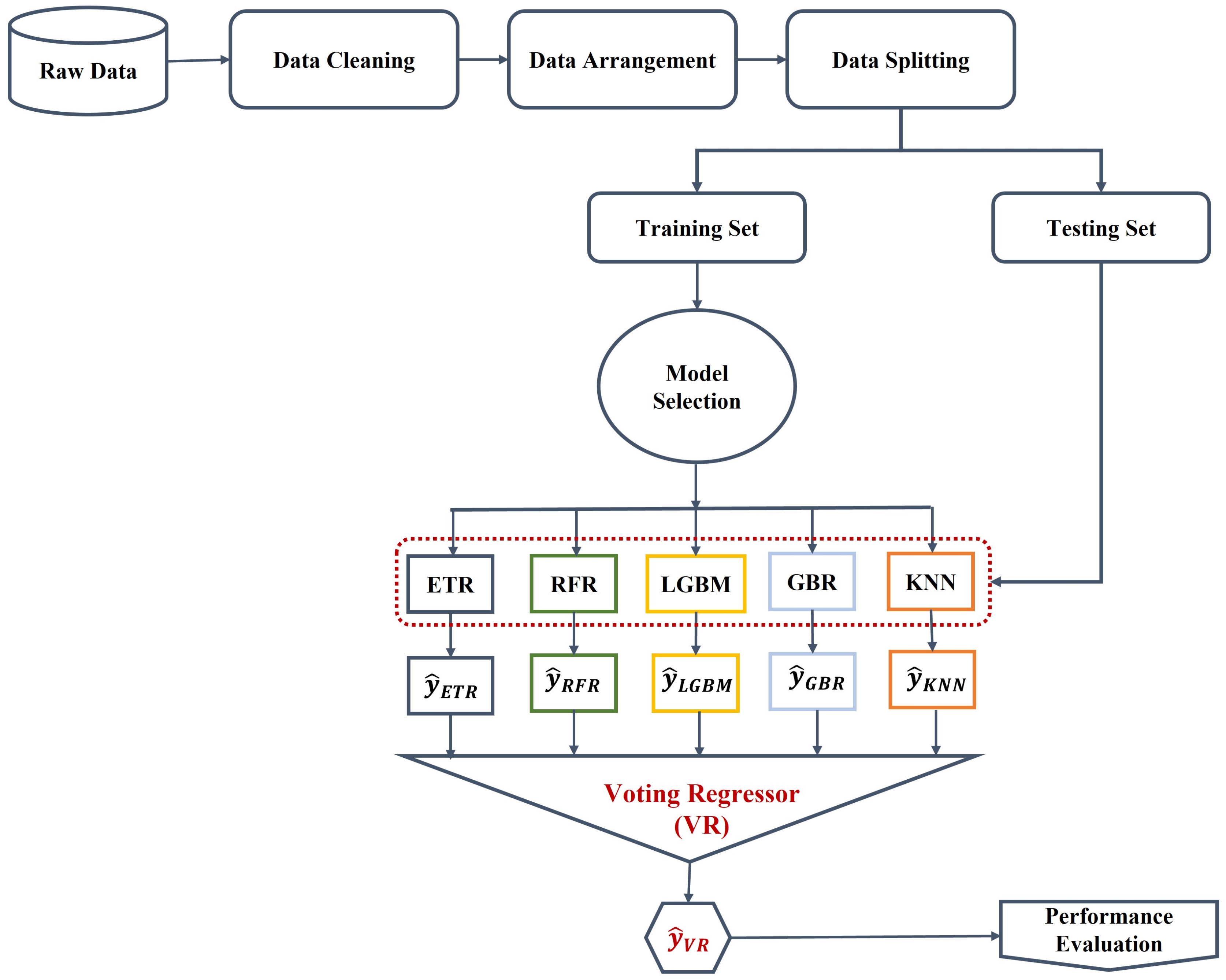
The top five ML algorithms, namely ETR, RFR, LGBM, GBR, and KNN, that had minimum errors were selected and combined to build the proposed VR algorithm.

3.

To conduct final predictions and improve accuracy, our ensemble VR model performed a majority voting and selected the best predictions among the five ML algorithms.

4.

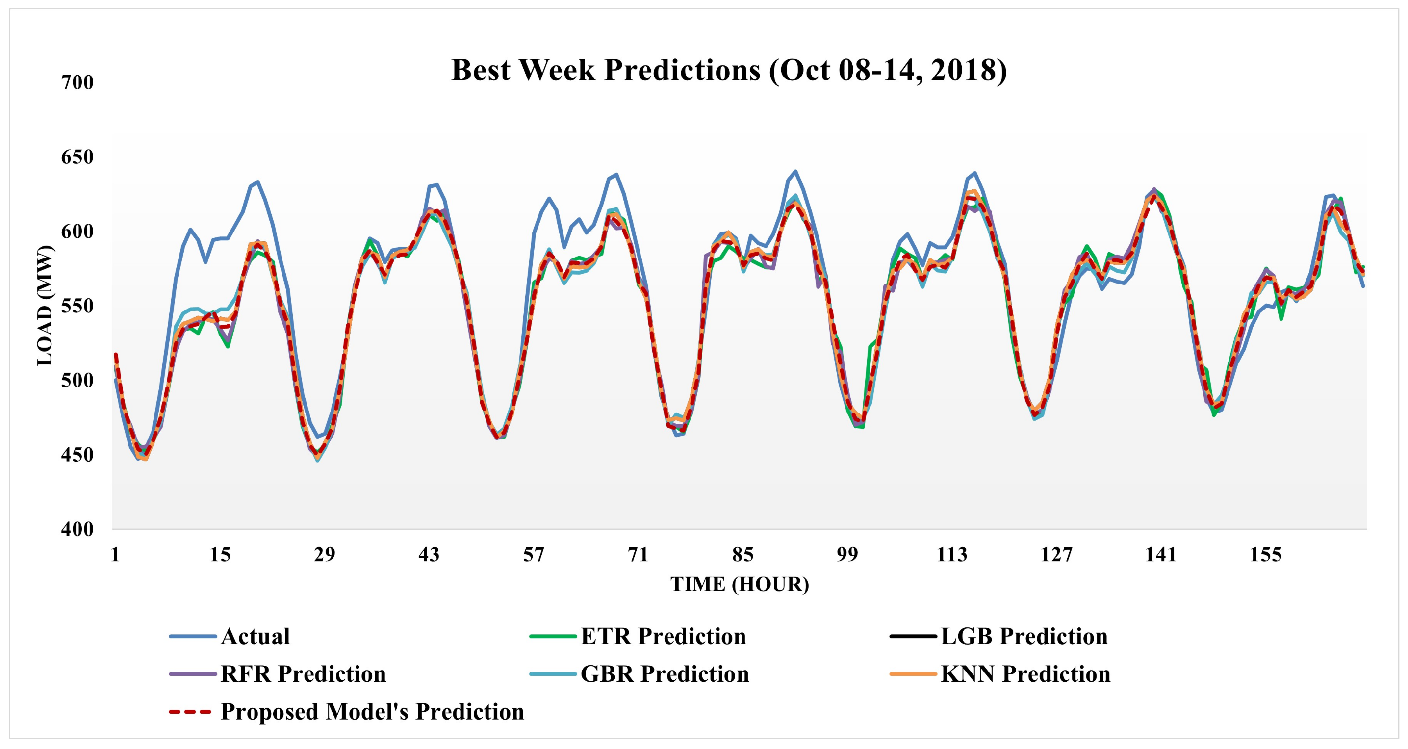
The performance evaluation was finally conducted by comparing the proposed model and the five standalone ML and ARIMA models.

1.2. Paper Structure

The arrangement of this paper is described as follows. Existing researches on energy forecasting using different forecasting models are reviewed in Section 2. In Section 3, the primary proposed system is presented, which involves information about data collection, data analysis, input selection, and system modeling. Generated results of all models are discussed and compared in Section 4. The conclusion of this paper takes place in Section 5.

2. Prior Works

In recent years, ML algorithms have been commonly used in many research areas to lessen the workload. For instance, the GBM model has been proposed in many applications using different data such as image processing, bilogical data, chemical data, energy data [21,22,23,24]. In the study of Wu et al., the GBM-based multiple kernel learning (MKL) was proposed with the extension of transfer learning algorithms, including antagonistic, homogeneous, and heterogeneous. Their proposed framework on STLF provided better results than baseline models [32]. During the global energy forecasting competition 2012, Lloyd also applied the GBM algorithm and Gaussian process regression with three different kernel functions that were proven very effective for predictive modeling and load forecasting [33]. In the work of Friedrich and Afshari, the transfer function model was applied using load data from Abu Dhabi for one-day and two-day forecasting, and results were compared with autoregressive integrated moving average (ARIMA) and artificial neural network (ANN) [34].

The principles of similar pattern-based methods affecting short-term load forecasting (STLF) were presented by Dudek. Afterward, similar pattern-based local linear regression models were proposed using Polish power system data for STLF. His proposed stepwise and lasso regressors outperformed other benchmark models: ARIMA, ANN, exponential smoothing, and Nadaraya–Watson estimator [35,36,37]. For load forecasting, KNN and support vector machine (SVM) methods were implemented, whereas the feature selection was conducted by a DT regression and recursive feature elimination (RFE) [38]. Even though these above-mentioned ML standalone algorithms provide good results for energy forecasting, some algorithms often can not handle complex nonlinear relationships and have computational efficiency. Considering the weakness of ML algorithms, hybridizing two or more advanced algorithms can be considered to generate reliable forecasts by enhancing their performance.

The ensemble method based on two ML algorithms, such as variational mode decomposition (VMD) and extreme learning machine (ELM) was proposed for multi-step ahead load forecasting. This proposed model was optimized by differential evolution algorithms using two electric load series [39]. Likewise, the combination of DT and SVM using smart meter data was proposed for one-week test predictions by Zhang et al. and obtained better forecasting performance [40]. Jihoon et al. also performed a hybrid method that combined RFR and multilayer perceptron (MLP) using power consumption data to predict one week ahead. Better forecasting accuracy was obtained by using their hybrid model over standalone forecasting ML models [41]. The ensemble model including cat-boost (CB), GBM, and MLP joined along with feature selection by genetic algorithm (GA) was conducted and compared with other ML baseline models in the work of Khan and Byun. Moreover, they also hybridized XGBoost, SVM regression, and KNN regressor algorithms. Their results showed that the ensemble approach could improve the forecasting accuracy [42].

In addition, some authors created ensembles in two ways, averaging and stacking, by combining SVM, RFR, and deep belief network (DBN) forecasting models in solar power forecasting [43]. The SVM model was used to generate forecasts, and these results were combined by using the RFR model for solar power forecasting in the cited work [44]. Similarly, three different ensemble methods, namely, linear, normal distribution, and normal distribution with additional features, using seven ML algorithms were proposed by Mohammed and Aung. Their proposed methods were compared and outperformed statistical models [45]. Tree-based ensemble methods such as RFR and ETR were applied to the prediction of photovoltaic generation output, and their predictive results were better than SVM [46]. According to the improved accuracy and the confidence level of the forecasts from the above-mentioned cited papers, combining two or more forecasting models is a noticeably better approach than applying single algorithms. Therefore, this paper also adopts an ensemble technique, which votes among five ML algorithms to improve the forecasting accuracy.

3. Proposed System

This section mainly presents a detailed explanation of our proposed system, including data collection, data analysis, input selection, and system modeling.

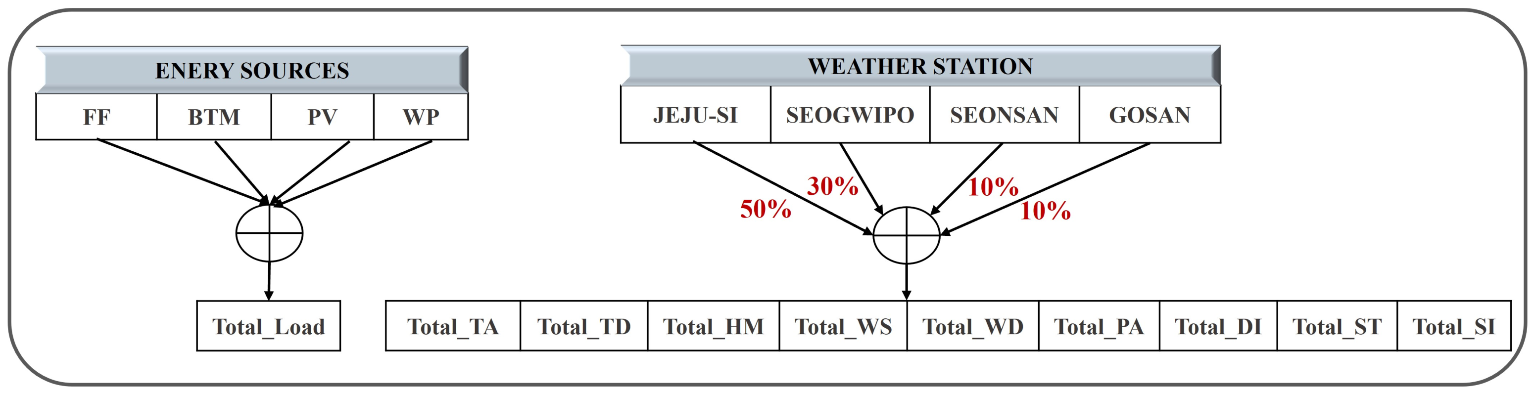
3.1. Data Collection

Our energy consumption data was collected from four primary energy sources such as fossil-fuel-based energy (FF), behind-the-meter (BTM), photovoltaic (PV), and wind power sources (WP). We denoted our actual energy data as Total_Load in MW, which were used for target variables. Jeju Island has four regions, the so-called JEJU-SI, SEOGWIPO, SEONSAN, and GOSAN. Each area has its own weather station that provides nine weather features. As we used Total_Load for the whole Jeju Island, we also aggregated all weather information by averaging the percentages of the whole island corresponding to each region. Accordingly, 50% of JEJU-SI, 30% of SEOGWIPO, 10% of SEONSAN, and 10% of GOSAN data were used. Therefore, nine weather features were considered: three temperature features, including the average temperature (Total_TA), the temperature of dew point (Total_TD), and the sensible temperature (Total_ST) measured in degree Celsius (${}^{\circ }$C), the humidity (Total_HM) in %, the wind speed (Total_WS) in m/s, the wind direction degree in degree (${}^{\circ }$), the atmospheric pressure on the ground (Total_PA) in hPa, the discomfort index (Total_DI), and the solar irradiation quantity (Total_SI) in (Mj/m${}^2$). The source information of collected load and weather data is described in Figure 1.

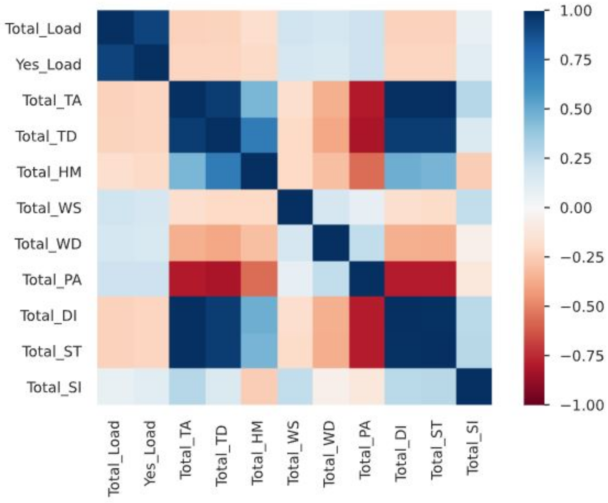
3.2. Data Analysis and Input Selection

The descriptive statistics for each variable are indicated in

Table 1. Descriptive statistics of input variables.

No	Variables	Min	Max	Mean	SD	CV	Unit
1	Total_Load	233	951	629.56	103.32	0.16	MW
2	Yes_Load	233	951	629.56	103.32	0.16	MW
3	Total_TA	−2.40	33.80	16.81	7.98	0.47	${}^{\circ }$C
4	Total_TD	−10.70	28.30	11.46	9.48	0.83	${}^{\circ }$C
5	Total_HM	21	99.20	72.33	14.67	0.20	%
6	Total_WS	0	22.40	3.04	1.46	0.48	m/s
7	Total_WD	0	360	190.55	84.52	0.44	${}^{\circ }$
8	Total_PA	704.30	1032.40	1011.90	11.68	0.01	hPa
9	Total_DI	30.10	86.50	61.97	12.35	0.20	-
10	Total_ST	−7.40	33.80	16.24	8.81	0.54	${}^{\circ }$C
11	Total_SI	0	2.40	0.32	0.54	1.67	Mj/m${}^2$

. As our target variable is Total_Load, we considered the load from yesterday (Yes_Load) as one of the independent variables. Consequently, there were ten input variables, including Yes_Load and nine weather variables, to forecast the next day’s load. The minimum (Min), maximum (Max), mean ($\mu$), standard deviation (SD), and coefficient of variation (CV) were calculated to see the extent of our variables. The mathematical expressions of $\mu$, SD, and CV are:

$$\mu =\sum x/n$$

(1)

$$SD=\sqrt{\sum {(x-\mu )}^2/(n-1)}$$

(2)

$$CV=SD/\mu$$

(3)

where x are the observations and n is the number of observations.

In terms of CV in Table 1, all input variables except Total_SI obtained CV values less than 1, meaning a low variance in the data. However, the last variable had a high variance, showing a 1.67 CV value. To better understand the data, the correlation coefficient ($\rho$) of Spearman was determined to catch nonlinear monotonic correlation between two variables, as represented in Figure 2. It indicates a value between −1 and +1 and assumes a negative $\rho$ is negatively correlated, while a positive one is positively correlated. There is no correlation between the two variables if the correlation coefficient is zero. Regarding the correlation diagram, Total_Load has a positive correlation with Yes_Load and vice versa. It is negatively correlated with Total_TA, Total_TD, Total_HM, Total_DI, and Total_ST, whereas there is close to zero correlation with Total_WS, Total_WD, Total_PA, and Total_SI. The Spearman’s rank correlation coefficient ($\rho$) can be formulated as follows:

$$\rho =1-(6\sum d_i^2)/n(n^2-1)$$

(4)

where $d_i$ is the difference between the two ranks of each observation and n is the number of observations.

3.3. System Modeling

The overall workflow of the proposed system is revealed in Figure 3. Initially, three-year raw data, including load and meteorological features, were loaded into the training process. Secondly, feature engineering involved data cleaning, data arrangement, and data splitting. In the process of data cleaning, we checked missing values and outliers in the raw data and then replaced outliers by moving averages. Cleaned data were then arranged according to ten independent variables and one target variable in order to train the ML algorithms. The next step consisted in splitting the arranged data into two sets, training and testing, based on predefined duration. The training data were provided to the training process of the model selection that was conducted using the so-called function compare_models from the PyCaret open source package. From this stage, seventeen ML models were generated from the training data, and error metrics among all models were compared. We then selected the five top ML algorithms with minimum errors and trained them to perform test predictions. Each single ML model performed predictions using one-year testing data. In Figure 3, ${\widehat{y}}_{ETR}$, ${\widehat{y}}_{RFR}$, ${\widehat{y}}_{LGBM}$, ${\widehat{y}}_{GBR}$, ${\widehat{y}}_{KNN}$ represent the predictions of each ML model. Afterward, these five algorithms were combined to build a voting regressor (VR) algorithm that voted the best predictor among them, to fit the final trained VR. Final predictions of the trained VR (${\widehat{y}}_{VR}$) on the testing set were executed. The evaluation of the proposed model was finally accomplished using error measurements. Five ML algorithms and the ARIMA model were compared with the proposed model with the purpose of a monthly result comparison.

The detailed error comparison of seventeen ML algorithms during the training process is indicated in

Table 2. Comparison of error metrics and computation time for all trained ML algorithms.

No	ML Algorithm	MAPE (%)	MAE ($\mathit{MW}$)	MSE (${\mathit{MW}}^2$)	Time (s)
1	Extra trees regressor (ETR)	3.10	19.37	726.74	2.79
2	Random forest regressor (RFR)	3.20	20.05	771.27	5.88
3	Light gradient boosting machine (LGBM)	3.40	20.88	808.37	0.40
4	Gradient boosting regressor (GBR)	3.70	22.71	947.63	1.40
5	K neighbors regressor (KNN)	4.00	25.06	1175.54	0.08
6	Bayesian ridge (BR)	4.20	25.77	1281.17	0.02
7	Linear regression (LR)	4.20	25.78	1281.17	0.16
8	Lasso regression (Lasso)	4.10	25.73	1286.85	0.03
9	Ridge regression (Ridge)	4.20	25.78	1281.17	0.02
10	Huber regressor (Huber)	4.10	25.44	1300.88	0.19
11	Elastic net (EN)	4.20	25.83	1305.45	0.03
12	Orthogonal matching pursuit (OMP)	4.30	27.07	1427.19	0.02
13	AdaBoost regressor (Ada)	5.20	30.61	1474.62	0.72
14	Decision tree regressor (DT)	4.40	27.26	1549.40	0.10
15	Least angle regression (LAR)	4.80	29.66	1648.04	0.02
16	Passive aggressive regressor (PAR)	6.60	41.37	2890.09	0.03
17	Lasso least angle regression (LLAR)	13.20	79.50	9831.52	0.02

. The computation time of each trained algorithm was also evaluated and is shown in the comparison table. The error performance on each algorithm was checked, and then we selected the top five algorithms with minimum errors among all. ETR, RFR, and LGBM models provide forecasting MAPEs of approximately 3% regardless of computing time. GBR and KNN have MAPEs of 3.7% and 4%, respectively. All the other ML models except Ada, PAR, and LLAR achieve MAPEs over 4% in energy forecasting. Ada and PAR obtain MAPE of about 5% and 6%, which can be considered acceptable performance. However, the LLAR algorithm is unsuitable for energy forecasting because it has the highest errors in all measurements.

During the training module, each trained forecasting model was fitted together with different parameters. Both ETR and RFR algorithms were trained with the number of trees in the forest (n_estimators = 100) and split criteria (MSE). Likewise, the LGBM and GBR algorithms used the same parameters and a 0.1 boosting learning rate. The alpha-quantile of the Huber loss function was fixed at a value of 0.9 for the GBR algorithm. Unlike the first four algorithms, the KNN model uses a local interpolation of the targets associated with the nearest neighbors in the training set to predict the target. Therefore, five neighbors, a leaf size of thirty, and standard Euclidean metric functions were tuned in the KNN algorithm. The order of the AR model (p), degree of differentiating (d), and order of the MA model (q) were, respectively, defined as one, zero, and one, to train the time series ARIMA model. The main criterion of the ARIMA model was Akaike’s information criterion (AIC) that estimates the relative quality of statistical models for a given set of data. In this research, all experiments were conducted with Google Colab Jupyter using a desktop machine with the following specifications: 11th Gen Intel Core i7 5.00 GHz processor, 16 GB RAM, 64-bit operating system, x64-based processor.

4. Result and Discussion

In this section, the accuracy of each model is computed on test predictions to compare monthly forecast results. To measure the accuracy of each month, MAPE, MAE, and MSE were chosen, and their mathematical expressions are as below:

$$MAPE=1/t(\sum _{t=1}^{24}|y_t-\widehat{y}|/y_t)\times 100\%$$

(5)

$$MAE=1/t\sum _{t=1}^{24}|y_t-\widehat{y}|$$

(6)

$$MSE=1/t\sum _{t=1}^{24}{(y_t-\widehat{y})}^2$$

(7)

where,

$y_t$ = actual energy value at time t,

$\widehat{y}$ = predicted energy value of y at time t,

t = hourly period per day.

The forecasts of the proposed model are discussed and compared with the results of the six benchmark models. Correspondingly, the comparisons of monthly MAPE, MAE, and MSE are indicated in

Table 3. Monthly MAPE comparison between the proposed model and six baseline models in percent.

	ETR	RFR	LGBM	GBR	KNN	ARIMA	Proposed VR
June	3.59	3.62	3.28	3.31	3.77	11.48	3.31
July	4.50	4.59	4.47	4.38	4.25	16.97	4.24
August	4.35	4.33	4.58	4.56	5.09	18.73	4.36
September	4.48	4.52	4.38	4.20	4.70	13.41	4.20
October	3.34	3.24	3.03	3.11	3.60	11.15	3.14
November	3.40	3.41	3.35	3.43	3.71	8.07	3.32
December	4.85	4.83	4.70	4.70	5.16	12.59	4.71
January	5.34	5.33	5.26	5.27	5.44	18.05	5.20
February	6.04	6.23	6.02	6.20	6.66	15.39	6.10
March	5.08	5.23	4.91	4.81	5.11	10.68	4.89
April	4.58	4.67	4.45	4.40	4.67	7.44	4.43
May	3.64	3.70	3.46	3.54	3.92	8.14	3.52
Average	4.42	4.46	4.31	4.32	4.66	12.68	4.28

,

Table 4. Monthly MAE comparison between proposed model and six baseline models in MW.

	ETR	RFR	LGBM	GBR	KNN	ARIMA	Proposed VR
June	22.24	22.46	20.25	20.32	22.75	62.16	20.38
July	33.47	34.09	33.35	32.58	30.77	127.91	31.50
August	34.22	33.86	36.19	36.26	40.13	151.54	34.56
September	28.22	28.56	27.53	26.08	29.09	77.94	26.27
October	19.25	18.75	17.48	17.98	20.75	57.60	18.20
November	20.57	20.63	20.34	20.83	22.42	46.02	20.16
December	34.05	34.00	33.22	33.27	36.37	92.02	33.27
January	41.16	40.97	40.55	40.71	41.54	141.64	40.01
February	44.25	45.57	43.98	45.27	48.40	116.95	44.57
March	35.48	36.66	34.12	33.58	35.34	77.44	34.11
April	29.46	36.66	28.52	28.16	29.81	48.49	28.41
May	21.94	22.04	20.85	21.29	23.44	45.37	21.23
Average	30.30	30.57	29.64	29.63	31.66	87.16	29.33

and

Table 5. Monthly MSE comparison between proposed model and six baseline models in MW${}^2$.

	ETR	RFR	LGBM	GBR	KNN	ARIMA	Proposed VR
June	925.66	957.60	811.24	834.40	919.92	6202.86	790.07
July	1925.44	2018.45	1910.07	1831.40	1786.87	24,061.93	1737.92
August	2112.71	2050.42	2348.14	2309.57	3165.23	33,180.54	2186.10
September	1356.39	1381.26	1263.88	1180.53	1502.92	8314.91	1175.74
October	679.66	662.24	555.97	567.94	772.93	5604.40	603.30
November	724.45	739.55	704.54	728.45	887.75	3226.72	701.97
December	1778.52	1803.59	1733.20	1736.54	2115.47	12,465.83	1732.65
January	2729.31	2682.77	2618.84	2648.64	2908.46	24,611.42	2582.60
February	3289.47	3452.91	3228.47	3345.29	3930.38	18,199.15	3305.67
March	2039.32	2173.71	1890.86	1859.06	2049.58	9063.55	1881.25
April	1330.22	1399.04	1253.99	1264.37	1429.82	4048.37	1257.31
May	790.84	801.67	732.51	734.64	895.44	3204.19	735.05
Average	1632.80	1668.55	1580.60	1578.79	1854.29	12,715.92	1549.51

, respectively. Overall, the proposed VR model outperforms other forecasting baseline models in all error measurements, with an MAPE of 4.28%, MAE of 29.33 MW, and MSE of 1549.51 MW${}^2$. We can rank LGBM and GBR models as second because they provide better accuracy than others, showing a MAPE around 4.3%, MAE of 29 MW, and MSE of 1580 MW${}^2$ each. Next, both ETR and RFR models have an MAPE, MAE, and MSE of about 4.4%, 30 MW, and 1650 MW${}^2$, respectively. The KNN model is ranked last among all ML algorithms, with an MAPE of 4.66%, MAE of 31.66 MW, and MSE of 1854.29 MW${}^2$. Against our proposed VR and other ML models, the statistical time series ARIMA model has the worst performance, with an MAPE, MAE, and MSE of over 12%, 87 MW, and 12,000 MW${}^2$, respectively. Therefore, all ML models generally provided adaptable accuracy performance because five ML benchmark models were chosen from the top performing among seventeen ML models during the training process.

All forecasting models except ARIMA react with almost similar accuracy in terms of all error metrics for all months. Consequently, the proposed ensemble VR model was mainly selected to analyze MAPE measurements of each month. A lower MAPE at around 3% is observed in June, October, and November, followed by 3.5% in May, which has many holidays. The MAPEs increase to just over 4% in July, August, September, and April and approximately 5% in December, January, and March. The highest MAPE in all ML models occurs at around 6% because of holidays and heat consumption in February, while the ARIMA model obtains 15.39%.

Furthermore, we also calculated the seasonal MAPE to check whether season effects affected energy consumption as Korea has four seasons: spring, summer, fall, and winter. The seasonal MAPE comparison between the proposed VR and baseline models is indicated in

Table 6. Seasonal MAPE comparison between our proposed model and six baseline models in percent.

	ETR	RFR	LGBM	GBR	KNN	ARIMA	Proposed VR
Spring	4.44	4.52	4.27	4.25	4.57	8.77	4.28
Summer	4.15	4.19	4.12	4.10	4.38	15.78	3.98
Fall	3.74	3.72	3.58	3.58	4.00	10.88	3.56
Winter	5.39	5.44	5.31	5.37	5.72	15.35	5.32

. Regardless of the models, it can be observed that the fall season has the lowest MAPE with 3.5% for all ML models because of less energy consumption. In the winter, people consume more electricity than usual due to the cold weather and heating system, showing an MAPE of about 5%. Spring is the season between winter and summer, so the MAPE is a little higher than summer because of weather effects. The KNN and ARIMA models provide a worse MAPE than that of the other models in all seasons.

The difference between actual energy and predictions of all ML models for the best week is shown in Figure 4. The best week predictions of all models can be observed in the second week of October 2018. Thus, it is evident that predictions of all models perform very well. In the Figure, the actual energy and prediction of the proposed model are shown as a blue line and red dash line, respectively. In contrast, the predictions of other benchmark models are denoted as a green line for ETR, a black line for LGBM, a purple line for RFR, an aqua line for GBR, and an orange line for KNN. All models predict almost precisely the actual energy, although some gaps occur on 8 October and 10 October. The predictive load fluctuation varies from 450 MW to over 600 MW.

Moreover, the best predicted day was excluded from all tested days to explore how the minimum accuracy of our proposed voting regressor performs. It is presented in Figure 5, where individually, blue, red, and orange-dashed lines represent the actual energy, prediction, and MAPE, respectively. On 17 October 2018, the proposed model obtained an average MAPE of around 0.845%. MAPEs of less than 1% are achieved during the whole day, except for high MAPEs at night. Subsequently, our proposed model could improve the forecasting performance based on the generated relevant results.

5. Conclusions

This paper primarily targeted multiple ML algorithms on a training set and compared them using error metrics. Five ML regressors with minimum errors were then chosen to build the proposed VR model during the training process. Our proposed ensemble VR model voted the best predictor on each test point among five ML algorithms and predicted the outcomes on the whole testing set. In the experiment, three-year hourly based energy data were applied along with meteorological data collected from four different stations. The duration of the test predictions for all forecasting models ranged from June 2018 to May 2019. Three error metrics, MAPE, MAE, and MSE, were measured monthly to test the predictions of all models. According to the error measurements, our proposed model provided a higher accuracy than the other five standalone ML models and statistical ARIMA model, contributing to an average MAPE of 4.28%. Thus, we could improve the forecasting accuracy by applying our ensemble model trained on different datasets in other areas.

References

1. Khan, P.W.; Byun, Y.C.; Lee, S.J.; Kang, D.H.; Kang, J.Y.; Park, H.S. Machine learning-based approach to predict energy consumption of renewable and nonrenewable power sources. Energies 2020, 13, 4870. [Google Scholar] [CrossRef]
2. Phyo, P.P.; Jeenanunta, C.; Hashimoto, K. Electricity load forecasting in Thailand using deep learning models. Int. J. Electr. Electron. Eng. Telecommun. 2019, 8, 221–225. [Google Scholar] [CrossRef]
3. Hagan, M.T.; Behr, S.M. The time series approach to short term load forecasting. IEEE Trans. Power Syst. 1987, 2, 785–791. [Google Scholar] [CrossRef]
4. Fernández-Delgado, M.; Sirsat, M.S.; Cernadas, E.; Alawadi, S.; Barro, S.; Febrero-Bande, M. An extensive experimental survey of regression methods. Neural Netw. 2019, 111, 11–34. [Google Scholar] [CrossRef]
5. Geurts, P.; Ernst, D.; Wehenkel, L. Extremely randomized trees. Mach. Learn. 2006, 63, 3–42. [Google Scholar] [CrossRef] [Green Version]
6. Jin, Z.; Shang, J.; Zhu, Q.; Ling, C.; Xie, W.; Qiang, B. RFRSF: Employee Turnover Prediction Based on Random Forests and Survival Analysis. Lect. Notes Comput. Sci. 2020, 12343 LNCS, 503–515. [Google Scholar]
7. Breiman, L.; Friedman, J.H.; Olshen, R.A.; Stone, C.J. Classification and Regression Trees; Routledge: Oxfordshire, UK, 2017. [Google Scholar]
8. Breiman, L. Random forests. Mach. Learn. 2001, 45, 5–32. [Google Scholar] [CrossRef] [Green Version]
9. Jiang, R.; Tang, W.; Wu, X.; Fu, W. A random forest approach to the detection of epistatic interactions in case-control studies. BMC Bioinform. 2009, 10, S65. [Google Scholar] [CrossRef] [Green Version]
10. Lahouar, A.; Slama, J.B.H. Day-ahead load forecast using random forest and expert input selection. Energy Convers. Manag. 2015, 103, 1040–1051. [Google Scholar] [CrossRef]
11. Dudek, G. Short-Term Load Forecasting using Random Forests. In Proceedings of the 7th IEEE International Conference Intelligent Systems IS’2014, Warsaw, Poland, 24–26 September 2014. [Google Scholar]
12. John, V.; Liu, Z.; Guo, C.; Mita, S.; Kidono, K. Real-time lane estimation using deep features and extra trees regression. In Image and Video Technology; Springer: Berlin/Heidelberg, Germany, 2015; pp. 721–733. [Google Scholar]
13. Dada, G.I. Analysis of Electric Load Forecasts Using Machine Learning Techniques. Ph.D. Thesis, National College of Ireland, Dublin, Ireland, 2019. [Google Scholar]
14. Alawadi, S.; Mera, D.; Fernández-Delgado, M.; Alkhabbas, F.; Olsson, C.M.; Davidsson, P. A comparison of machine learning algorithms for forecasting indoor temperature in smart buildings. Energy Syst. 2020, 1–17. [Google Scholar] [CrossRef] [Green Version]
15. Friedman, J.; Hastie, T.; Tibshirani, R. Additive logistic regression: A statistical view of boosting (with discussion and a rejoinder by the authors). Ann. Stat. 2000, 28, 337–407. [Google Scholar] [CrossRef]
16. Friedman, J. Greedy Function Approximation: A Gradient Boosting Machine. Ann. Stat. 2001, 29, 1189–1232. [Google Scholar] [CrossRef]
17. Friedman, J.H. Stochastic gradient boosting. Comput. Stat. Data Anal. 2002, 38, 367–378. [Google Scholar] [CrossRef]
18. Chen, T.; Guestrin, C. Xgboost: A scalable tree boosting system. In Proceedings of the 22nd Acm Sigkdd International Conference on Knowledge Discovery and Data Mining, San Francisco, CA, USA, 13–17 August 2016; pp. 785–794. [Google Scholar]
19. Ke, G.; Meng, Q.; Finley, T.; Wang, T.; Chen, W.; Ma, W.; Ye, Q.; Liu, T.Y. Lightgbm: A highly efficient gradient boosting decision tree. Adv. Neural Inf. Process. Syst. 2017, 30, 3146–3154. [Google Scholar]
20. Prokhorenkova, L.; Gusev, G.; Vorobev, A.; Dorogush, A.V.; Gulin, A. CatBoost: Unbiased boosting with categorical features. Adv. Neural Inf. Process. Syst. 2018, 31, 1–23. [Google Scholar]
21. Zhang, F.; Du, B.; Zhang, L. Scene classification via a gradient boosting random convolutional network framework. IEEE Trans. Geosci. Remote Sens. 2015, 54, 1793–1802. [Google Scholar] [CrossRef]
22. Lei, X.; Fang, Z. GBDTCDA: Predicting circRNA-disease associations based on gradient boosting decision tree with multiple biological data fusion. Int. J. Biol. Sci. 2019, 15, 2911. [Google Scholar] [CrossRef] [PubMed] [Green Version]
23. Lu, J.; Lu, D.; Zhang, X.; Bi, Y.; Cheng, K.; Zheng, M.; Luo, X. Estimation of elimination half-lives of organic chemicals in humans using gradient boosting machine. Biochim. Biophys. Acta (BBA)-Gen. Subj. 2016, 1860, 2664–2671. [Google Scholar] [CrossRef]
24. Lu, H.; Cheng, F.; Ma, X.; Hu, G. Short-term prediction of building energy consumption employing an improved extreme gradient boosting model: A case study of an intake tower. Energy 2020, 203, 117756. [Google Scholar] [CrossRef]
25. Bogner, K.; Pappenberger, F.; Zappa, M. Machine learning techniques for predicting the energy consumption/production and its uncertainties driven by meteorological observations and forecasts. Sustainability 2019, 11, 3328. [Google Scholar] [CrossRef] [Green Version]
26. Zhang, Y.; Haghani, A. A gradient boosting method to improve travel time prediction. Transp. Res. Part C Emerg. Technol. 2015, 58, 308–324. [Google Scholar] [CrossRef]
27. Touzani, S.; Granderson, J.; Fernandes, S. Gradient boosting machine for modeling the energy consumption of commercial buildings. Energy Build. 2018, 158, 1533–1543. [Google Scholar] [CrossRef] [Green Version]
28. Fix, E.; Hodges, J.L. Nonparametric discrimination: Consistency properties. Randolph Field Tex. Proj. 1951, 57, 21–49. [Google Scholar]
29. Altman, N.S. An Introduction to Kernel and Nearest-Neighbor Nonparametric Regression. Am. Stat. 1992, 46, 175–185. [Google Scholar]
30. Fan, G.F.; Guo, Y.H.; Zheng, J.M.; Hong, W.C. Application of the weighted k-nearest neighbor algorithm for short-term load forecasting. Energies 2019, 12, 916. [Google Scholar] [CrossRef] [Green Version]
31. Wahid, F.; Kim, D. A prediction approach for demand analysis of energy consumption using k-nearest neighbor in residential buildings. Int. J. Smart Home 2016, 10, 97–108. [Google Scholar] [CrossRef] [Green Version]
32. Xiao, L.; Wang, J.; Hou, R.; Wu, J. A combined model based on data pre-analysis and weight coefficients optimization for electrical load forecasting. Energy 2015, 82, 524–549. [Google Scholar] [CrossRef]
33. Lloyd, J.R. GEFCom2012 hierarchical load forecasting: Gradient boosting machines and Gaussian processes. Int. J. Forecast. 2014, 30, 369–374. [Google Scholar] [CrossRef] [Green Version]
34. Friedrich, L.; Afshari, A. Short-term Forecasting of the Abu Dhabi Electricity Load Using Multiple Weather Variables. Energy Procedia 2015, 75, 3014–3026. [Google Scholar] [CrossRef] [Green Version]
35. Dudek, G. Pattern similarity-based methods for short-term load forecasting-Part 2: Models. Appl. Soft Comput. J. 2015, 36, 422–441. [Google Scholar] [CrossRef]
36. Dudek, G. Pattern similarity-based methods for short-term load forecasting-Part 1: Principles. Appl. Soft Comput. J. 2015, 37, 277–287. [Google Scholar] [CrossRef]
37. Dudek, G. Pattern-based local linear regression models for short-term load forecasting. Electr. Power Syst. Res. 2016, 130, 139–147. [Google Scholar] [CrossRef]
38. Ashfaq, T.; Javaid, N. Short-term electricity load and price forecasting using enhanced KNN. In Proceedings of the 2019 International Conference on Frontiers of Information Technology, Islamabad, Pakistan, 16–18 December 2019; pp. 266–271. [Google Scholar] [CrossRef]
39. Lin, Y.; Luo, H.; Wang, D.; Guo, H.; Zhu, K. An ensemble model based on machine learning methods and data preprocessing for short-term electric load forecasting. Energies 2017, 10, 1186. [Google Scholar] [CrossRef] [Green Version]
40. Zhang, X.; Cheng, M.; Liu, Y.; Li, D.H.; Wu, R.M. Short-term load forecasting based on big data technologies. Appl. Mech. Mater. 2014, 687–691, 1186–1192. [Google Scholar] [CrossRef]
41. Moon, J.; Kim, Y.; Son, M.; Hwang, E. Hybrid short-term load forecasting scheme using random forest and multilayer perceptron. Energies 2018, 11, 3283. [Google Scholar] [CrossRef] [Green Version]
42. Khan, P.W.; Byun, Y.C. Adaptive Error Curve Learning Ensemble Model for Improving Energy Consumption Forecasting. Comput. Mater. Contin. 2021, 69, 1893–1913. [Google Scholar] [CrossRef]
43. Amarasinghe, P.A.; Abeygunawardana, N.S.; Jayasekara, T.N.; Edirisinghe, E.A.; Abeygunawardane, S.K. Ensemble models for solar power forecasting-a weather classification approach. AIMS Energy 2020, 8, 252–271. [Google Scholar] [CrossRef]
44. Abuella, M.; Chowdhury, B. Random forest ensemble of support vector regression models for solar power forecasting. In Proceedings of the 2017 IEEE Power and Energy Society Innovative Smart Grid Technologies Conference, Torino, Italy, 26–29 September 2017. [Google Scholar] [CrossRef] [Green Version]
45. Mohammed, A.A.; Aung, Z. Ensemble learning approach for probabilistic forecasting of solar power generation. Energies 2016, 9, 1017. [Google Scholar] [CrossRef]
46. Ahmad, M.W.; Mourshed, M.; Rezgui, Y. Tree-based ensemble methods for predicting PV power generation and their comparison with support vector regression. Energy 2018, 164, 465–474. [Google Scholar] [CrossRef]
Figure 1. The source information of collected load and weather data.
Symmetry 14 00160 g001
Figure 2. Correlations for all variables.
Symmetry 14 00160 g002
Figure 3. The workflow of the proposed ML-based ensemble voting regression mechanism.
Symmetry 14 00160 g003
Figure 4. The comparison between actual and prediction on best predicted week of all models.
Symmetry 14 00160 g004
Figure 5. The best predicted day of the proposed model.
Symmetry 14 00160 g005