Shortest Path Solution of Trapezoidal Fuzzy Neutrosophic Graph Based on Circle-Breaking Algorithm

Abstract

The shortest path problem is a topic of increasing interest in various scientific fields. The damage to roads and bridges caused by disasters makes traffic routes that can be accurately expressed become indeterminate. A neutrosophic set is a collection of the truth membership, indeterminacy membership, and falsity membership of the constituent elements. It has a symmetric form and indeterminacy membership is their axis of symmetry. In uncertain environments, the neutrosophic number can more effectively express the edge distance. The objectives in this study are to solve the shortest path problem of the neutrosophic graph with an edge distance expressed using trapezoidal fuzzy neutrosophic numbers (TrFNN) and resolve the edge distance according to the score and exact functions based on the TrFNN. Accordingly, the use of a circle-breaking algorithm is proposed to solve the shortest path problem and estimate the shortest distance. The feasibility of this method is verified based on two examples, and the rationality and effectiveness of the approach are evaluated by comparing it with the Dijkstra and Bellman algorithms.

1. Introduction

The shortest path problem (SPP) is a topic of significant interest in various scientific fields pertaining to flow in additive networks. In traditional problems, the distances among the nodes are determined. The calculation of the minimum cost of the path from every vertex is referred to as the single-source SPP. The objective of the traditional SPP is to obtain the minimum cost path from the starting node to the ending node [1]. However, in uncertain environments, the fuzzy number technique can be used instead. Dubois and Prade solved the problem of the fuzzy shortest path for the first time [2]. The key problem of combinatorial optimization is to determine the shortest path of the digraph. Its main format cannot express the situation when the value of the separation function is found based on the preference of each individual arc [3,4,5]. Samarandache first described the theory of Chinese Intelligence in 1995 and proposed an important mathematical mechanism referred to as the theory of the neutrosophic set (NS) to deal with various inaccuracy, uncertainty, and inconsistency problems. The NS is obtained from three autonomous mappings of the truth membership (t), indeterminacy membership (i), and falsity membership (f), where the range of values is [0−, 1+]. They respectively indicate the degree of affirmation, uncertainty, and negation of the event. Once the uncertainties of the vertex and edge sets have been obtained, the fuzzy graph can be used to address the SPP. However, if uncertainty exists in the relationship between nodes, the NS theory will be a suitable concept for dealing with real-life problems [6]. The shortest path of a network can be found by treating the edge distances as neutrosophic numbers (NN). These may be single-valued, interval-valued, or bipolar [7]. NN can deal with uncertainty more effectively. The NS model can deal with uncertain, inconsistent, and inaccurate information. It is an important mechanism for handling practical science and engineering issues.

The route of emergency rescue is often uncertain owing to the different degrees of damage caused by sudden disasters. In recent years, the SPP of a network graph, whose edge distance is an imprecise number, has attracted increasing attention from scholars globally. Buckley et al. [8] introduced the concept of fuzzy logic into the SPP. Deng et al. [9] proposed a fuzzy Dijkstra algorithm for the SPP in inaccurate environments. Biswas et al. [3] introduced an algorithm to determine the shortest path in an intuitionistic fuzzy environment. Ye and Peng et al. [10,11,12] presented the score function and sorting function of single-valued and trapezoidal fuzzy NN. Broumi et al. [6] used the Dijkstra algorithm to solve the SPP given a neutrosophic background. Nancy and Harish [13] proposed an improved score function and applied it to the decision-making process. Broumi et al. [14] calculated the minimum spanning tree in an interval-valued bipolar neutrosophic setting. Peng and Dai [15] proposed an interval decision-making algorithm based on the neutrosophic environment. Smarandache [16] used trapezoidal fuzzy neutrosophic numbers (TrFNN) to find the shortest path. Wang et al. [17] proposed an SV-trapezoidal neutrosophic preference in decision-making problems. Deli and Şubaş [18] presented the ranking method of single-valued NN and applied it to decision-making problems. Broumi et al. [19] introduced several concepts regarding NSs and analyzed the existing concepts and proposed NN. Broumi et al. [20] proposed an SPP under an interval-valued neutrosophic setting. Bolturk and Kahraman [21] presented a new interval-valued neutrosophic analytic hierarchy process with a cosine similarity measure. Biswas et al. [22] reported on a distance measure using interval TrFNN. Deli [23] presented detailed work on the expansion and contraction of the conventional neutrosophic soft set and later [24] proposed single-valued trapezoidal neutrosophic operators and applied these to decision-making problems. Deli and Şubaş [25] proposed weighted geometric operators with single-valued triangular NN and applied these to decision-making problems. Basset et al. [26] introduced a mixed method of project selection in a neutrosophic environment and subsequently [27] proposed a mid-intelligence group decision-making model with TrFNN. Moreover, Kumar et al. [28] developed an algorithm for solving the SPP in triangular and trapezoidal neutrosophic environments. Broumi et al. [29] presented a study on the neutrosophic shortest path with interval-valued NN on a network. Tan et al. [30] and Broumi et al. [31] proposed the Bellman algorithm for solving the SPP in a neutrosophic graph. Broumi used the original Bellman algorithm to search the shortest path from the start point to the end point, whereas Tan used the improved dynamic programming algorithm for application to the SPP of a trapezoidal fuzzy medium intelligence graph, starting the search from the end point, and the NN was not accurate in the operation process. Chakraborty [32] applied the developed score function and accuracy function of the pentagonal NN to the SPP. Schweizer [33] proposed uncertain factors that could be considered in the process of building the model and developed a formula to transform their model into a neutrosophic representation. Edalatpanah [34] proposed a direct algorithm to solve neutrosophic linear programming, in which the variables and right-hand side were represented by triangular NN. Yang et al. [35] developed an ant colony algorithm for solving the SPP on a network with interval-valued neutrosophic edge distances.

Guan [36] proposed the circle-breaking algorithm in 1975 to solve the minimum spanning tree problem of undirected graphs, and this approach has been widely used in the power and network fields [37]. The circle-breaking algorithm starts from the original graph, continuously deletes the largest edge in the closed circle, and finally obtains a minimum spanning tree. Therefore, when this algorithm is applied to the directed neutrosophic graph, one edge of the longer of the two paths forming the closed circle can be deleted continuously, such that any two points in the neutrosophic graph can be connected while disconnecting the relatively longer path. Finally, the algorithm solves the SPP of the neutrosophic graph. In comparison with the Dijkstra algorithm, the circle-breaking algorithm operates more intuitively. For a complex neutrosophic graph with numerous vertices, distributed computing can be used. Therefore, the shortest path solution method in neutrosophic graphs is evaluated in this study based on the circle-breaking algorithm.

2. Theoretical Basis

We present several basic concepts for NS and TrFNN, as well as existing ranking functions for TrFNN.

2.1. NS

Definition 1. 

[16]: Let$X$be the object set,$x$be any one of these sets, and an NS,$A$on$X$, be represented by the true degree function,$T_A(x)$, uncertainty degree function$I_A(x)$, and error degree function$F_A(x)$, where$T_A(x)$, $I_A(x)$, and$F_A(x)$, are the standard or nonstandard real subsets of$\left]0^{-},1^{+}\right[$; that is,$T_A(x):X\to \left]0^{-},1^{+}\right[$, $I_A(x):X\to \left]0^{-},1^{+}\right[$,$F_A(x):X\to \left]0^{-},1^{+}\right[$(where the nonstandard finite number$1^{+}=1+\epsilon$, “1” is its standard part, and$\epsilon >0$is an infinite decimal, which is its nonstandard part), and$0^{-}\le \sup T_A(x)+\sup I_A(x)+\sup F_A(x)\le 3^{+}$.

2.2. TrFNN

Definition 2. 

[10]:$X$is a domain, and a trapezoidal fuzzy NS$\tilde{N}$can be expressed as follows:

$$\tilde{N}=\left\{\langle x,T_{\tilde{N}}(x),I_{\tilde{N}}(x),F_{\tilde{N}}(x)\rangle |x\in X\right\},$$

(1)

where$T_{\tilde{N}}(x)\subset [0,1]$,$I_{\tilde{N}}(x)\subset [0,1]$, and$F_{\tilde{N}}(x)\subset [0,1]$are trapezoidal fuzzy numbers, expressed as$T_{\tilde{N}}(x)=\left(t_{\tilde{N}}^1\left(x\right),t_{\tilde{N}}^2\left(x\right),t_{\tilde{N}}^3\left(x\right),t_{\tilde{N}}^4\left(x\right)\right):X\to [0,1]$,$I_{\tilde{N}}(x)=\left(i_{\tilde{N}}^1\left(x\right),i_{\tilde{N}}^2\left(x\right),i_{\tilde{N}}^3\left(x\right),i_{\tilde{N}}^4\left(x\right)\right):X\to [0,1]$, and$F_{\tilde{N}}(x)=\left(f_{\tilde{N}}^1\left(x\right),f_{\tilde{N}}^2\left(x\right),f_{\tilde{N}}^3\left(x\right),f_{\tilde{N}}^4\left(x\right)\right):X\to [0,1]$, respectively, which meet the condition$0\le t_{\tilde{N}}^4\left(x\right)+i_{\tilde{N}}^4\left(x\right)+f_{\tilde{N}}^4\left(x\right)\le 3,x\in X$.

Definition 3. 

[11]: A TrFNN in domain X can be expressed as

$\tilde{n}=\langle \left(a_1,a_2,a_3,a_4\right),\left(b_1,b_2,b_3,b_4\right),\left(c_1,c_2,c_3,c_4\right)\rangle$. The parameters can satisfy the following relationships:$a_1\le a_2\le a_3\le a_4$, $b_1\le b_2\le b_3\le b_4$, and$c_1\le c_2\le c_3\le c_4$. The truth membership function of a trapezoidal fuzzy NS can be expressed as

$$T_{\tilde{N}}(x)=\langle \begin{array}{cc}\frac{x-a_1}{a_2-a_1}& a_1\le x\le a_2\\ 1& a_2\le x\le a_3\\ \frac{a_4-x}{a_4-a_3}& a_3\le x\le a_4\\ 0& otherwise\end{array}\rangle .$$

(2)

The indeterminacy membership function of a trapezoidal fuzzy NS can be expressed as

$$I_{\tilde{N}}(x)=\langle \begin{array}{cc}\frac{b_2-x}{b_2-b_1}& b_1\le x\le b_2\\ 0& b_2\le x\le b_3\\ \frac{x-b_3}{b_4-b_3}& b_3\le x\le b_4\\ 1& otherwise\end{array}\rangle .$$

(3)

The falsity membership function of a trapezoidal fuzzy NS can be expressed as

$$F_{\tilde{N}}(x)=\langle \begin{array}{cc}\frac{c_2-x}{c_2-c_1}& c_1\le x<c_2\\ 0& c_2\le x\le c_3\\ \frac{x-c_3}{c_4-c_3}& c_3<x\le c_4\\ 1& otherwise\end{array}\rangle .$$

(4)

Definition 4. 

[12]: 

${\tilde{n}}_1=\langle \left(a_1,a_2,a_3,a_4\right),\left(b_1,b_2,b_3,b_4\right),\left(c_1,c_2,c_3,c_4\right)\rangle$and${\tilde{n}}_2=\langle \left(e_1,e_2,e_3,e_4\right),\left(f_1,f_2,f_3,f_4\right),\left(g_1,g_2,g_3,g_4\right)\rangle$are two TrFNN. Then,

(1)

$${\tilde{n}}_1\oplus {\tilde{n}}_2=\langle \begin{array}{l}\left(a_1+e_1-a_1{e}_1,a_2+e_2-a_2{e}_2,a_3+e_3-a_3{e}_3,a_4+e_4-a_4{e}_4\right),\\ \left(b_1{f}_1,b_2{f}_2,b_3{f}_3,b_4{f}_4\right),\\ \left(c_1{g}_1,c_2{g}_2,c_3{g}_3,c_4{g}_4\right)\end{array}\rangle ;$$

(5)

(2)

$${\tilde{n}}_1\otimes {\tilde{n}}_2=\langle \begin{array}{l}\left(a_1{e}_1,a_2{e}_2,a_3{e}_3,a_4{e}_4\right),\\ \left(b_1+f_1-b_1{f}_1,b_2+f_2-b_2{f}_2,b_3+f_3-b_3{f}_3,b_4+f_4-b_4{f}_4\right),\\ \left(c_1+g_1-c_1{g}_1,c_2+g_2-c_2{g}_2,c_3+g_3-c_3{g}_3,c_4+g_4-c_4{g}_4\right)\end{array}\rangle ;$$

(6)

(3)

$$\lambda {\tilde{n}}_1=\langle \begin{array}{l}\left(1-{\left(1-a_1\right)}^{\lambda },1-{\left(1-a_2\right)}^{\lambda },1-{\left(1-a_3\right)}^{\lambda },1-{\left(1-a_4\right)}^{\lambda }\right),\\ \left(b_1^{\lambda },b_2^{\lambda },b_3^{\lambda },b_4^{\lambda }\right),\\ \left(c_1^{\lambda },c_2^{\lambda },c_3^{\lambda },c_4^{\lambda }\right)\end{array}\rangle ,\lambda >0;$$

(7)

(4)

$${\tilde{n}}_1^{\lambda }=\langle \begin{array}{l}\left(a_1^{\lambda },a_2^{\lambda },a_3^{\lambda },a_4^{\lambda }\right),\\ \left(1-{\left(1-b_1\right)}^{\lambda },1-{\left(1-b_2\right)}^{\lambda },1-{\left(1-b_3\right)}^{\lambda },1-{\left(1-b_4\right)}^{\lambda }\right),\\ \left(1-{\left(1-c_1\right)}^{\lambda },1-{\left(1-c_2\right)}^{\lambda },1-{\left(1-c_3\right)}^{\lambda },1-{\left(1-c_4\right)}^{\lambda }\right)\end{array}\rangle ,\lambda >0;$$

(8)

(5) ${\tilde{n}}_1={\tilde{n}}_2$ if $a_i=e_i$, $b_i=f_i$, and $c_i=g_i$ are valid for i = 1, 2, 3, and 4; that is, $\left(a_1,a_2,a_3,a_4\right)=\left(e_1,e_2,e_3,e_4\right)$, $\left(b_1,b_2,b_3,b_4\right)=\left(f_1,f_2,f_3,f_4\right)$, and $\left(c_1,c_2,c_3,c_4\right)=\left(g_1,g_2,g_3,g_4\right)$.

2.3. Ranking Function

Definition 5. 

[10]:$\tilde{n}=\langle \left(a_1,a_2,a_3,a_4\right),\left(b_1,b_2,b_3,b_4\right),\left(c_1,c_2,c_3,c_4\right)\rangle$is a TrFNN and its score function can be expressed as

$$S\left(\tilde{n}\right)=\frac{1}{3}\left(2+\frac{a_1+a_2+a_3+a_4}{4}-\frac{b_1+b_2+b_3+b_4}{4}-\frac{c_1+c_2+c_3+c_4}{4}\right),S\left(\tilde{n}\right)\in [0,1]$$

(9)

A larger value of$S\left(\tilde{n}\right)$results in a larger TrFNN$\tilde{n}$.

Definition 6. 

[11]:$\tilde{n}=\langle \left(a_1,a_2,a_3,a_4\right),\left(b_1,b_2,b_3,b_4\right),\left(c_1,c_2,c_3,c_4\right)\rangle$is a TrFNN, and its exact function can be expressed as

$$H\left(\tilde{n}\right)=\frac{a_1+a_2+a_3+a_4}{4}-\frac{c_1+c_2+c_3+c_4}{4},H\left(\tilde{n}\right)\in [-1,1].$$

(10)

As the value of$H\left(\tilde{n}\right)$increases, the value of the TrFNN of$\tilde{n}$also increases. The ordering relationship of the two TrFNN can be achieved based on the score function,$S\left(\tilde{n}\right)$, and exact function,$H\left(\tilde{n}\right)$.

Definition 7. 

[10]:${\tilde{n}}_1=\langle \left(a_1,a_2,a_3,a_4\right),\left(b_1,b_2,b_3,b_4\right),\left(c_1,c_2,c_3,c_4\right)\rangle$and${\tilde{n}}_2=\langle \left(e_1,e_2,e_3,e_4\right),\left(f_1,f_2,f_3,f_4\right),\left(g_1,g_2,g_3,g_4\right)\rangle$are two TrFNN,$S\left({\tilde{n}}_1\right)$and$S\left({\tilde{n}}_2\right)$are the score functions of${\tilde{n}}_1$and${\tilde{n}}_2$, respectively, and$H\left({\tilde{n}}_1\right)$and$H\left({\tilde{n}}_2\right)$are the exact functions of${\tilde{n}}_1$and${\tilde{n}}_2$, respectively. The ordering relationship of the TrFNN is as follows:

if 

$S\left({\tilde{n}}_1\right)>S\left({\tilde{n}}_2\right)$, then${\tilde{n}}_1>{\tilde{n}}_2$

if 

$S\left({\tilde{n}}_1\right)<S\left({\tilde{n}}_2\right)$, then${\tilde{n}}_1<{\tilde{n}}_2$

if 

$S\left({\tilde{n}}_1\right)=S\left({\tilde{n}}_2\right)$, then

①

if$H\left({\tilde{n}}_1\right)>H\left({\tilde{n}}_2\right)$, then${\tilde{n}}_1>{\tilde{n}}_2$

②

if$H\left({\tilde{n}}_1\right)<H\left({\tilde{n}}_2\right)$, then${\tilde{n}}_1<{\tilde{n}}_2$

3. Neutrosophic Graph Theory

A disaster-stricken area consists of n locations, whose network topology can be abstracted as a directed graph $G(V,E)$, where the node set ${V=\{v}_1{,···,v}_n\}$ represents n disaster-stricken settlements and the edge set $E\subseteq V\times V$ represents a directed connection between the affected settlements. A directed edge $(i,j)\in E$ represents a path from node i to node j. According to the geographical location and terrain, the degree of damage is classified based on the disaster and other factors, and the edge distance is represented as a TrFNN $\tilde{n}$, where node i is the parent node and node j is the child node. A directed path from node i to node j can be represented as a set of directed edge sequences of the form ${(i,i}_2{),(i}_2{,i}_3{),···,(i}_k,j)$ in a directed graph. The connected nodes differ according to the strength of the directed graph. The number of paths from node i to node j varies.

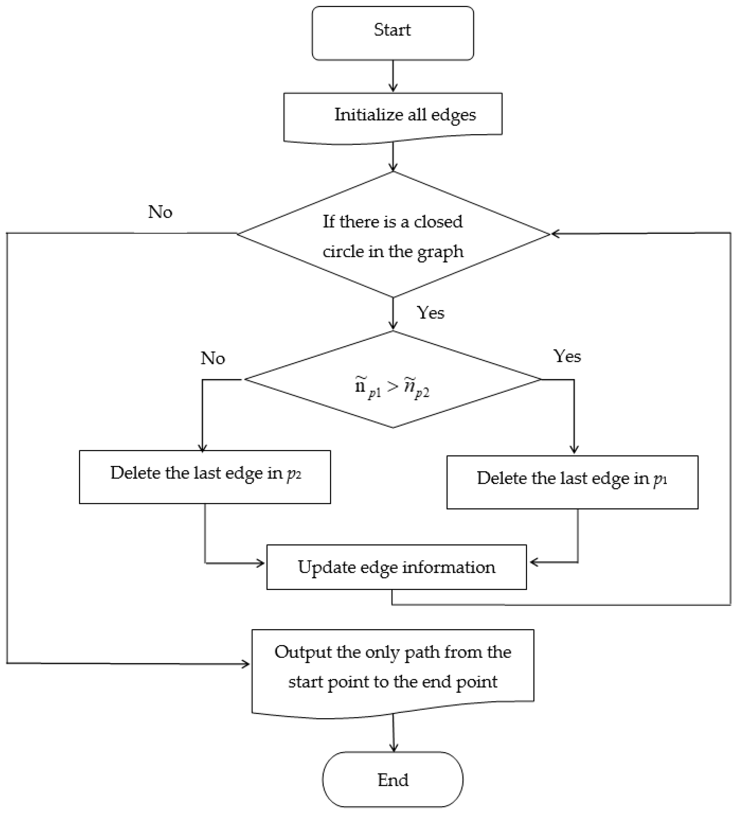
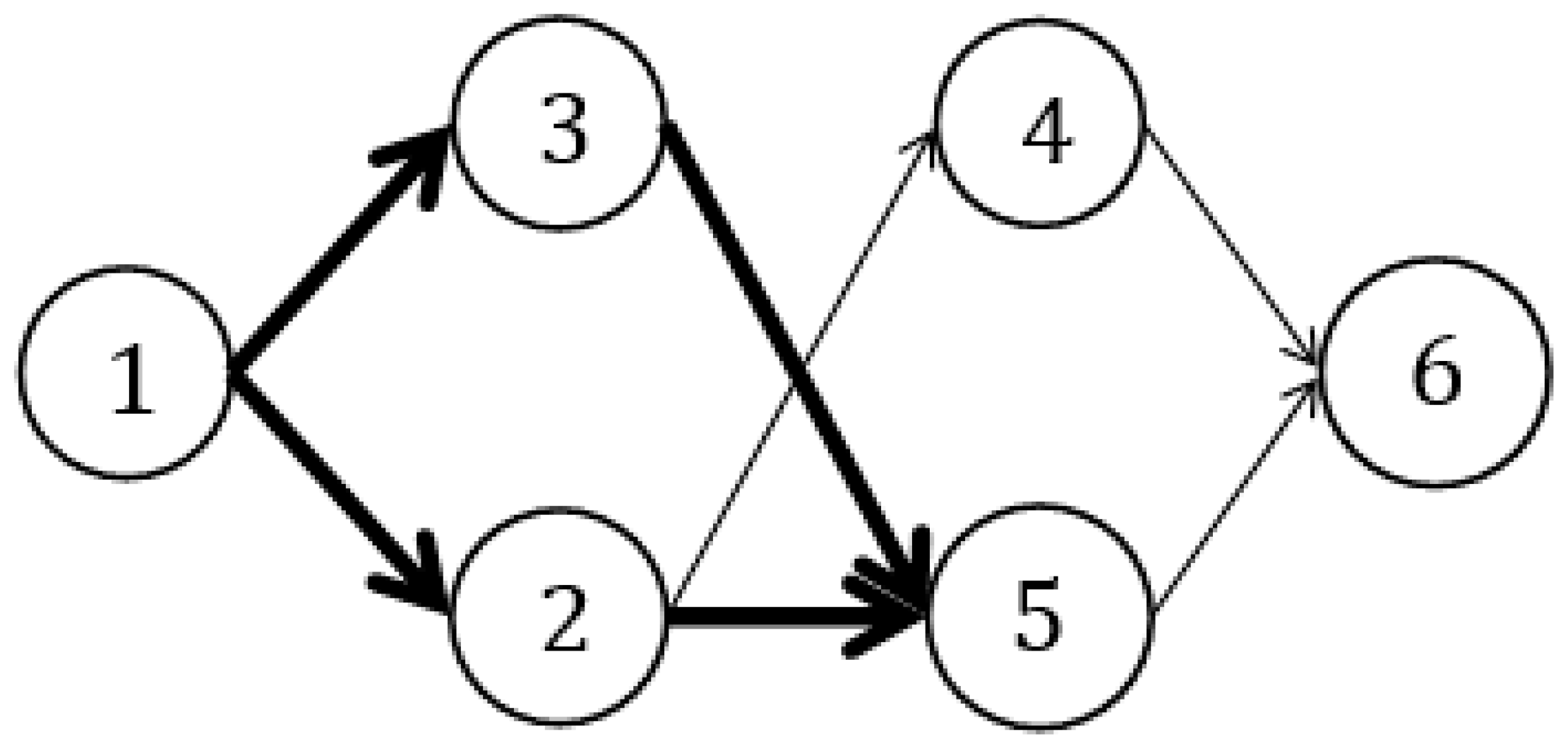
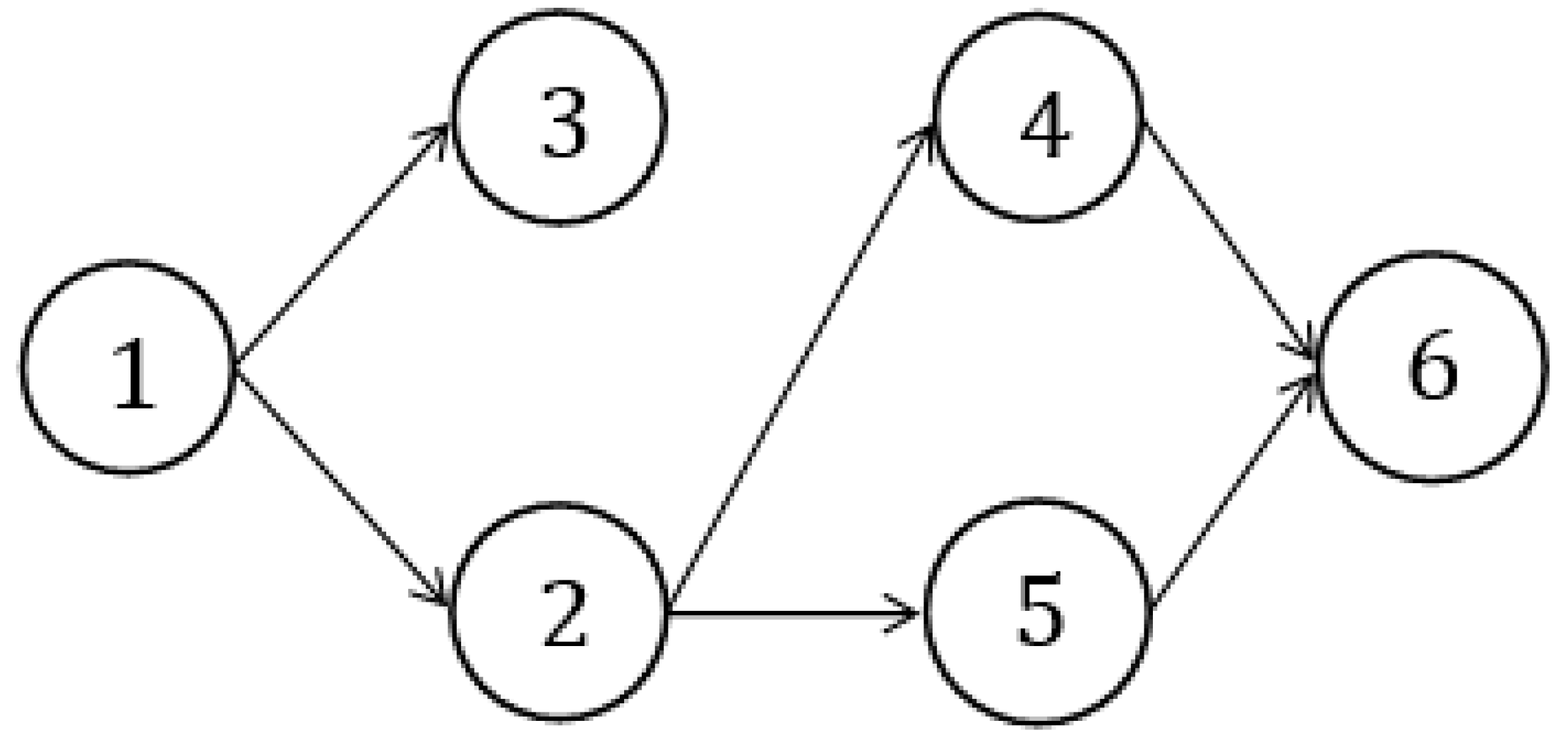
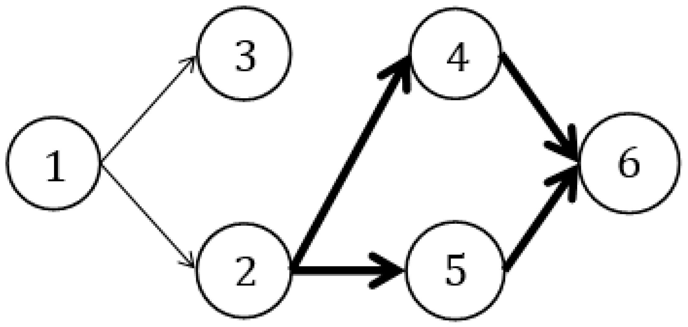
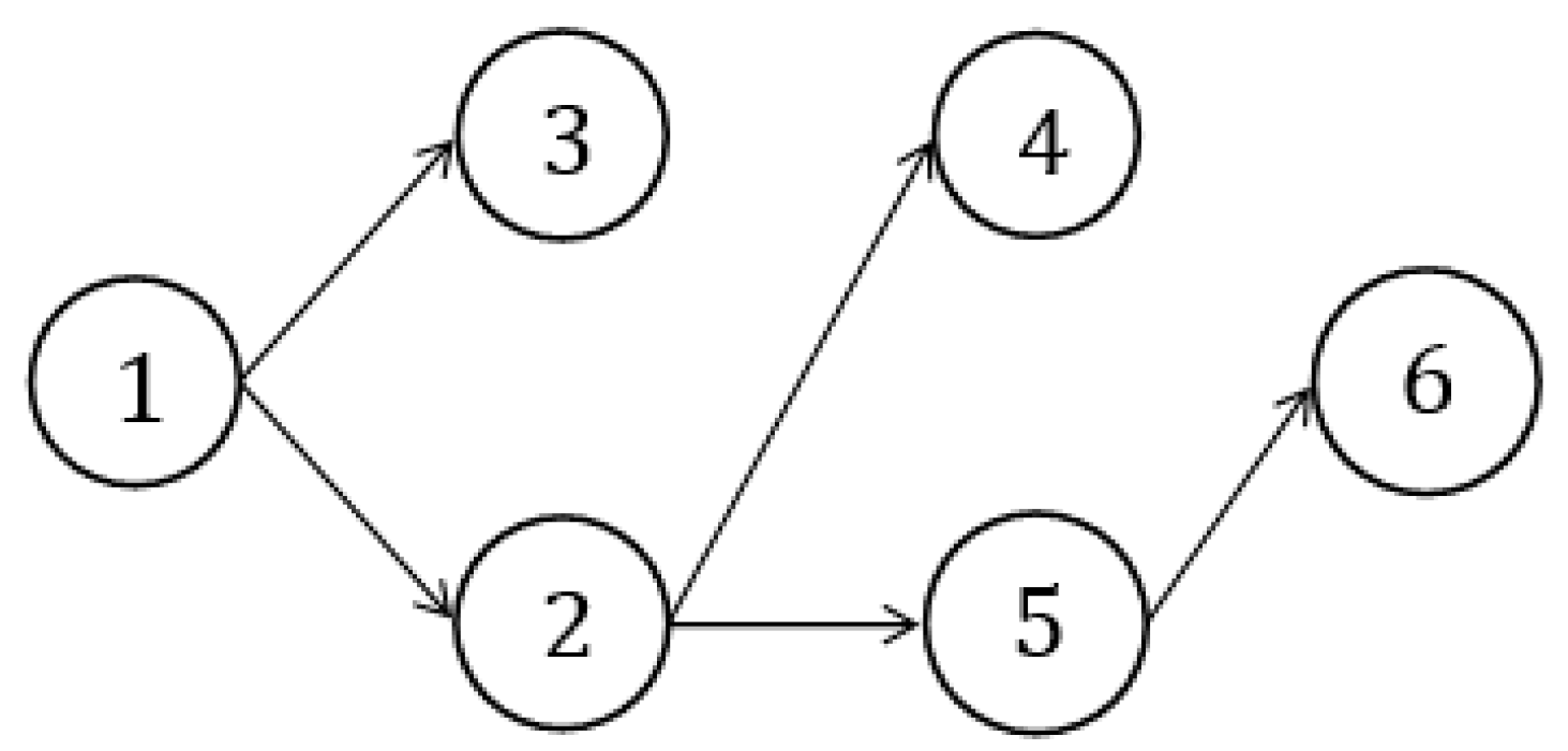
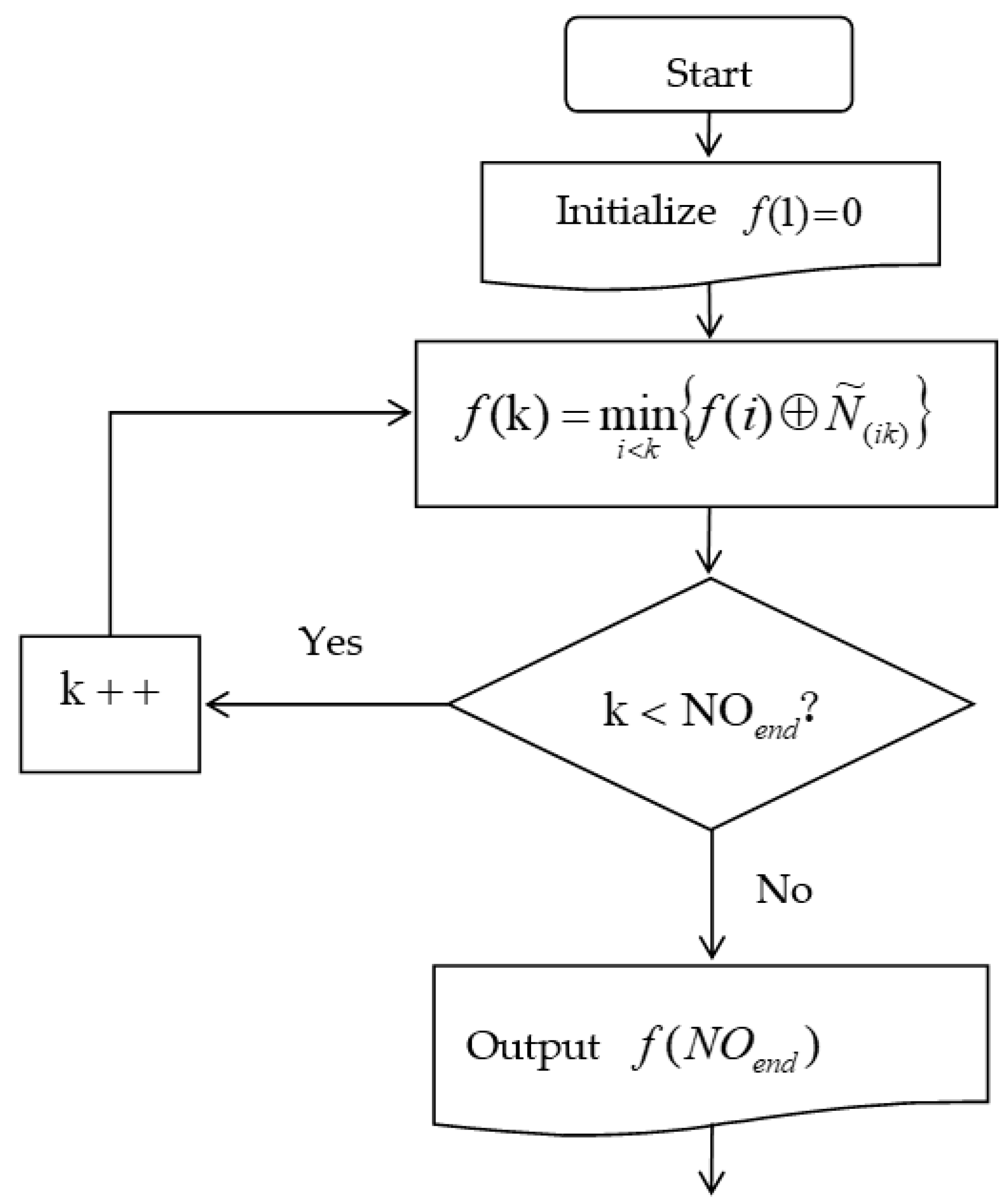
4. Method for Solving SPP of Trapezoidal Fuzzy Neutrosophic Graph Based on Circle-Breaking Algorithm

The circle-breaking algorithm can be used to solve the minimum cost spanning tree problem with weighted, connected, and undirected graphs. Furthermore, it can extend the SPP for directed graphs and search for a closed circle in the graphs, which is shared by the same starting and ending nodes. The end of the road is surrounded. A larger path can be found using Equations (9) and (10) as well as Definition 7. Subsequently, the last edge of the larger path is deleted and the above steps are repeated until there are no circles in the figure. The specific steps are as follows:

Step 1:

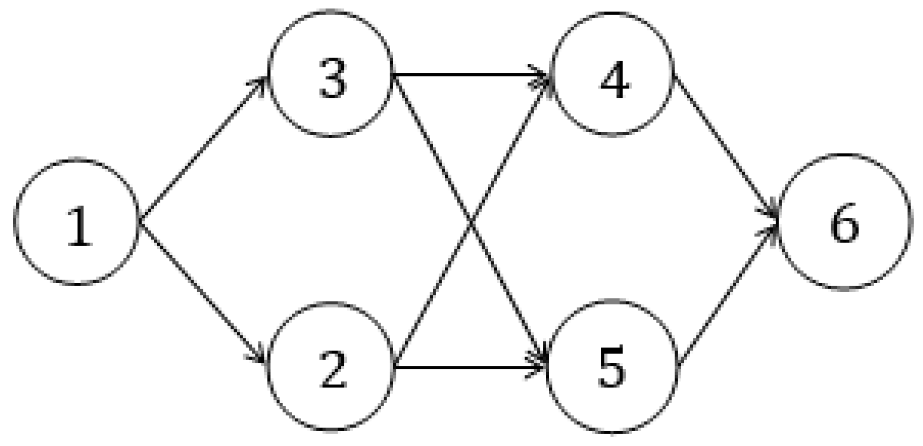
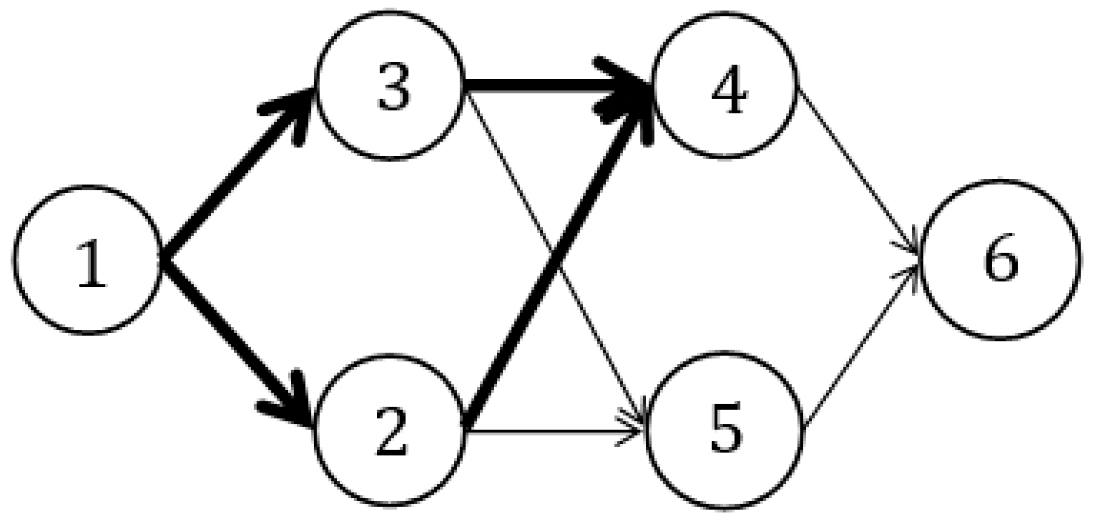
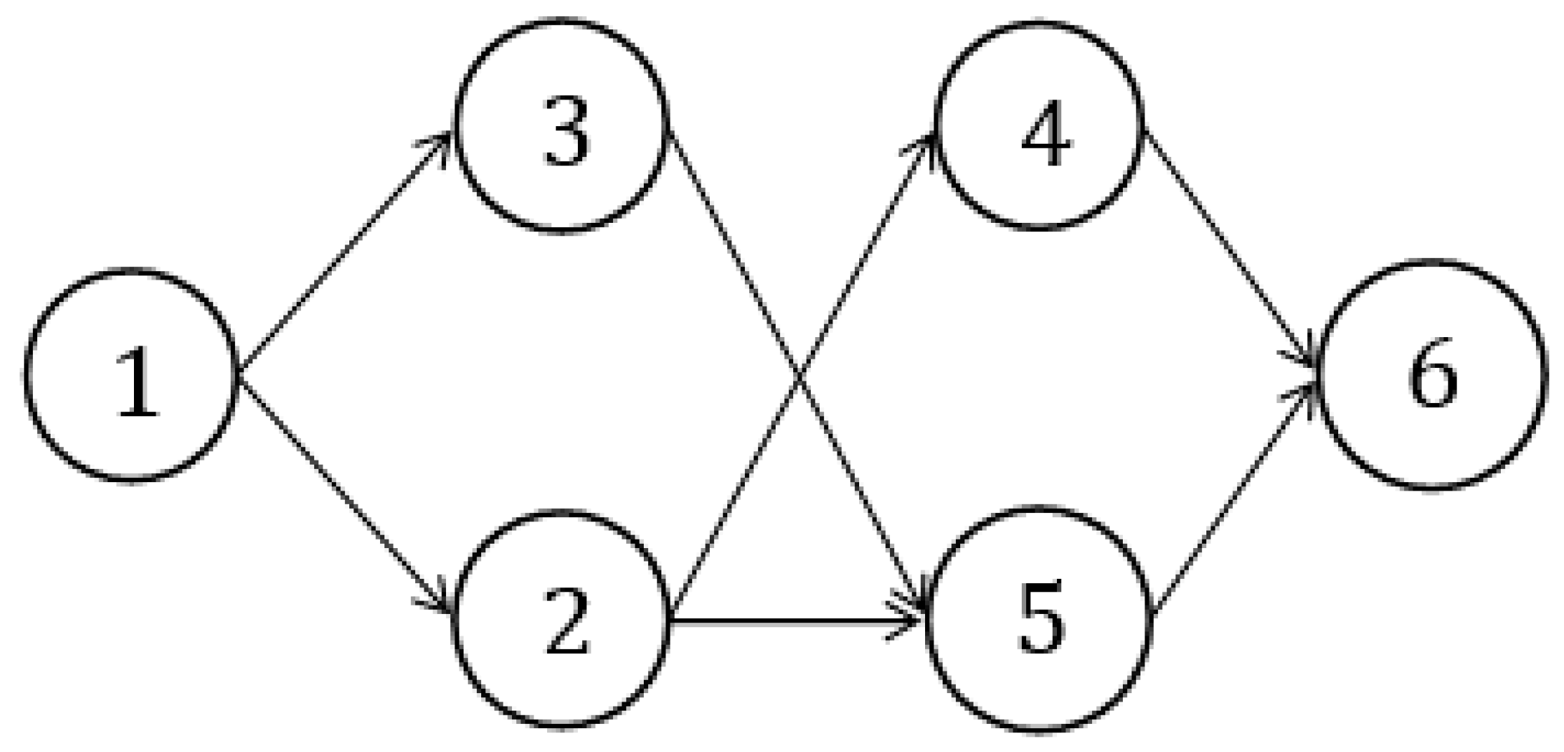
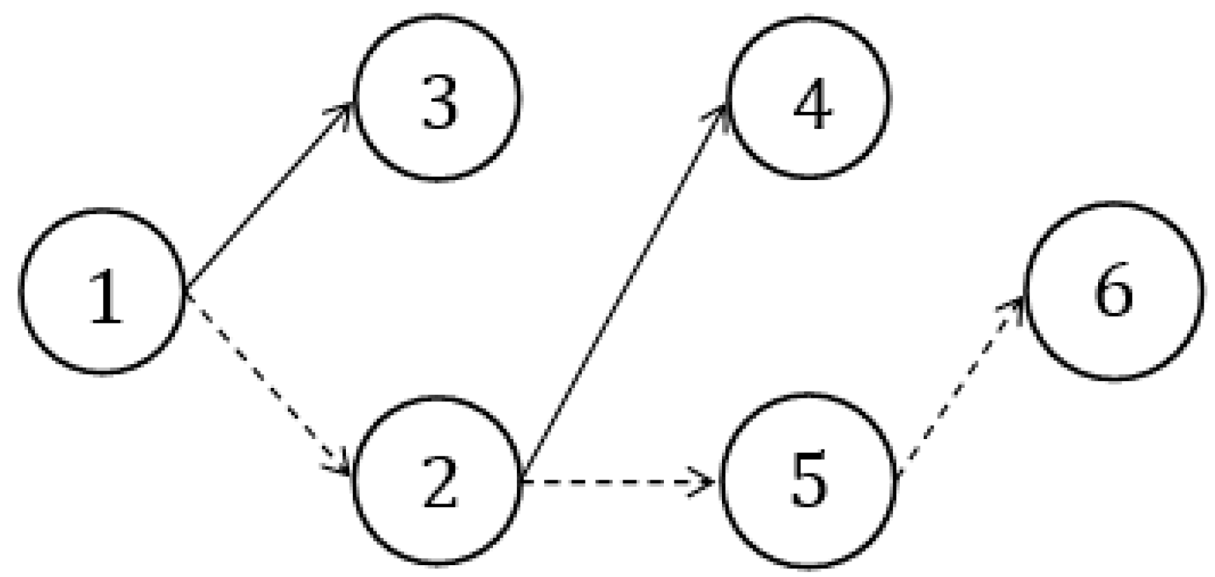
Arbitrarily define a closed circle in the trapezoidal fuzzy neutrosophic graph, and find the two paths p₁ and p₂ surrounding the closed circle, whereby p₁ and p₂ have a common starting node recorded as N₀ and a common ending node recorded as N₁.

Step 2:

According to Equation (5), all edges of each path are summed. The trapezoidal fuzzy numbers ${\tilde{n}}_{p1}$ and ${\tilde{n}}_{p2}$ are then obtained, which represent the two paths.

Step 3:

Obtain the score function value $S({\tilde{n}}_{p1})$ and exact function value $H({\tilde{n}}_{p1})$ of ${\tilde{n}}_{p1}$, as well as the score function value $S({\tilde{n}}_{p2})$ and exact function value $H({\tilde{n}}_{p2})$ of ${\tilde{n}}_{p2}$.

Step 4:

Compare the sizes of ${\tilde{n}}_{p1}$ and ${\tilde{n}}_{p2}$ according to the ranking function, and find and delete the edge in the larger path whose vertex is N1.

Step 5:

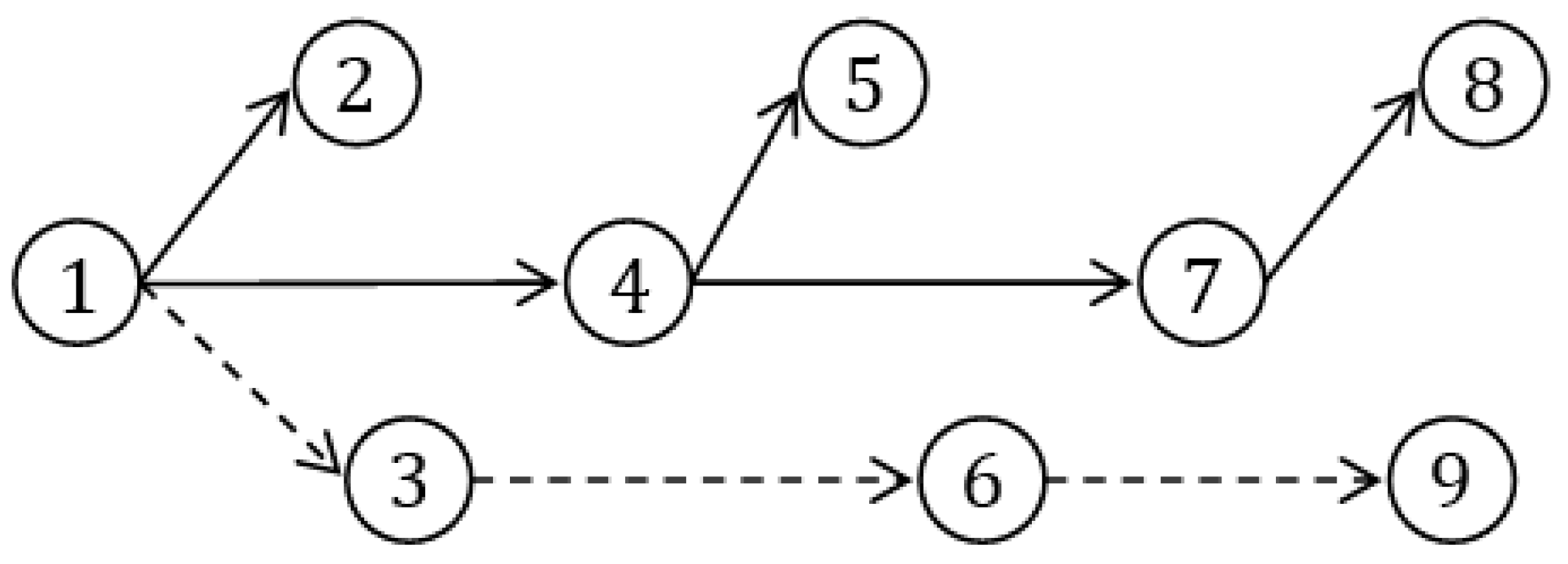
Determine whether a closed circle still exists on the map. If so, go to Step 1; if not, the algorithm terminates. At this time, only one path exists from the starting node to the ending node in the neutrosophic graph, which is the shortest path.

Figure 1 illustrates the flowchart of the circle-breaking algorithm according to the aforementioned steps:

In actual programming, determining whether a neutrosophic graph contains closed circles can be considered equivalent to judging whether there are vertices with in-degrees greater than one. If the in-degree of node i is greater than one, the predecessor is searched for based on the two edges pointing to node i. For node sets $R_1$ and $R_2$, there must be a vertex $k\in R_1\cap R_2$ that satisfies two different paths $p_1$ and $p_2$ from k to i. According to the flowchart in Figure 1, the pseudocode for calculating the designed Algorithm 1 circle-breaking algorithm is as follows:

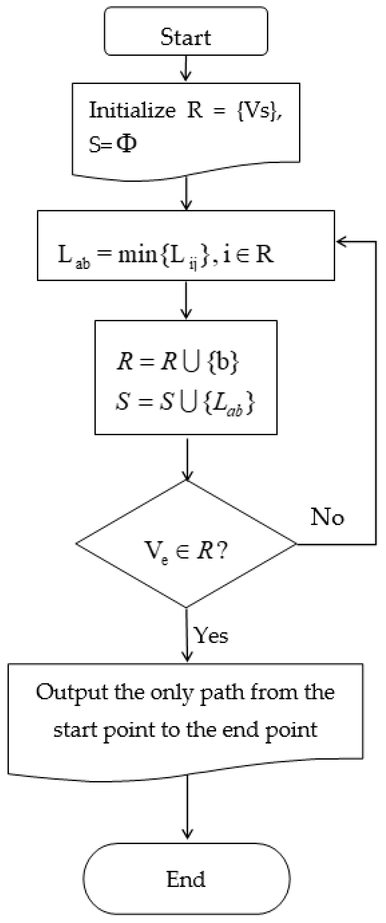
Algorithm 1 Circle-breaking Algorithm.

for i = N to 1   while(in-degree[i] > 1)    if(${\tilde{n}}_{p1}>{\tilde{n}}_{p2}$)     Delete the last edge in p1    else     Delete the last edge in p2   end while  end for

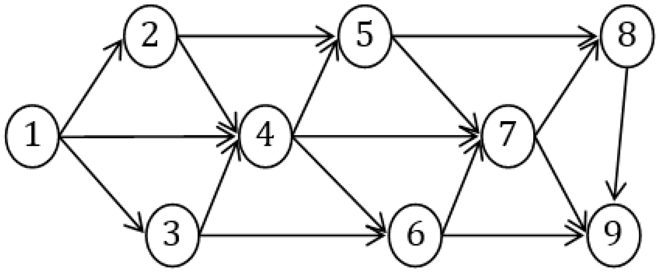
5. Case Study and Comparative Analysis

In this section, we describe the use of the circle-breaking algorithm to calculate two cases and compare this algorithm with other existing algorithms.

5.1. Case Analysis

Example 1. 

Since 20 July 2020, there has been a series of rainstorms in Wuhan City, China, with the maximum rainfall exceeding 100 mm. Owing to the rainstorms, waterlogging has become a major problem in many parts of Wuhan City, considerably hindering the traffic. According to Wuhan police, some sections of Huangpu Street, Fazhan Avenue, and Jiefang Avenue in Hankou, Wuhan are substantially waterlogged, resulting in traffic being blocked. The water under the light rail bridge of Huangpu Street is half a meter deep, preventing cars from passing and making it difficult to conduct rescue work. In view of the road conditions, it is necessary to identify the best paths to rescue points and provide decision support for the emergency rescue teams of the relevant departments. Figure 2 depicts the topological structure of the road network during this period, and

Table 1. Details of edge information in terms of trapezoidal fuzzy neutrosophic numbers (TrFNN).

Edges	Trapezoidal Fuzzy Neutrosophic Distances
(1, 2)	<(0.1, 0.2, 0.3, 0.5), (0.2, 0.3, 0.5, 0.6), (0.4, 0.5, 0.6, 0.8)>
(1, 3)	<(0.2, 0.4, 0.5, 0.7), (0.3, 0.5, 0.6, 0.9), (0.1, 0.2, 0.3, 0.4)>
(2, 4)	<(0.3, 0.4, 0.6, 0.7), (0.1, 0.2, 0.3, 0.5), (0.3, 0.5, 0.7, 0.9)>
(2, 5)	<(0.1, 0.3, 0.4, 0.5), (0.3, 0.4, 0.5, 0.7), (0.2, 0.3, 0.6, 0.7)>
(3, 4)	<(0.2, 0.3, 0.5, 0.6), (0.2, 0.5, 0.6, 0.7), (0.4, 0.5, 0.6, 0.8)>
(3, 5)	<(0.3, 0.6, 0.7, 0.8), (0.1, 0.2, 0.3, 0.4), (0.1, 0.4, 0.5, 0.6)>
(4, 6)	<(0.4, 0.6, 0.8, 0.9), (0.2, 0.4, 0.5, 0.6), (0.1, 0.3, 0.4, 0.5)>
(5, 6)	<(0.2, 0.3, 0.4, 0.5), (0.3, 0.4, 0.5, 0.6), (0.1, 0.3, 0.5, 0.6)>

presents the side lengths involved. The rescue team of Wuhan city must move from start point ① to end point ⑥ to rescue the trapped residents. Therefore, the objective of this example is to determine the shortest path from ① to ⑥.

The shortest path from ① to ⑥ is solved based on the circle-breaking algorithm in Figure 2. A circle is randomly selected in the figure, the larger of the two paths surrounding the circle is determined, and the last edge of the circle is deleted. This process is repeated until no other circle can be found. Finally, the only path remaining from ① to ⑥ is the shortest path.

Step 1: Circle ①②④③① in Figure 2 and paths $p_1=\{(1,3),(3,4)\}$ and $p_2=\{(1,2),(2,4)\}$ that make up the closed circle, as indicated by the thick lines in Figure 3, are found.

Step 2: According to Equation (5), all neutrosophic edges of each path are summed, and the TrFNN of the two paths are obtained by determining ${\tilde{n}}_{p_1}$ and ${\tilde{n}}_{p_2}$.

$$\begin{gathered} \begin{array}{l}{\tilde{n}}_{p1}={\tilde{n}}_{(1,3)}\oplus {\tilde{n}}_{(3,4)}\\ =\langle \begin{array}{l}\left(0.2+0.2-0.2*0.2,0.4+0.3-0.4*0.3,0.5+0.5-0.5*0.5,0.7+0.6-0.7*0.6\right),\\ \left(0.3*0.2,0.5*0.5,0.6*0.6,0.9*0.7\right),\\ \left(0.1*0.4,0.2*0.5,0.3*0.6,0.4*0.8\right)\end{array}\rangle \\ =<\left(0.36,0.58,0.75,0.88\right),\left(0.06,0.25,0.36,0.63\right),\left(0.04,0.1,0.18,0.32\right)>\end{array} \\ \begin{array}{l}{\tilde{n}}_{p2}={\tilde{n}}_{(1,2)}\oplus {\tilde{n}}_{(2,4)}\\ =\langle \begin{array}{l}\left(0.1+0.3-0.1*0.3,0.2+0.4-0.2*0.4,0.3+0.6-0.3*0.6,0.5+0.7-0.5*0.7\right),\\ \left(0.2*0.1,0.3*0.2,0.5*0.3,0.6*0.5\right),\\ \left(0.4*0.3,0.5*0.5,0.6*0.7,0.8*0.9\right)\end{array}\rangle \\ =<\left(0.37,0.52,0.72,0.85\right),\left(0.02,0.06,0.15,0.3\right),\left(0.12,0.25,0.42,0.72\right)>\end{array} \end{gathered}$$

Step 3: $S({\tilde{n}}_{p1})$, $H({\tilde{n}}_{p1})$, $S({\tilde{n}}_{p2})$, and $H({\tilde{n}}_{p2})$ are obtained.

$$\begin{gathered} \begin{array}{l}S({\tilde{n}}_{p1})\\ =\frac{1}{3}\left(2+\frac{0.36+0.58+0.75+0.88}{4}-\frac{0.06+0.25+0.36+0.63}{4}-\frac{0.04+0.1+0.18+0.32}{4}\right)\\ =0.719\end{array} \\ \begin{array}{l}S({\tilde{n}}_{p2})\\ =\frac{1}{3}\left(2+\frac{0.37+0.52+0.72+0.85}{4}-\frac{0.02+0.06+0.15+0.3}{4}-\frac{0.12+0.25+0.42+0.72}{4}\right)\\ =0.702\end{array} \\ H({\tilde{n}}_{p1})=\frac{0.36+0.58+0.75+0.88}{4}-\frac{0.04+0.1+0.18+0.32}{4}=0.483 \\ H({\tilde{n}}_{p2})=\frac{0.37+0.52+0.72+0.85}{4}-\frac{0.12+0.25+0.42+0.72}{4}=0.238 \end{gathered}$$

Step 4: Because $S({\tilde{n}}_{p1})>S({\tilde{n}}_{p2})$, ${\tilde{n}}_{p1}>{\tilde{n}}_{p2}$ can be obtained according to Definition 7. Thus, by deleting the last edge, (3, 4), in p₁, the neutrosophic graph in Figure 4 can be obtained.

Step 5: Closed circle ①②⑤③① in Figure 4 is selected, and paths $p_3=\{(1,3),(3,5)\}$ and $p_4=\{(1,2),(2,5)\}$ that make up the closed circle, as indicated by the thick lines in Figure 5, are obtained. Once this task is completed, we return to Step 2.

Step 2: According to Equation (5), all neutrosophic edges of each path are summed, and the TrFNN of the two paths are obtained by determining ${\tilde{n}}_{p3}$ and ${\tilde{n}}_{p4}$.

$$\begin{array}{l}{\tilde{n}}_{p3}={\tilde{n}}_{(1,3)}\oplus {\tilde{n}}_{(3,5)}\\ =\langle \begin{array}{l}\left(0.2+0.3-0.2*0.3,0.4+0.6-0.4*0.6,0.5+0.7-0.5*0.7,0.7+0.8-0.7*0.8\right),\\ \left(0.3*0.1,0.5*0.2,0.6*0.3,0.9*0.4\right),\\ \left(0.1*0.1,0.2*0.4,0.3*0.5,0.4*0.6\right)\end{array}\rangle \\ =<\left(0.44,0.76,0.85,0.94\right),\left(0.03,0.10,0.18,0.36\right),\left(0.01,0.08,0.15,0.24\right)>\end{array}$$

$$\begin{array}{l}{\tilde{n}}_{p4}={\tilde{n}}_{(1,2)}\oplus {\tilde{n}}_{(2,5)}\\ =\langle \begin{array}{l}\left(0.1+0.1-0.1*0.1,0.2+0.3-0.2*0.3,0.3+0.4-0.3*0.4,0.5+0.5-0.5*0.5\right),\\ \left(0.2*0.3,0.3*0.4,0.5*0.5,0.6*0.7\right),\\ \left(0.4*0.2,0.5*0.3,0.6*0.4,0.8*0.7\right)\end{array}\rangle \\ =<\left(0.19,0.44,0.58,0.75\right),\left(0.06,0.12,0.25,0.42\right),\left(0.08,0.15,0.24,0.56\right)>\end{array}$$

Step 3: Score function value $S({\tilde{n}}_{p3})$ and exact function value $H({\tilde{n}}_{p3})$ of ${\tilde{n}}_{p3}$, as well as score function value $S({\tilde{n}}_{p4})$ and exact function value $H({\tilde{n}}_{p4})$ of ${\tilde{n}}_{p4}$, are calculated.

$$\begin{array}{l}S({\tilde{n}}_{p3})\\ =\frac{1}{3}\left(2+\frac{0.44+0.76+0.85+0.94}{4}-\frac{0.03+0.10+0.18+0.36}{4}-\frac{0.01+0.08+0.15+0.24}{4}\right)\\ =0.820\end{array}$$

$$\begin{array}{l}S({\tilde{n}}_{p4})\\ =\frac{1}{3}\left(2+\frac{0.19+0.44+0.58+0.75}{4}-\frac{0.06+0.12+0.25+0.42}{4}-\frac{0.08+0.15+0.24+0.56}{4}\right)\\ =0.673\end{array}$$

$$H({\tilde{n}}_{p3})=\frac{0.44+0.76+0.85+0.94}{4}-\frac{0.01+0.08+0.15+0.24}{4}=0.628$$

$$H({\tilde{n}}_{p4})=\frac{0.19+0.44+0.58+0.75}{4}-\frac{0.08+0.15+0.24+0.56}{4}=0.233$$

Step 4: Because $S({\tilde{n}}_{p3})>S({\tilde{n}}_{p4})$, ${\tilde{n}}_{p3}>{\tilde{n}}_{p4}$ can be obtained according to Definition 7. Thus, by deleting the last edge, (3, 5), in p₃, the neutrosophic graph depicted in Figure 6 can be obtained.

Step 5: Another closed circle ②④⑥⑤② in Figure 6 is identified, such that paths $p_5=\{(2,4),(4,6)\}$ and $p_6=\{(2,5),(5,6)\}$ make up a closed circle, as indicated by the thick lines in Figure 7. Once this task is completed, we return to Step 2.

Step 2: According to Equation (5), all neutrosophic edges of each path are summed, and the TrFNN of the two paths are obtained by computing ${\tilde{n}}_{p5}$ and ${\tilde{n}}_{p6}$.

$$\begin{gathered} \begin{array}{l}{\tilde{n}}_{p5}={\tilde{n}}_{(2,4)}\oplus {\tilde{n}}_{(4,6)}\\ =\langle \begin{array}{l}\left(0.3+0.4-0.3*0.4,0.4+0.6-0.4*0.6,0.6+0.8-0.6*0.8,0.7+0.9-0.7*0.9\right),\\ \left(0.1*0.2,0.2*0.4,0.3*0.5,0.5*0.6\right),\\ \left(0.3*0.1,0.5*0.3,0.7*0.4,0.9*0.5\right)\end{array}\rangle \\ =<\left(0.58,0.76,0.92,0.97\right),\left(0.02,0.08,0.15,0.30\right),\left(0.03,0.15,0.28,0.45\right)>\end{array} \\ \begin{array}{l}{\tilde{n}}_{p6}={\tilde{n}}_{(2,5)}\oplus {\tilde{n}}_{(5,6)}\\ =\langle \begin{array}{l}\left(0.1+0.2-0.1*0.2,0.3+0.3-0.3*0.3,0.4+0.4-0.4*0.4,0.5+0.5-0.5*0.5\right),\\ \left(0.3*0.3,0.4*0.4,0.5*0.5,0.7*0.6\right),\\ \left(0.2*0.1,0.3*0.3,0.6*0.5,0.7*0.6\right)\end{array}\rangle \\ =<\left(0.28,0.51,0.64,0.75\right),\left(0.09,0.16,0.25,0.42\right),\left(0.02,0.09,0.30,0.42\right)>\end{array} \end{gathered}$$

Step 3: Score function value $S({\tilde{n}}_{p5})$ and exact function value $H({\tilde{n}}_5)$ of ${\tilde{n}}_{p5}$, as well as score function value $S({\tilde{n}}_{p6})$ and exact function value $H({\tilde{n}}_{p6})$ of ${\tilde{n}}_{p6}$ are obtained.

$$\begin{gathered} \begin{array}{l}S({\tilde{n}}_{p5})\\ =\frac{1}{3}\left(2+\frac{0.58+0.76+0.92+0.97}{4}-\frac{0.02+0.08+0.15+0.30}{4}-\frac{0.03+0.15+0.28+0.45}{4}\right)\\ =0.814\end{array} \\ \begin{array}{l}S({\tilde{n}}_{p6})\\ =\frac{1}{3}\left(2+\frac{0.28+0.51+0.64+0.75}{4}-\frac{0.09+0.16+0.25+0.42}{4}-\frac{0.02+0.09+0.30+0.42}{4}\right)\\ =0.703\end{array} \\ H({\tilde{n}}_{p5})=\frac{0.58+0.76+0.92+0.97}{4}-\frac{0.03+0.15+0.28+0.45}{4}=0.580 \\ H({\tilde{n}}_{p6})=\frac{0.28+0.51+0.64+0.75}{4}-\frac{0.02+0.09+0.30+0.42}{4}=0.338 \end{gathered}$$

Step 4: Because $S({\tilde{n}}_{p5})>S({\tilde{n}}_{p6})$, according to Definition 7, we can obtain ${\tilde{n}}_{p5}>{\tilde{n}}_{p6}$. The last edge, (4, 6), in p₅ is deleted, and the neutrosophic graph is obtained, as depicted in Figure 8.

Step 5: In the neutrosophic graph illustrated in Figure 8, it is no longer possible to find a closed circle and the circle-breaking algorithm ends. As indicated by the dotted line in Figure 9, only one path exists from starting node ① to ending node ⑥, which is the shortest path sought.

Example 2. 

The objective of this example is to determine the shortest path from starting node ① to ending node ⑨ in Figure 10. The edge weights are represented as TrFNN, and

Table 2. Details of edge information in terms of TrFNN.

Edges	Trapezoidal Fuzzy Neutrosophic Distance
(1, 2)	<(0.1, 0.3, 0.4, 0.5), (0.3, 0.5, 0.6, 0.7), (0.1, 0.3, 0.4, 0.6)>
(1, 3)	<(0.2, 0.4, 0.5, 0.7), (0.3, 0.5, 0.6, 0.9), (0.1, 0.2, 0.3, 0.4)>
(1, 4)	<(0.2, 0.3, 0.4, 0.6), (0.2, 0.4, 0.5, 0.6), (0.4, 0.5, 0.7, 0.8)>
(2, 4)	<(0.1, 0.3, 0.4, 0.5), (0.3, 0.4, 0.5, 0.7), (0.2, 0.3, 0.6, 0.7)>
(2, 5)	<(0.4, 0.5, 0.7, 0.8), (0.2, 0.3, 0.5, 0.6), (0.1, 0.2, 0.3, 0.5)>
(3, 4)	<(0.3, 0.6, 0.7, 0.8), (0.1, 0.2, 0.3, 0.4), (0.1, 0.4, 0.5, 0.6)>
(3, 6)	<(0.1, 0.2, 0.3, 0.4), (0.2, 0.4, 0.5, 0.6), (0.4, 0.5, 0.6, 0.7)>
(4, 5)	<(0.2, 0.3, 0.4, 0.5), (0.3, 0.4, 0.5, 0.6), (0.1, 0.3, 0.5, 0.6)>
(4, 6)	<(0.4, 0.6, 0.7, 0.9), (0.1, 0.2, 0.4, 0.5), (0.1, 0.3, 0.4, 0.6)>
(4, 7)	<(0.1, 0.3, 0.5, 0.6), (0.2, 0.3, 0.5, 0.7), (0.4, 0.5, 0.7, 0.8)>
(5, 7)	<(0.2, 0.3, 0.5, 0.6), (0.2, 0.5, 0.6, 0.7), (0.4, 0.5, 0.6, 0.8)>
(5, 8)	<(0.3, 0.5, 0.6, 0.7), (0.2, 0.3, 0.5, 0.6), (0.1, 0.2, 0.4, 0.5)>
(6, 7)	<(0.3, 0.4, 0.6, 0.7), (0.1, 0.2, 0.3, 0.5), (0.3, 0.5, 0.7, 0.9)>
(6, 9)	<(0.2, 0.3, 0.5, 0.6), (0.2, 0.3, 0.4, 0.5), (0.5, 0.6, 0.7, 0.9)>
(7, 8)	<(0.1, 0.2, 0.3, 0.5), (0.2, 0.3, 0.5, 0.6), (0.4, 0.5, 0.6, 0.8)>
(7, 9)	<(0.4, 0.6, 0.8, 0.9), (0.2, 0.4, 0.5, 0.6), (0.1, 0.3, 0.4, 0.5)>
(8, 9)	<(0.2, 0.3, 0.5, 0.6), (0.1, 0.2, 0.4, 0.5), (0.5, 0.6, 0.7, 0.8)>

lists the edge weight data. The circle-breaking algorithm is used to solve the SPP.

The removal of the last edge of the larger path in all closed circles using the circle-breaking algorithm enables the generation of the neutrosophic graph, as illustrated in Figure 11.

The path indicated by the dotted line is the shortest path from ① to ⑨.

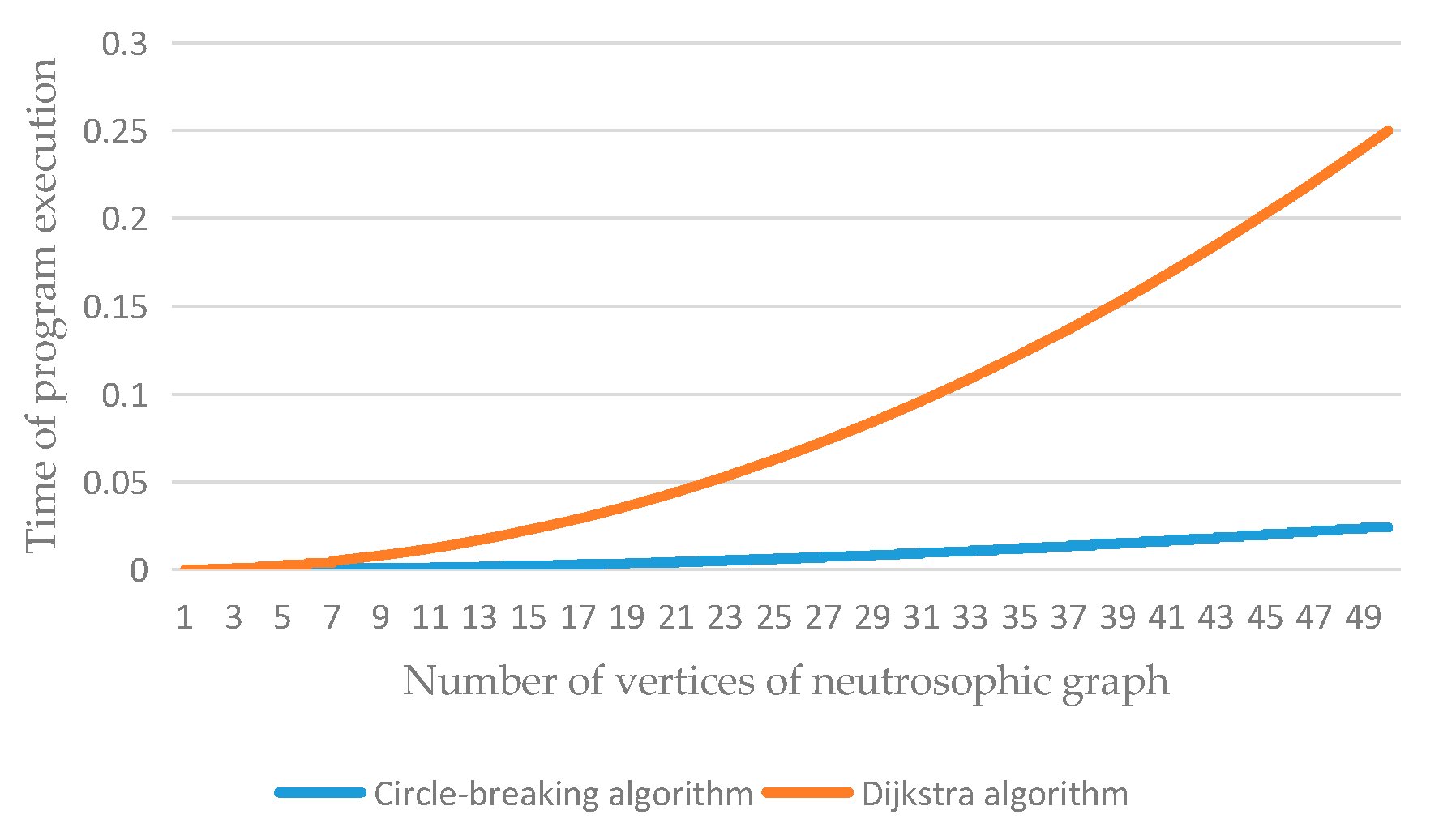
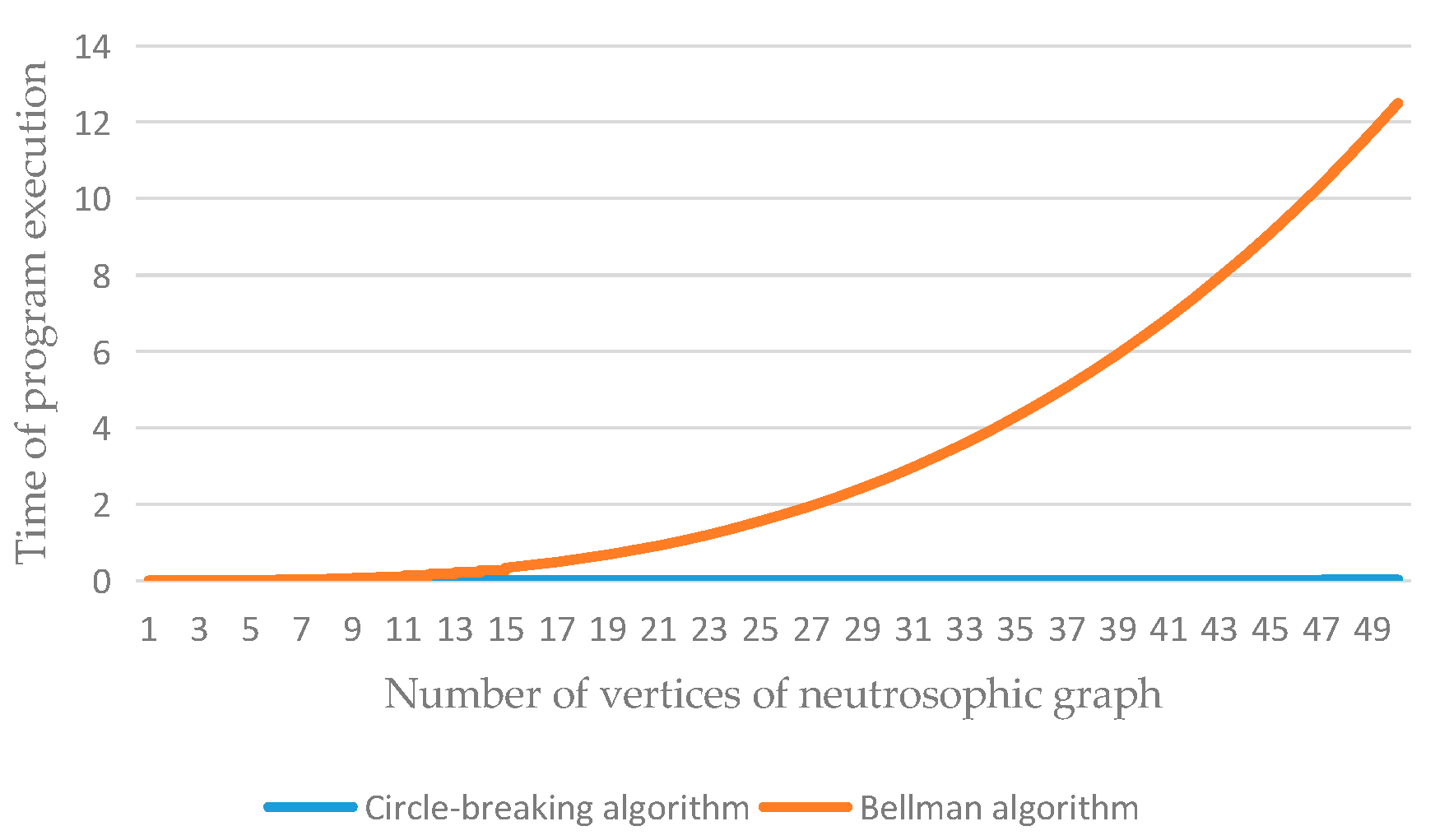
5.2. Comparative Analysis of Different Algorithms

1. To illustrate the validity and rationality of the algorithm, the circle-breaking algorithm proposed in this study is compared with the Dijkstra algorithm, and the adjacency matrix is established according to Table 1.

$$\left[\begin{array}{l}0.0,{\tilde{n}}_{(1,2)},{\tilde{n}}_{(1,3)},M,M,M\\ M,0.0,M,{\tilde{n}}_{(2,4)},{\tilde{n}}_{(2,5)},M\\ M,M,0.0,{\tilde{n}}_{(3,4)},{\tilde{n}}_{(3,5)},M\\ M,M,M,0.0,M,{\tilde{n}}_{(4,6)}\\ M,M,M,M,0.0,{\tilde{n}}_{(5,6)}\\ M,M,M,M,M,0.0\end{array}\right]$$

In this case, ${\tilde{n}}_{(i,j)}$ represents the edge weight from node i to node j. The specific values are listed in Table 1. M represents an infinite number, thereby indicating that no direct directed edge connection exists between nodes i and j.

Figure 12 illustrates the flowchart of the Dijkstra algorithm, where V_s represents the start point and V_e represents the end point.

Table 3. Shortest paths and their weights from starting node ① to all nodes (Example 1).

Nodes	Distance of Shortest Path	Shortest Path
②	$\langle \left(0.1,0.2,0.3,0.5\right),\left(0.2,0.3,0.5,0.6\right),\left(0.4,0.5,0.6,0.8\right)\rangle$	$➀\to ➁$
③	$\langle \left(0.2,0.4,0.5,0.7\right),\left(0.3,0.5,0.6,0.9\right),\left(0.1,0.2,0.3,0.4\right)\rangle$	$➀\to ➂$
④	$\langle \left(0.37,0.52,0.72,0.85\right),\left(0.02,0.06,0.15,0.30\right),\left(0.12,0.25,0.42,0.72\right)\rangle$	$➀\to ➁\to ➃$
⑤	$\langle \left(0.19,0.44,0.58,0.75\right),\left(0.06,0.12,0.25,0.42\right),\left(0.08,0.15,0.36,0.56\right)\rangle$	$➀\to ➁\to ➄$
⑥	$\langle \begin{array}{l}\left(0.352,0.608,0.748,0.875\right),\left(0.018,0.048,0.125,0.294\right),\\ \left(0.008,0.045,0.180,0.336\right)\end{array}\rangle$	$➀\to ➁\to ➄\to ➅$

displays the shortest path and the shortest path weights from starting node ① to all nodes using the existing Dijkstra algorithm: the shortest path from node ① to node ⑥ is $➀\to ➁\to ➄\to ➅$, and the weights are as follows:

$$\langle (0.352,0.608,0.748,0.875),(0.018,0.048,0.125,0.294),(0.008,0.045,0.180,0.336)\rangle$$

For the same calculation process, the shortest path and shortest path weights of starting node ① to all nodes in the second example are listed in

Table 4. Shortest paths and their weights from starting node ① to all nodes (Example 2).

Nodes	Distance of Shortest Path	Shortest Path
②	$<(0.1,0.3,0.4,0.5),(0.3,0.5,0.6,0.7),(0.1,0.3,0.4,0.6)>$	$➀\to ➁$
③	$<(0.2,0.4,0.5,0.7),(0.3,0.5,0.6,0.9),(0.1,0.2,0.3,0.4)>$	$➀\to ➂$
④	$<(0.2,0.3,0.4,0.6),(0.2,0.4,0.5,0.6),(0.4,0.5,0.7,0.8)>$	$➀\to ➃$
⑤	$\begin{array}{l}<(0.36,0.51,0.64,0.8),(0.06,0.16,0.25,0.36),\\ (0.04,0.15,0.35,0.48)>\end{array}$	$➀\to ➃\to ➄$
⑥	$\begin{array}{l}<\left(0.28,0.52,0.65,0.82\right),\left(0.06,0.2,0.3,0.54\right),\\ \left(0.04,0.1,0.18,0.28\right)>\end{array}$	$➀\to ➂\to ➅$
⑦	$\begin{array}{l}<\left(0.28,0.51,0.7,0.84\right),\left(0.04,0.12,0.25,0.42\right),\\ \left(0.16,0.25,0.49,0.64\right)>\end{array}$	$➀\to ➃\to ➆$
⑧	$\begin{array}{l}<\left(0.352,0.608,0.79,0.92\right),\left(0.008,0.036,0.125,0.252\right),\\ \left(0.064,0.125,0.294,0.512\right)>\end{array}$	$➀\to ➃\to ➆\to ➇$
⑨	$\begin{array}{l}<\left(0.424,0.664,0.825,0.928\right),\left(0.012,0.06,0.12,0.27\right),\\ \left(0.02,0.06,0.126,0.252\right)>\end{array}$	$➀\to ➂\to ➅\to ➈$

. The shortest path from node ① to node ⑨ is $➀\to ➂\to ➅\to ➈$, and the shortest path weights are $\langle \begin{array}{l}\left(0.424,0.664,0.825,0.928\right),\\ \left(0.012,0.06,0.12,0.27\right),\\ \left(0.02,0.06,0.126,0.252\right)\end{array}\rangle$.

2. Use of the enumeration algorithm in various examples

According to the adjacency matrix, all of the paths from node ① to node ⑥ are traversed. The distances of the neutrosophic edges of all paths are calculated according to Equation (5), and their score functions and exact functions are listed in

Table 5. List of all paths from node ① to node ⑥ (example 1).

Optional Path	Score Function	Exact Function
$p1:➀\to ➁\to ➃\to ➅$	0.872	0.686
$p2:➀\to ➁\to ➄\to ➅$	0.798	0.504
$p3:➀\to ➂\to ➃\to ➅$	0.871	0.780
$p4:➀\to ➂\to ➄\to ➅$	0.889	0.755

.

According to Definition 7, the edge distance of p₂ is the smallest, and the shortest path is $➀\to ➁\to ➄\to ➅$.

When using the enumeration algorithm to calculate the second example, there are 22 possible paths, and their scores and exact functions are calculated. The shortest path is $➀\to ➂\to ➅\to ➈$, and the shortest path distance is $\langle \begin{array}{l}\left(0.424,0.664,0.825,0.928\right),\left(0.012,0.06,0.12,0.27\right),\\ \left(0.02,0.06,0.126,0.252\right)\end{array}\rangle$.

3. Use of the Bellman algorithm in various examples

Here, $N{O}_{\mathrm{end}}$ is the number of the end point, ${\tilde{N}}_{(\mathrm{ij})}$ is the distance between point i and point j, and $f(i)$ is the shortest distance from point 1 to point i. Figure 13 shows the calculation flowchart of the Bellman algorithm in [31].

The calculation process for Case 1 is as follows:

$f(1)=0$,

$$\begin{gathered} \begin{array}{l}f(2)=\underset{i<2}{\min }\left\{f(i)\oplus {\tilde{N}}_{(i2)}\right\}=\min \left\{f(1)\oplus {\tilde{N}}_{(12)}\right\}\\ =\min \left\{0\oplus \langle (0.1,0.2,0.3,0.5),(0.2,0.3,0.5,0.7),(0.4,0.5,0.6,0.8)\rangle \right\}\\ =\langle (0.1,0.2,0.3,0.5),(0.2,0.3,0.5,0.7),(0.4,0.5,0.6,0.8)\rangle \end{array} \\ \begin{array}{l}f(3)=\underset{i<3}{\min }\left\{f(i)\oplus {\tilde{N}}_{(i3)}\right\}=\min \left\{f(1)\oplus {\tilde{N}}_{(13)}\right\}\\ =\min \left\{0\oplus \langle (0.2,0.4,0.5,0.7),(0.3,0.5,0.6,0.9),(0.1,0.2,0.3,0.4)\rangle \right\}\\ =\langle (0.2,0.4,0.5,0.7),(0.3,0.5,0.6,0.9),(0.1,0.2,0.3,0.4)\rangle \end{array} \\ \begin{array}{l}f(4)=\underset{i<4}{\min }\left\{f(i)\oplus {\tilde{N}}_{(i4)}\right\}\\ =\min \left\{f(2)\oplus {\tilde{N}}_{(24)},f(3)\oplus {\tilde{N}}_{(34)}\right\}\\ =\min \left\{\begin{array}{l}\langle (0.1,0.2,0.3,0.5),(0.2,0.3,0.5,0.7),(0.4,0.5,0.6,0.8)\rangle \oplus \\ \langle (0.3,0.4,0.6,0.7),(0.1,0.2,0.3,0.5),(0.3,0.5,0.7,0.9)\rangle ,\\ \langle (0.2,0.4,0.5,0.7),(0.3,0.5,0.6,0.9),(0.1,0.2,0.3,0.4)\rangle \oplus \\ \langle (0.2,0.3,0.5,0.6),(0.2,0.5,0.6,0.7),(0.4,0.5,0.6,0.8)\rangle \end{array}\right\}\\ =\min \left\{\begin{array}{l}\langle (0.37,0.58,0.62,0.85),(0.02,0.06,0.15,0.35),(0.12,0.25,0.42,0.72)\rangle ,\\ \langle (0.36,0.58,0.75,0.88),(0.06,0.25,0.36,0.63),(0.04,0.10,0.18,0.32)\rangle \end{array}\right\}\\ =\langle (0.37,0.58,0.62,0.85),(0.02,0.06,0.15,0.35),(0.12,0.25,0.42,0.72)\rangle \end{array} \\ \begin{array}{l}f(5)=\underset{i<5}{\min }\left\{f(i)\oplus {\tilde{N}}_{(i5)}\right\}\\ =\min \left\{f(2)\oplus {\tilde{N}}_{(25)},f(3)\oplus {\tilde{N}}_{(35)}\right\}\\ =\min \left\{\begin{array}{l}\langle (0.1,0.2,0.3,0.5),(0.2,0.3,0.5,0.7),(0.4,0.5,0.6,0.8)\rangle \oplus \\ \langle (0.1,0.3,0.4,0.5),(0.3,0.4,0.5,0.7),(0.2,0.3,0.6,0.7)\rangle ,\\ \langle (0.2,0.4,0.5,0.7),(0.3,0.5,0.6,0.9),(0.1,0.2,0.3,0.4)\rangle \oplus \\ \langle (0.3,0.6,0.7,0.8),(0.1,0.2,0.3,0.4),(0.1,0.4,0.5,0.6)\rangle \end{array}\right\}\\ =\min \left\{\begin{array}{l}\langle (0.19,0.44,0.58,0.75),(0.06,0.12,0.25,0.49),(0.08,0.15,0.36,0.56)\rangle ,\\ \langle (0.44,0.76,0.85,0.94),(0.03,0.10,0.18,0.36),(0.01,0.08,0.15,0.24)\rangle \end{array}\right\}\\ =\langle (0.19,0.44,0.58,0.75),(0.06,0.12,0.25,0.49),(0.08,0.15,0.36,0.56)\rangle \end{array} \\ \begin{array}{l}f(6)=\underset{i<6}{\min }\left\{f(i)\oplus {\tilde{N}}_{(i6)}\right\}\\ =\min \left\{f(4)\oplus {\tilde{N}}_{(46)},f(5)\oplus {\tilde{N}}_{(56)}\right\}\\ =\min \left\{\begin{array}{l}\langle (0.37,0.58,0.62,0.85),(0.02,0.06,0.15,0.35),(0.12,0.25,0.42,0.72)\rangle \oplus \\ \langle (0.4,0.6,0.8,0.9),(0.2,0.4,0.5,0.6),(0.1,0.3,0.4,0.5)\rangle ,\\ \langle (0.19,0.44,0.58,0.75),(0.06,0.12,0.25,0.49),(0.08,0.15,0.36,0.56)\rangle \oplus \\ \langle (0.2,0.3,0.4,0.5),(0.3,0.4,0.5,0.6),(0.1,0.3,0.5,0.6)\rangle \end{array}\right\}\\ =\min \left\{\begin{array}{l}\langle (0.622,0.832,0.924,0.985),(0.004,0.024,0.075,0.210),(0.012,0.075,0.168,0.360)\rangle ,\\ \langle (0.352,0.608,0.748,0.875),(0.018,0.048,0.125,0.294),(0.008,0.045,0.180,0.336)\rangle \end{array}\right\}\\ =\langle (0.352,0.608,0.748,0.875),(0.018,0.048,0.125,0.294),(0.008,0.045,0.180,0.336)\rangle \end{array} \end{gathered}$$

Thus,

$$\begin{array}{l}f(6)=f(5)\oplus {\tilde{N}}_{(56)}\\ =f(2)\oplus {\tilde{N}}_{(25)}\oplus {\tilde{N}}_{(56)}\\ =f(1)\oplus {\tilde{N}}_{(12)}\oplus {\tilde{N}}_{(25)}\oplus {\tilde{N}}_{(56)}\\ ={\tilde{N}}_{(12)}\oplus {\tilde{N}}_{(25)}\oplus {\tilde{N}}_{(56)}\end{array}$$

Therefore, path $p_{(1256)}$ is recognized as the neutrosophic shortest path, its neutrosophic distance is $\langle \begin{array}{l}(0.352,0.608,0.748,0.875),\\ (0.018,0.048,0.125,0.294),\\ (0.008,0.045,0.180,0.336)\end{array}\rangle$, and its score function and exact function are

$$\begin{gathered} S(p_{(1256)})=\frac{1}{3}\times \left(\begin{array}{l}2+\frac{0.352+0.608+0.748+0.875}{4}\\ -\frac{0.018+0.048+0.125+0.294}{4}\\ -\frac{0.008+0.045+0.180+0.336}{4}\end{array}\right)=0.794 \\ H(p_{(1256)})=\frac{0.352+0.608+0.748+0.875}{4}-\frac{0.008+0.045+0.180+0.336}{4}=0.504 \end{gathered}$$

respectively.

The same calculation process can be used to determine

$$\begin{array}{l}f(9)=f(6)\oplus {\tilde{N}}_{(69)}=f(3)\oplus {\tilde{N}}_{(36)}\oplus {\tilde{N}}_{(69)}\\ =f(1)\oplus {\tilde{N}}_{(13)}\oplus {\tilde{N}}_{(36)}\oplus {\tilde{N}}_{(69)}\\ ={\tilde{N}}_{(13)}\oplus {\tilde{N}}_{(36)}\oplus {\tilde{N}}_{(69)}\end{array}$$

Its shortest path is p₍₁₃₆₉₎.

Based on the comparison of the four algorithms, the proposed circle-breaking algorithm is equivalent to the Dijkstra and enumeration algorithms, achieving the same shortest path and shortest path distance. Additionally, the implementation of the algorithm is feasible and reasonable. Moreover, the circle-breaking algorithm is easy to understand, and its implementation is relatively simple.

Furthermore, from the perspective of the time complexity of the algorithm, the Bellman algorithm is a two-layer loop, and the inner loop includes one iteration; therefore, the time complexity of the Bellman algorithm is $O(n^3)$. In contrast, the circle-breaking and Dijkstra algorithms are both two-layer loops with a time complexity of $O(n^2)$; however, there is no inevitable sequence for evaluating the in-degree of all vertices in the circle-breaking algorithm. Nevertheless, multithreaded or distributed programming can be employed to reduce the time complexity of the algorithm. Therefore, we use the code of the circle-breaking algorithm; when run using 10 threads, the time complexity of the algorithm can be reduced to $O(n^2)/10$. The pseudocode of the Algorithm 2 circle-breaking algorithm is as follows:

Algorithm 2 Multi-threaded realization of circle-breaking algorithm

Class Circle-breaking extends Thread{  public Circle-breaking(int k){    for(int i = (k − 1)*N/10, i < k*N/10, i++)    {     while(in-degree[i] > 1)     {      if(${\tilde{n}}_{p1}>{\tilde{n}}_{p2}$)      {       Delete the last edge in p1      }      else      {       Delete the last edge in p2      }     }    }   }  }   public static void main(String[] args) {    Circle-breaking[] c = new Circle-breaking [10];    for(int i = 0; i < c.length; i++)    {     c[i] = new Circle-breaking(i + 1);     c[i].start();    }  }

Assuming that the computer requires 0.0001 s to perform a calculation, the execution times of the program when using the circle-breaking, Dijkstra, and Bellman algorithms are determined, as depicted in Figure 14 and Figure 15.

In these figures, the abscissa represents the number of vertices of the neutrosophic graph, and the ordinate represents the running time of the algorithm. As shown in Figure 14 and Figure 15, in the case of the same number of vertices in the neutrosophic graph, the running time of the circle-breaking algorithm is lesser than those of the Dijkstra and Bellman algorithms. Hence, the circle-breaking algorithm is feasible and reasonable.

6. Conclusions

In this study, we developed a circle-breaking algorithm for solving the SPP of a trapezoidal fuzzy neutrosophic graph and verified the feasibility of the algorithm using an example. Furthermore, we compared the algorithm with the Bellman and Dijkstra algorithms and obtained a consistent shortest path, thereby demonstrating the effectiveness of the algorithm. Finally, we compared the operating efficiencies of the three algorithms and proved that the circle-breaking algorithm could achieve better operating efficiency through multithreaded or distributed programming. In the future, we intend to appropriately sort the in-degrees of the nodes when initializing the data for further efficiency improvement.

References

1. Ahuja, R.K.; Mehlhorn, K.; Orlin, J.; Tarjan, R.E. Faster algorithms for the shortest path problem. J. ACM 1990, 37, 213–223. [Google Scholar] [CrossRef] [Green Version]
2. Dubois, D.; Prade, H.; Yager, R.R. Fuzzy Information Engineering: A Guided Tour of Applications; John Wiley and Sons: New York, NY, USA, 1997. [Google Scholar]
3. Biswas, S.S.; Alam, B.; Doja, M.N. Intuitionistic Fuzzy Real Time Multigraphs for Communication Networks: A Theoretical Model. In Proceedings of the 2013 AASRI Conference on Parallel and Distributed Computing and Systems, Singapore, 1–3 May 2013; pp. 114–119. [Google Scholar]
4. Gabrel, V.; Murat, C.; Wu, L. New models for the robust shortest path problem: Complexity, resolution and generalization. Ann. Oper. Res. 2013, 207, 97–120. [Google Scholar] [CrossRef]
5. Grigoryan, H.; Harutyunyan, H.A. The shortest path problem in the Knödel graph. J. Discret. Algorithms 2015, 31, 40–47. [Google Scholar] [CrossRef]
6. Broumi, S.; Bakali, A.; Talea, M.; Smarandache, F. Isolated Single Valued Neutrosophic Graphs. Neutrosophic Sets Syst. 2016, 11, 74–78. [Google Scholar]
7. Rajashi, C.; Pinaki, M.; Syamal, K.S. Interval-Valued Possibility Quadripartitioned Single Valued Neutrosophic Soft Sets and Some Uncertainty Based Measures on Them. Neutrosophic Sets Syst. 2016, 14, 35–43. [Google Scholar]
8. Buckley, J.; Jowers, L.J. Fuzzy shortest path problem. Monte Carlo methods in fuzzy optimization. Stud. Fuzziness Soft Comput. 2007, 222, 191–193. [Google Scholar]
9. Deng, Y.; Chen, Y.; Zhang, Y.; Mahadevan, S. Fuzzy Dijkstra algorithm for shortest path problem under uncertain environment. Appl. Soft Comput. 2012, 12, 1231–1237. [Google Scholar] [CrossRef]
10. Ye, J. Multiple-attribute decision-making method under a single-valued neutrosophic hesitant fuzzy environment. J. Intell. Syst. 2014, 24, 23–36. [Google Scholar] [CrossRef]
11. Peng, J.J.; Wang, J.Q. Multi-valued Neutrosophic Sets and its Application in Multi-criteria Decision-making Problems. Neutrosophic Sets Syst. 2015, 10, 3–17. [Google Scholar] [CrossRef]
12. Ye, J. Trapezoidal neutrosophic set and its application to multiple attribute decision-making. Neural Comput. Appl. 2015, 26, 1157–1166. [Google Scholar] [CrossRef]
13. Nancy; Harish, G. An improved score function for ranking neutrosophic sets and its application to decision making process. Int. J. Uncertain. Quantfication 2016, 6, 377–385. [Google Scholar] [CrossRef]
14. Broumi, S.; Bakali, A.; Talea, M.; Smarandache, F.; Verma, R. Computing Minimum Spanning Tree in Interval Valued Bipolar Neutrosophic Environment. Int. J. Model. Optim. 2017, 7, 300–304. [Google Scholar] [CrossRef]
15. Peng, X.D.; Dai, J.G. Algorithms for interval neutrosophic multiple attribute decision-making based on MABAC, similarity measure, and EDAS. Int. J. Uncertain. Quantfication 2017, 7, 395–421. [Google Scholar] [CrossRef] [Green Version]
16. Smarandache, F. A Unifying Field in Logics: Neutrosophic Logic, Neutrosophic Set, Neutrosophic Probability and Statistics, 4th ed.; American Research Press: Rehoboth, DE, USA, 1998. [Google Scholar]
17. Wang, H.B.; Smarandache, F.; Zhang, Y.Q.; Sunderraman, R. Single valued neutrosophic sets. Tech. Sci. Appl. Math. 2012, 20, 10–14. [Google Scholar]
18. Deli, I.; Şubaş, Y. A ranking method of single valued neutrosophic numbers and its applications to multi-attribute decision making problems. Int. J. Mach. Learn. Cyb. 2017, 8, 1309–1322. [Google Scholar]
19. Broumi, S.; Bakali, A.; Bahnasse, A. Neutrosophic sets: On overview. New Trends Neutrosophic Theor. Appl. 2018, 2, 403–434. [Google Scholar]
20. Broumi, S.; Bakali, A.; Talea, M.; Smarandache, F.; Ali, M. Shortest Path Problem under Bipolar Neutrosphic Setting. Appl. Mech. Mater. 2017, 859, 59–66. [Google Scholar] [CrossRef]
21. Bolturk, E.; Kahraman, C. A novel interval-valued neutrosophic AHP with cosine similarity measure. Soft Comput. 2018, 22, 4941–4958. [Google Scholar] [CrossRef]
22. Biswas, P.; Pramanik, S.; Giri, B.C. Distance measure based MADM strategy with interval trapezoidal neutrosophic numbers. Neutrosophic Sets Syst. 2018, 19, 40–46. [Google Scholar]
23. Deli, I. Expansions and reductions on neutrosophic classical soft set. Süleyman Demirel U. J. Nat. Appl. Sci. 2018, 22, 478–486. [Google Scholar] [CrossRef]
24. Deli, I. Operators on single valued trapezoidal neutrosophic numbers and SVTN-group decision making. Neutrosophic Sets Syst. 2018, 22, 131–151. [Google Scholar]
25. Deli, I.; Şubaş, Y. Some weighted geometric operators with SVTrN-numbers and their application to multi-criteria decision making problems. J. Intell. Fuzzy Syst. 2017, 32, 291–301. [Google Scholar] [CrossRef] [Green Version]
26. Basset, M.A.; Atef, A.; Smarandache, F. A hybrid neutrosophic multiple criteria group decision making approach for project selection. Cogn. Syst. Res. 2019, 57, 216–227. [Google Scholar] [CrossRef]
27. Basset, M.A.; Mohamed, M.; Sangaiah, A.K. Neutrosophic AHPDelphi Group decision making model based on trapezoidal neutrosophic numbers. J. Amb. Intel. Hum. Comp. 2017, 9, 1427–1443. [Google Scholar] [CrossRef] [Green Version]
28. Kumar, R.; Edaltpanah, S.A.; Jha, S.; Broumi, S. Neutrosophic shortest path problem. Neutrosophic Sets Syst. 2018, 23, 5–15. [Google Scholar]
29. Broumi, S.; Bakali, A.; Talea, M.; Smarandache, F.; Kishore, P.K.; Şahin, R. Shortest path problem under interval valued neutrosophic setting. Int. J. Adv. Trends Comput. Sci. Eng. 2019, 8, 216–222. [Google Scholar]
30. Tan, R.P.; Zhang, W.D.; Broumi, S. Solving methods for the shortest path problem based on trapezoidal fuzzy neutrosophic numbers. Control Decis. 2019, 34, 851–860. [Google Scholar]
31. Broumi, S.; Dey, A.; Talea, M.; Bakali, A.; Smarandache, F.; Nagarajan, D.; Lathamaheswari, M.; Kumar, R. Shortest path problem using Bellman algorithm under neutrosophic environment. Complex Intell. Syst. 2019, 5, 409–416. [Google Scholar] [CrossRef] [Green Version]
32. Chakraborty, A. Application of Pentagonal Neutrosophic Number in Shortest Path Problem. Int. J. Neutrosophic Sci. 2020, 3, 21–28. [Google Scholar]
33. Schweizer, P. Uncertainty: Two probabilities for the three states of neutrosophy. Int. J. Neutrosophic Sci. 2020, 2, 18–26. [Google Scholar]
34. Edalatpanah, S.A. A Direct Model for Triangular Neutrosophic Linear Programming. Int. J. Neutrosophic Sci. 2020, 1, 19–28. [Google Scholar]
35. Yang, L.H.; Li, D.M.; Tan, R.P. Research on the Shortest Path Solution Method of Interval Valued Neutrosophic Graphs Based on the Ant Colony Algorithm. IEEE Access 2020, 8, 88717–88728. [Google Scholar] [CrossRef]
36. Guan, M.G. Algorithm of breaking circle for minimum tree. J. Math. Pract. Theory 1975, 4, 40–43. [Google Scholar]
37. Zeng, J.B.; Zhang, W.; Li, X.Y. Islanding Algorithm of Distribution System with Distributed Generations based on Circle-breaking Algorithm. Power Sys. Eng. 2019, 35, 15–19. [Google Scholar]
Figure 1. Flowchart of the circle-breaking algorithm.
Symmetry 12 01360 g001
Figure 2. Trapezoidal fuzzy neutrosophic graph.
Symmetry 12 01360 g002
Figure 3. Closed circle ①②④③①.
Symmetry 12 01360 g003
Figure 4. Removal of edge (3, 4).
Symmetry 12 01360 g004
Figure 5. Closed circle ①②⑤③①.
Symmetry 12 01360 g005
Figure 6. Removal of edge (3, 5).
Symmetry 12 01360 g006
Figure 7. Closed circle ②④⑥⑤②.
Symmetry 12 01360 g007
Figure 8. Removal of edge (4, 6).
Symmetry 12 01360 g008
Figure 9. Shortest path of example 1.
Symmetry 12 01360 g009
Figure 10. Trapezoidal fuzzy neutrosophic graph.
Symmetry 12 01360 g010
Figure 11. Shortest path of example 2.
Symmetry 12 01360 g011
Figure 12. Flowchart of the Dijkstra algorithm.
Symmetry 12 01360 g012
Figure 13. Flowchart of the Bellman algorithm.
Symmetry 12 01360 g013
Figure 14. Comparison of the execution times of the circle-breaking and Dijkstra algorithms.
Symmetry 12 01360 g014
Figure 15. Comparison of the execution times of the circle-breaking and Bellman algorithms.
Symmetry 12 01360 g015