Discrete-Inverse Optimal Control Applied to the Ball and Beam Dynamical System: A Passivity-Based Control Approach

Abstract

This express brief deals with the problem of the state variables regulation in the ball and beam system by applying the discrete-inverse optimal control approach. The ball and beam system model is defined by a set of four-order nonlinear differential equations that are discretized using the forward difference method. The main advantages of using the discrete-inverse optimal control to regulate state variables in dynamic systems are (i) the control input is an optimal signal as it guarantees the minimum of the Hamiltonian function, (ii) the control signal makes the dynamical system passive, and (iii) the control input ensures asymptotic stability in the sense of Lyapunov. Numerical simulations in the MATLAB environment allow demonstrating the effectiveness and robustness of the studied control design for state variables regulation with a wide gamma of dynamic behaviors as a function of the assigned control gains.

1. Introduction

The ball and beam dynamical system is a classical and well-known nonlinear dynamical system that attracts much attention in the control area [1]. The main challenge in this plant is to regulate all the state variables at the origin, taking into account that it corresponds to a fourth-order dynamical system ($n=4$) with only one control input ($m=1$) [2]. Additionally, the system contains strong nonlinearities such as products between variables and trigonometric functions [3]. Analyzing the ball and beam system from the control analysis point of view is interesting as its model can be used to understand transportation systems, communication, or power system dynamics [4]. In the literature, the problem of control in ball and beam systems has been addressed with linear and nonlinear techniques with some of these are presented as follows; proportional-integral control [5], feedback of state variables [6], linear matrix inequalities [7] exact feedback linearization [8], control Lyapunov functions [9,10], adaptive control design [2], passivity-based control [11], fuzzy logic [12,13], and artificial neural networks [14], among others.

The main contributions of our approach, different from previous works, can be summarized as follows [15].

✔

The application of the discrete-inverse optimal control to regulate all the state variables of the ball and beam system guaranteeing passivity, stability, and optimality properties.

✔

The numerical validation via simulations by working the discrete equivalent nonlinear model of the system without any special assumption on the open- or closed-loop dynamics.

✔

The robustness and effectiveness of the discrete-inverse optimal control design when parametric variations affect the discrete dynamical model.

It is important to mention that after an exhaustive revision of the literature about the ball and beam dynamical system modeling and control, we identify that the discrete-inverse optimal control has not been studied in this system. This indicates that it is a clear opportunity for research that this article tries to fill.

The remainder of this document is organized as follows. Section 2 presents the general dynamical formulation for the ball and beam dynamical system on the continuous and discrete domains. Section 3 presents the general theory about discrete-inverse optimal control applied on nonlinear systems by highlighting its passivity, stability, and optimality properties. Section 4 shows all the numerical simulations and their corresponding analysis and discussion. Section 5 presents the main conclusions derived from this research study.

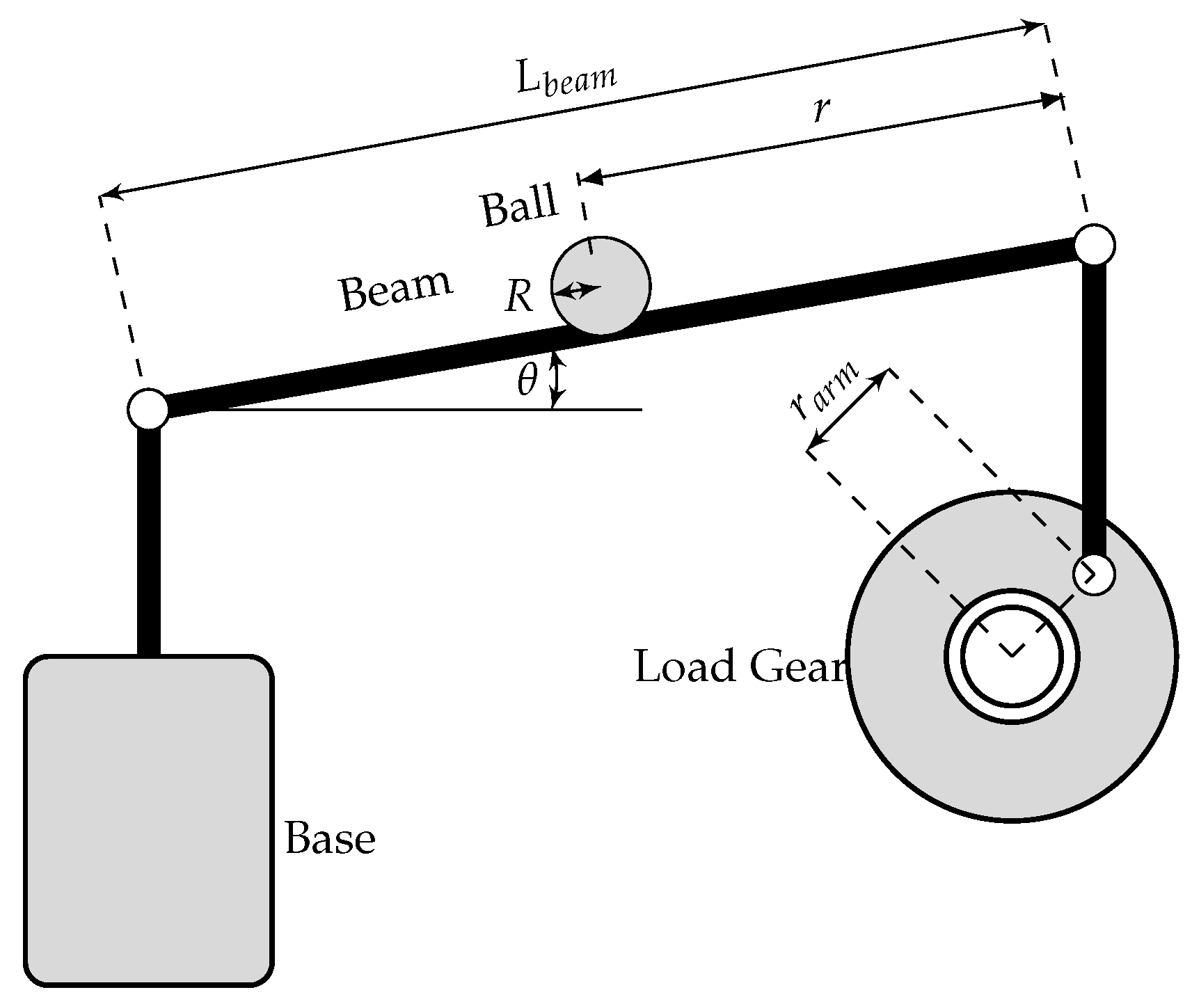
2. Dynamical Model and Discretization

The ball and beam system generates a fourth-order nonlinear set of ordinary nonlinear differential equations [2]. The main objective is to regulate all the state variables around the origin of coordinates guaranteeing stability in closed-loop. Figure 1 illustrates the physical form of the ball and beam system.

In this figure the variables and parameters have the following interpretation; $\theta$ and r are the beam angle and the ball position, respectively. Moreover, $k_1$ is the steady-state gain; $\tau$ is the time-constant, $L_{\mathrm{beam}}$ is the length of the beam; and m and $J_b$ are the mass and moment of inertia of the ball, respectively. In addition, R is the radius of the ball, g is the acceleration due to gravity, $r_{\mathrm{arm}}$ is the distance between screw and motor gear, and $V_m$ is the input of the system [2]. The dynamical formulation of the ball and beam system depicted in Figure 1 is presented below.

$$\ddot{r}=\frac{m{r}_{\mathrm{arm}}g{R}^2}{L_{\mathrm{beam}}\left(m{R}^2+J_b\right)}sin\left(\theta \right)-\frac{m}{\frac{J_b}{R^2}+m}r{\dot{\theta }}^2,$$

(1a)

$$\ddot{\theta }=-\frac{1}{\tau }\dot{\theta }+\frac{k_1}{\tau }{v}_m,$$

(1b)

To reach the state space representation of the dynamical model (1), let us define $k_{bb}=\frac{m{r}_{\mathrm{arm}}g{R}^2}{L_{\mathrm{beam}}\left(m{R}^2+J_b\right)}$, $h=\frac{m}{\frac{J_b}{R^2}+m}$, and ${\left[x_1,x_2,x_3,x_4\right]}^T={\left[r,\dot{r},\theta ,\dot{\theta }\right]}^T$, which allows finding the following fourth-order nonlinear dynamical model,

$${\dot{x}}_1=x_2,$$

(2a)

$${\dot{x}}_2=k_{bb}sin\left(x_3\right)-h{x}_1{x}_4^2,$$

(2b)

$${\dot{x}}_3=x_4,$$

(2c)

$${\dot{x}}_4=-\frac{1}{\tau }{x}_4+\frac{k_1}{\tau }u,$$

(2d)

where $u=v_m$ corresponds to the control input. Note that the equilibrium point of the dynamical system (2) is ${\left[x_1^{🟉},x_2^{🟉},x_3^{🟉},x_4^{🟉}\right]}^T={\left[r_0,0,0,0\right]}^T$, being $r_0$ an arbitrary point between the extremes of the beam; nevertheless, the unique physical solution possible is when $r_0=0$, due to the gravity force in the real system will make any other point unstable as can be seen in Figure 1.

To design the proposed controller it is needed to represent the continuous dynamical system (2) into a discrete equivalent. For doing so, the classical forward difference is applied [16], i.e.,

$$\begin{array}{c}\hfill \dot{x}=f\left(x\right)\leftrightarrow x_{k+1}={\Delta }_{k}f\left(x_k\right)+x_k,\end{array}$$

where subscript k is the current sample and ${\Delta }_k$ represents the discretization time. If we apply the forward difference in the set of Equations (2), the the following discrete system is reached. l

$$x_{1_{k+1}}={\Delta }_k{x}_{2_k}+x_{1_k},$$

(3a)

$$x_{2_{k+1}}={\Delta }_k\left(k_{bb}sin\left(x_{3_k}\right)-h{x}_{1_k}{x}_{4_k}^2\right)+x_{2_k},$$

(3b)

$$x_{3_{k+1}}={\Delta }_k{x}_{4_k}+x_{3_k},$$

(3c)

$$x_{4_{k+1}}={\Delta }_k\left(-\frac{1}{\tau }{x}_{4_k}+\frac{k_1}{\tau }{u}_k\right)+x_{4_k},$$

(3d)

3. Inverse Optimal Control Design

In this section three main aspects of the inverse optimal control design will be explored for general nonlinear discrete systems [15,17]. For doing so, let us define the general structure of the system under analysis as follows [18,19].

Definition 1.

A nonlinear dynamical system in the discrete domain with the form,

$$x_{k+1}=f\left(x_k\right)+g\left(x_k\right)u_k,$$

(4a)

$$y_k=h\left(x_k\right)+j\left(x_k\right)u_k,$$

(4b)

fulfills passivity properties, is globally asymptotically stable, and also there is a control law with the form $u_k=-y_k$, such that a functional cost function is minimized, i.e., $u_k$ is an optimal control law. Note that in (4), $y_k$ is the output of the system and $h\left(x_k\right)$ and $j\left(x_k\right)$ take the followings structures,

$$h\left(x_k\right)=g^T\left(x_k\right)\mathit{P}f\left(x_k\right),$$

(5a)

$$j\left(x_k\right)=\frac{1}{2}{g}^T\left(x_k\right)\mathit{P}g\left(x_k\right)$$

(5b)

being Q a symmetry positive definite matrix, i.e., $\mathit{P}={\mathit{P}}^T\succ 0$.

To demonstrate each one of the properties presented in Definition 1, let us consider a candidate Lyapunov function with a quadratic form as follows,

$$\begin{array}{c}\hfill \mathcal{V}\left(x_k\right)=\frac{1}{2}{x}_k^T\mathbf{P}{x}_k,\end{array}$$

(6)

which is positive definite for all $x_k\ne 0$ and zero only for $x_k=0$. In addition, let us define a general form for the control input $u_k$ as follows,

$$\begin{array}{c}\hfill u_k=\beta \left(x_k\right)+v_k,\end{array}$$

(7)

where $v_k$ is the new input and $\beta \left(x_k\right)$ can be defined as presented below,

$$\begin{array}{c}\hfill \beta \left(x_k\right)=-{\left(I+j\left(x_k\right)\right)}^{-1}h\left(x_k\right),\end{array}$$

(8)

being I an identity matrix with appropriate dimensions.

Definition 2.

The dynamical system (4) exhibits passivity properties if there is a matrix P such that the following inequality is held.

$$\begin{array}{cc}\hfill {\left(f\left(x_k\right)+g\left(x_k\right)\beta \left(x_k\right)\right)}^T\mathit{P}\left(f\left(x_k\right)+g\left(x_k\right)\beta \left(x_k\right)\right)\le x_k^T\mathit{P}{x}_k& ,\hfill \end{array}$$

(9)

3.1. Passivity

To demonstrate passivity properties in the the dynamical discrete system consider Lemma 1 as presented below [20,21,22].

Theorem 1.

The dynamical system in (4) is a feedback passive system for the output ${\tilde{y}}_k$. The control input is defined as (7), where ${\tilde{y}}_k$ takes the following form,

$$\begin{array}{c}\hfill {\tilde{y}}_k=\tilde{h}\left(x_k\right)+j\left(x_k\right)v_k.\end{array}$$

(10)

where

$$\tilde{h}\left(x_k\right)=g^T\left(x_k\right)\mathit{P}\tilde{f}\left(x_k\right),$$

(11a)

$$\tilde{f}\left(x_k\right)=f\left(x_k\right)+g\left(x_k\right)\beta \left(x_k\right)$$

(11b)

Proof. 

To proof the feedback passivity properties of the dynamical system (4), consider the variation of the Lyapunov function for the current and the future states as follows,

$$\begin{array}{c}\hfill \Delta \mathcal{V}=\mathcal{V}\left(x_{k+1}\right)-\mathcal{V}\left(x_k\right).\end{array}$$

(12)

Note that using (4) and (7) in (12), we have

$$\begin{array}{r}\Delta \mathcal{V}=\frac{1}{2}{\left(f\left(x_k\right)+g\left(x_k\right)\beta \left(x_k\right)\right)}^T\mathbf{P}\left(f\left(x_k\right)+g\left(x_k\right)\beta \left(x_k\right)\right)\\ -\frac{1}{2}{x}_k^T\mathbf{P}{x}_k+{\left(f\left(x_k\right)+g\left(x_k\right)\beta \left(x_k\right)\right)}^T\mathbf{P}g\left(x_k\right)v_k+\\ \frac{1}{2}{v}_k^T{g}^T\left(x_k\right)\mathbf{P}g\left(x_k\right)v_k.\end{array}$$

(13)

From (13), we can observe that

$${\left(f\left(x_k\right)+g\left(x_k\right)\beta \left(x_k\right)\right)}^T\mathbf{P}g\left(x_k\right)v_k={\tilde{h}}^T\left(x_k\right)v_k,$$

(14a)

$$v_k^T{g}^T\left(x_k\right)\mathbf{P}g\left(x_k\right)v_k=2v_k^T{j}^T\left(x_k\right)v_k.$$

(14b)

Now, if we consider Definition 2 and expressions in (14) to be replaced in (13), then we have

$$\begin{array}{c}\hfill \Delta \mathcal{V}\le {\tilde{y}}_k^T{v}_k,\end{array}$$

(15)

which confirms that the discrete system is passive from the output ${\tilde{y}}_k$ to the new input $v_k$ and the proof about passivity is completed. □

3.2. Stability

To demonstrate passivity properties the stability properties in the sense of Lyapunov for closed-loop operation, let us consider the following Lemma.

Theorem 2.

The system (4) is asymptotically stable in the sense of Lyapunov with the control input (7) if $v_k$ is defined as

$$\begin{array}{c}\hfill v_k=-{\tilde{y}}_k=-{\left(I+j\left(x_k\right)\right)}^{-1}\tilde{h}\left(x_k\right).\end{array}$$

(16)

Proof. 

To proof stability in the sense of Lyapunov, we can transform the dynamical system (4) with the control input (7) as an equivalent system with the following structure

$$x_{k+1}=\tilde{f}\left(x_k\right)+g\left(x_k\right)w_k.$$

(17)

Now, if we consider the difference between the current and the next step of the Lyapunov function defined in (12), we have

$$\begin{array}{r}\Delta \mathcal{V}=\frac{1}{2}{\left(\tilde{f}\left(x_k\right)+g\left(x_k\right)w_k\right)}^T\mathbf{P}\left(\tilde{f}\left(x_k\right)+g\left(x_k\right)w_k\right)\\ -\frac{1}{2}{x}_k^T\mathbf{P}{x}_k={\tilde{f}}^T\left(x_k\right)\mathbf{P}g\left(x_k\right)v_k+\frac{1}{2}{v}_k^T{g}^T\left(x_k\right)\mathbf{P}g\left(x_k\right)v_k+\\ \frac{1}{2}\left({\tilde{f}}^T\left(x_k\right)\mathbf{P}\tilde{f}\left(x_k\right)-x_k^T\mathbf{P}{x}_k\right).\end{array}$$

(18)

From (18), we can note that

$$\begin{array}{c}\hfill {\tilde{f}}^T\left(x_k\right)\mathbf{P}g\left(x_k\right)v_k+\frac{1}{2}{v}_k^T{g}^T\left(x_k\right)\mathbf{P}g\left(x_k\right)v_k={\tilde{y}}_k^T{v}_k,\end{array}$$

(19)

in addition, from Lemma 2, we know that $v_k=-{\tilde{y}}_k$, which implies that in conjunction with (19), the expression (18) takes the following form

$$\begin{array}{c}\hfill \Delta \mathcal{V}=\frac{1}{2}\left({\tilde{f}}^T\left(x_k\right)\mathbf{P}\tilde{f}\left(x_k\right)-x_k^T\mathbf{P}{x}_k\right)-{\left|\left|v_k\right|\right|}^2<0,\end{array}$$

(20)

which allows to conclude that the system (4) is globally asymptotically stable in $x_k=0$ as the candidate Lyapunov function $\mathcal{V}\left(x_k\right)=\frac{1}{2}{x}_k^T\mathbf{P}{x}_k$ is radially unbounded. This completes the proof. □

3.3. Optimality

Theorem 3.

The inverse control law (7) is considered optimal since it stabilizes the dynamical system as presented in Section 3.2, and it minimizes the following functional cost

$$\begin{array}{c}\hfill \mathcal{F}=\sum _{k=0}^{\infty }\mathcal{L}\left(x_k,\beta \left(x_k\right)\right),\end{array}$$

(21)

where $L\left(x_k,\beta \left(x_k\right)\right)$ is the LaGrangian function of the system that can be written as

$$\begin{array}{c}\hfill \mathcal{L}\left(x_k,\beta \left(x_k\right)\right)=l\left(x_k\right)+{\beta }^T\left(x_k\right)\beta \left(x_k\right).\end{array}$$

(22)

being $l\left(x_k\right)$ defined as

$$\begin{array}{c}\hfill l\left(x_k\right)=\frac{x_k^T\mathit{P}{x}_k-{\tilde{f}}^T\left(x_k\right)\mathit{P}\tilde{f}\left(x_k\right)}{2},\end{array}$$

(23)

Note that the optimal solution for the functional cost is ${\mathcal{F}}^{🟉}=\mathcal{V}\left(x_0\right)$, being it $x_0$ the initial condition for the dynamical system (4).

Proof. 

To demonstrate the control law $\beta \left(x_k\right)$, that is, an optimal function, let us consider the Hamiltonian of the system as

$$\begin{array}{c}\hfill \mathcal{H}\left(x_k,u_k\right)=\mathcal{L}\left(x_k,\beta \left(x_k\right)\right)+\mathcal{V}\left(x_{k+1}\right)-\mathcal{V}\left(x_k\right),\end{array}$$

(24)

which has the global minimum as $\frac{\partial \mathcal{H}\left(x_k,u_k\right)}{\partial u_k}=0$.

To minimize this Hamiltonian function, we can rewrite (23) considering (22) as follows,

$$\begin{array}{c}\hfill \underset{\beta \left(x_k\right)}{min}\left\{l\left(x_k\right)+{\beta }^T\left(x_k\right)\beta \left(x_k\right)+\mathcal{V}\left(x_{k+1}\right)-\mathcal{V}\left(x_k\right)\right\}=0.\end{array}$$

(25)

The solution of the minimization function (25) considering (23) and the variation of the candidate Lyapunov function (12) as presented in [18], it is taken the following form,

$$\begin{array}{r}-h^T\left(x_k\right)+2{\beta }^T\left(x_k\right)j\left(x_k\right)+\\ \left(f^T\left(x_k\right)-y_k^T{g}^T\left(x_k\right)\right)\mathbf{P}g\left(x_k\right)=0,\end{array}$$

(26)

in addition, if we consider (4b) and (5), then we can simplify (27) as presented below,

$$\begin{array}{c}\hfill {\beta }^T\left(x_k\right)j\left(x_k\right)+h^T\left(x_k\right)j\left(x_k\right)+{\beta }^T\left(x_k\right)j^T\left(x_k\right)j\left(x_k\right)=0.\end{array}$$

(27)

It is important to mention that the solution of (27) for $\beta \left(x_k\right)$ takes the following structure,

$$\begin{array}{c}\hfill \beta \left(x_k\right)=-{\left(I+j\left(x_k\right)\right)}^{-1}h\left(x_k\right),\end{array}$$

(28)

which confirms control function initially defined in (8) as an optimal control law as it minimizes the functional cost (21).

In order to determine the optimal value for the Lagrangian function (21), let us consider that the interval of analysis $\left[0,N\right]$, being N a natural number with the following result,

$$\begin{array}{c}\hfill \sum _{k=0}^{\infty }\mathcal{L}\left(x_k,\beta \left(x_k\right)\right)=-\mathcal{V}\left(x_N\right)+\mathcal{V}\left(x_0\right)+\sum _{k=0}^{\infty }\mathcal{H}\left(x_k,\beta \left(x_k\right)\right),\end{array}$$

(29)

In the case of the optimal control law $\beta \left(x_k\right)$, this is optimal if it makes zero the Hamiltonian function $\mathcal{H}\left(x_k,\beta \left(x_k\right)\right)$ demonstrated in [18]; in addition, we know based on the stability properties of the inverse optimal control that when $N\to \infty$ the Lyapunov function $\mathcal{V}\left(x_N\right)\to 0$ for any initial condition $x_0$, which implies that ${\mathcal{F}}^{🟉}=\mathcal{V}\left(x_0\right)$. □

3.4. General Commentaries

In the application of the studied inverse optimal control it is worthy to mention the following.

✔

To stabilize a nonlinear discrete dynamical system with the form defined in (4) it is used the optimal control law $\left(u_k=\beta \left(x_k\right)\right)$ guaranteeing passivity, stability, and optimallity properties.

✔

The application of the inverse optimal control design is subject to the fact that the dynamical system be zero detectable, which can be expressed as presented in Definition 3.

Definition 3.

A system (4) is locally zero-state observable (locally zero-state detectable) if there is a neighborhood $\mathcal{Z}$ of $x_k=0\in {\mathbb{R}}^n$ such that for all $x_0\in \mathcal{Z}$

$$\begin{array}{c}\hfill y_k{|}_{u_k=0}=h\left(\varphi \left(k,x_0,0\right)\right)=0\forall k\to x_k=0,\end{array}$$

where $\varphi \left(k,x_0,0\right)=f^k\left(x_k\right)$ is the trajectory of the unforced dynamics $x_{k+1}=f\left(x_k\right)$ with initial condition $x_0$. If $\mathcal{Z}={\mathbb{R}}^n$, the system is zero-state observable (respectively zero-state detectable).

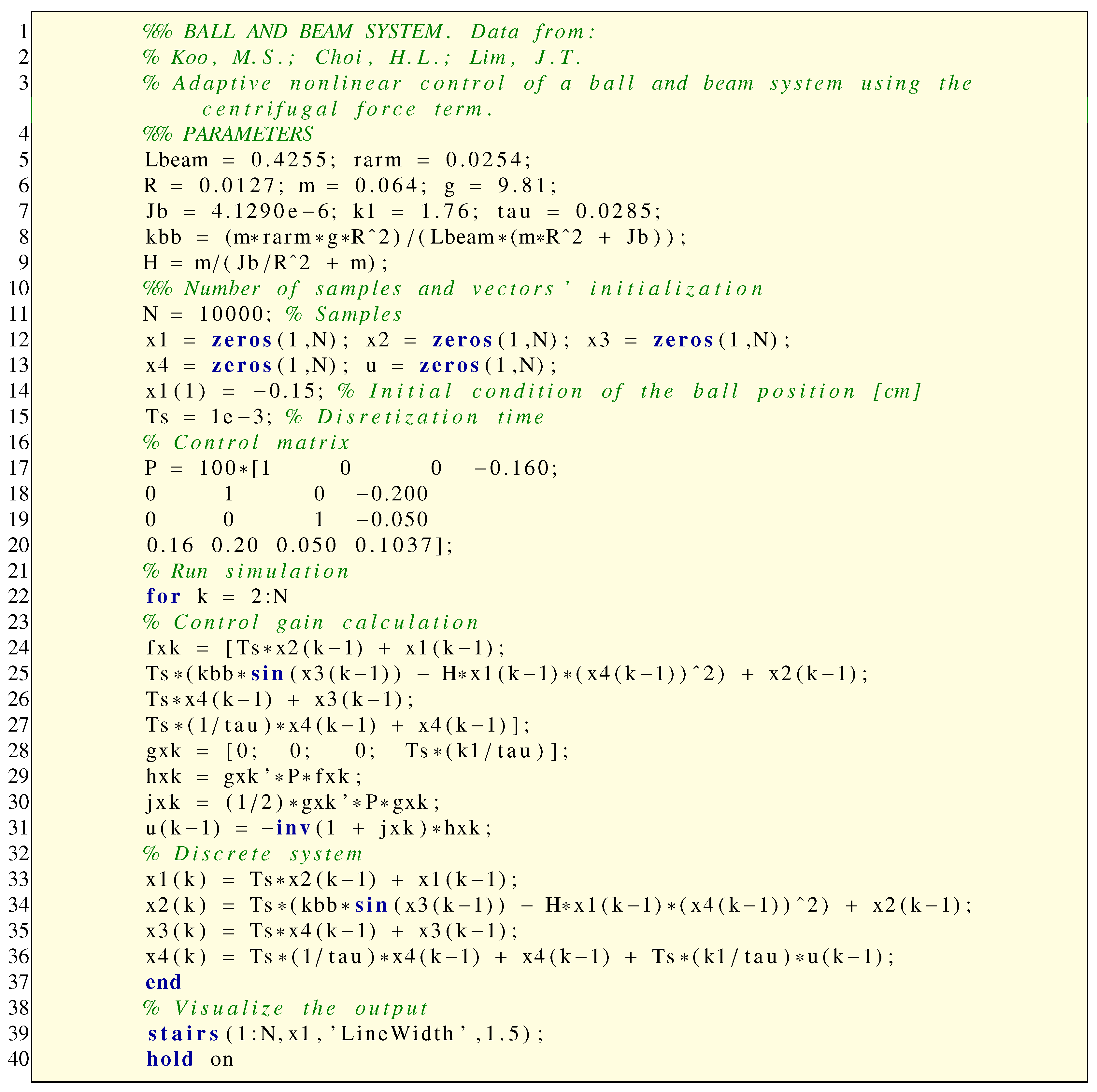
4. Numerical Validation

To demonstrate the effectiveness and robustness of the studied discrete-inverse optimal control for regulation variables in the ball and beam dynamical system, we use the parametric information reported in [2] as presented in

Table 1. Parameter information of the ball and beam system.

Parameter	Value	Unity
$L_{\mathrm{beam}}$	42.55	cm
$r_{\mathrm{arm}}$	2.54	cm
R	1.27	cm
m	64	mg
g	9.81	m/s2
$J_b$	4.1290$\times {10}^6$	kgm2
$k_1$	1.76	rad/sv
$\tau$	28.5	ms

.

With the parameters in Table 1, the coefficients $k_{bb}$ and h are 0.4183 and 0.7143, respectively. The discretization time ${\Delta }_k$ is assigned as $1\times {10}^{-3}$ s. To evaluate the dynamical performance of the proposed approach, the initial condition of the state variables is 15 cm for the ball position, i.e., for $x_{1_0}$, and zero for the rest of state variables.

The parametrization of the control design is based on the structure of the $\mathbf{P}$ matrix, which for the ball and beam system can take the following form,

$$\begin{array}{c}\hfill \mathbf{P}=\left[\begin{array}{cccc}r& 0& 0& j_1\\ 0& r& 0& j_2\\ 0& 0& r& j_3\\ -j_1& -j_2& -j_3& r\end{array}\right]\end{array}$$

(30)

note that $\mathbf{P}$ is a positive definite matrix, as it can be rewritten as $\mathbf{P}=\mathbf{R}+\mathbf{J}$, where $\mathbf{R}$ is a positive diagonal and $\mathbf{J}$ is skew-symmetry, for $r>0$ and $j_i>0$.

From the structure of the $\mathbf{P}$ matrix, we can observe that there exist four parameters that need to be adjusted to reach the desired dynamical performance, i.e., r and $j_1$ to $j_4$. Here, they are tuned via a trial and error procedure by running multiple simulations in the MATLAB/OCTAVE programming environments.

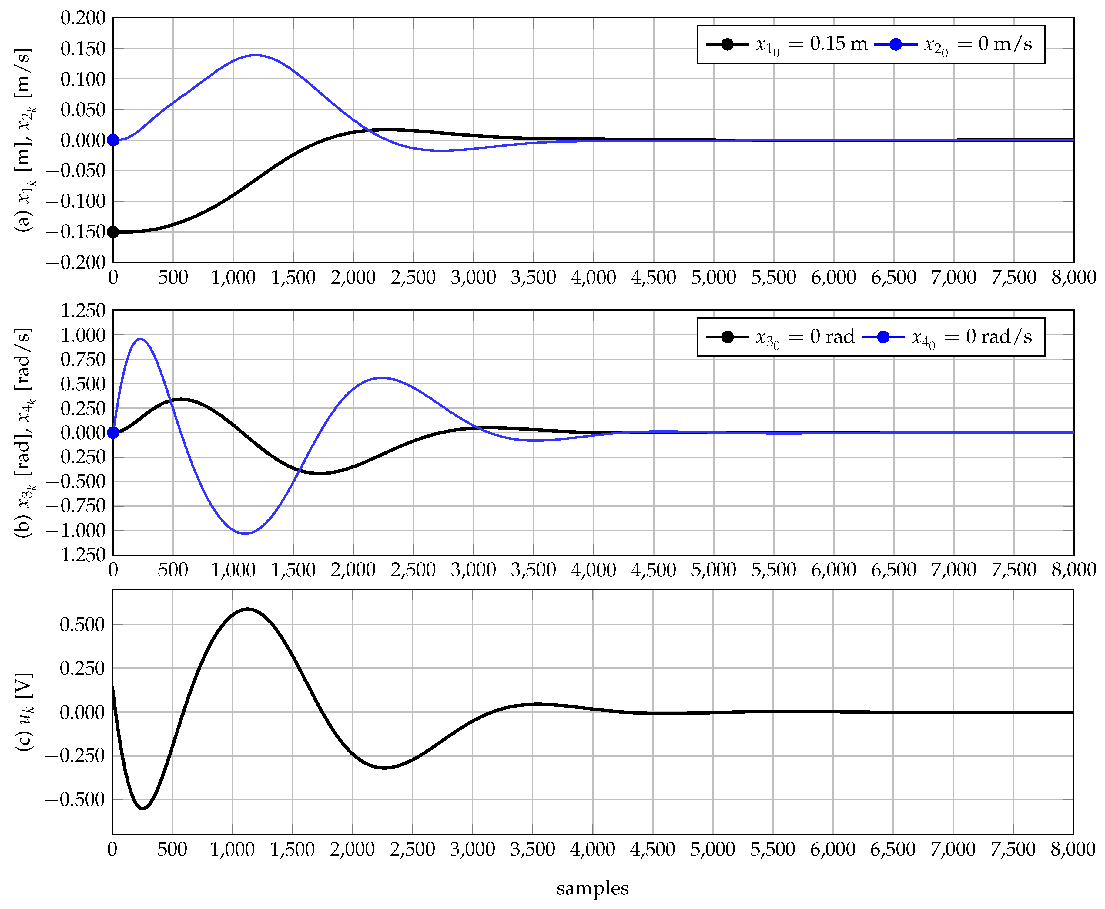
4.1. Regulation of the State Variables

In this simulation we present the ability of the proposed control to regulate all the state variables using the anti-symmetry nature of the $\mathbf{P}$ matrix, where the control gains were assigned as follows, $r=10.37$, $j_1=16$, $j_2=20$, and $j_3=5$.

Figure 2 presents the numerical behavior of each one of the state variables of the ball and beam system after its numerical simulations in MATLAB/OCTAVE software.

From Figure 2 we can observe the following.

✔

All the state variables are regulated when have passed 4000 samples, i.e., ~4 s, which implies that the discrete-inverse optimal control fulfill the control objective when the control input (28) is applied to the discrete equivalent system (3).

✔

The ball position exhibits a smooth dynamical behavior from the initial position (like a second-order system), i.e., $x_{1_0}=15$ cm, to the origin with a minimum overpass, which implies that the selection of the control gains was appropriate. Nevertheless, this behavior can also be improved (smoothing) if an optimization procedure over gains in $\mathbf{P}$ is made as recommended in [13].

✔

The control input $u_k$ presented in Figure 2c reaches the zero value when all the state variables are in the origin of coordinates, which is a natural behavior as it is a nonlinear function of all these variables working as a proportional controller that reduces its amplitude when the regulated variables are near to the origin of coordinates.

It is worth mentioning that the proposed controller can regulate all the state variables for the ball and beam system even if this system is strong nonlinear with unique control input and four dynamical equations with a basic implementation in the discrete domain. Figure 3 provides the MATLAB/OCTAVE code implementation that generates all the dynamical behaviors reported in Figure 2.

Note that the main idea of providing the MATLAB/OCTAVE code in Figure 3 is the possibility of using it for possible comparisons in future works by engineering students and researches related to nonlinear control areas.

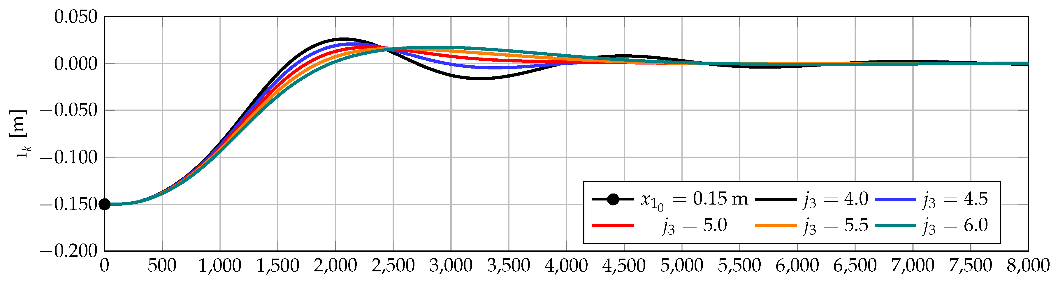
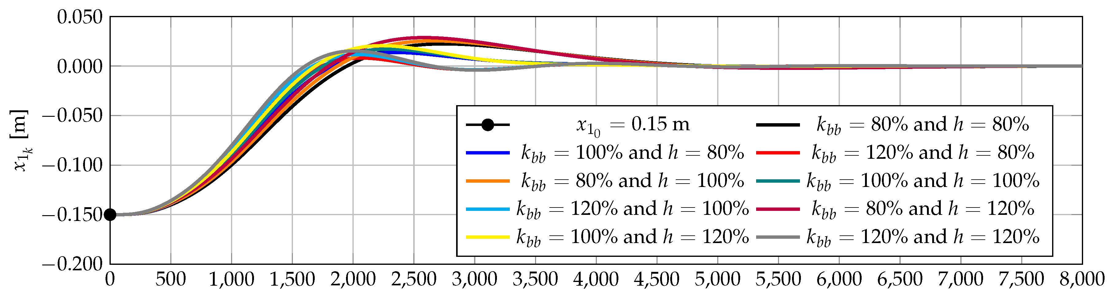
4.2. Dynamical Performance for Different Control Gains

This subsection explores the effect that has the variations in the control gains in the matrix $\mathbf{P}$ regarding the dynamical performance of the ball position. Figure 4 presents some dynamical outputs of the ball position for variations in the control gain $j_3$. These variations begin with $j_3=4$ and ends with $j_3=6$.

The results in Figure 4 demonstrate that the dynamical behavior of the ball position is strongly related to the control gain $j_3$, as values of approximately 4 produce higher oscillations in its position that vanish after 6500 samples, i.e., 6.5 s approximately. When this gain increases until 6, the system has low oscillations, and the settling time is ~4.5 s.

It is important to point out that similar behaviors on the ball position can be reached if r or $j_2$ are also modified because, as aforementioned, the control input (28) is a nonlinear function of the state variables, which implies that these allow governing the closed-loop behavior of the ball and beam system.

4.3. Effect of the Parameter Variations

To evaluate the ability of the proposed discrete-inverse optimal control to deal with parametric uncertainties, we consider that parameters h and $k_{bb}$ have a $20\%$ of error in their calculations. This implies that in the dynamical model, these parameters are different from the user to design the controller. Figure 5 presents the dynamical performance of the ball position for different combinations of the parameters h and $k_{bb}$.

From Figure 5, we can observe that the variation in the parameters associated with the physical quantities of the ball and beam system, i.e., h and $k_{bb}$, has effects on the dynamical behavior of the ball position. Nevertheless, this does not compromise the stability properties ensured by the discrete-inverse optimal control law proposed in this research. In addition, from this simulation, it is possible to note that the setting time remains constant at approximately 4.5 s, which is the same time reported when all the parameters are entirely known. This confirms the robustness of the proposed control approach to possible parametric uncertainties.

5. Conclusions and Future Works

In this paper, the nonlinear discrete-inverse optimal control approach to regulate all the state variables in the discrete version of the ball and beam system was proposed. Numerical results confirm that the proposed controller allows guaranteeing passivity, stability, and optimally properties during closed-loop operation. In addition, numerical simulations show that the dynamical behavior of the system is highly dependent on the control gains contained in the $\mathbf{P}$ matrix as one or more of then can produce similar dynamical performances with small oscillations around the origin of coordinates. The control design robustness was tested by varying the parameters $k_{bb}$ and h from 80 % to 120% of their nominal rates, where simulations demonstrate that in all of these cases the setting time remains constant at approximately 4.5 s with smooth oscillations around the control objective, i.e., the origin of coordinates.

As future works it will be possible to develop the following. (i) The experimental validation of the discrete-inverse optimal control and their comparisons with nonlinear control methodologies, (ii) the application of the interconnection and damping assignment control to regulate all the state variables by taking advantage on the open-loop model of the ball and beam via Hamiltonian functions, and (iii) the extension of the proposed discrete-inverse optimal control to the four-order model of the synchronous machine system to regulate the angular deviation when short-circuit scenarios appear in the power system.

References

1. Kagami, R.M.; da Costa, G.K.; Uhlmann, T.S.; Mendes, L.A.; Freire, R.Z. A Generic WebLab Control Tuning Experience Using the Ball and Beam Process and Multiobjective Optimization Approach. Information 2020, 11, 132. [Google Scholar] [CrossRef] [Green Version]
2. Koo, M.S.; Choi, H.L.; Lim, J.T. Adaptive nonlinear control of a ball and beam system using the centrifugal force term. Int. J. Innov. Comput. Inf. Control 2012, 8, 5999–6009. [Google Scholar]
3. Ye, H.; Gui, W.; Yang, C. Novel Stabilization Designs for the Ball-and-Beam System. IFAC Proc. Vol. 2011, 44, 8468–8472. [Google Scholar] [CrossRef] [Green Version]
4. Rahmat, M.F.; Wahid, H.; Wahab, N.A. Application of intelligent controller in a ball and beam control system. Int. J. Smart Sens. Intell. Syst. 2010, 3, 45–60. [Google Scholar] [CrossRef] [Green Version]
5. Meenakshipriya, B.; Kalpana, K. Modelling and Control of Ball and Beam System using Coefficient Diagram Method (CDM) based PID controller. IFAC Proc. Vol. 2014, 47, 620–626. [Google Scholar] [CrossRef]
6. Ding, M.; Liu, B.; Wang, L. Position control for ball and beam system based on active disturbance rejection control. Syst. Sci. Control. Eng. 2019, 7, 97–108. [Google Scholar] [CrossRef] [Green Version]
7. Qi, X.; Li, J.; Xia, Y.; Wan, H. On stability for sampled-data nonlinear ADRC-based control system with application to the ball-beam problem. J. Franklin Inst. 2018, 355, 8537–8553. [Google Scholar] [CrossRef]
8. Chen, C.C.; Chien, T.L.; Wei, C.L. Application of Feedback Linearization to Tracking and Almost Disturbance Decoupling Control of the AMIRA Ball and Beam System. J. Optim. Theory Appl. 2004, 121, 279–300. [Google Scholar] [CrossRef] [Green Version]
9. Aguilar-Ibañez, C.; Suarez-Castanon, M.S.; de Jesús Rubio, J. Stabilization of the Ball on the Beam System by Means of the Inverse Lyapunov Approach. Math. Probl. Eng. 2012, 2012, 1–13. [Google Scholar] [CrossRef]
10. Li, E.; Liang, Z.Z.; Hou, Z.G.; Tan, M. Energy-based balance control approach to the ball and beam system. Int. J. Control 2009, 82, 981–992. [Google Scholar] [CrossRef]
11. Kelly, R.; Sandoval, J.; Santibáñez, V. A Novel Estimate of The Domain of Attraction of an IDA-PBC of a Ball and Beam System. IFAC Proc. Vol. 2011, 44, 8463–8467. [Google Scholar] [CrossRef] [Green Version]
12. Chang, Y.H.; Chang, C.W.; Tao, C.W.; Lin, H.W.; Taur, J.S. Fuzzy sliding-mode control for ball and beam system with fuzzy ant colony optimization. Expert Syst. Appl. 2012, 39, 3624–3633. [Google Scholar] [CrossRef]
13. Castillo, O.; Lizárraga, E.; Soria, J.; Melin, P.; Valdez, F. New approach using ant colony optimization with ant set partition for fuzzy control design applied to the ball and beam system. Inf. Sci. 2015, 294, 203–215. [Google Scholar] [CrossRef]
14. Zavala, S.J.; Yu, W.; Li, X. Synchronization of two ball and beam systems with neural compensation. IFAC Proc. Vol. 2008, 41, 12781–12786. [Google Scholar] [CrossRef]
15. Ornelas, F.; Loukianov, A.G.; Sanchez, E.N. Discrete-time Robust Inverse Optimal Control for a Class of Nonlinear Systems. IFAC Proc. Vol. 2011, 44, 8595–8600. [Google Scholar] [CrossRef] [Green Version]
16. Atkinson, C.; Osseiran, A. Discrete-space time-fractional processes. Fract. Calc. Appl. Anal. 2011, 14. [Google Scholar] [CrossRef]
17. Carrasco-Gutierrez, C.E.; Sosa, W. A discrete dynamical system and its applications. Pesqui. Oper. 2019, 39, 457–469. [Google Scholar] [CrossRef]
18. Sanchez, E.N.; Ornelas-Tellez, F. Discrete-Time Inverse Optimal Control for Nonlinear Systems; CRC Press Taylor and Francis Group: Boca Raton, FL, USA, 2017. [Google Scholar]
19. Galor, O. Discrete Dynamical Systems; Springer: Berlin/Heidelberg, Germany, 2007. [Google Scholar] [CrossRef]
20. Gil-González, W.; Serra, F.M.; Montoya, O.D.; Ramírez, C.A.; Orozco-Henao, C. Direct Power Compensation in AC Distribution Networks with SCES Systems via PI-PBC Approach. Symmetry 2020, 12, 666. [Google Scholar] [CrossRef] [Green Version]
21. la Sen, M.D. On the Passivity and Positivity Properties in Dynamic Systems: Their Achievement under Control Laws and Their Maintenance under Parameterizations Switching. J. Math. 2018, 2018, 1–16. [Google Scholar] [CrossRef] [Green Version]
22. Navarro-López, E.; Fossas-Colet, E. Dissipativity, passivity, and feedback passivity in the nonlinear discrete-time setting. IFAC Proc. Vol. 2002, 35, 257–262. [Google Scholar] [CrossRef] [Green Version]
Figure 1. Schematic representation of the ball and beam dynamical system.
Symmetry 12 01359 g001
Figure 2. Time-domain behavior of the state variables and control input in the ball and beam system: (a) position and and speed of the ball, (b) angular position and angular speed of the beam, and (c) control input.
Symmetry 12 01359 g002
Figure 3. MATLAB/OCTAVE implementation of the inverse optimal controller for the ball and beam system.
Symmetry 12 01359 g003
Figure 4. Dynamical behavior of the ball position for different values of the gain j 3 .
Symmetry 12 01359 g004
Figure 5. Dynamical behavior of the ball position when parametric variations are experimented in h and k b b parameters.
Symmetry 12 01359 g005