Simulation of Boiling Heat Transfer at Different Reduced Temperatures with an Improved Pseudopotential Lattice Boltzmann Method

 , , , , and
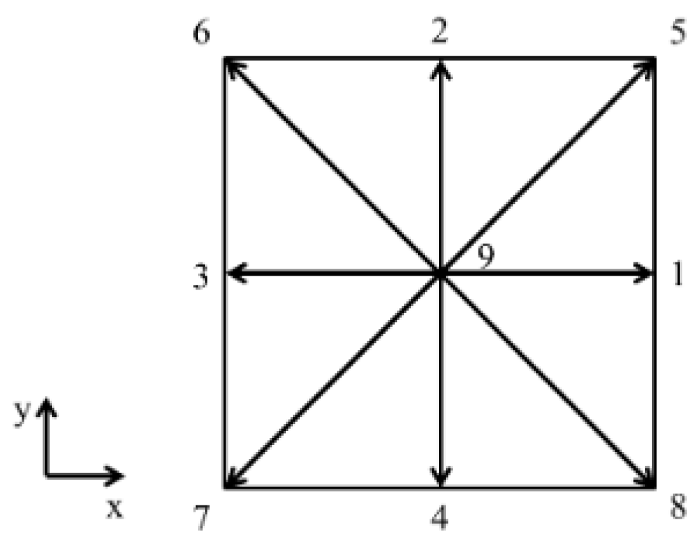
Abstract
:1. Introduction
2. Hydrodynamic Model: Improved Pseudopotential Lattice Boltzmann Method
3. Modeling the Energy Conservation Equation
4. Results and Discussion
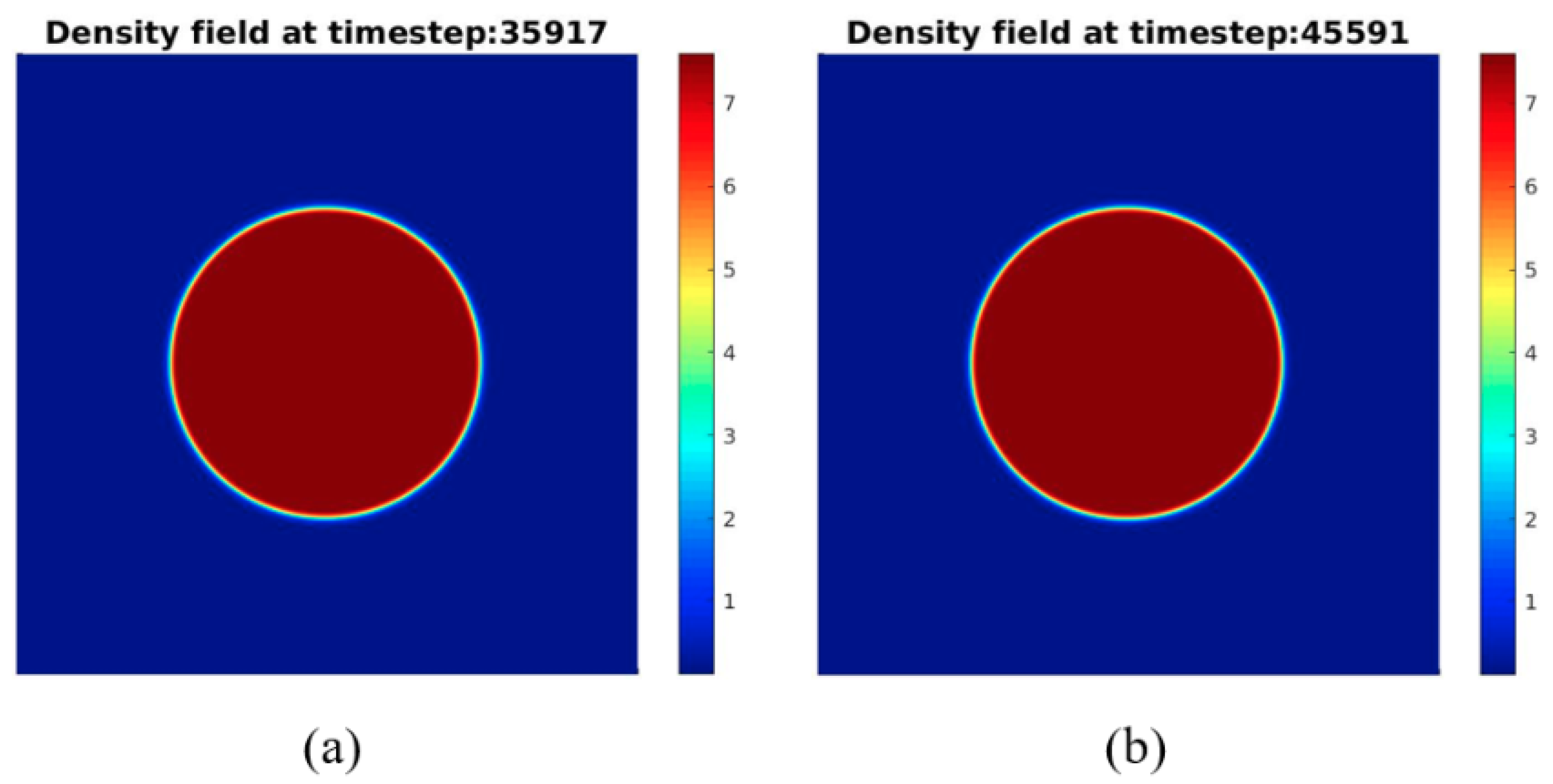
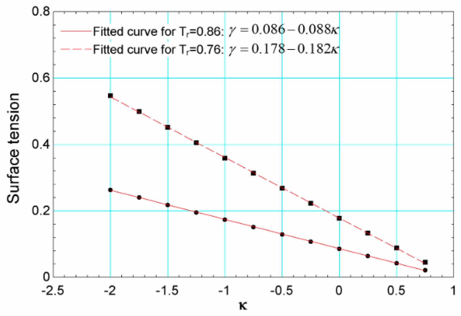
4.1. Computation of the Surface Tension: Young–Laplace Test
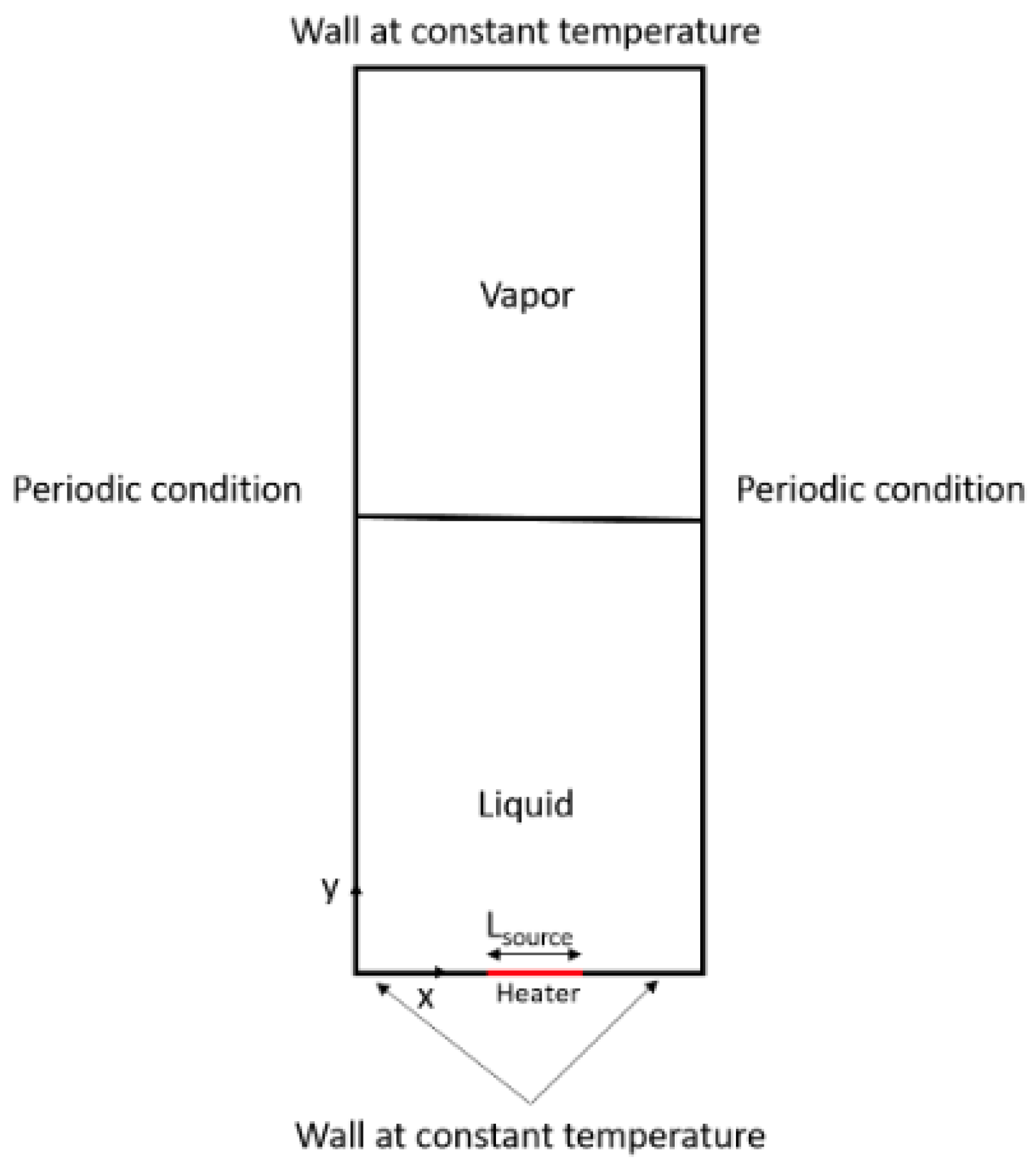
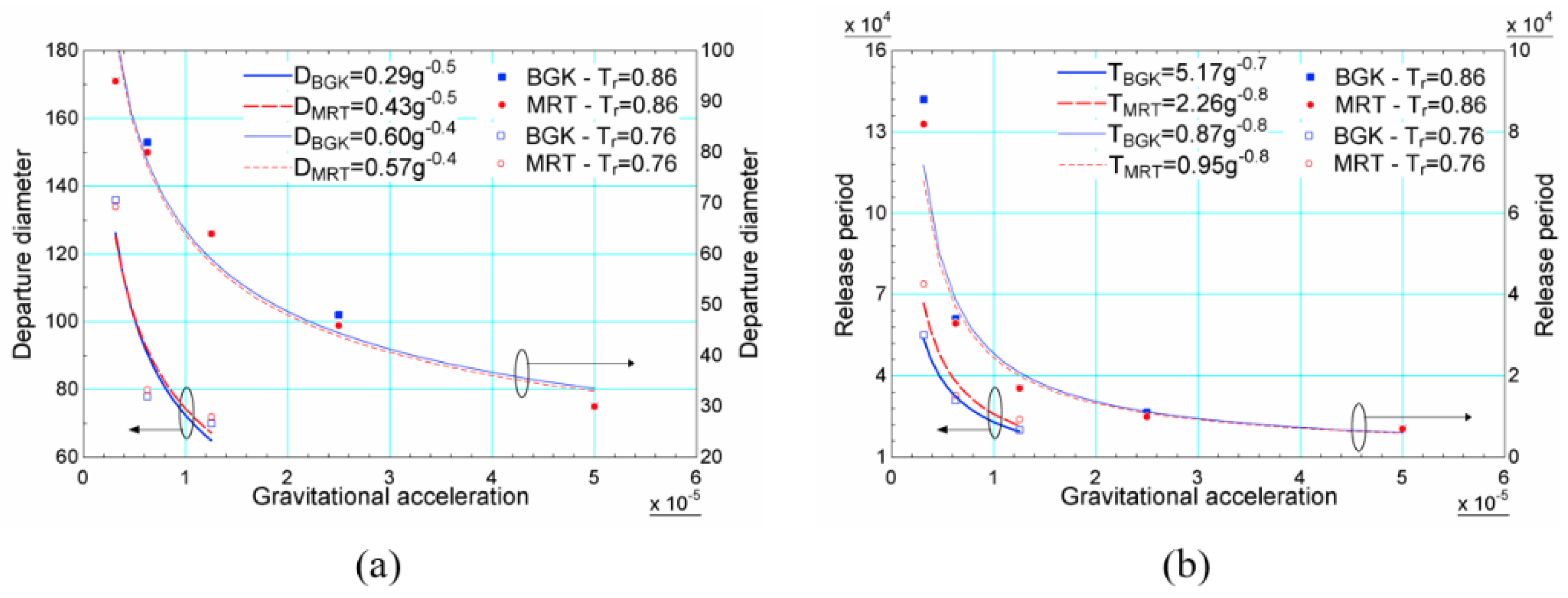
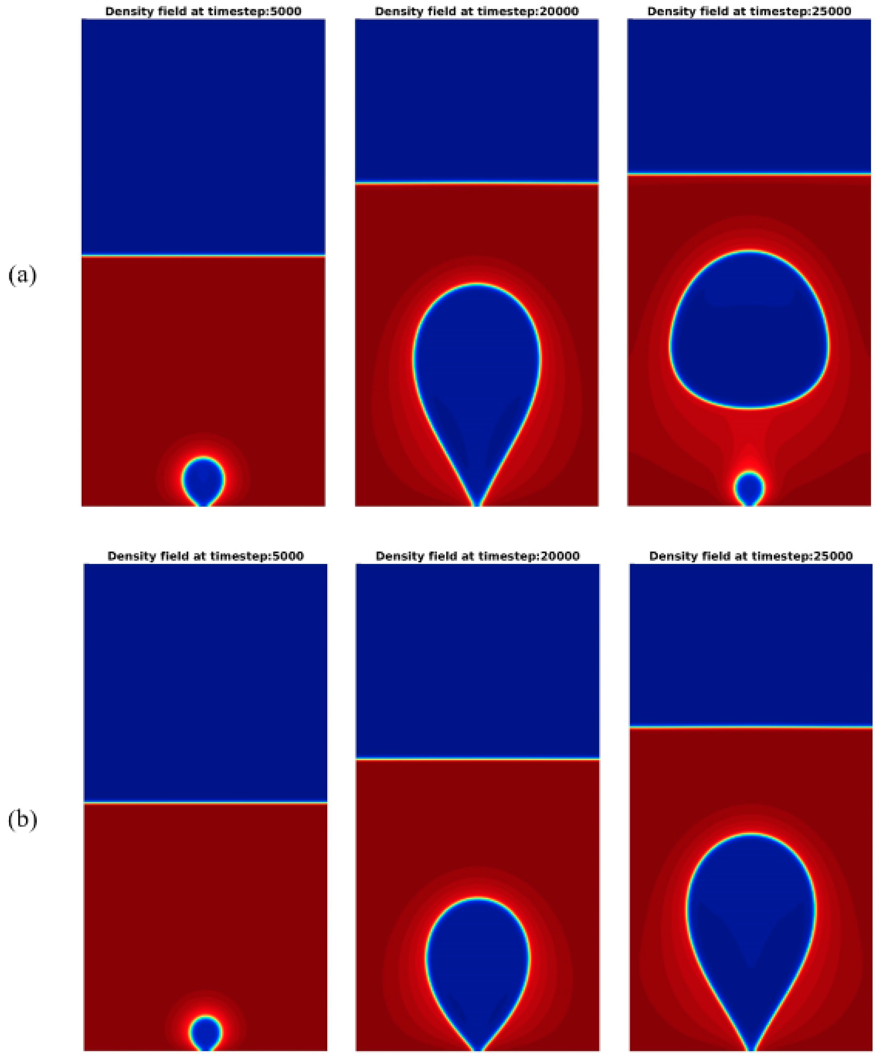
4.2. Single Bubble Nucleation: Bubble Departure Diameter and Release Period versus Gravitational Acceleration
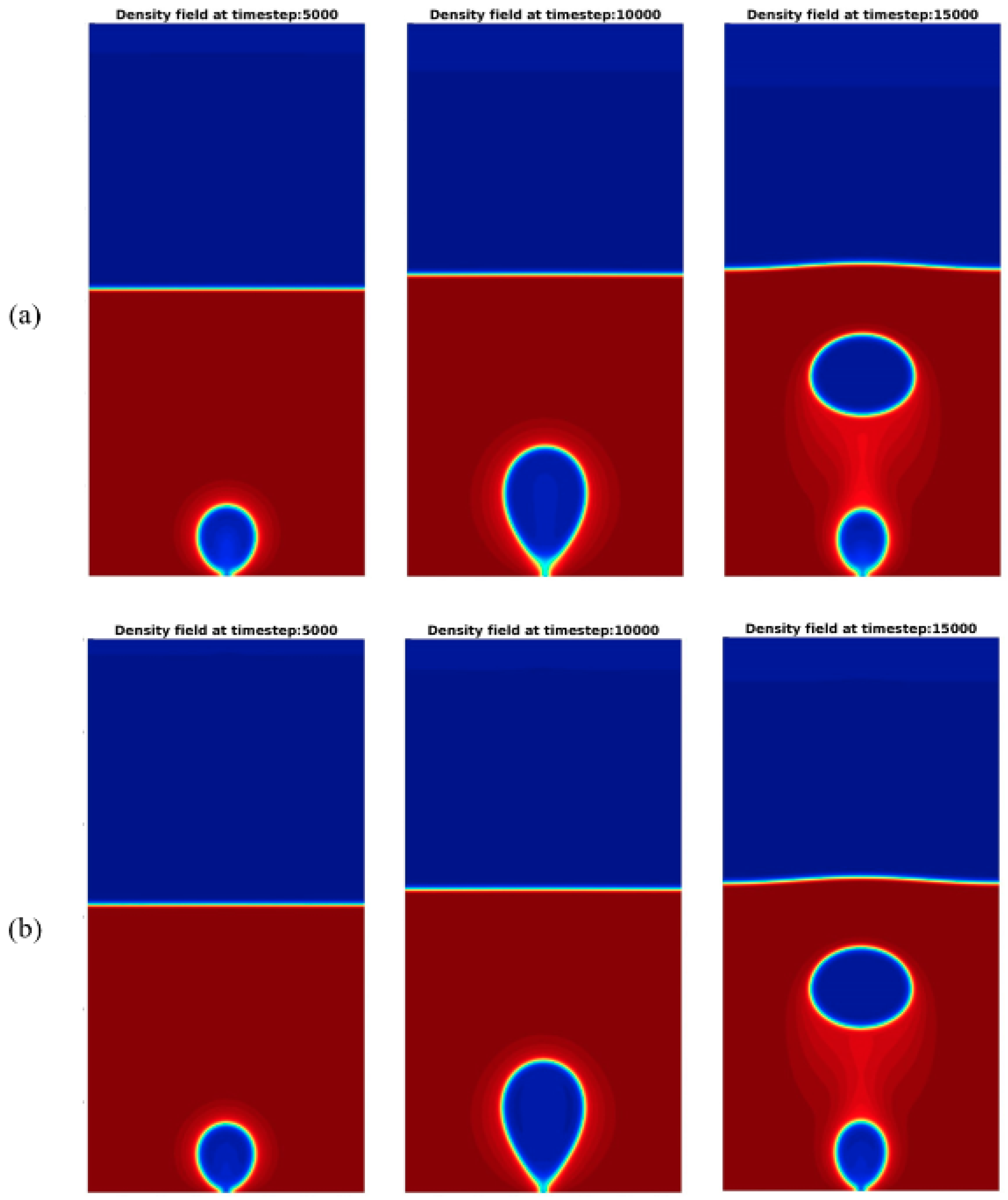
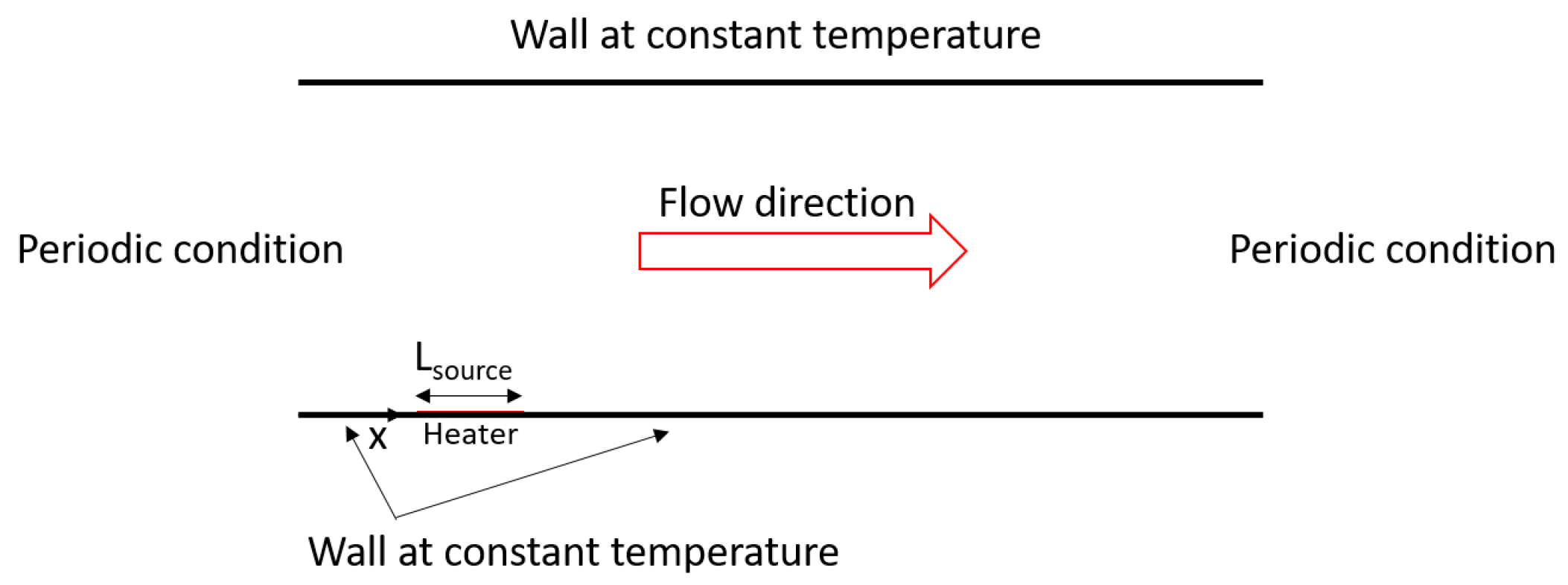
4.3. Single Bubble Nucleation under Forced Convection
5. Conclusions
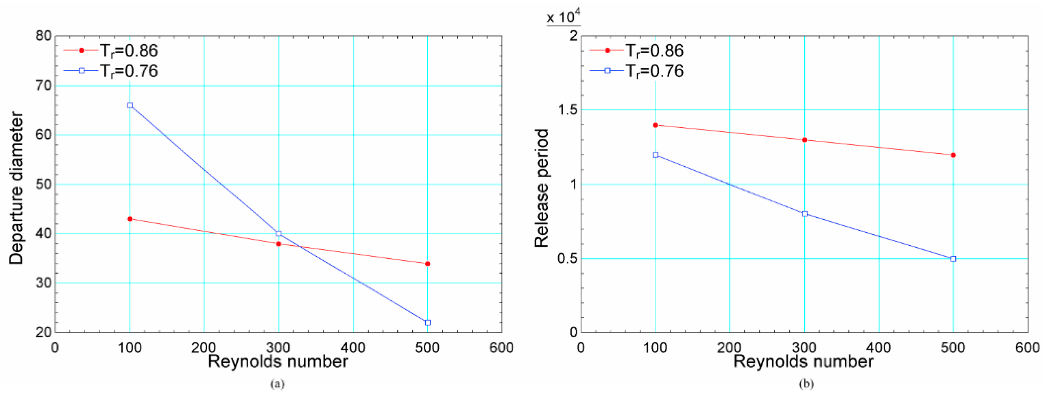
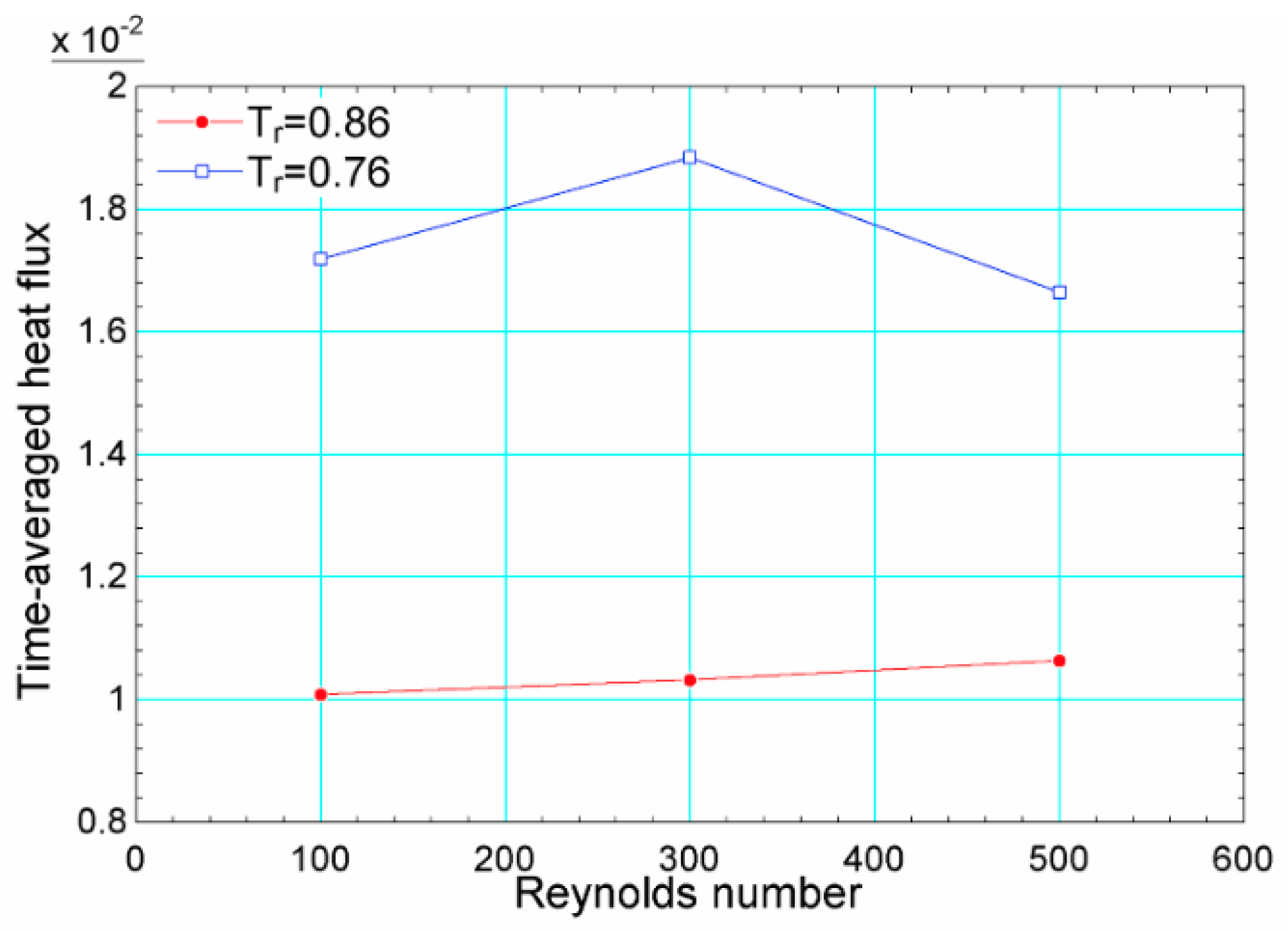
- The comparison between the results for different reduced temperatures revealed that the decrease of the reduced temperature results in bubbles with higher departure diameter and higher release period for the pool boiling case. This behavior is in accordance with boiling heat transfer theory. In the case of flow boiling, the departure diameter, reduces as the Reynolds number is increased, indicating that this quantity is a strong function of the drag force.
- In the pool boiling simulations, at both reduced temperatures, and , a reasonable agreement is observed for the departure diameter regarding the results obtained with both simulation models. The release period also showed good agreement, presenting some discrepancies for the lowest gravitational acceleration, namely . This might suggest an influence of the forcing scheme used for the model with the BGK collision operator over the numerical results. This observation is based on the fact that models with the BGK collision operator use a single relaxation time related to the assumed kinematic viscosity. For the considered forcing scheme, this affects in more extend the coexistence densities at large densities ratios. It is a fact that even in single-phase flow simulations models with the BGK collision operator present less numerical stability than those with the models with the MRT collision operator [29].
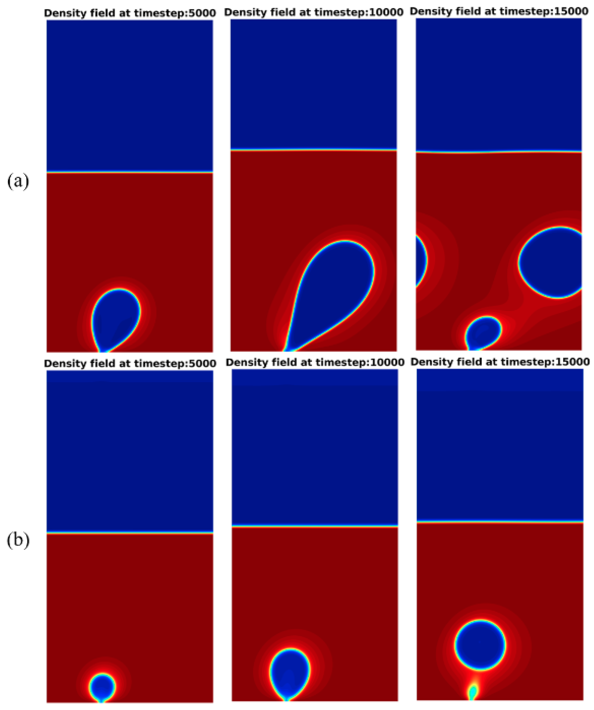
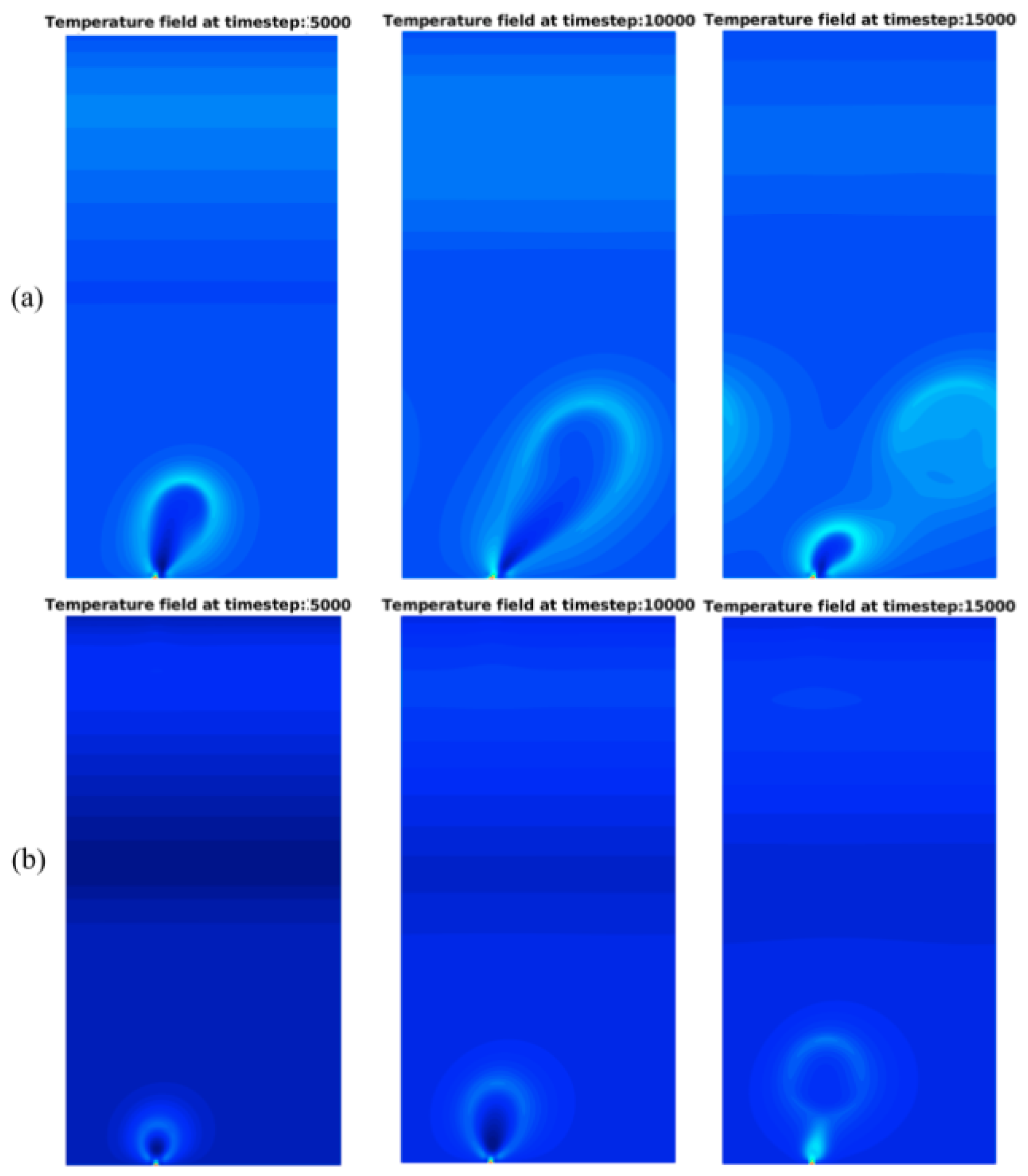
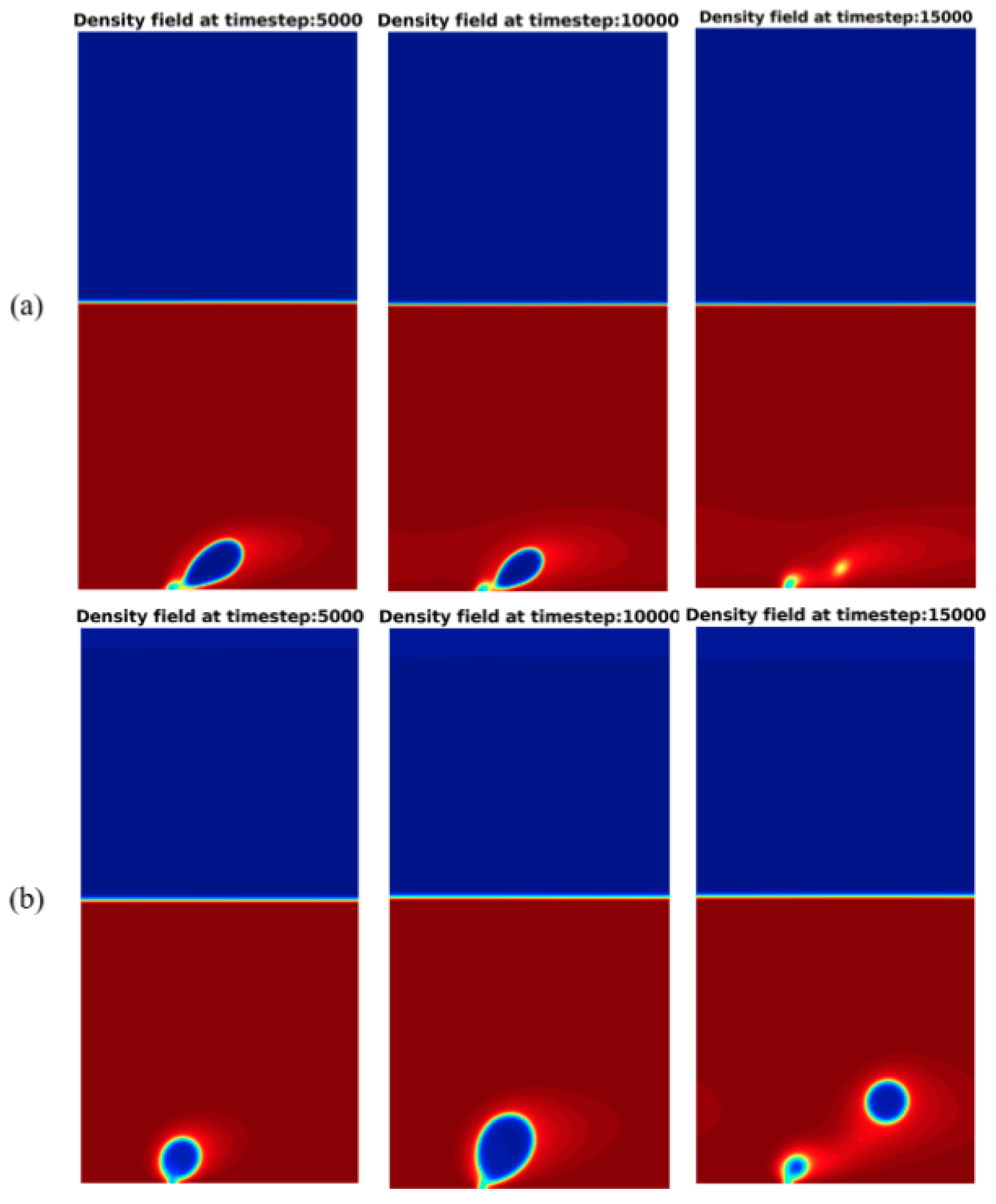
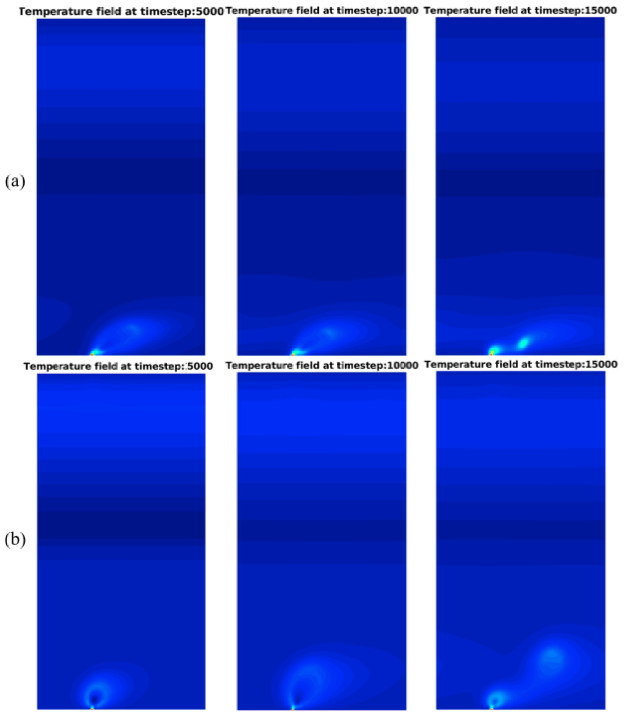
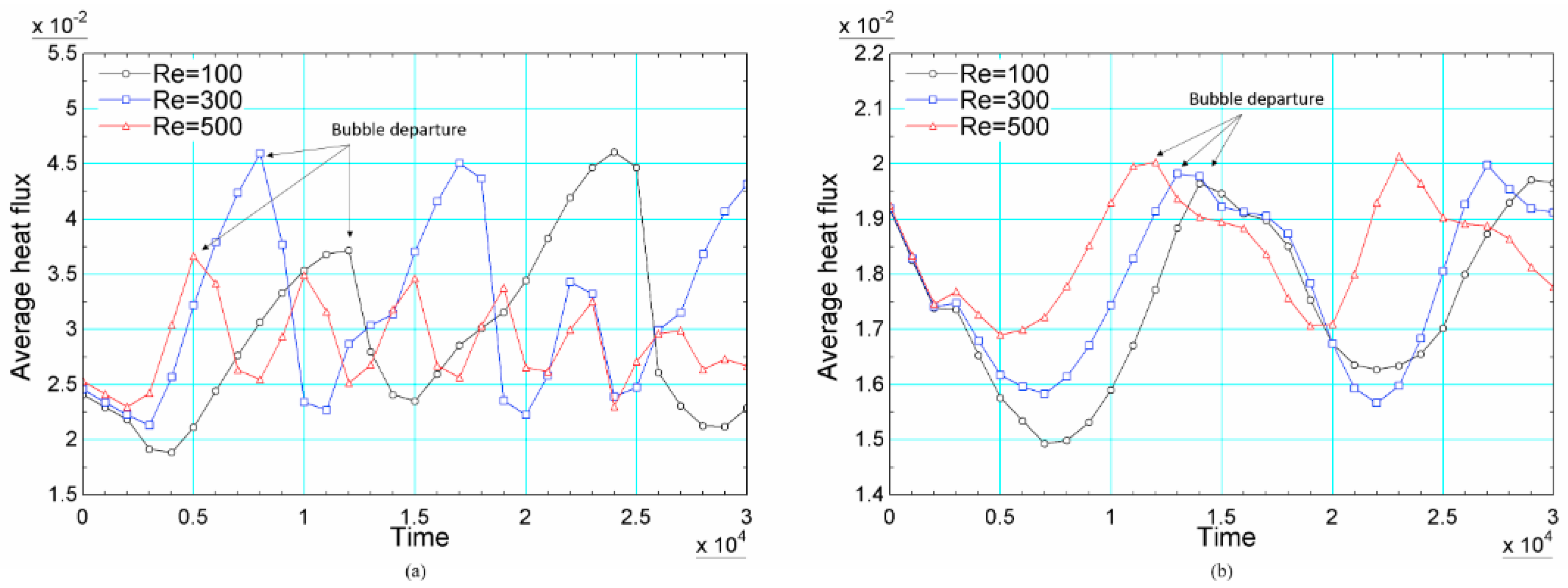
- For pool boiling and flow boiling simulations, the space-averaged heat flux is an important quantity. for the pool boiling simulations, the expansion and rewetting stages can be identified. For the flow boiling, the release period of the departure bubbles can be identified by the heat flux peak. For flow boiling simulations at both reduced temperature, the periodic behavior of the heat flux is observed for all simulated Reynolds number. At and , the effect of the Reynolds number is to anticipate the bubble departure.
- The pool boiling results showed that the gravitational acceleration plays a very important role on the LBM numerical stability for medium to lower reduced temperatures. The same behavior can be attributed to the flow boiling problem. This behavior is present even when the MRT model is used. In order to avoid these numerical instabilities, small values of gravitational acceleration should be used. This introduces a question regarding the simulation of real boiling process for medium to lower reduced temperatures ().The use of very small values of gravitational acceleration can produce difficulties in fitting the LBM simulations into the desired limits of dimensionless numbers necessary to simulate a particular heat transfer phase-change process, i.e., the Grashof and Bond numbers. Further investigations are under development to address this issue.
Author Contributions
Funding
Conflicts of Interest
Abbreviations
| LBM | Lattice Boltzmann Method |
| BGK | Bhatnagar–Gross–Krook |
| MRT | Multiple-Relaxation-Time |
References
- Luo, K.H.; Xia, J.; Monaco, E. Multiscale modeling of multiphase flow with complex interactions. J. Multiscale Model. 2009, 1, 125–156. [Google Scholar] [CrossRef]
- Grunau, D.; Chen, S.; Eggert, K. A lattice Boltzmann model for multiphase fluid flows. Phys. Fluids A Fluid Dyn. 1993, 5, 2557–2562. [Google Scholar] [CrossRef] [Green Version]
- D’Ortona, U.; Salin, D.; Cieplak, M.; Rybka, R.B.; Banavar, J.R. Two-color nonlinear Boltzmann cellular automata: Surface tension and wetting. Phys. Rev. E 1995, 51, 3718–3728. [Google Scholar] [CrossRef]
- Lishchuk, S.V.; Care, C.M.; Halliday, I. Lattice Boltzmann algorithm for surface tension with greatly reduced microcurrents. Phys. Rev. E 2003, 67, 036701. [Google Scholar] [CrossRef]
- Reis, T.; Phillips, T.N. Lattice Boltzmann model for simulating immiscible two-phase flows. J. Phys. A Math. Theor. 2007, 40, 4033. [Google Scholar] [CrossRef]
- Park, S.D.; Kim, J.H.; Bang, I.C. Experimental study on a novel liquid metal fin concept preventing boiling critical heat flux for advanced nuclear power reactors. Appl. Therm. Eng. 2016, 98, 743–755. [Google Scholar] [CrossRef]
- El-Genk, M.S. Immersion cooling nucleate boiling of high power computer chips. Energy Convers. Manag. 2012, 53, 205–218. [Google Scholar] [CrossRef]
- Pulvirenti, B.; Matalone, A.; Barucca, U. Boiling heat transfer in narrow channels with offset strip fins: Application to electronic chipsets cooling. Appl. Therm. Eng. 2010, 30, 2138–2145. [Google Scholar] [CrossRef] [Green Version]
- Alvariño, P.F.; Simón, M.L.S.; dos Santos Guzella, M.; Paz, J.M.A.; Jabardo, J.M.S.; Gómez, L.C. Experimental investigation of the CHF of HFE-7100 under pool boiling conditions on differently roughened surfaces. Int. J. Heat Mass Transf. 2019, 139, 269–279. [Google Scholar] [CrossRef]
- Zhang, R.; Chen, H. Lattice Boltzmann method for simulations of liquid-vapor thermal flows. Phys. Rev. E 2003, 67, 066711. [Google Scholar] [CrossRef] [Green Version]
- Hazi, G.; Markus, A. On the bubble departure diameter and release frequency based on numerical simulation results. Int. J. Heat Mass Transf. 2009, 52, 1472–1480. [Google Scholar] [CrossRef]
- Gong, S.; Cheng, P. A lattice Boltzmann method for simulation of liquid–vapor phase-change heat transfer. Int. J. Heat Mass Transf. 2012, 55, 4923–4927. [Google Scholar] [CrossRef]
- Fritz, W. Berechnung des maximalvolumes von dampfblasen. Physik. Zeitschr 1935, 36, 379–384. [Google Scholar]
- Gong, S.; Cheng, P. Lattice Boltzmann simulations for surface wettability effects in saturated pool boiling heat transfer. Int. J. Heat Mass Transf. 2015, 85, 635–646. [Google Scholar] [CrossRef]
- Gong, S.; Cheng, P. Numerical simulation of pool boiling heat transfer on smooth surfaces with mixed wettability by lattice Boltzmann method. Int. J. Heat Mass Transf. 2015, 80, 206–216. [Google Scholar] [CrossRef]
- Gong, S.; Cheng, P.; Quan, X. Two-dimensional mesoscale simulations of saturated pool boiling from rough surfaces. Part I: Bubble nucleation in a single cavity at low superheats. Int. J. Heat Mass Transf. 2016, 100, 927–937. [Google Scholar] [CrossRef]
- Gong, S.; Cheng, P. Two-dimensional mesoscale simulations of saturated pool boiling from rough surfaces. Part II: Bubble interactions above multi-cavities. Int. J. Heat Mass Transf. 2016, 100, 938–948. [Google Scholar] [CrossRef]
- Li, Q.; Zhou, P.; Yan, H.J. Improved thermal lattice Boltzmann model for simulation of liquid-vapor phase change. Phys. Rev. E 2017, 96, 063303. [Google Scholar] [CrossRef] [Green Version]
- Gong, S.; Cheng, P. Direct numerical simulations of pool boiling curves including heater’s thermal responses and the effect of vapor phase’s thermal conductivity. Int. Commun. Heat Mass Transf. 2017, 87, 61–71. [Google Scholar] [CrossRef]
- Li, Q.; Kang, Q.J.; Francois, M.M.; He, Y.L.; Luo, K.H. Lattice Boltzmann modeling of boiling heat transfer: The boiling curve and the effects of wettability. Int. J. Heat Mass Transf. 2015, 85, 787–796. [Google Scholar] [CrossRef] [Green Version]
- Hu, A.; Liu, D. 2D Simulation of boiling heat transfer on the wall with an improved hybrid lattice Boltzmann model. Appl. Therm. Eng. 2019, 159, 113788. [Google Scholar] [CrossRef]
- Chang, X.; Huang, H.; Cheng, Y.P.; Lu, X.Y. Lattice Boltzmann study of pool boiling heat transfer enhancement on structured surfaces. Int. J. Heat Mass Transf. 2019, 139, 588–599. [Google Scholar] [CrossRef]
- Zhang, L.; Wang, T.; Kim, S.; Jiang, Y. The effects of wall superheat and surface wettability on nucleation site interactions during boiling. Int. J. Heat Mass Transf. 2020, 146, 118820. [Google Scholar] [CrossRef]
- Zhang, L.; Shoji, M. Nucleation site interaction in pool boiling on the artificial surface. Int. J. Heat Mass Transf. 2003, 46, 513–522. [Google Scholar] [CrossRef]
- Zhang, L.; Shoji, M. Studies of boiling chaos: A review. Int. J. Heat Mass Transf. 2004, 47, 1105–1128. [Google Scholar]
- Hutter, C.; Sefiane, K.; Karayiannis, T.; Walton, A.; Nelson, R.; Kenning, D. Nucleation site interaction between artificial cavities during nucleate pool boiling on silicon with integrated micro-heater and temperature microsensors. Int. J. Heat Mass Transf. 2012, 55, 2769–2778. [Google Scholar] [CrossRef]
- Li, Q.; Luo, K.H.; Li, X.J. Forcing scheme in pseudopotential lattice Boltzmann model for multiphase flows. Phys. Rev. E 2012, 86, 016709. [Google Scholar] [CrossRef] [PubMed] [Green Version]
- Li, Q.; Luo, K.H.; Li, X.J. Lattice Boltzmann modeling of multiphase flows at large density ratio with an improved pseudopotential model. Phys. Rev. E 2013, 87, 053301. [Google Scholar] [CrossRef] [Green Version]
- Krüger, T.; Kusumaatmaja, H.; Kuzmin, A.; Shardt, O.; Silva, G.; Viggen, E.M. The Lattice Boltzmann Method; Springer: Cham, Switzerland, 2017. [Google Scholar]
- Bhatnagar, P.L.; Gross, E.P.; Krook, M. A Model for Collision Processes in Gases. I. Small Amplitude Processes in Charged and Neutral One-Component Systems. Phys. Rev. E 1954, 94, 511–525. [Google Scholar] [CrossRef]
- Shan, X.; Chen, H. Lattice Boltzmann model for simulating flows with multiple phases and components. Phys. Rev. E 1993, 47, 1815. [Google Scholar] [CrossRef] [Green Version]
- Yuan, P.; Schaefer, L. Equations of state in a lattice Boltzmann model. Phys. Fluids 2006, 18, 042101. [Google Scholar] [CrossRef]
- Guo, Z.; Zheng, C.; Shi, B. Discrete lattice effects on the forcing term in the lattice Boltzmann method. Phys. Rev. E 2002, 65, 046308. [Google Scholar] [CrossRef]
- Higuera, F.J.; Jiménez, J. Boltzmann approach to lattice gas simulations. Europhys. Lett. 1989, 9, 663. [Google Scholar] [CrossRef]
- Higuera, F.J.; Succi, S.; Benzi, R. Lattice gas dynamics with enhanced collisions. Europhys. Lett. 1989, 9, 345. [Google Scholar] [CrossRef]
- Li, Q.; Luo, K.H.; He, Y.; Gao, Y.J.; Tao, W.Q. Coupling lattice Boltzmann model for simulation of thermal flows on standard lattices. Phys. Rev. E 2012, 85, 016710. [Google Scholar] [CrossRef] [PubMed] [Green Version]
- Lallemand, P.; Luo, L.S. Theory of the lattice Boltzmann method: Dispersion, dissipation, isotropy, Galilean invariance, and stability. Phys. Rev. E 2000, 61, 6546. [Google Scholar] [CrossRef] [PubMed] [Green Version]
- Li, Q.; Luo, K.H. Achieving tunable surface tension in the pseudopotential lattice Boltzmann modeling of multiphase flows. Phys. Rev. E 2013, 88, 053307. [Google Scholar] [CrossRef] [PubMed] [Green Version]
- Anderson, D.M.; McFadden, G.B.; Wheeler, A.A. Diffuse-interface methods in fluid mechanics. Annu. Rev. Fluid Mech. 1998, 30, 139–165. [Google Scholar] [CrossRef] [Green Version]
- Lee, T.; Lin, C.L. A stable discretization of the lattice Boltzmann equation for simulation of incompressible two-phase flows at high density ratio. J. Comput. Phys. 2005, 206, 16–47. [Google Scholar] [CrossRef]
- Huang, H.; Krafczyk, M.; Lu, X. Forcing term in single-phase and Shan-Chen-type multiphase lattice Boltzmann models. Phys. Rev. E 2011, 84, 046710. [Google Scholar] [CrossRef] [Green Version]
- Zou, Q.; He, X. On pressure and velocity boundary conditions for the lattice Boltzmann BGK model. Phys. Fluids 1997, 9, 1591–1598. [Google Scholar] [CrossRef] [Green Version]
- Zuber, N. Nucleate boiling. The region of isolated bubbles and the similarity with natural convection. Int. J. Heat Mass Transf. 1963, 6, 53–78. [Google Scholar] [CrossRef]
- Li, Q.; Luo, K.H.; Kang, Q.J.; He, Y.L.; Chen, Q.; Liu, Q. Lattice Boltzmann methods for multiphase flow and phase-change heat transfer. Prog. Energy Combust. Sci. 2016, 52, 62–105. [Google Scholar] [CrossRef] [Green Version]
- Kirby, B.J. Micro- and Nanoscale Fluid Mechanics: Transport in Microfluidic Devices; Cambridge University Press: Cambridge, UK, 2010. [Google Scholar]
- Tibiriçá, C.B.; Ribatski, G. Flow patterns and bubble departure fundamental characteristics during flow boiling in microscale channels. Exp. Therm. Fluid Sci. 2014, 59, 152–165. [Google Scholar] [CrossRef]


© 2020 by the authors. Licensee MDPI, Basel, Switzerland. This article is an open access article distributed under the terms and conditions of the Creative Commons Attribution (CC BY) license (http://creativecommons.org/licenses/by/4.0/).
Share and Cite
Guzella, M.d.S.; Czelusniak, L.E.; Mapelli, V.P.; Alvariño, P.F.; Ribatski, G.; Cabezas-Gómez, L. Simulation of Boiling Heat Transfer at Different Reduced Temperatures with an Improved Pseudopotential Lattice Boltzmann Method. Symmetry 2020, 12, 1358. https://doi.org/10.3390/sym12081358
Guzella MdS, Czelusniak LE, Mapelli VP, Alvariño PF, Ribatski G, Cabezas-Gómez L. Simulation of Boiling Heat Transfer at Different Reduced Temperatures with an Improved Pseudopotential Lattice Boltzmann Method. Symmetry. 2020; 12(8):1358. https://doi.org/10.3390/sym12081358
Chicago/Turabian StyleGuzella, Matheus dos Santos, Luiz Eduardo Czelusniak, Vinícius Pessoa Mapelli, Pablo Fariñas Alvariño, Gherhardt Ribatski, and Luben Cabezas-Gómez. 2020. "Simulation of Boiling Heat Transfer at Different Reduced Temperatures with an Improved Pseudopotential Lattice Boltzmann Method" Symmetry 12, no. 8: 1358. https://doi.org/10.3390/sym12081358