Solution of Multi-Term Time-Fractional PDE Models Arising in Mathematical Biology and Physics by Local Meshless Method


Abstract
:1. Introduction
2. Proposed Methodology
2.1. Time Discretization
2.2. A -Weighted Technique
3. Numerical Results and Discussions
3.1. Test Problem
3.2. Test Problem
3.3. Test Problem
4. Conclusions
Author Contributions
Funding
Conflicts of Interest
References
- Lubich, C. Discretized fractional calculus. SIAM J. Math. Anal. 1986, 17, 704–719. [Google Scholar] [CrossRef]
- Kochubei, A.N. Fractional-order diffusion. Differ. Equ. 1990, 26, 485–492. [Google Scholar]
- Bazzaev, A.K.; Shkhanukov-Lafishev, M.K. Locally one-dimensional schemes for the diffusion equation with a fractional time derivative in an arbitrary domain. Comput. Math. Math. Phys. 2016, 56, 106–115. [Google Scholar] [CrossRef]
- Ahmad, H.; Khan, T.A. Variational iteration algorithm i with an auxiliary parameter for the solution of differential equations of motion for simple and damped mass–spring systems. Noise Vib. Worldw. 2020, 51, 12–20. [Google Scholar] [CrossRef]
- Ahmad, I.; Siraj-ul-Islam; Mehnaz; Zaman, S. Local meshless differential quadrature collocation method for time-fractional PDEs. Discrete Cont. Dyn-S 2018, 13, 2641–2654. [Google Scholar] [CrossRef] [Green Version]
- Ahmad, H.; Khan, T.A.; Cesarano, C. Numerical Solutions of Coupled Burgers’ Equations. Axioms 2019, 8, 119. [Google Scholar] [CrossRef] [Green Version]
- Partohaghighi, M.; Ink, M.; Baleanu, D.; Moshoko, S.P. Ficitious time integration method for solving the time fractional gas dynamics equation. Therm. Sci. 2019, 23, 365. [Google Scholar] [CrossRef]
- Ahmad, I.; Khan, M.N.; Inc, M.; Ahmad, H.; Nisar, K.S. Numerical simulation of simulate an anomalous solute transport model via local meshless method. Alex. Eng. J. 2020, in press. [Google Scholar] [CrossRef]
- Kelly, J.F.; McGough, R.J.; Meerschaert, M.M. Analytical time-domain Green’s functions for power-law media. J. Acoust. Soc. Am. 2008, 124, 2861–2872. [Google Scholar] [CrossRef] [Green Version]
- Bisheh-Niasar, M.; Arab, A.M. Moving Mesh Non-standard Finite Difference Method for Non-linear Heat Transfer in a Thin Finite Rod. J. Appl. Comput. Mech. 2018, 4, 161–166. [Google Scholar]
- El-Dib, Y. Stability analysis of a strongly displacement time-delayed Duffing oscillator using multiple scales homotopy perturbation method. J. Appl. Comput. Mech. 2018, 4, 260–274. [Google Scholar]
- Jena, R.M.; Chakraverty, S.; Jena, S.K. Dynamic response analysis of fractionally damped beams subjected to external loads using homotopy analysis method. J. Appl. Comput. Mech. 2019, 5, 355–366. [Google Scholar]
- Thounthong, P.; Khan, M.N.; Hussain, I.; Ahmad, I.; Kumam, P. Symmetric radial basis function method for simulation of elliptic partial differential equations. Mathematics 2018, 6, 327. [Google Scholar] [CrossRef] [Green Version]
- Khan, M.N.; Ahmad, I.; Ahmad, H. A radial basis function collocation method for space-dependent inverse heat problems. J. Appl. Comput. Mech. 2020. [Google Scholar] [CrossRef]
- Siraj-ul-Islam; Ahmad, I. Local meshless method for PDEs arising from models of wound healing. Appl. Math. Model. 2017, 48, 688–710. [Google Scholar] [CrossRef]
- Srivastava, M.H.; Ahmad, H.; Ahmad, I.; Thounthong, P.; Khan, N.M. Numerical simulation of three-dimensional fractional-order convection-diffusion PDEs by a local meshless method. Therm. Sci. 2020, 210. [Google Scholar] [CrossRef]
- Bazighifan, O.; Ahmad, H.; Yao, S.W. New Oscillation criteria for advanced differential equations of fourth order. Mathematics 2020, 8, 728. [Google Scholar] [CrossRef]
- Singh, B.K.; Kumar, P. Numerical computation for time-fractional gas dynamics equations by fractional reduced differential transforms method. J. Math. Syst. Sci. 2016, 6, 248–259. [Google Scholar]
- Yokuş, A.; Durur, H.; Ahmad, H. Hyperbolic type solutions for the couple Boiti-Leon-Pempinelli system. Facta Univ. Ser. Math. Inform. 2020, 35, 523–531. [Google Scholar]
- Yokus, A.; Durur, H.; Ahmad, H.; Yao, S.W. Construction of Different Types Analytic Solutions for the Zhiber-Shabat Equation. Mathematics 2020, 8, 908. [Google Scholar] [CrossRef]
- Ahmad, H.; Khan, T.A.; Stanimirovic, P.S.; Ahmad, I. Modified Variational Iteration Technique for the Numerical Solution of Fifth Order KdV Type Equations. J. Appl. Comput. Mech. 2020. [Google Scholar] [CrossRef]
- Ahmad, H.; Khan, T.A. Variational iteration algorithm-I with an auxiliary parameter for wave-like vibration equations. J. Low Freq. Noise Vib. Act. Control 2019, 38, 1113–1124. [Google Scholar] [CrossRef] [Green Version]
- Ahmad, I.; Siraj-ul-Islam; Khaliq, A.Q.M. Local RBF method for multi-dimensional partial differential equations. Comput. Math. Appl. 2017, 74, 292–324. [Google Scholar] [CrossRef]
- Ahmad, I.; Ahsan, M.; Din, Z.U.; Masood, A.; Kumam, P. An efficient local formulation for time-dependent PDEs. Mathematics 2019, 7, 216. [Google Scholar] [CrossRef] [Green Version]
- Siraj-ul-Islam; Ahmad, I. A comparative analysis of local meshless formulation for multi-asset option models. Eng. Anal. Bound. Elem. 2016, 65, 159–176. [Google Scholar] [CrossRef]
- Ahmad, I.; Ahsan, M.; Hussain, I.; Kumam, P.; Kumam, W. Numerical simulation of PDEs by local meshless differential quadrature collocation method. Symmetry 2019, 11, 394. [Google Scholar] [CrossRef] [Green Version]
- Gong, C.; Bao, W.; Tang, G.; Jiang, Y.; Liu, J. Computational challenge of fractional differential equations and the potential solutions: A survey. Math. Probl. Eng. 2015. [Google Scholar] [CrossRef] [Green Version]
- Popolizio, M. Numerical solution of multiterm fractional differential equations using the matrix Mittag–Leffler functions. Mathematics 2018, 6, 7. [Google Scholar] [CrossRef] [Green Version]
- Durastante, F. Efficient solution of time-fractional differential equations with a new adaptive multi-term discretization of the generalized Caputo–Dzherbashyan derivative. Calcolo 2019, 56, 36. [Google Scholar] [CrossRef]
- Gazizov, R.K.; Kasatkin, A.A.; Lukashchuk, S.Y. Symmetry properties of fractional diffusion equations. Phys. Scr. 2009, 2009, T136. [Google Scholar] [CrossRef]
- Ahmad, I.; Riaz, M.; Ayaz, M.; Arif, M.; Islam, S.; Kumam, P. Numerical simulation of partial differential equations via local meshless method. Symmetry 2019, 11, 257. [Google Scholar] [CrossRef] [Green Version]
- Caputo, M. Linear models of dissipation whose Q is almost frequency independent-II. Geophys. J. Int. 1967, 13, 529–539. [Google Scholar] [CrossRef]
- Lin, Y.; Xu, C. Finite difference/spectral approximations for the time-fractional diffusion equation. J. Comput. Phys. 2007, 95, 1533–1552. [Google Scholar] [CrossRef]
- Qiao, L.; Xu, D. Orthogonal spline collocation scheme for the multi-term time-fractional diffusion equation. Int. J. Comput. Math. 2018, 95, 1478–1493. [Google Scholar] [CrossRef]
- Hussain, M.; Haq, S. Weighted meshless spectral method for the solutions of multi-term time fractional advection-diffusion problems arising in heat and mass transfer. Int. J. Heat. Mass. Transf. 2019, 129, 1305–1316. [Google Scholar] [CrossRef]


| 1.0000 × 10 | 1.9384 × 10 | 1.2747 × 10 | 1.6001 × 10 | 7.7998 × 10 | 1.1545 × 10 | 6.2711 × 10 |
| 5.0000 × 10 | 2.6002 × 10 | 1.6562 × 10 | 8.7511 × 10 | 4.0421 × 10 | 6.6581 × 10 | 3.0006 × 10 |
| 2.5000 × 10 | 3.1467 × 10 | 2.1193 × 10 | 6.2482 × 10 | 4.1427 × 10 | 3.7293 × 10 | 1.7774 × 10 |
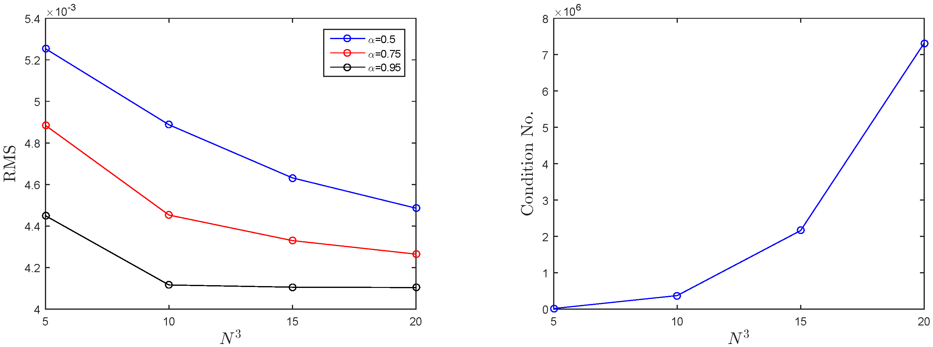
| Condition No. | 4.6506 × 10 | 7.2601 × 10 | 3.6585 × 10 | |||
© 2020 by the authors. Licensee MDPI, Basel, Switzerland. This article is an open access article distributed under the terms and conditions of the Creative Commons Attribution (CC BY) license (http://creativecommons.org/licenses/by/4.0/).
Share and Cite
Ahmad, I.; Ahmad, H.; Thounthong, P.; Chu, Y.-M.; Cesarano, C. Solution of Multi-Term Time-Fractional PDE Models Arising in Mathematical Biology and Physics by Local Meshless Method. Symmetry 2020, 12, 1195. https://doi.org/10.3390/sym12071195
Ahmad I, Ahmad H, Thounthong P, Chu Y-M, Cesarano C. Solution of Multi-Term Time-Fractional PDE Models Arising in Mathematical Biology and Physics by Local Meshless Method. Symmetry. 2020; 12(7):1195. https://doi.org/10.3390/sym12071195
Chicago/Turabian StyleAhmad, Imtiaz, Hijaz Ahmad, Phatiphat Thounthong, Yu-Ming Chu, and Clemente Cesarano. 2020. "Solution of Multi-Term Time-Fractional PDE Models Arising in Mathematical Biology and Physics by Local Meshless Method" Symmetry 12, no. 7: 1195. https://doi.org/10.3390/sym12071195