A Symmetric Banzhaf Cooperation Value for Games with a Proximity Relation among the Agents

Abstract

A cooperative game represents a situation in which a set of agents form coalitions in order to achieve a common good. To allocate the benefits of the result of this cooperation there exist several values such as the Shapley value or the Banzhaf value. Sometimes it is considered that not all communications between players are feasible and a graph is introduced to represent them. Myerson (1977) introduced a Shapley-type value for these situations. Another model for cooperative games is the Owen model, Owen (1977), in which players that have similar interests form a priori unions that bargain as a block in order to get a fair payoff. The model of cooperation introduced in this paper combines these two models following Casajus (2007). The situation consists of a communication graph where a two-step value is defined. In the first step a negotiation among the connected components is made and in the second one players inside each connected component bargain. This model can be extended to fuzzy contexts such as proximity relations that consider leveled closeness between agents as we proposed in 2016. There are two extensions of the Banzhaf value to the Owen model, because the natural way loses the group symmetry property. In this paper we construct an appropriate value to extend the symmetric option for situations with a proximity relation and provide it with an axiomatization. Then we apply this value to a political situation.

1. Introduction

Cooperative game theory describes the way to allocate the worth that result when a set of agents collaborate together in a coalition. A cooperative game with transfer utility is given as a characteristic function defining a worth for each coalition of agents. A value for a game is a function determining a payoff vector for each cooperative game. The most known value was introduced by Shapley [1]. From the political context another value was introduced by Banzhaf [2] and Dubey and Shapley [3], with similar properties to the Shapley value. The Shapley value can be used as an allocation of the worth of the great coalition but not the Banzhaf value. Both of them can be used as indices in the sense that they measure the power of the agents and then they allow to distribute all kind of goods taking into account the capacity of each player.

In the classic model there are not restrictions in cooperation. In real life, political, social or economic circumstances may impose certain constraints on coalition formation. This idea has led several authors to develop models of cooperative games with partial cooperation. One of the first approximations to partial cooperation is due to Aumann and Dreze [4]. A coalition structure is a partition of the set of players such that the cooperation is possible only if the players belong to the same element of the partition. They introduced the concept of value for games with coalition structure. In this case, the final coalitions are the elements of the partition, but inside each of them all coalitions are feasible. Myerson [5], in his seminal work Graphs and Cooperation in Games, presented a new class of games with partial cooperation structure. A communication structure is a graph on the set of players, where the links represent how the players can define feasible relations in the following sense: a coalition is feasible if and only if the subgraph generated by the vertices in that coalition is connected. This model is also an extension of the model of coalition structures, here the final coalition structure is the set of connected components. The Myerson value [5] determines a payoff vector for each game and each communication structure in the Shapley sense, moreover if the graph is complete this solution coincides with the Shapley value.

Owen [6] introduced a different model in partial cooperation. In this case the coalition structure is interpreted as a priori unions formed by the closeness among the players. Nevertheless these unions are not the final cooperation, they are a priori relationships determining the bargaining to get the great coalition. The Owen model defines a payoff vector in two steps, taking a game over the unions and later taking another game inside each union. Owen [6] also defined two values for games with a priori unions: the Owen value (considering the Shapley value in both steps) and the Banzhaf–Owen value (using the Banzhaf value in both steps). However, Alonso-Meijide and Fiestras-Janeiro [7] showed that the Banzhaf–Owen value loses one important property: the group symmetry, namely two unions with the same size and symmetric in the game obtain the same payoff. They considered a new value for games with a priori unions using the Banzhaf value among the unions and the Shapley value inside each union. Following the Myerson model, Casajus [8] raised a graph as a map of the a priori relations among the players in the Owen sense. This model, called cooperation structure, considers that the a priori unions are the connected components of the graph and the subgraph in each component explains the internal bilateral relationships among the players. The Myerson–Owen value is a two-step value like the Owen value that applies the Shapley value among the components and the Myerson value inside each component. It is defined an axiomatized in Fernández et al. [9]. Later Fernández et al. [10] introduced a Banzhaf value from the Owen version to the Casajus model. Now we define in this paper another Banzhaf solution for games in the Casajus model but from the Alonso-Meijide and Fiestras-Janeiro point of view, this in taking into account the symmetry in groups.

Aubin [11] considered games with fuzzy coalitions. In a fuzzy coalition the membership of the players is leveled. A critical issue arises when dealing with usual games and fuzzy coalitions: how to assign a worth to a fuzzy coalition from a usual game. Tsurumi et al. [12] used the Choquet integral [13] to extend a classic game to fuzzy coalitions and they introduced a value by a Choquet formula to define a Shapley value. Jiménez-Losada et al. [14] began to study games with partial cooperation from fuzzy coalition structures. They introduced the concept of fuzzy communication structure in a particular version and defined the Choquet by graphs partition of a fuzzy graph with the purpose of constructing values in this context; see [14,15,16]. Later the analyzed games with a proximity relation among the players, the Shapley value [9] and the Banzhaf value [10] (following the Owen version). Now we use the symmetric version introduced in this same paper to get another Banzhaf value for games with a proximity relation among the agents.

Section 2 sets preliminaries information about cooperative games, a priori unions and fuzzy sets. In Section 3 we recall the symmetric coalitional Banzhaf value and we extend it to the Casajus model. In Section 4 we extend again the cooperation value to proximity situations and we axiomatize it in Section 5. Section 6 compares the application of the new values in a political example with the other values for games with a proximity relation among the players. Section 7 is a short summary of conclusions. Finally, in Appendix A we include the proofs of the theorems.

2. Preliminaries

2.1. Cooperative Tu-Games

A cooperative game with transferable utility, game from now on, is a pair $(N,v)$ where N is a finite set, $v:2^N\to \mathbf{R}$ is a mapping with $v(\varnothing )=0$. The elements of $N=\{1,2,\dots ,n\}$ are called players. The mapping v is named characteristic function of the game. A subset $S\subseteq N$ is named coalition. The family of games will be denoted by $\mathcal{G}$. If $S\subseteq N,$ we denote by $(S,v_S)$ the restricted game, where $v_S$ is the restriction of v to $2^S.$ A payoff vector for a game $(N,v)$ is a vector $x\in {\mathbf{R}}^N$ so that $x_i$ is interpreted as the payment that the player $i\in N$ would receive for its cooperation. A value or solution for games is a mapping over $\mathcal{G}$ so that it assigns to each game $(N,v)$ a payoff vector $\phi (N,v)\in {\mathbf{R}}^N.$ Two of the most important values are the Shapley value $\varphi$ and the Banzhaf value $\beta ,$ defined by

$${\varphi }_i(N,v)=\sum _{S\subseteq N\backslash \left\{i\right\}}{\displaystyle \frac{\left|S\right|!(n-|S|-1)!}{n!}}[v(S\cup \left\{i\right\})-v\left(S\right)],$$

(1)

and

$${\displaystyle {\beta }_i(N,v)=\sum _{S\subseteq N\backslash \left\{i\right\}}{\displaystyle \frac{1}{2^{n-1}}}[v(S\cup \left\{i\right\})-v\left(S\right)].}$$

(2)

The Shapley value satisfies efficiency, i.e., ${\sum }_{i\in N}\varphi (N,v)=v\left(N\right)$. It is also linear, i.e., if $(N,v_1)$, $(N,v_2)\in \mathcal{G}$ and $\alpha ,\beta \in \mathbf{R}$ then $\varphi (N,\alpha v_1+\beta v_2)=\alpha \varphi (N,v_1)+\beta \varphi (N,v_2)$. A null player $i\in N$ for a game $(N,v)$ satisfies $v(S\cup \{i\left\}\right)=v\left(S\right),\forall S\subseteq N\backslash \left\{i\right\}.$ The Shapley value satisfies the null player axiom i.e., if i is a null player for $(N,v)$ then ${\varphi }_i(N,v)=0$. It is said that $i,j\in N$ are substitutable players in a game $(N,v)$ if $v(S\cup \{i\left\}\right)=v(S\cup \{j\left\}\right),\forall S\subseteq N\backslash \{i,j\}$. The equal treatment axiom says that if $i,j\in N$ are substitutable players in $(N,v)$ then ${\varphi }_i(N,v)={\varphi }_j(N,v)$. It is known that the Shapley value is the only allocation rule over $\mathcal{G}$ satisfying efficiency, linearity, null player and equal treatment. Moreover these axioms are not redundant. The Banzhaf value satisfies pairwise merging, linearity, null player and equal treatment. Pairwise merging uses the amalgamated game of $(N,v)$ for $i,j\in N.$ It is another game $(N^{ij},v^{ij})$ where $N^{ij}=N\backslash \{i,j\}\cup \left\{p\right\}$ and for every $S\subseteq N^{ij}$,

$$v^{ij}\left(S\right)=\left\{\begin{array}{cc}v(S\backslash \{p\}\cup \{i,j\left\}\right),\hfill & if p\in S\hfill \\ v\left(S\right),\hfill & if p\notin S.\hfill \end{array}\right.$$

The Banzhaf value $\beta$ satisfies the pairwise merging axiom, i.e., for each $(N,v)\in \mathcal{G}$ and each pair of players $i,j\in N$ we have ${\beta }_p(N^{ij},v^{ij})={\beta }_i(N,v)+{\beta }_j(N,v).$

2.2. Communication Structures

Myerson [5] thought that sometimes not all communications between players are feasible. He introduced a graph as a representation of this situation. Let N be a finite set of players and $L^N=\{\{i,j\}\in N\times N:i\ne j\}$ the set of unordered pairs of different elements in N. We will use $ij=\{i,j\}$ by abuse of notation. A communication structure L for N is a graph with set of vertices N and set of links $L\subseteq L^N$. A game with communication structure is a triple $(N,v,L)$ where $(N,v)\in \mathcal{G}$ and L is a communication structure for N. The family of games with communication structure will be denoted by $\mathcal{GC}.$ A game $(N,v)\in \mathcal{G}$ can be identified with the game with communication structure $(N,v,L^N)$. Let $(N,v,L)$ be a game with communication structure. A coalition $S\subseteq N$ is called connected in L if for each pair of different players $i,j\in S$ there exists a sequence $i_0,\dots ,i_k\in S$ with $i_{p-1}{i}_p\in L$ for all $p=1,\dots ,k$, $i_0=i$ and $i_k=j$. Individual coalitions are considered connected. The communication structure L for N is called connected if N is connected in L (this concept coincides with the notion of connected graph). The maximal connected coalitions (by inclusion) are named the connected components (the connected components form always a partition of N) of L and will be denoted by $N/L$. If $S\subseteq N$ then the restricted communication structure for S is $L_S=\{ij\in L:i,j\in S\}.$ We write $S/L=S/L_S$, i.e., the connected components of $L_S$ as communication structures for S. Myerson introduced the graph game $\left(N,v/L\right)$ that includes the information of the communication structure,

$$v/L\left(S\right)=\sum _{T\in S/L}v\left(T\right)\forall S\subseteq N.$$

(3)

The Shapley value was extended for games with communication structure in [5]. The Myerson value is a function defined as

$$\mu (N,v,L)=\varphi \left(N,v/L\right).$$

(4)

Myerson proved that his value is the only one satisfying the following axioms:

(M1)

Component efficiency. For each $S\in N/L,{\sum }_{i\in S}{\mu }_i(N,v,L)=v\left(S\right).$

(M2)

Fairness. If $ij\in L$ then ${\mu }_i(N,v,L)-{\mu }_i(N,v,L\backslash \left\{ij\right\})={\mu }_j(N,v,L)-{\mu }_j(N,v,L\backslash \left\{ij\right\})$.

The Myerson value is also component decomposable, i.e., if $S\in N/L$ then ${\mu }_i(N,v,L)={\mu }_i(S,v,L_S)$ for all $i\in S$.

2.3. A Priori Unions

The Owen’s approach supposes that the players are organized in a priori unions that have common interests in the game. However, these unions are not considered as a final structure but as a starting point for further negotiations. So each union negotiates as a whole with the other unions to achieve a fair payoff. A game with a priori unions is a triple $\left(N,v,\mathcal{P}\right)$ where $(N,v)$ is a game and $\mathcal{P}=\left\{N_1,\dots ,N_m\right\}$ is a partition of N. We will denote the set of games with a priori unions by $\mathcal{GU}$. A value for games with a priori unions is a mapping f that assigns a payoff vector $f(N,v,\mathcal{P})\in {\mathbf{R}}^N$ to each $(N,v,\mathcal{P})\in \mathcal{GU}.$ Owen [6] proposed a method to obtain values for games with a priori unions, which is defined in two steps. First we need some definitions. Let $\left(N,v,\mathcal{P}\right)\in \mathcal{GU}$ with $\mathcal{P}=\left\{N_1,\dots ,N_m\right\}$. The quotient game is a game $\left(M,v^{\mathcal{P}}\right)$ with set of players $M=\{1,\dots ,m\}$ defined by

$$v^{\mathcal{P}}\left(Q\right)=v\left(\bigcup _{q\in Q}{N}_q\right),\forall Q\subseteq M.$$

(5)

Let $\left(N,v,\mathcal{P}\right)\in \mathcal{GU}$, $\mathcal{P}=\left\{N_1,\dots ,N_m\right\}$ and $k\in M$. For each $S\subset N_k$ the partition ${\mathcal{P}}_S$ of $\left(N\backslash N_k\right)\cup S$ consists of replacing $N_k$ with S, i.e.,

$${\mathcal{P}}_S=\left\{N_1,\dots ,\stackrel{k)}{S},\dots ,N_m\right\}.$$

(6)

Let $f^1$ be a classic value for games. The first step consists of a negotiation among unions that is focused on $S.$ The result of the quotient game generates a new game in $N_k.$ We define the game $\left(N_k,v_k\right)$ by

$$v_k\left(S\right)=f_k^1\left(M,v^{{\mathcal{P}}_S}\right),\forall S\subseteq N_k.$$

(7)

In the second step the game in every group is solved using another classic value $f^2$. So, for each player $i\in N,$ if $k\left(i\right)$ is such that $i\in N_{k\left(i\right)}$ then the new value f is defined by

$$f_i\left(N,v,\mathcal{P}\right)=f_i^2\left(N_{k\left(i\right)},v_{k\left(i\right)}\right).$$

(8)

The first values for games with a priori unions were introduced in [6], one of them (the Owen value) applies the Shapley value in both steps of the negotiation and the another one applies the Banzhaf value in both. Alonso-Meijide and Fiestra-Janeiro [7] observed that the Banzhaf value of Owen for a priori unions loses an important property for a value, it does not satisfy the group symmetry. A value f for games with a priori unions satisfies group symmetry if for all pair of groups $N_p,N_q\in \mathcal{P}$ with $v(N_p\cup S)=v(N_q\cup S)$ if $S\subseteq N\backslash (N_p\cup N_q)$. They introduced a new Banzhaf value for these situations, the symmetric version. We will extend here the symmetric coalitional Banzhaf value (that applies the Shapley value among the unions and the Banzhaf value inside each union).

In the Owen model players are organized in a priori unions but there is no information about the internal structure of these unions. Casajus [8] proposed a modification of the Owen model in the Myerson sense. We call this model games with cooperation structure. A cooperation structure is a graph where the connected components represent the a priori unions, but the links give us additional information about how they are formed. A game with cooperation structure is a triple $(N,v,L)$ with $(N,v)\in \mathcal{G}$ and $L\subseteq L^N.$ The family of games with cooperation structure is denoted by $\mathcal{GCO}.$ By definition $\mathcal{GC}=\mathcal{GCO};$ nevertheless the interpretation is completely different. Moreover we have $\mathcal{GU}\subset \mathcal{GCO},$ because an a priori union structure can be identified with a cooperation structure with complete components. A value for games with cooperation structure is a mapping f that assigns a payoff vector $f(N,v,L)\in {\mathbf{R}}^N$ to each $(N,v,L)\in \mathcal{GCO}$. Casajus [8] proposed to follow the model of Owen to get a value for games with cooperation structure. Given $(N,v,L)\in \mathcal{GCO},$ we consider the partition of N by its connected components $N/L$. Therefore $N/L$ is a set of a priori unions for the players in N but the links in L tell us how these unions are formed. We use the same quotient game (5) with the partition $N/L=\left\{N_1,\dots ,N_m\right\}$ and also the same first game $v_k$ (7) with a particular chosen value $f^1$. In the second step we consider a communication value $f^2$ to allocate the profit inside each component. For each $i\in N$ let $k\left(i\right)$ the index such that $i\in N_{k\left(i\right)}$. The new value f is defined by

$$f_i^2\left(N_{k\left(i\right)},v_{k\left(i\right)},L_{N_{k\left(i\right)}}\right).$$

Casajus defined a value using the Shapley value in the first step and the Myerson value in the second step and gave an axiomatization. Another one was given in [9]. Fernández et al. [10] defined an extension of the non-symmetric version of the Banzhaf value to the Casajus model. In this paper we consider a cooperation value consisting of applying the Banzhaf value in the first step and the Myerson value in the second step in order to get a symmetric version.

2.4. Fuzzy Sets and Proximity Relations

In classical set theory, the membership of elements in a set is assessed in binary terms according to a bivalent condition, an element either belongs or does not belong to the set. By contrast, fuzzy set theory permits the gradual assessment of the membership of elements in a set. In this subsection we are going to recall some concepts related to fuzzy sets and the Choquet integral that will be useful subsequently. We will use $\vee ,\wedge$ to denote the maximum and the minimum respectively. A fuzzy set of a finite set K is a mapping $\tau :K\to [0,1]$. Obviously, any classic set $A\subseteq K$ is identified with a fuzzy set $e^A$ where $e^A\left(i\right)=1$ if $i\in A$ and $e^A\left(i\right)=0$ otherwise. The support of $\tau$ is the set $supp\left(\tau \right)=\{i\in K:\tau (i)\ne 0\}$. The image of $\tau$ is the ordered set of the non-null images of the function, $im\left(\tau \right)=\{\lambda \in (0,1]:\exists i\in K,\tau (i)=\lambda \}.$ The family of fuzzy sets over a finite set K will be denoted by ${[0,1]}^K.$ Sometimes, for convenience, the image of a fuzzy set is expressed by $im\left(\tau \right)=\left\{{\lambda }_1<\cdots <{\lambda }_p\right\}.$ Two fuzzy sets $\tau ,{\tau }^{\prime }$ are comonotone if for all $i,j\in K$ it holds $(\tau \left(i\right)-\tau \left(j\right))({\tau }^{\prime }\left(i\right)-{\tau }^{\prime }\left(j\right))\ge 0.$ Comonotony is an equivalence relation in ${[0,1]}^K.$ A fundamental tool for the analysis of fuzzy sets are the so-called cuts. For each $t\in (0,1]$ the t-cut of the fuzzy set $\tau$ is

$${\left[\tau \right]}_t=\{i\in K:\tau \left(i\right)\ge t\}.$$

(9)

The Choquet integral is an aggregation operator defined in [13]. Given $f:2^K\to \mathbf{R}$ and $\tau$ a fuzzy set over K, the (signed) Choquet integral of $\tau$ with respect to f is defined as

$$\int \tau df=\sum _{k=1}^p\left({\lambda }_k-{\lambda }_{k-1}\right)f\left({\left[\tau \right]}_{{\lambda }_k}\right),$$

(10)

where $im\left(\tau \right)=\left\{{\lambda }_1<\cdots <{\lambda }_p\right\}$ and ${\lambda }_0=0$.

The following properties of the Choquet integral are known:

(C1)

${\displaystyle \int e^{S}df=f\left(S\right)}$, for all $S\subseteq K.$

(C2)

${\displaystyle \int t\tau df=t\int \tau df}$, for all $t\in \left[0,1\right].$

(C3)

${\displaystyle \int \tau d\left(a_1{f}_1+a_2{f}_2\right)=a_1\int \tau d{f}_1+a_2\int \tau d{f}_2,}$ when $a_1,a_2\in \mathbf{R}.$

(C4)

${\displaystyle \int \left(\tau +{\tau }^{\prime }\right)df=\int \tau df+\int {\tau }^{\prime }df,}$ when $\tau +{\tau }^{\prime }\le e^K$ and $\tau ,{\tau }^{\prime }$ are comonotone.

(C5)

${\displaystyle \int \tau df=A\underset{i\in N}{\bigvee }\tau \left(i\right)}$ if $f\left({\left[\tau \right]}_t\right)=A,$ for all $t\in im\left(\tau \right)$.

In this paper we focus on a particular case of fuzzy relations. A bilateral fuzzy relation, see [17], over K is a function $\phi :K\times K\to [0,1]$ satisfying $\phi (i,j)\le \phi (i,i)\wedge \phi (j,j).$ A proximity relation over K, is a fuzzy relation $\phi$ satisfying: (Reflexivity) $\phi (i,i)=1$ for all $i\in K$ and (Symmetry) $\phi (i,j)=\phi (j,i)$ for all $i,j\in K$.

3. the Banzhaf–Myerson Value

Fernandez et al. [10] defined a Banzhaz value following [6] for the Casajus model [8]. However, this value fails in an important condition for a value: the symmetry for groups as we can see in [7] (a priori unions are particular cases of the Casajus model). Now we propose a new Banzhaf value with a group symmetry property (here in this context it is denominated substitutable components). The cooperation value that we present applies the Banzhaf value among the unions and the Myerson value within the unions.

Definition 1.

The Banzhaf–Myerson value δ is an allocation rule defined over the class of games with cooperation structure by

$${\delta }_i(N,v,L)={\mu }_i\left(N_{k\left(i\right)},v_{k\left(i\right)},L_{N_{k\left(i\right)}}\right),$$

where $k\left(i\right)$ is such that $i\in N_{k\left(i\right)}$ and $v_{k\left(i\right)}\left(S\right)={\beta }_{k\left(i\right)}\left(M,v^{{(N/L)}_S}\right)$ for each $S\subseteq N_{k\left(i\right)}.$

If we look at the Casajus model, in this case, $f^1=\beta$ and $f^2=\mu$.

The Banzhaf–Myerson value is a generalization of the symmetric coalitional Banzhaf value $\phi$ defined in [7], but taking into account the inner structure of the a priori unions, in this case $N/L.$ The Banzhaf–Myerson solution satisfies the following coincidences.

(a)

If $(N,v,L)\in \mathcal{GCO}$ satisfies that L is connected then $\delta (N,v,L)=\mu (N,v,L)$.

(b)

If $(N,v,L)\in \mathcal{GCO}$ satisfies that $L_S=L^S$ for all $S\in N/L$ then we identify $(N,v,L)$ with $\left(N,v,N/L\right)\in \mathcal{GU}$ and $\delta (N,v,L)=\phi \left(N,v,N/L\right),$ where $\phi$ is the symmetric coalitional Banzhaf value.

(c)

If $(N,v,L)\in \mathcal{GCO}$ with $L=L^N$ then $\delta (N,v,L)=\varphi (N,v)$.

With the purpose of obtaining an axiomatization we introduce some axioms. The first four axioms also appear in the axiomatization of the Myerson–Owen value in [9]. We will also prove that this value is a coalitional value of Banzhaf.

Definition 2.

A coalitional value of Banzhaf f over $\mathcal{GCO}$ is a cooperation value that satisfies

$$f(N,v,\varnothing )=\beta (N,v),$$

where ∅ denotes the empty graph, i.e., the graph without links.

In spite of the strategic position of each agent, a component cannot obtain profits if all its players in are null. We say that a coalition $S\subseteq N$ is a null coalition in a game $(N,v)\in \mathcal{G}$ if each player $i\in S$ is a null player in the game, i.e., $v(T\cup \{i\left\}\right)=v\left(T\right),\forall T\subseteq N\backslash \left\{i\right\}$.

Null component. Let $(N,v,L)\in \mathcal{GCO}$ and $S\in N/L$ a null coalition, then $f_i(N,v,L)=0$ for all $i\in S$.

Two coalitions $S,T\subseteq N$ with $S\cap T=\varnothing$ are substitutable in a game $(N,v)$ if $v(R\cup S)=v(R\cup T)$ for all $R\subseteq N\backslash (S\cup T)$. We consider that substituible components must get the same total outcome. The following axiom is an extension of the group symmetry axiom for games with a priori unions. This is the main difference between this Banzhaf value and that introduced in [10].

Substitutable components. Let $(N,v,L)\in \mathcal{GCO}$. If $S,T\in N/L$ are substitutable components in $(N,v)$ then

$$\sum _{i\in S}{f}_i(N,v,L)=\sum _{j\in T}{f}_j(N,v,L).$$

The asymmetry of the structure of each component modifies the equal treatment property within the unions used in the axiomatization of the Owen value. In our case the Myerson fairness is not enough to fix this asymmetry because the deletion of a link can cause a change in the number of components. So, we use the modified fairness proposed in [8]. This axiom says that the difference of payoffs when we break a link, placing the players disconnected by this fact out of the game, is the same for both of the players in the link. Let $(N,v,L)\in \mathcal{GCO}$ and $ij\in L$. If $S\in N/L$ with $i,j\in S$ and $S_i\in N/(L\backslash \left\{ij\right\})$ with $i\in S_i$ (in the same way $S_j$) then $N_{ij}^i=(N\backslash S)\cup S_i$ (in the same way $N_{ij}^j$).

Modified fairness. Let $(N,v,L)\in \mathcal{GCO}$ and $ij\in L$, it holds

$$\begin{array}{ccc}\hfill f_i(N,v,L)-f_i\left(N_{ij}^i,v,L_{N_{ij}^i}\backslash \left\{ij\right\}\right)& =& f_j(N,v,L)-f_j\left(N_{ij}^j,v,L_{N_{ij}^j}\backslash \left\{ij\right\}\right).\hfill \end{array}$$

We also add the typical axioms of linearity and efficiency for a particular case.

Linearity. Let $(N,v_1,L),(N,v_2,L)\in \mathcal{GCO},$$\alpha ,\beta \in \mathbf{R}.$ Then

$$f(N,\alpha v_1+\beta v_2,L)=\alpha f(N,v_1,L)+\beta f(N,v_2,L).$$

Connected efficiency. A cooperation value f satisfies connected efficiency if

$$\sum _{i\in N}{f}_i(N,v,L)=v\left(N\right),$$

for every L that is connected.

The following axiom is a property for the situation in which we connect two components. First we define this modification of a graph.

Definition 3.

Let $(N,v,L)\in \mathcal{GCO}$, $N_r,N_s\in N/L$ and $i_k\in N_k,k=r,s$. If we add the edge $\left\{i_r{i}_s\right\}$ we define the graph $L_{N_r{N}_s}=L\cup \left\{i_r{i}_s\right\}.$

Component merging. A cooperation value f satisfies component merging if for every $r,s\in M,$

$$\sum _{k\in N_r\cup N_s}{f}_k(N,v,L)=\sum _{k\in N_r\cup N_s}{f}_k\left(N,v,L_{N_r{N}_s}\right).$$

Theorem 1.

The Banzhaf–Myerson value δ is a coalitional value of Banzhaf that satisfies connected efficiency, component merging, null component, substitutable components, modified fairness and linearity.

Theorem 2.

The Banzhaf–Myerson value δ is the only cooperation value that satisfies connected efficiency, component merging, null component, substitutable components, modified fairness and linearity.

If we compare the axiomatizations of the Myerson–Owen value in [9] and the Banzhaf–Myerson value, the latter differs from the first in the fact that connected efficiency and component merging replace efficiency. This seems a logical consequence from the axiomatizations of the Shapley value and the Banzhaf value presented before. They have in common linearity, symmetry and null player. Nevertheless, the Shapley value is efficient, whereas the Banzhaf value satisfies pairwise merging.

4. Value for Games with a Proximity Relation

The goal of this paper is to define and axiomatize a value for games with a proximity relation among the players.

Definition 4.

A game with a proximity relation is a triple $(N,v,\rho )$ where $(N,v)\in \mathcal{G}$ and ρ is a proximity relation over N. The family games with a proximity relation is denoted as $\mathcal{GP}$.

A proximity relation can represent the level of coincidence between players, for instance in interests, ideas, etc. We write $\rho (i,j)=\rho \left(ij\right)$ from now on.

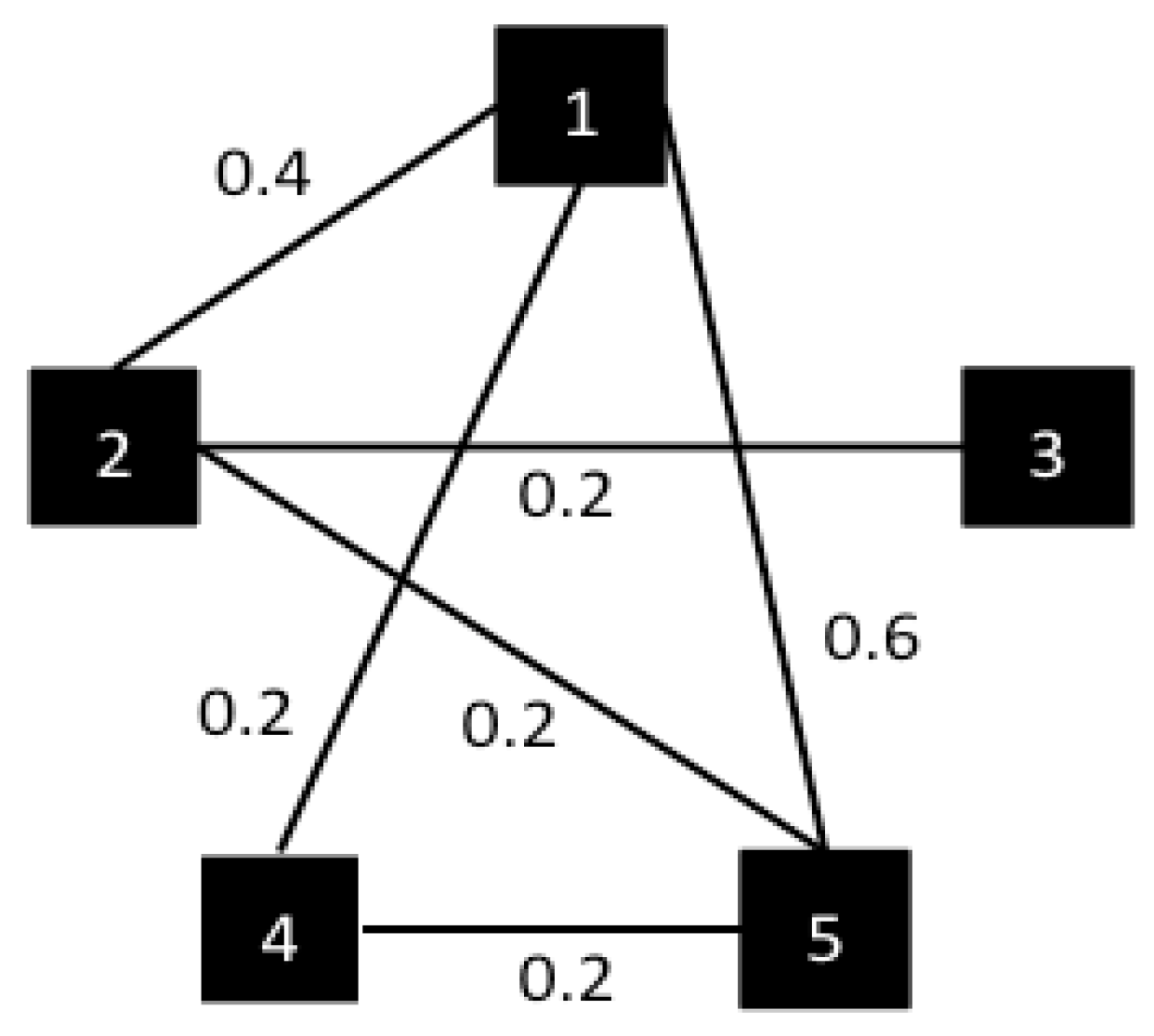
For example, consider $N=\{1,2,3,4,5\}$ a set of five agents. They cooperate to obtain the maximum profit making use of a land. The owners of the land are the agents 2 and 3, the rest of them are workers. However, there exist also particular relationships among the agents which can influence in the decision: players 1 and 2 are relatives, players 1, 2 and 5 are friends since their youth, and finally players 1 and 5 are supporters of the same football team. The characteristic function is the profit (in millions of euros) obtained depending on who owner cooperate (which part of the land is used),

$$v\left(S\right)=\left\{\begin{array}{cc}48\left(\right|S|-2),\hfill & \mathrm{if}2,3\in S\hfill \\ 10\left(\right|S|-1),\hfill & \mathrm{if}2\in S\mathrm{but}3\notin S\hfill \\ v\left(S\right)=16\left(\right|S|-1),\hfill & \mathrm{if}3\in S\mathrm{but}2\notin S\hfill \\ 0,\hfill & \mathrm{otherwise}.\hfill \end{array}\right.$$

Suppose all the kinds of relations with the same importance, we propose next proximity relation $\rho$ to represent them: $\rho (i,i)=1$ for all i, $\rho (1,5)=0.6,\rho (1,2)=0.4,\rho (1,4)=\rho (2,3)=\rho (2,5)=\rho (4,5)=0.2$ and $\rho (i,j)=0$ otherwise. Figure 1 shows the relations as a fuzzy graph.

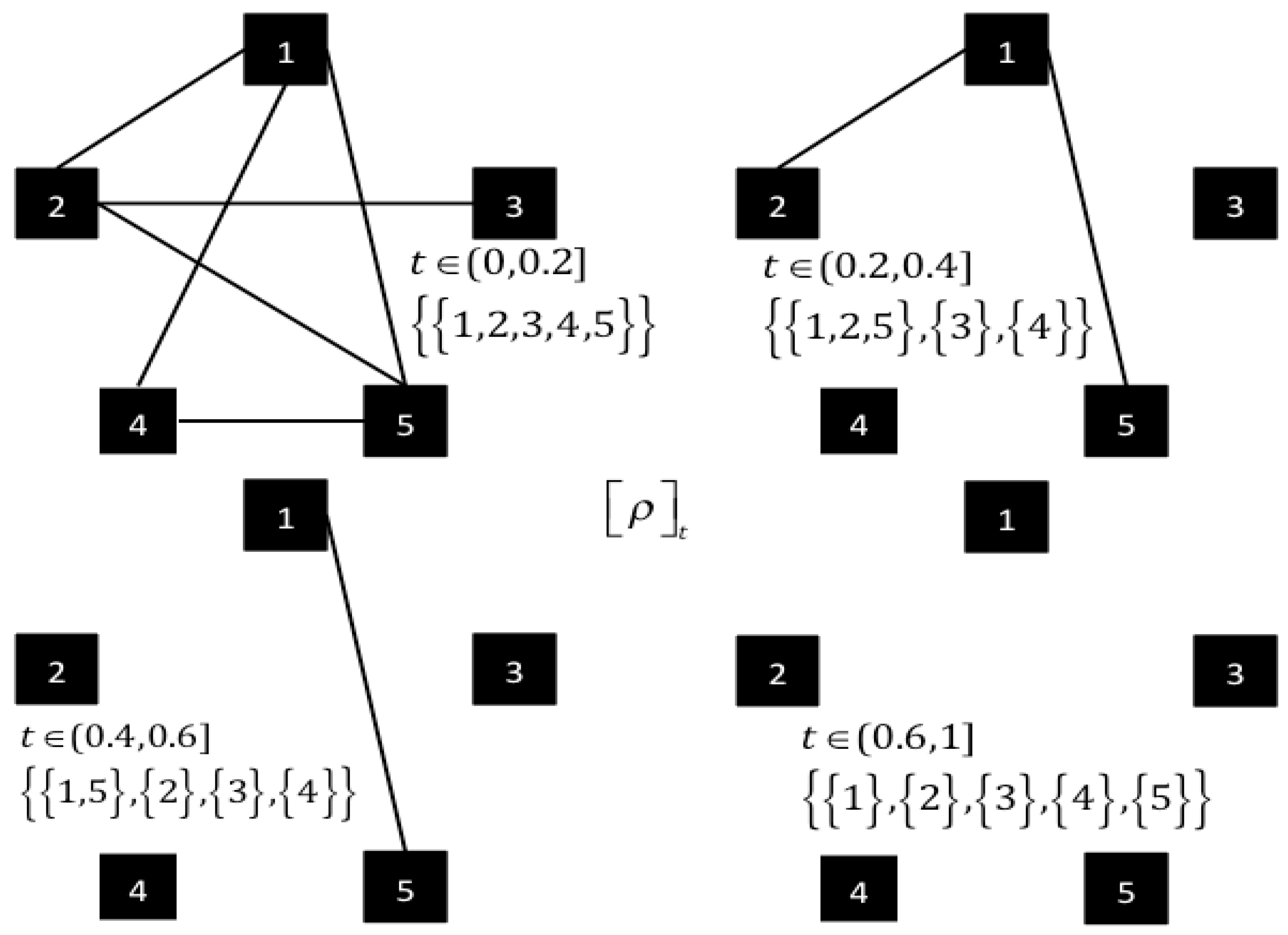
Now we extend the Owen model in a fuzzy way. A proximity relation can be seen as a cooperation structure by levels of the players. Let $(N,v,\rho )\in \mathcal{GP}$. For each $t\in (0,1]$ we have a cooperation structure. We obtain then a partition of the proximity relation in cooperation structures as we can see in the following figure. Casajus considers the different connected components as unions with internal structure. We recall the concept of group that appears in [9]. This is an extension of the unions in an a priori union structure.

Next defitions were introduced in [9]. Let $\rho$ be a proximity relation over N. A coalition $S\subseteq N$ is a t-group for $\rho$ with $t\in (0,1]$ if $S\in N/{\left[\rho \right]}_t$. The family of groups of $\rho$ is the set

$$N/\rho =\bigcup _{t\in (0,1]}N/{\left[\rho \right]}_t.$$

(11)

Let $\rho$ be a proximity relation over $N.$ Coalitions $S_1,\dots ,S_r\subseteq N$ are leveled groups if there is a number $t\in (0,1]$ such that $S_1,\dots ,S_r$ are t-groups. For each set of leveled groups $S_1,\dots ,S_r,(r\ge 1)$ we denote

$$t_{S_1\dots S_r}=\bigwedge \left\{t\in (0,1],S_1,\dots ,S_r\in N/{\left[\rho \right]}_t\right\}$$

(12)

$$t^{S_1\dots S_r}=\bigvee \left\{t\in (0,1],S_1,\dots ,S_r\in N/{\left[\rho \right]}_t\right\}$$

(13)

Fernández et al. [9] also introduced two ways to rescale a proximity relation and the relation between these scalings and the Choquet integral. Let $\rho$ be a proximity relation over N. If $a,b\in [0,1]$ with $a<b$ then ${\rho }_a^b$ is the interval scaling of $\rho$, a new proximity relation over N defined as

$${\rho }_a^b\left(ij\right)=\left\{\begin{array}{cc}1,\hfill & if \rho \left(ij\right)\ge b\hfill \\ {\displaystyle \frac{\rho \left(ij\right)-a}{b-a}},\hfill & if \rho \left(ij\right)\in (a,b)\hfill \\ 0,\hfill & if \rho \left(ij\right)\le a.\hfill \end{array}\right.$$

(14)

Let $a,b\in [0,1]$ be numbers with $a<b$ and $a\ne 0$ or $b\ne 1$. The dual interval scaling of $\rho$ is a new proximity relation over N given by

$${\overline{\rho }}_a^b\left(ij\right)=\left\{\begin{array}{cc}{\displaystyle \frac{\rho \left(ij\right)+a-b}{1+a-b}},\hfill & if \rho \left(ij\right)\ge b\hfill \\ {\displaystyle \frac{a}{1+a-b}},\hfill & if \rho \left(ij\right)\in (a,b)\hfill \\ {\displaystyle \frac{\rho \left(ij\right)}{1+a-b}},\hfill & if \rho \left(ij\right)\le a.\hfill \end{array}\right.$$

(15)

To aggregate the information of the proximity relation we use the Choquet integral.

Lemma 1

([9]). Let ρ be a proximity relation over N. For every pair of numbers $a,b\in [0,1]$ with $a<b$ and for every set function f over $L^N$ it holds

$$\int \rho df=(b-a)\int {\rho }_a^{b}df+(1+a-b)\int {\overline{\rho }}_a^{b}df.$$

We define the set function

$${\delta }_i(N,v)\left(L\right)={\delta }_i(N,v,L),\forall L\subseteq L^N,\forall i\in N.$$

We introduce the prox-Banzhaf–Myerson value for games with cooperation structure. It is the Choquet integral of the proximity relation with respect to the Banzhaf–Myerson set function.

Definition 5.

Let $(N,v,\rho )$ be a simple game with a proximity relation. The prox-Banzhaf–Myerson value is defined by

$$Z_i(N,v,\rho )=\int \rho d{\delta }_i(N,v).$$

Suppose the game of our example in Figure 1. Depending on the assumed information we obtain the following solutions. If we only consider the game, we have that the Shapley value is $\varphi (N,v)=(20.333,37,46,20.333,20.333).$ If we consider only the communication structure L in Figure 1 without the numbers on the links we apply the Banzhaf–Myerson value of the game (which coincides with the Myerson value because the graph is connected), $\delta (N,v,L)=(20.4,50.9,36.733,15.566,20.4).$ Finally we calculate the prox-Banzhaf–Myerson value. We have to consider the different graphs in Figure 2 to determine the Choquet integral. So, for each player $i\in N=\{1,2,3,4,5\},$

$$\begin{array}{ccc}\hfill Z(N,v,\rho )& =& (0.2-0)\delta (N,v)\left({\left[\rho \right]}_{0.2}\right)+(0.4-0.2)\delta (N,v)\left({\left[\rho \right]}_{0.4}\right)+(0.6-0.4)\delta (N,v)\left({\left[\rho \right]}_{0.6}\right)\hfill \\ & & +(1-0.6)\delta (N,v)\left({\left[\rho \right]}_1\right)\hfill \\ & =& 0.2\left(20.4,50.9,36.733,15.566,20.4\right)+0.2\left(25.5,28,51.5,18.5,15\right)\hfill \\ & & +0.3\left(18.5,31.5,40.5,18.5,18.5\right)+0.3\left(18.5,31.5,40.5,18.5,18.5\right)\hfill \\ & =& (20.28,34.68,41.9467,17.9133,18.18).\hfill \end{array}$$

5. Axiomatization of the Value

We say that $\rho$ is connected if $\exists t\in (0,1]$ such that ${\left[\rho \right]}_t$ is connected. In that case

$$t^{\rho }=\bigvee \left\{t\in [0,1]:{\left[\rho \right]}_t\mathrm{connected}\right\}$$

(16)

is called connection level of $\rho .$

We are going to see some axioms for Z that are a fuzzy extension of the axioms already presented for $\delta .$

Fuzzy connected efficiency. A proximity value F satisfies fuzzy connected efficiency if $\forall (N,v,\rho )\in \mathcal{GP}$ with $\rho$ connected it holds

$$\sum _{i\in N}{F}_i(N,v,\rho )-(1-t^{\rho })F_i\left(N,v,{\rho }_{t^{\rho }}^1\right)=t^{\rho }v\left(N\right).$$

If $\left|im\right(\rho \left)\right|=1$ and $\rho$ is connected then $t^{\rho }=1$ and the axiom reduces to connected efficiency.

Let $(N,v,\rho )\in \mathcal{GP}.$ If $t\in [0,1-\rho (ij\left)\right],$ with $i,j\in N$ we can introduce the proximity relation ${\rho }_{+ij}^t,$ where

$${\rho }_{+ij}^t\left(kl\right)=\left\{\begin{array}{cc}\rho \left(kl\right),\hfill & \mathrm{if}kl\ne ij\hfill \\ \rho \left(ij\right)+t,\hfill & \mathrm{if}kl=ij.\hfill \end{array}\right.$$

Then the fuzzy extension of component merging is constructed using this proximity relation.

Group merging. A proximity value F satisfies group merging if for every pair of leveled groups $S,T$ and each pair $i\in S,j\in T$ it holds

$$\begin{array}{ccc}\hfill \sum _{k\in S\cup T}{F}_k(N,v,\rho )& -& \left(1+t_{ST}-t^{ST}\right)F_k\left(N,v,{\overline{\rho }}_{t_{ST}}^{t^{ST}}\right)\hfill \\ & =& \sum _{k\in S\cup T}{F}_k\left(N,v,{\rho }_{+ij}^{t^{ST}-\rho \left(ij\right)}\right)-\left(1+t_{ST}-t^{ST}\right)F_k\left(N,v,{\left(\overline{{\rho }_{+ij}^{t^{ST}-\rho \left(ij\right)}}\right)}_{t_{ST}}^{t^{ST}}\right).\hfill \end{array}$$

Notice that $\rho \left(ij\right)\le t_{ST}$ by (12).

• If $\left|im\right(\rho \left)\right|=1$ group merging reduces to component merging.
• If a coalition is null then its players do not get profits when it is considered as a union or a partition of unions, therefore we can take as negligible cases these levels and later rescale.

Null group. Let $(N,v,\rho )\in \mathcal{GP}$ and $S\in N/\rho$ a group which is null for the game $(N,v)$ then

$$F_i(N,v,\rho )=t_S{F}_i\left(N,v,{\rho }_0^{t_S}\right),\forall i\in S.$$

Particularly if we consider a crisp proximity relation $\rho$ (a cooperation structure) the axiom says: “if S is a component for $\rho$ which is a null coalition for the game $(N,v)$ then $F_i(N,v,\rho )=0$ for all $i\in S$”, i.e., it coincides with the null component axiom.

We take two substitutable coalitions. We can suppose that while both coalitions are groups the total payoff for each group is the same, that is

$$\sum _{i\in S}{F}_i\left(N,v,{\rho }_{t_{ST}}^{t^{ST}}\right)=\sum _{j\in T}{F}_j\left(N,v,{\rho }_{t_{ST}}^{t^{ST}}\right).$$

(17)

However, we can get a similar condition using the next axiom, the part of the payoffs for each group which is not obtained in the common interval must be the same.

Substitutable leveled groups Let $(N,v,\rho )\in \mathcal{GP}$. If $S,T\in N/\rho$ are leveled groups and they are substitutable in $(N,v)$ then

$$\sum _{i\in S}{F}_i(N,v,\rho )-\left(1+t_{ST}-t^{ST}\right)F_i\left(N,v,{\overline{\rho }}_{t_{ST}}^{t^{ST}}\right)=\sum _{j\in T}{F}_j(N,v,\rho )-\left(1+t_{ST}-t^{ST}\right)F_j\left(N,v,{\overline{\rho }}_{t_{ST}}^{t^{ST}}\right).$$

If we consider a proximity relation $\rho$ which is crisp the axiom says: if $S,T$ are substitutable components of $\rho$ for a game $(N,v)$ then ${\sum }_{i\in S}{F}_i(N,v,\rho )={\sum }_{j\in T}{F}_j(N,v,\rho ),$ i.e., it coincides with the substitutable components axiom. Observe that, by Lemma 1, our value verifies the substitutable leveled groups axiom if and only if we get (17).

The modified fairness axiom [8] can be extended to proximity relations. Now, we do not consider the deletion of links but the reduction of level. The axiom only affects to the levels in the interval between the reduced level and the original one. Let $\rho$ be a proximity relation over a set of players N with $im\left(\rho \right)=\{{\lambda }_1<\cdots <{\lambda }_m\}$ and ${\lambda }_0=0.$ Consider $i,j\in N$ two different players with $\rho \left(ij\right)={\lambda }_k>0.$ The number ${\rho }^{*}\left(ij\right)={\lambda }_{k-1}$ satisfies that for all $t\in \left({\rho }^{*}\left(ij\right),\rho \left(ij\right)\right]$ the set $N_{ij}^i$ (or $N_{ij}^j$) in the cooperation structure ${\left[\rho \right]}_t$ is the same. We denote also as $N_{ij}^i$ (or $N_{ij}^j$) this common set for $\rho .$ Now the modified fuzzy fairness says that the modified fairness is true if we reduce by t the closeness of link $ij$ for the outcomes in $\left(\rho \right(ij)-t,\rho (ij\left)\right]$, adding the outcomes obtained out of the interval.

Modified fuzzy fairness Let $(N,v,\rho )\in \mathcal{GP}$ and $i,j\in N$ with $\rho \left(ij\right)>0$. For each $t\in \left(0,\rho \left(ij\right)-{\rho }^{*}\left(ij\right)\right]$ it holds

$$\begin{array}{ccc}\hfill F_i(N,v,\rho )& -& F_j(N,v,\rho )=(1-t)\left[F_i\left(N,v,{\overline{\rho }}_{\rho \left(ij\right)-t}^{\rho \left(ij\right)}\right)-F_j\left(N,v,{\overline{\rho }}_{\rho \left(ij\right)-t}^{\rho \left(ij\right)}\right)\right]\hfill \\ & +& t\left[F_i\left(N_{ij}^i,v,{\left({\left({\rho }_{\rho \left(ij\right)-t}^{\rho \left(ij\right)}\right)}_{-ij}^1\right)}_{N_{ij}^i}\right)-F_j\left(N_{ij}^j,v,{\left({\left({\rho }_{\rho \left(ij\right)-t}^{\rho \left(ij\right)}\right)}_{-ij}^1\right)}_{N_{ij}^j}\right)\right],\hfill \end{array}$$

where ${\left({\rho }_{\rho \left(ij\right)-t}^{\rho \left(ij\right)}\right)}_{-ij}^1$ consists of omitting the link $ij$ in ${\rho }_{\rho \left(ij\right)-t}^{\rho \left(ij\right)}.$

If we consider a crisp proximity relation and we take $t=1$ then the last axiom coincides with the modified fairness for games with cooperation structure. Finally, we introduce linearity.

Linearity For all games $(N,v),(N,w)\in \mathcal{G}$, $\alpha ,\beta \in \mathbf{R}$ and $\rho$ proximity relation over N,

$$F(N,\alpha v+\beta w,\rho )=\alpha F(N,v,\rho )+\beta F(N,w,\rho ).$$

Theorem 3.

The prox-Banzhaf–Myerson value Z satisfies null group, substitutable leveled groups, modified fuzzy fairness, linearity, fuzzy connected efficiency and group merging.

Theorem 4.

There is only one proximity value that satisfies null group, substitutable leveled groups, modified fuzzy fairness, linearity, fuzzy connected efficiency and group merging.

6. Application: The Power of the Political Groups in the European Parliament

We will use the political example proposed in [9,10] in the context of the European Parliament. We compare the new value, the prox-Banzhaf–Myerson value with the others for these situations.

The European Parliament is an ideologic representation in Europe but using the political parties of the different countries. So, there are two capital axes in the political action: the national component and the ideologic component. The example is based on the seventh legislature (2012) were seven political groups lived together in the European Parliament:

• European People’s Party (Christian Democrats), 265 members.
• Progressive Alliance of Socialists and Democrats, 183 members.
• Alliance of Liberals and Democrats for Europe, 84 members.
• European Conservatives and Reformists, 55 members.
• Greens/European Free Alliance, 55 members.
• European United Left - Nordic Green Left, 35 members.
• Europe of Freedom and Democracy, 29 members.
• Non-attached Members, 29 members.

Ref [9] represented the game as a voting game with 735 seats and a quota of 368, the EP-game. The set of players (the political parties) is $N=\left\{1,2,3,4,5,6,7,8\right\}$ and the characteristic function os defined as: $v\left(S\right)=1$ if the sum of the number of seats of the groups in S is greater or equal to 368, and $v\left(S\right)=0$ otherwise. Besides a proximity relation between the groups is given taking into account both components of the closeness of the groups. The proximity relation $\rho$ is represented by a fuzzy graph in Figure 3. Number $\rho \left(ij\right)$ is interpreted as the level of coincidence between groups i and j in economy, immigration policies, etc. So, the proximity relation represents the percentage of policy dimensions where two different parties agree. Then, $\rho \left(ij\right)=1$ means the complete concurrence of the ideologies of $i,j$.

The matrix representation of the EP proximity relation is $\gamma$ (we only need those numbers above the main diagonal),

$$\gamma =\left[\begin{array}{cccccccc}1& 0.5& 0.7& 0.8& 0& 0& 0& 0\\ 0& 1& 0.5& 0& 0.7& 0.7& 0& 0\\ 0& 0& 1& 0.7& 0.3& 0& 0.5& 0.2\\ 0& 0& 0& 1& 0& 0& 0.7& 0\\ 0& 0& 0& 0& 1& 0.7& 0& 0.2\\ 0& 0& 0& 0& 0& 1& 0& 0.1\\ 0& 0& 0& 0& 0& 0& 1& 0.2\\ 0& 0& 0& 0& 0& 0& 0& 1\end{array}\right]$$

The prox-Banzhaf–Myerson value uses the Banzhaf–Myerson values of the cut in a Choquet formula. The steps to do are: (1) in the next table of figures we get the cuts of the EP relation, (2) in

Table 1. Banzhaf–Myerson values of the graphs in the cuts of the EP proximity relation.

	${\mathit{g}}_1$	${\mathit{g}}_2$	${\mathit{g}}_3$	${\mathit{g}}_4$	${\mathit{g}}_5$	${\mathit{g}}_6$	${\mathit{g}}_7$
1	0.370238	0.370238	0.4	0.391667	0.5	0.734375	0.7343
2	0.232143	0.232143	0.233333	0.241667	0	0.125	0.2656
3	0.175	0.175	0.208333	0.2	0.291667	0.125	0.2343
4	0.0630952	0.0630952	0.0583333	0.0666667	0.166667	0.140625	0.1406
5	0.0464286	0.0464286	0.0416667	0.0333333	0	0.125	0.1406
6	0.0202381	0.0202381	0.016667	0.016667	0	0.0625	0.0781
7	0.0464286	0.0464286	0.0416667	0.05	0.0416667	0.0625	0.0781
8	0.0464286	0.0464286	0	0	0	0.0625	0.0781

we obtain the graph Banzhaf–Myerson value for each cut, and finally (3) we determine the value by the Definition 5.

$\gamma$	$g_1,s_1=0.1$
$g_2,s_2=0.1$	$g_3,s_3=0.1$
$g_4,s_4=0.2$	$g_5,s_5=0.2$
$g_6,s_6=0.1$	$g_7,s_7=0.2$

Table 1 shows the Banzhaf–Myerson values for the different cuts of the fuzzy relationship, this is $\delta$ for each graph version $g_k$ in the above figure.

The application of the formula similar to the Choquet integral of the definition of the value to the set of indices in Table 1 obtains our index taking into account the fuzzy information. We compare in

Table 2. Comparative of the values (I).

Players	Groups	Votes	$\mathit{\varphi }(\mathit{N},\mathit{v})$	$\mathit{\delta }(\mathit{N},\mathit{v},{\mathit{g}}^{\mathit{\gamma }})$	$\mathit{Z}(\mathit{N},\mathit{v},\mathit{\gamma })$
1	PPE	265	0.421429	0.370238	0.512693
2	S&D	183	0.178571	0.232143	0.18372
3	ADLE	84	0.130952	0.175	0.213542
4	CRE	55	0.0738095	0.0630952	0.107307
5	Greens-ALE	55	0.0738095	0.0464286	0.060744
6	GUE/NGL	35	0.0404762	0.0202381	0.0309226
7	EDF	29	0.0404762	0.0464286	0.0536607
8	NI	29	0.0404762	0.0464286	0.0311607

three values with different information: the Shapley value (the classic one, without more information than the characteristic function), the Banzhaf–Myerson value (introduced in Section 3, using the crisp graph of relationships) and the goal of this paper, the prox-Banzhaf–Myerson value (taking into account all the information with the levels in the links). As the graph of this example is connected then the Banzhaf–Myerson value coincides with the Myerson value. We denote as $g^{\gamma }$ the crisp version of the EP proximity relation.

We can see how the aggregation of information changes the power of the groups. For instance group 2 has greater power than group 3 with the crisp indices but they exchange their position with the fuzzy index. Furthermore, group 1 increases its power index with the fuzzy value. The reason in this example can see in the level of the winning coalitions. Graph $g_5$ shows that at certain level of proximity (0.7) group 1 and group 3 can obtain winning coalitions but group 2 not. The crisp values, considering the unions or not, cannot see the difference. 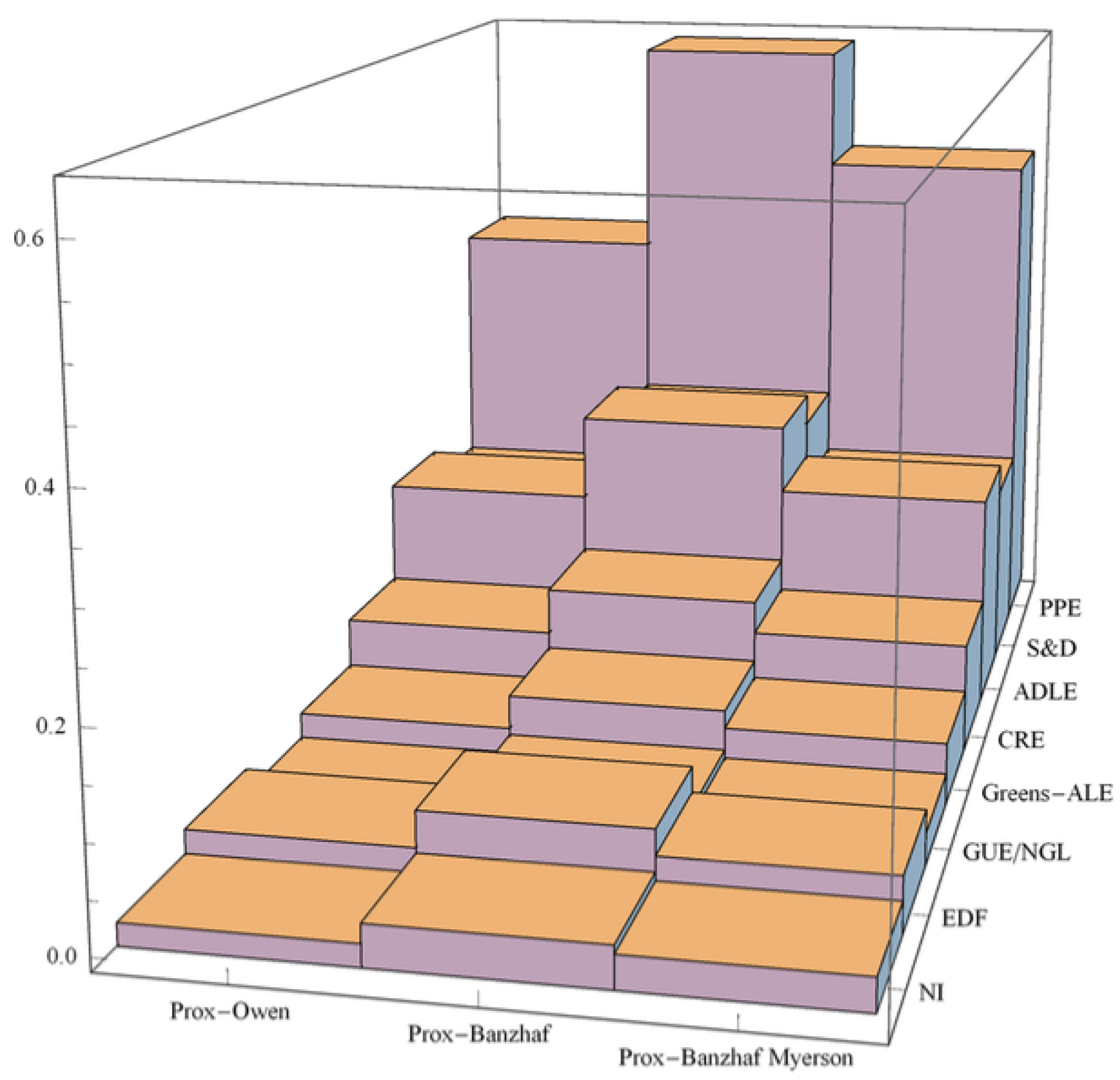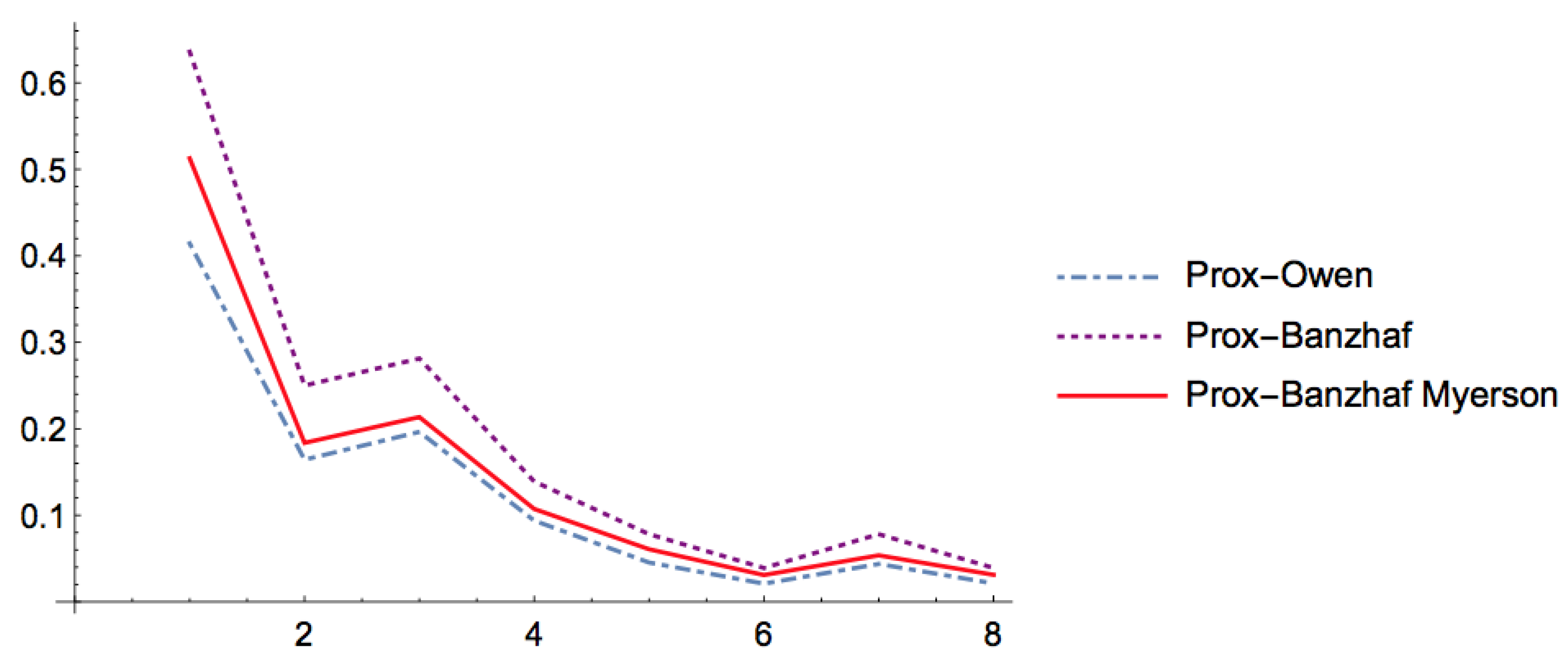Now, in Figure 4 and Figure 5, we compare for this example the three known indices for games with a proximity relation among the agents (the prox-Owen value [9], the prox-Banzhaf value [10] and the prox-Banzhaf–Myerson value. Observe that, besides getting a different theoretical approximation for the problem, the new solution obtain a moderate option between the others. They get the same results in the qualitative sense, but they obtain quantitative difference. The quantitive indices are used for instance to allocate the seats in specific committees of a chamber. They are distributed proportionally to the index, so a difference in the quantitative power can mean a difference in the number of seats of each group in these committees.

7. Conclusions

In this paper, a new solution for cooperative games with a proximity relation among the players was introduced, This outcome is a new version of Banzhaf value for these situations satisfying a fuzzy property based in the group symmetry. We showed in Section 6 that the prox-Banzhaf–Myerson value obtains a power distribution between the prox-Owen and the prox-Banzhaf values.

References

- Shapley, L.S. A value for N-Person Games. In Contributions to the Theory of Games; Kuhn, H.W., Tucker, A.W., Eds.; Princeton University Press: Princeton, NJ, USA, 1953; Volume 2, pp. 307–317. [Google Scholar]
- Banzhaf, J.F. Weighted voting doesn’t work. Rutgers Law Rev. 1965, 19, 317–343. [Google Scholar]
- Dubey, P.; Shapley, L.S. Mathematical Properties of the Banzhaf Power Index. Math. Oper. Res. 1979, 4, 99–131. [Google Scholar] [CrossRef]
- Aumann, R.J.; Dreze, J.H. Cooperative games with coalition structures. Int. J. Game Theory 1974, 3, 217–237. [Google Scholar] [CrossRef]
- Myerson, R.B. Graphs and cooperation in games. Math. Oper. Res. 1977, 2, 225–229. [Google Scholar] [CrossRef]
- Owen, G. Values of games with a priori unions. Math. Econ. Game Theory Lect. Notes Econ. Math. Syst. 1977, 141, 76–88. [Google Scholar]
- Alonso-Meijide, J.M.; Fiestras-Janeiro, M.G. Modification of the Banzhaf Value for Games with a Coalition Structure. Ann. Oper. Res. 2002, 109, 213–227. [Google Scholar] [CrossRef]
- Casajus, A. Beyond Basic Structures in Game Theory. Ph.D. Thesis, University of Leipzig, Leipzig, Germany, 2007. [Google Scholar]
- Fernández, J.R.; Gallego, I.; Jiménez-Losada, A.; Ordóñez, M. Cooperation among agents with a proximity relation. Eur. J. Oper. Res. 2016, 250, 555–565. [Google Scholar] [CrossRef]
- Fernández, J.R.; Gallego, I.; Jiménez-Losada, A.; Ordóñez, M.A. Banzhaf value for games with a proximity relation among the agents. Int. Approx. Reason. 2017, 88, 192–208. [Google Scholar] [CrossRef]
- Aubin, J.P. Cooperative fuzzy games. Math. Oper. Res. 1981, 6, 1–13. [Google Scholar] [CrossRef]
- Tsurumi, M.; Tanino, T.; Inuiguchi, M. A Shapley function on a class of cooperative fuzzy games. Eur. J. Oper. Res. 2001, 129, 596–618. [Google Scholar] [CrossRef]
- Choquet, G. Theory of Capacities. Ann. Inst. Fourier 1953, 5, 131–295. [Google Scholar] [CrossRef] [Green Version]
- Jiménez-Losada, A.; Fernández, J.R.; Ordóñez, M.; Grabisch, M. Games on fuzzy communication structures with Choquet players. Eur. J. Oper. Res. 2010, 207, 836–847. [Google Scholar] [CrossRef]
- Gallego, I.; Fernández, J.R.; Jiménez-Losada, A.; Ordóñez, M. A Banzhaf value for games with fuzzy communication structure: Computing the power of the political groups in the European Parliament. Fuzzy Sets Syst. 2014, 255, 128–145. [Google Scholar] [CrossRef]
- Jiménez-Losada, A.; Fernández, J.R.; Ordóñez, M. Myerson values for games with fuzzy communication structures. Fuzzy Sets Syst. 2013, 213, 74–90. [Google Scholar] [CrossRef]
- Mordeson, J.N.; Nair, P.S. Fuzzy Graphs and Fuzzy Hypergraphs; Studies in Fuzziness and Soft Computing 46; Physica-Verlag: Heidelberg, Germany, 2000. [Google Scholar]
© 2020 by the authors. Licensee MDPI, Basel, Switzerland. This article is an open access article distributed under the terms and conditions of the Creative Commons Attribution (CC BY) license (http://creativecommons.org/licenses/by/4.0/).