Unsupervised Hashing with Gradient Attention


Abstract
:1. Introduction
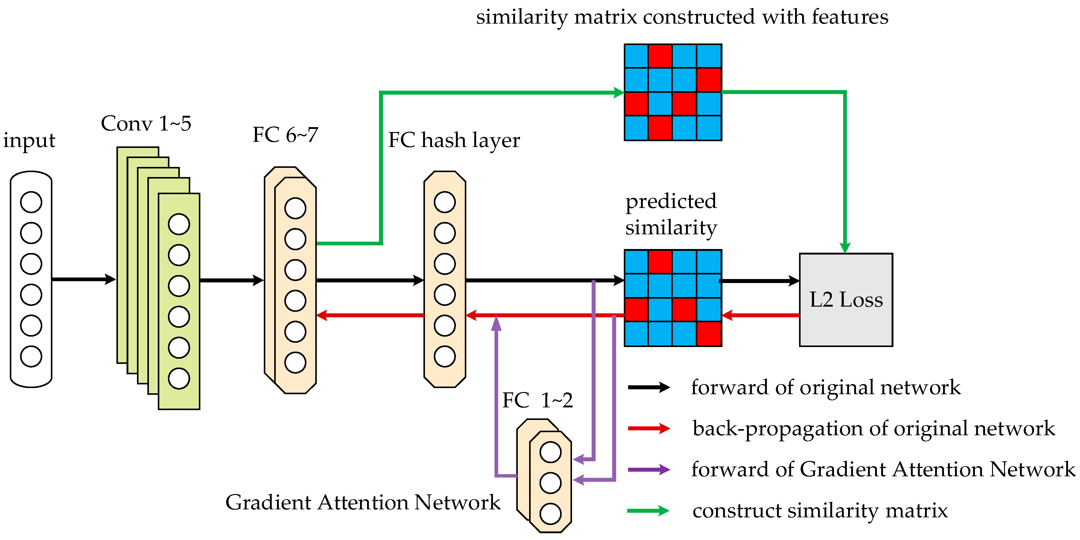
2. UHGA Mmethod
2.1. Deep Hash Model
2.2. The Dilemma of Gradient Decline
2.3. Gradient Attention Network
| Algorithm 1. UHGA |
| Input: |
| Training set ; |
| Code length k; |
| Output: |
| Updated network parameters and hash codes . |
| Initialization: |
| Initialize the Alexnet; |
| Initialize parameters from the pre-trained Alexnet. |
| Extracting features of Alexnet FC-7 layer. |
| Using (2) to calculate cosine distance of paired image features. |
| Using (3) to construct similarity matrix . |
| Repeat |
| a mini batch of images from , and for each image , follow each step below: |
| •Calculate and obtain the derivative in the process of backpropagation; |
| •Using , and as input of gradient attention network to calculate attention weights ; |
| •Calculate and by (16) and (17); |
| •Calculate the new derivatives and obtain gradient of as in the process of backpropagation; |
| •Update by (18); |
| •Calculate the loss after update; |
| •Update ; |
| •; |
| Until number of iterations reached |
2.4. Optimization
3. Experimental Results and Analysis
3.1. Datasets, Evaluation Metrics and Benchmarks
- (1)
- CIFAR-10. A total of 60,000 images, including 10 categories, and each category contains 6000 images, which is a single-label dataset.
- (1)
- NUS-WIDE. A total of 269,648 images, including 21 categories, each category is associated with at least 5000 images and each image belongs to one or more categories, which is a multi-label dataset.
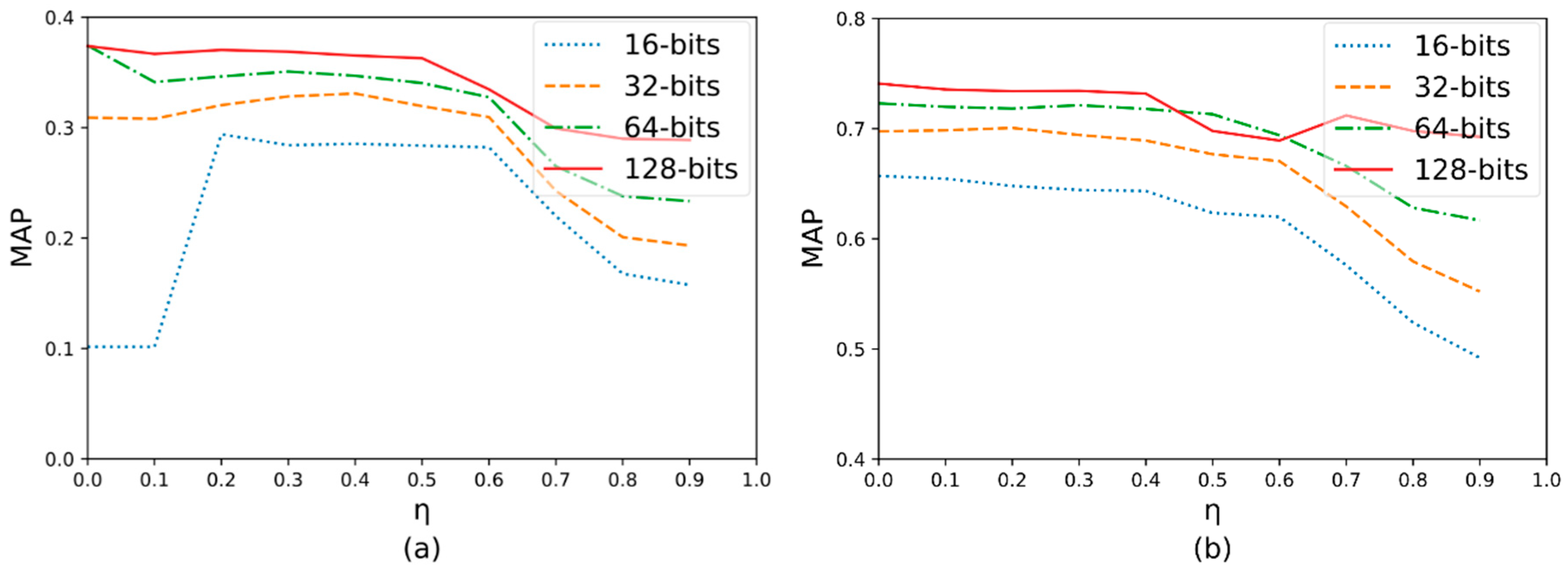
3.2. Hyperparameter Analysis
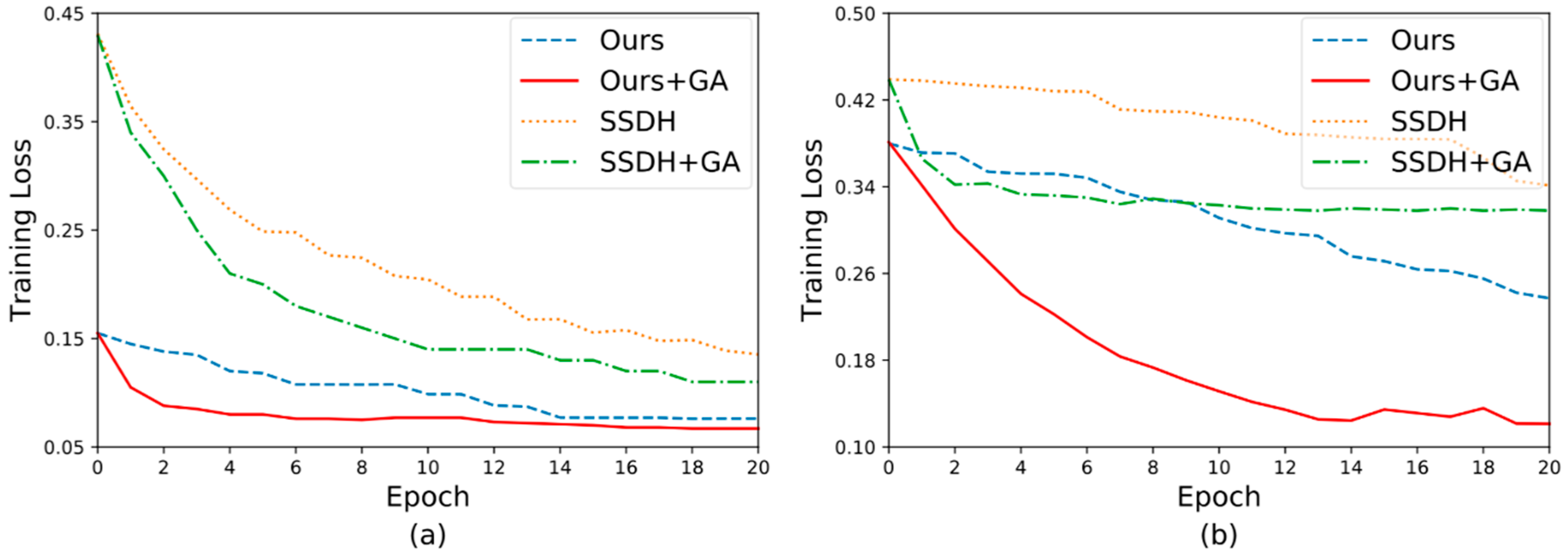
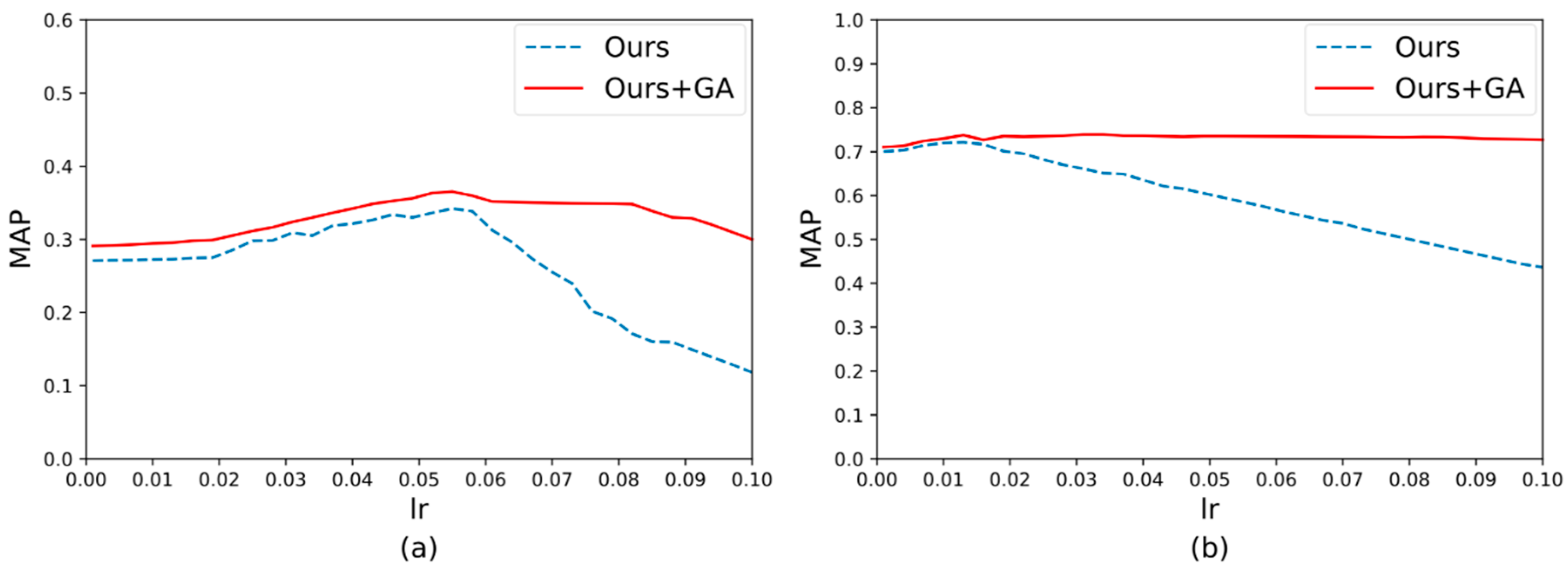
3.3. The effect of Gradient Attention
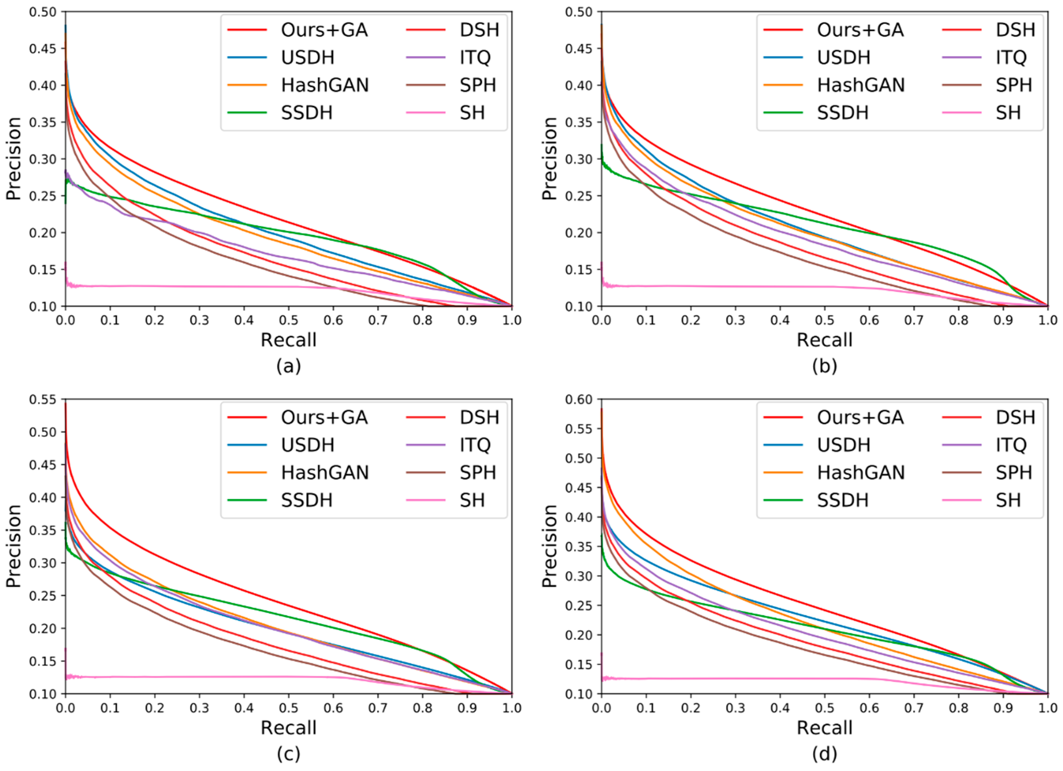
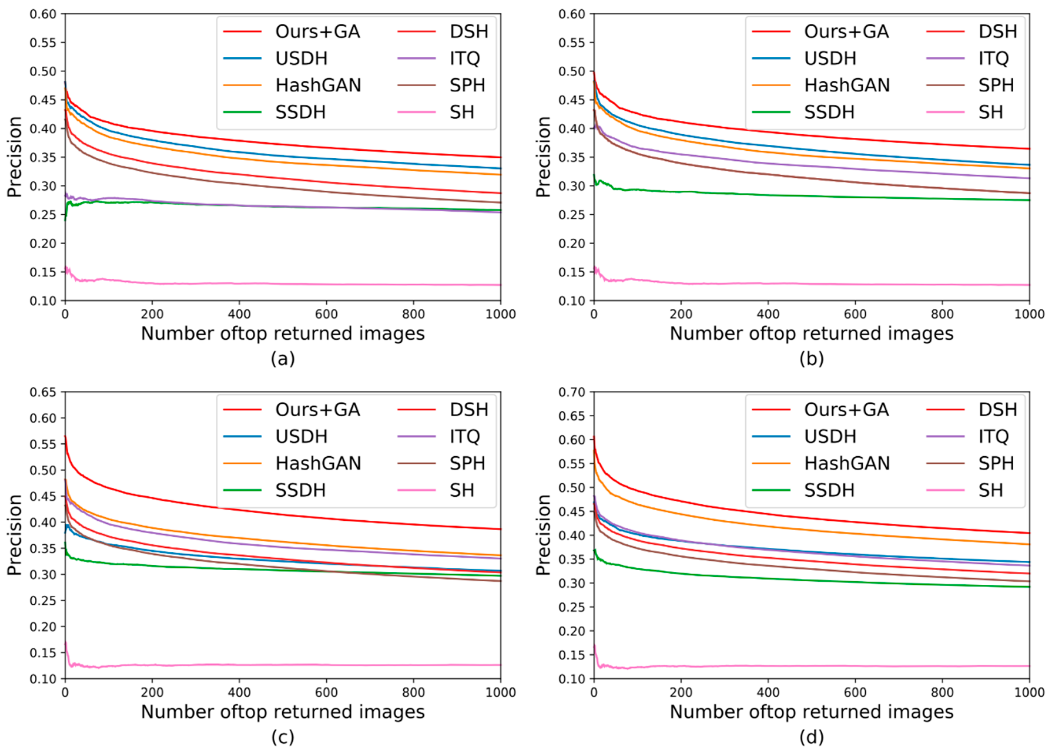
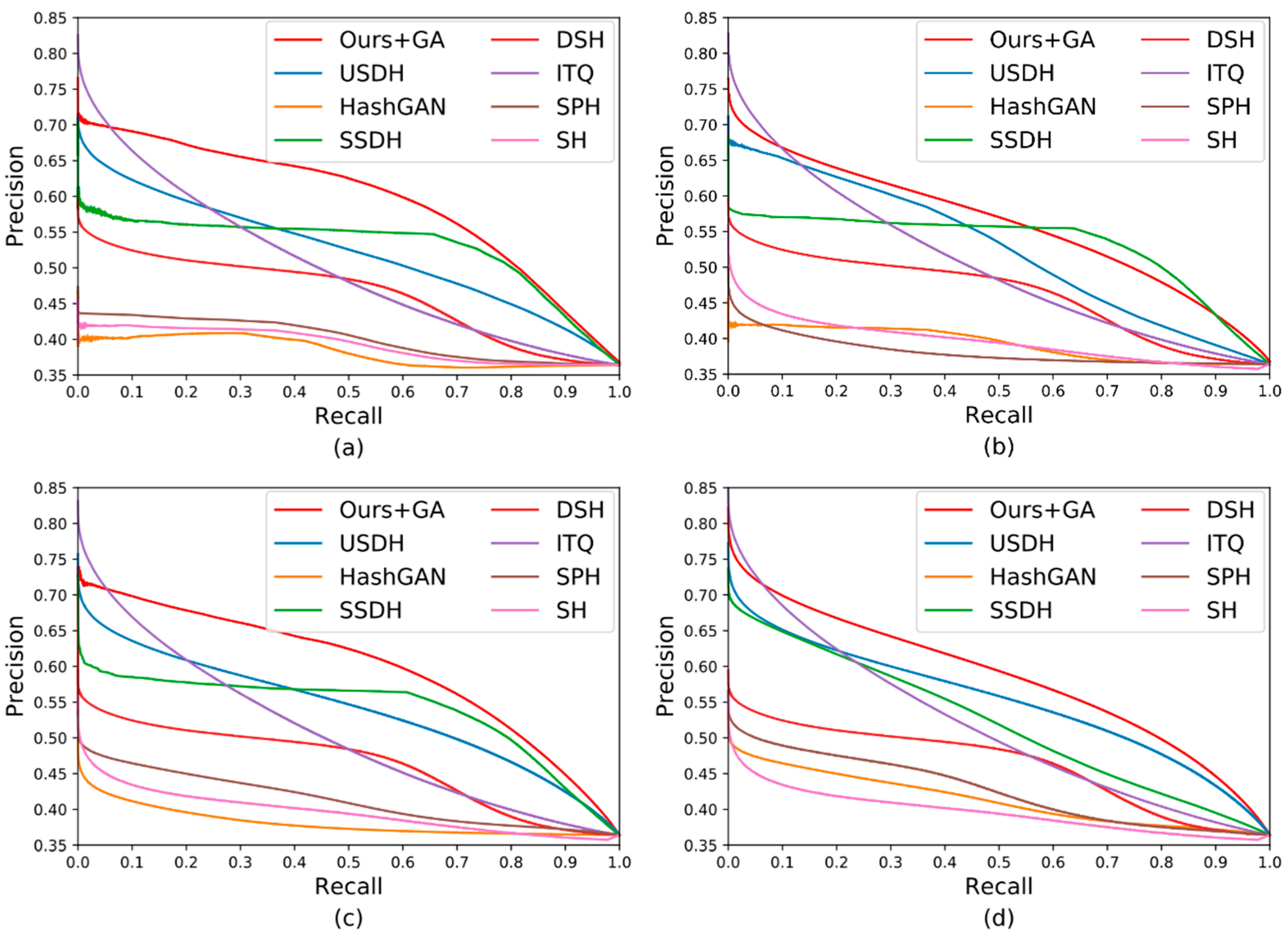
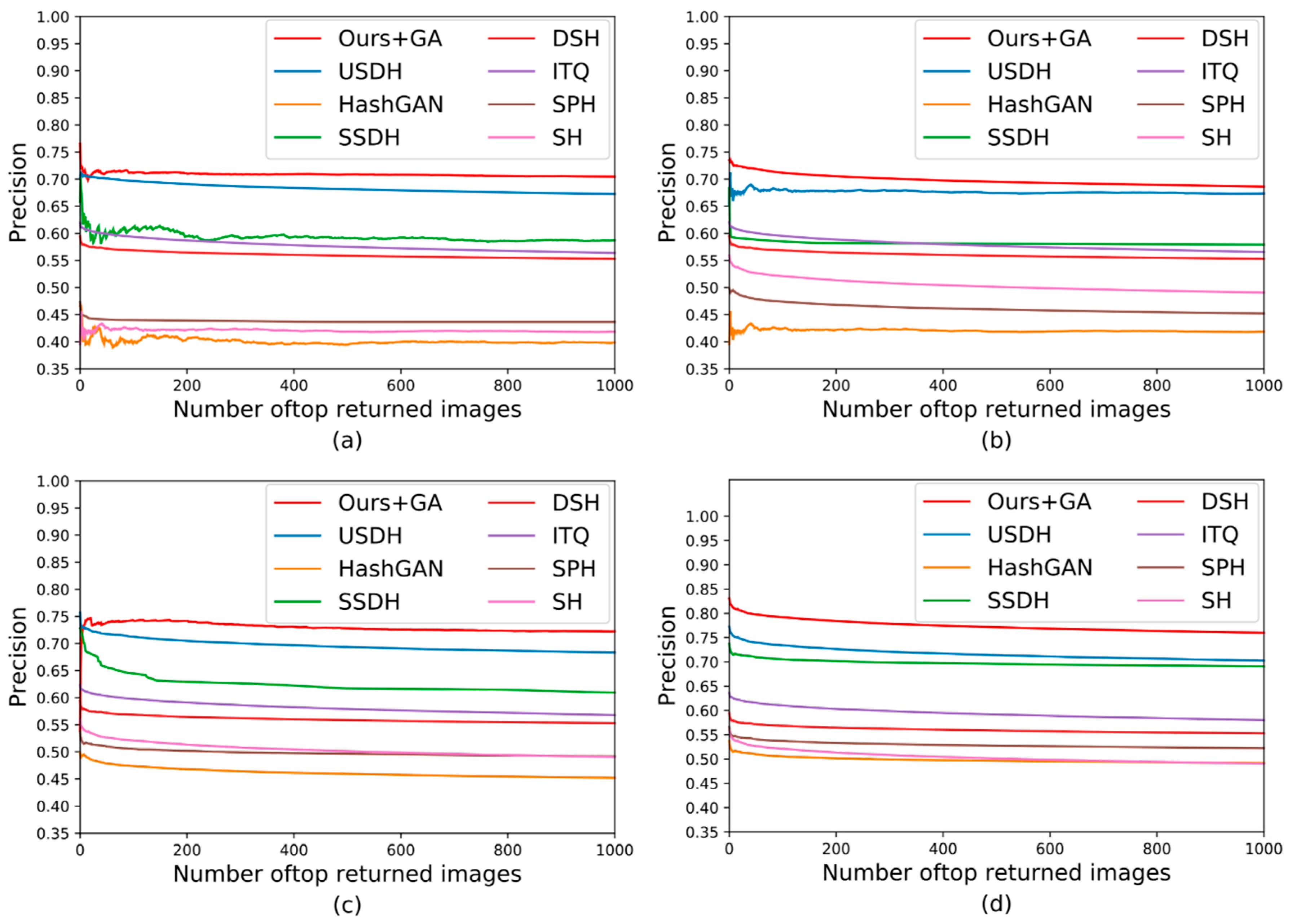
3.4. Comparison of Experimental Results
4. Conclusions
Author Contributions
Funding
Conflicts of Interest
References
- Liu, Y.; Zhang, D.; Lu, G.; Ma, W.Y. A survey of content-based image retrieval with high-level semantics. Pattern Recognit. 2007, 40, 262–282. [Google Scholar] [CrossRef]
- Tang, J.; Li, Z.; Wang, M.; Zhao, R. Neighborhood discriminant hashing for large-scale image retrieval. IEEE Trans. Image Process. 2015, 24, 2827–2840. [Google Scholar] [CrossRef] [PubMed]
- Paulevé, L.; Jégou, H.; Amsaleg, L. Locality sensitive hashing: A comparison of hash function types and querying mechanisms. Pattern Recognit. Lett. 2010, 31, 1348–1358. [Google Scholar] [CrossRef] [Green Version]
- Andoni, A.; Indyk, P. Near-optimal hashing algorithms for approximate nearest neighbor in high dimensions. In Proceedings of the Annual IEEE Symposium on Foundations of Computer Science (FOCS’06), Berkeley, CA, USA, 22–24 October 2006; Volume 47, pp. 459–468. [Google Scholar]
- Zhang, D.; Wang, J.; Cai, D.; Lu, J. Self-taught hashing for fast similarity search. In Proceedings of the 33rd international ACM SIGIR Conference on Research and Development in Information Retrieval, Geneva, Switzerland, 19–23 July 2010; Association for Computing Machinery: New York, NY, USA, 2010; pp. 18–25. [Google Scholar]
- He, K.; Wen, F.; Sun, J. K-means hashing: An affinity-preserving quantization method for learning binary compact codes. In Proceedings of the 2015 IEEE Conference on Computer Vision and Pattern Recognition (CVPR), Portland, OG, USA, 25–27 June 2013; pp. 2938–2945. [Google Scholar]
- Shen, F.; Zhou, X.; Yang, Y.; Song, J.; Shen, H.T.; Tao, D. A fast optimization method for general binary code learning. IEEE Trans. Image Process. 2016, 25, 5610–5621. [Google Scholar] [CrossRef] [PubMed]
- Xu, H.; Wang, J.; Li, Z.; Zeng, G.; Li, S.; Yu, N. Complementary hashing for approximate nearest neighbor search. In Proceedings of the 2011 International Conference on Computer Vision (ICCV), Barcelona, Spain, 6–13 November 2011; pp. 1631–1638. [Google Scholar]
- Wang, J.; Liu, W.; Kumar, S.; Chang, S.F. Learning to hash for indexing big data—A survey. Proc. IEEE 2015, 104, 34–57. [Google Scholar] [CrossRef]
- Wang, J.; Zhang, T.; Sebe, N.; Shen, H.T. A survey on learning to hash. IEEE Trans. Pattern Anal. Mach. Intell. 2017, 40, 769–790. [Google Scholar] [CrossRef]
- Roweis, S.T.; Saul, L.K. Nonlinear dimensionality reduction by locally linear embedding. Science 2000, 290, 2323–2326. [Google Scholar] [CrossRef] [Green Version]
- Bai, X.; Yang, H.; Zhou, J.; Ren, P.; Cheng, J. Data-dependent hashing based on p-stable distribution. IEEE Trans. Image Process. 2014, 23, 5033–5046. [Google Scholar] [CrossRef] [Green Version]
- Gong, Y.; Lazebnik, S.; Gordo, A.; Perronnin, F. Iterative quantization: A procrustean approach to learning binary codes for large-scale image retrieval. IEEE Trans. Pattern Anal. Mach. Intell. 2012, 35, 2916–2929. [Google Scholar] [CrossRef] [Green Version]
- Shen, F.; Shen, C.; Liu, W.; Shen, H.T. Supervised Discrete Hashing. In Proceedings of the 2015 IEEE Conference on Computer Vision and Pattern Recognition (CVPR), Boston, MA, USA, 7–12 June 2015; pp. 37–45. [Google Scholar]
- Cao, Z.; Long, M.; Wang, J.; Yu, P.S. Hashnet: Deep learning to hash by continuation. In Proceedings of the IEEE International Conference on Computer Vision (ICCV), Venice, Italy, 22–29 October 2017; pp. 5608–5617. [Google Scholar]
- Yang, H.F.; Lin, K.; Chen, C.S. Supervised learning of semantics-preserving hash via deep convolutional neural networks. IEEE Trans. Pattern Anal. Mach. Intell. 2017, 40, 437–451. [Google Scholar] [CrossRef] [Green Version]
- Liu, H.; Wang, R.; Shan, S.; Chen, X. Deep supervised hashing for fast image retrieval. In Proceedings of the 2016 IEEE Conference on Computer Vision and Pattern Recognition (CVPR), Las Vegas, NV, USA, 26 June–1 July 2016; pp. 2064–2072. [Google Scholar]
- Li, W.J.; Wang, S.; Kang, W.C. Feature learning based deep supervised hashing with pairwise labels. In Proceedings of the 2015 International Joint Conference on Artificial Intelligence (IJCAI), Buenos Aires, Argentina, 28 July–1 August 2015; pp. 1711–1717. [Google Scholar]
- Li, Q.; Sun, Z.; He, R.; Tan, T. Deep supervised discrete hashing. In Advances in Neural Information Processing Systems; Curran Associates: New York, USA, 2017; pp. 2482–2491. [Google Scholar]
- Wang, D.; Wang, L. On OCT image classification via deep learning. IEEE Photonics J. 2019, 11, 1–14. [Google Scholar] [CrossRef]
- Wu, Y.; Sun, Q.; Hou, Y.; Zhang, J.; Zhang, Q.; Wei, X. Deep covariance estimation hashing. IEEE Access 2019, 7, 113223–113234. [Google Scholar] [CrossRef]
- Cakir, F.; He, K.; Bargal, S.A.; Sclaroff, S. Hashing with mutual information. IEEE Trans. Pattern Anal. Mach. Intell. 2019, 41, 2424–2437. [Google Scholar] [CrossRef] [Green Version]
- Li, N.; Li, C.; Deng, C.; Liu, X.; Gao, G. Deep joint semantic-embedding hashing. In Proceedings of the Twenty-Seventh International Joint Conference on Artificial Intelligence (IJCAI-18), Stockholm, Sweden, 13–19 July 2018; pp. 2397–2403. [Google Scholar]
- Cheng, S.; Wang, L.; Du, A. An adaptive and asymmetric residual hash for fast image retrieval. IEEE Access 2019, 7, 78942–78953. [Google Scholar] [CrossRef]
- Du, A.; Wang, L.; Cheng, S.; Ao, N. A Privacy-Protected Image Retrieval Scheme for Fast and Secure Image Search. Symmetry 2020, 12, 282. [Google Scholar] [CrossRef] [Green Version]
- Cheng, S.L.; Wang, L.J.; Huang, G.; Du, A.Y. A privacy-preserving image retrieval scheme based secure kNN, DNA coding and deep hashing. Multimed. Tools Appl. 2019. [Google Scholar] [CrossRef]
- Li, J. Context-based image re-ranking for content-based image retrieval. In Proceedings of the 2011 IEEE Symposium on Computational Intelligence for Multimedia, Signal and Vision Processing, Paris, France, 11–15 April 2011; pp. 39–46. [Google Scholar]
- Salakhutdinov, R.; Hinton, G. Semantic hashing. Int. J. Approx. Reason. 2009, 50, 969–978. [Google Scholar] [CrossRef] [Green Version]
- Erin Liong, V.; Lu, J.; Wang, G.; Moulin, P.; Zhou, J. Deep hashing for compact binary codes learning. In Proceedings of the 2015 IEEE Conference on Computer Vision and Pattern Recognition (CVPR), Boston, MA, USA, 7–12 June 2015; pp. 2475–2483. [Google Scholar]
- Lin, K.; Lu, J.; Chen, C.S.; Zhou, J. Learning compact binary descriptors with unsupervised deep neural networks. In Proceedings of the 2016 IEEE Conference on Computer Vision and Pattern Recognition (CVPR), Las Vegas, NV, USA, 26 June–1 July 2016; pp. 1183–1192. [Google Scholar]
- Jin, S.; Yao, H.; Sun, X.; Zhou, S. Unsupervised semantic deep hashing. Neurocomputing 2019, 351, 19–25. [Google Scholar] [CrossRef] [Green Version]
- Yang, E.; Deng, C.; Liu, T.; Liu, W.; Tao, D. Semantic structure-based unsupervised deep hashing. In Proceedings of the Twenty-Seventh International Joint Conference on Artificial Intelligence (IJCAI-18), Stockholm, Sweden, 13–19 July 2018; pp. 1064–1070. [Google Scholar]
- Li, C.; Wang, L.; Cheng, S.; Ao, N. Generative Adversarial Network-Based Super-Resolution Considering Quantitative and Perceptual Quality. Symmetry 2020, 12, 449. [Google Scholar] [CrossRef] [Green Version]
- Ghasedi Dizaji, K.; Zheng, F.; Sadoughi, N.; Yang, Y.; Deng, C.; Huang, H. Unsupervised deep generative adversarial hashing network. In Proceedings of the IEEE International Conference on Computer Vision (ICCV), Coimbatore, India, 21–22 September 2018; pp. 3664–3673. [Google Scholar]
- Deng, C.; Yang, E.; Liu, T.; Li, J.; Liu, W.; Tao, D. Unsupervised semantic-preserving adversarial hashing for image search. IEEE Trans. Image Process. 2019, 28, 4032–4044. [Google Scholar] [CrossRef]
- Huang, L.K.; Chen, J.; Pan, S.J. Accelerate learning of deep hashing with gradient attention. In Proceedings of the IEEE International Conference on Computer Vision (ICCV), Seoul, Korea, 27 October–2 November 2019; pp. 5271–5280. [Google Scholar]
- Weiss, Y.; Torralba, A.; Fergus, R. Spectral hashing. In Advances in Neural Information Processing Systems; The MIT Press: Cambridge, MA, USA, 2009; pp. 1753–1760. [Google Scholar]
- Heo, J.P.; Lee, Y.; He, J.; Chang, S.F.; Yoon, S.E. Spherical hashing. In Proceedings of the 2012 IEEE Conference on Computer Vision and Pattern Recognition (CVPR), Providence, RI, USA, 16–21 June 2012; pp. 2957–2964. [Google Scholar]
- Jin, Z.; Li, C.; Lin, Y.; Cai, D. Density sensitive hashing. IEEE Trans. Cybern. 2013, 44, 1362–1371. [Google Scholar] [CrossRef] [PubMed] [Green Version]


| Item | Configuration |
|---|---|
| OS GPU | Ubuntu 16.04 (X64) 4*GTX 1080ti |
| CIFAR-10 (MAP@ALL) (bits) | NUS-WIDE (MAP@5000) (bits) | |||||||
|---|---|---|---|---|---|---|---|---|
| 16 | 32 | 64 | 128 | 16 | 32 | 64 | 128 | |
| 0 | 0.1015 | 0.3091 | 0.3744 | 0.3739 | 0.6571 | 0.6976 | 0.7230 | 0.7409 |
| 0.1 | 0.1015 | 0.3080 | 0.3413 | 0.3668 | 0.6546 | 0.6985 | 0.7198 | 0.7356 |
| 0.2 | 0.2940 | 0.3204 | 0.3464 | 0.3704 | 0.6480 | 0.7007 | 0.7183 | 0.7340 |
| 0.3 | 0.2841 | 0.3283 | 0.3508 | 0.3688 | 0.6444 | 0.6943 | 0.7213 | 0.7343 |
| 0.4 | 0.2854 | 0.3309 | 0.3470 | 0.3653 | 0.6434 | 0.6892 | 0.7179 | 0.7318 |
| 0.5 | 0.2837 | 0.3195 | 0.3404 | 0.3629 | 0.6235 | 0.6768 | 0.7131 | 0.6979 |
| 0.6 | 0.2822 | 0.3096 | 0.3276 | 0.3347 | 0.6199 | 0.6705 | 0.6940 | 0.6892 |
| 0.7 | 0.2199 | 0.2428 | 0.2650 | 0.2993 | 0.5761 | 0.6294 | 0.6661 | 0.7120 |
| 0.8 | 0.1677 | 0.2008 | 0.2380 | 0.2900 | 0.5239 | 0.5795 | 0.6282 | 0.6979 |
| 0.9 | 0.1576 | 0.1932 | 0.2334 | 0.2888 | 0.4920 | 0.5522 | 0.6168 | 0.6926 |
| Method | CIFAR-10 (MAP @ALL) (bits) | NUS-WIDE (MAP @5000) (bits) | ||||||
|---|---|---|---|---|---|---|---|---|
| 16 | 32 | 64 | 128 | 16 | 32 | 64 | 128 | |
| SSDH [32] | 0.2172 | 0.2313 | 0.2405 | 0.2351 | 0.5860 | 0.5788 | 0.6079 | 0.6127 |
| SSDH+GA | 0.2827 | 0.3018 | 0.3219 | 0.3462 | 0.6528 | 0.6637 | 0.6787 | 0.7032 |
| Ours | 0.2704 | 0.3133 | 0.3240 | 0.3452 | 0.6512 | 0.6846 | 0.7039 | 0.7125 |
| Ours+GA | 0.2936 | 0.3233 | 0.3499 | 0.3661 | 0.6601 | 0.6981 | 0.7224 | 0.7359 |
| Method | CIFAR-10 (MAP @ALL) (bits) | NUS-WIDE (MAP @5000) (bits) | ||||||
|---|---|---|---|---|---|---|---|---|
| 16 | 32 | 64 | 128 | 16 | 32 | 64 | 128 | |
| SH [37] | 0.1621 | 0.1575 | 0.1549 | 0.1548 | 0.4350 | 0.4129 | 0.4042 | 0.4100 |
| SPH [38] | 0.1664 | 0.1745 | 0.1931 | 0.1992 | 0.4458 | 0.4537 | 0.4926 | 0.5.00 |
| ITQ [13] | 0.1999 | 0.2098 | 0.2229 | 0.2312 | 0.5082 | 0.5139 | 0.5252 | 0.5311 |
| DSH [39] | 0.1686 | 0.1846 | 0.1955 | 0.2071 | 0.5123 | 0.5118 | 0.5110 | 0.5267 |
| SSDH [32] | 0.2172 | 0.2313 | 0.2405 | 0.2351 | 0.5860 | 0.5788 | 0.6079 | 0.6127 |
| HashGAN [34] | 0.2457 | 0.2678 | 0.3077 | 0.3422 | 0.4020 | 0.4207 | 0.4460 | 0.4883 |
| USDH [31] | 0.2613 | 0.3021 | 0.3122 | 0.3241 | 0.6407 | 0.6568 | 0.6587 | 0.6724 |
| Ours+GA | 0.2936 | 0.3233 | 0.3499 | 0.3661 | 0.6601 | 0.6981 | 0.7224 | 0.7359 |
© 2020 by the authors. Licensee MDPI, Basel, Switzerland. This article is an open access article distributed under the terms and conditions of the Creative Commons Attribution (CC BY) license (http://creativecommons.org/licenses/by/4.0/).
Share and Cite
Jiang, S.; Wang, L.; Cheng, S.; Du, A.; Li, Y. Unsupervised Hashing with Gradient Attention. Symmetry 2020, 12, 1193. https://doi.org/10.3390/sym12071193
Jiang S, Wang L, Cheng S, Du A, Li Y. Unsupervised Hashing with Gradient Attention. Symmetry. 2020; 12(7):1193. https://doi.org/10.3390/sym12071193
Chicago/Turabian StyleJiang, Shaochen, Liejun Wang, Shuli Cheng, Anyu Du, and Yongming Li. 2020. "Unsupervised Hashing with Gradient Attention" Symmetry 12, no. 7: 1193. https://doi.org/10.3390/sym12071193