Testing of a Virtualized Distributed Processing System for the Execution of Bio-Inspired Optimization Algorithms

Abstract

Due to the stochastic characteristics of bio-inspired optimization algorithms, several executions are often required; then a suitable infrastructure must be available to run these algorithms. This paper reviews a virtualized distributed processing scheme to establish an adequate infrastructure for the execution of bio-inspired algorithms. In order to test the virtualized distributed system, the well known versions of genetic algorithms, differential evolution and particle swarm optimization, are used. The results show that the revised distributed virtualized schema allows speeding up the execution of the algorithms without altering their result in the objective function.

1. Introduction

Artificial intelligence and processing technologies are important tools to improve the analysis of the different phenomena in nature; it is important to have an efficient infrastructure for data processing and analysis, which must be platform-independent [1]. In relation to one of the techniques used in artificial intelligence, bio-inspired optimization algorithms have proven to be a suitable tool for troubleshooting engineering; however, because of their stochastic behavior they often require a large number of iterations such as a number of executions to get a useful solution. Therefore, it is necessary to establish an adequate infrastructure to run such algorithms—a virtualized distributed system being a suitable option.

1.1. Bio-Inspired Optimization

Bio-inspired optimization techniques (heuristics) are a suitable alternative when traditional methods cannot determine appropriate results or have limitations. In the field of bio-inspired optimization, there are different proposals based on behaviors and phenomena that exist in nature [2]. In this regard, approaches of individuals among the algorithms are stochastic hill climbing (SHC) and simulated annealing (SA). Among the methods based on several individuals (populations), the genetic algorithms (GA), differential evolution (DE), ant colony optimization (ACO), bacterial chemotaxis (BCO), and particle swarm optimization (PSO). The stochastic hill climbing algorithm is based on the stochastic selection of neighboring solutions, which are accepted in cases wherein there is an improvement in the target function [3]. Simulated annealing is a method that emulates the crystalline formation of a material by heating and cooling it, seeking to move from a higher to a lower energy state [3]. Genetic algorithms and differential evolution seek to emulate the process of nature by improving a species over time [3]. On the other hand, algorithms based on ant colonies, bacterial chemotaxis, and swarms of particles are inspired by the behavior of living beings searching for food [4,5,6].

In order to test the processing system, we used the standard versions of genetic algorithms, differential evolution, and particle swarm optimization, which are widely known.

1.2. Distributed Processing Systems

Aggregate computing is an emerging approach to complex coordination engineering that results in distributed systems. This approach is based on the interactions of the visualization system in terms of information that is propagated across device groups and their interactions with their peers and environment [7]. Some applications that involve data analysis typically perform the calculations in a data center or cloud environment. As these applications grow in scale, this centralized approach leads to bandwidth requirements and potentially impractical computational latencies. This has generated interest in computing wherein processing is in a distributed manner [8].

According to [9], the development of this technology shows the importance of teaching the aspects of parallel computing. In this regard, the authors of [9] present a model for incorporating parallel and distributed computing (PDC) throughout an undergraduate computer science (CS) curriculum, presenting students with computer topics of distributed and parallel computation in the intermediate level.

Parallel and distributed computing is of importance when handling a large amount of data and the ability to process it; some applications of parallel computing are described below.

An application on renewable energy generation can be seen in [10], where a distributed data processing system is presented to improve the estimation of urban solar potential by directly using a dense set of scanning points obtained from aerial laser scans (ALS) that allow incorporating true, complex, and heterogeneous elements common in most urban areas.

Another application on renewable energy can be seen in [11], where a hybrid distributed computing system is used in Apache Spark for wind speed forecasting, which corresponds to an arduous task given the randomness of the wind speed. Using the distributed computing strategy, the system can divide large wind speed datasets into groups and use them in parallel.

In relation to a geomatics application, in [1] a distributed computer framework is provided, allowing data collection and processing. According to the authors, the proposed system can support efficient range queries and large-scale spatial data processing in a Spark cluster and another in Flink, providing an effective cross-platform distributed computing solution for fast processing of large-scale spatial data.

Finally, an application in the field of agriculture can be seen in [12], where it is necessary to evaluate the spatial distributions of crop yields under current and future climatic conditions. This task generally requires considerable effort in order to prepare the input data and post-process the results, which is why the authors developed a simulation support system to automate repetitive and tedious tasks using virtual machines connected over a local network, allowing for a clustered computer without workstations having to be dedicated.

1.3. Virtualization Systems

The concept of virtualization is applied in cloud computing systems to help users and owners achieve better use and efficient management of the cloud at the lowest cost [13]. Live migration of virtual machines (VM) is an essential feature of virtualization, allowing one to migrate virtual machines from one location to another without suspending them. This process has many advantages for data centers, such as load balancing, inline maintenance, power management, and proactive fault tolerance [13]. When a system such as a processor, memory, or I/O device is virtualized, its interface and all visible resources are mapped to a virtual interface in such a way that the actual system is transformed into a different virtual or even a set of multiple virtual systems [14]. Virtualization technologies allow decoupling the architecture and user-perceived behavior of hardware and software resources from the physical deployment [15].

According to [16], virtualization has made it possible to completely isolate virtual machines from each other. When applications running inside virtual machines have real-time restrictions, threads that deploy virtual cores must be programmed in a predictable way over physical cores. Meanwhile, reference [17] states that real-time virtual machines are suitable for tightly coupled computer systems wherein tasks are executed from the associated language. Here is an approach to support the transfer of tasks between freely attached computers in a real-time environment to add more features without updating the software.

Essentially, energy consumption is an important aspect of virtualization; in line with [18], the high power consumption of cloud data centers presents a significant challenge from both an economic and environmental perspective. Server consolidation using virtualization technology is widely used to reduce the power consumption rates of data centers. The efficient virtual machine placement (VMP) of virtual machines plays an important role in server consolidation technology, this being a difficult problem of type NP (nondeterministic polynomial time) for which the optimal solutions are not possible. In addition, reference [19] states that the assignment of a virtual to a physical machine affects the power consumption, manufacturing, and downtime of physical machines. According to [20], the demand for power for cloud data centers has increased markedly; therefore, the consolidation of dynamic virtual machines, as one of the effective methods to reduce energy consumption, is widely used in large data centers in the cloud.

On energy-related work, a hybrid VMP algorithm based on an improved genetic algorithm using permutation and a multidimensional resource allocation strategy is proposed in [18]. The proposed VMP algorithm aims to improve the rate of high power consumption of cloud data centers by minimizing the number of active servers that host virtual machines; it also seeks to achieve balanced use of resources (CPU, RAM, and bandwidth) of active servers, which in turn reduces wasted resources. Meanwhile, in [19], the problem is formulated as an optimization of packaging to minimize the energy costs of operating machines and inactive machines. When considering the CPU and memory requirements of a virtual machine, the allocation is limited by the capabilities of the physical machine. Another work can be seen in [20], where, in order to efficiently ensure quality of service (QoS), a VM approach is proposed that considers the current and future uses of resources through host overload detection.

1.4. Document Organization

Distributed processing and virtualization technologies are suitable tools when computing power is needed, as is the case with bio-inspired optimization algorithms, as their stochastic characteristics require running several times with different settings of their parameters. Therefore, this paper reviews a virtualized parallel processing scheme for the execution of bio-inspired optimization algorithms. The document is organized as follows. The first part reviews concepts on distributed computer systems and virtualization, and also presents the computer system used; then it describes the optimization of bio-inspired algorithms and the test functions considered, and subsequently presents the statistical results obtained, showing the configurations of the algorithms; finally, the conclusions of the work are established.

The objective of this work was to evaluate the virtualized distributed processing system located at the High Performance Computing Center (Centro de Computación de Alto Desempeño—CECAD) of the Universidad Distrital Francisco José de Caldas (UDFJC) which provides a distributed computing service in a virtualized way to the researchers of the UDFJC. The aim was to look at the characteristics of this system for the execution of bio-inspired optimization algorithms and the advantages that it has in relation to processing time.

2. Distributed Processing Systems

According to [21], a distributed system is a collection of autonomous computer elements (nodes) visible to users as a single consistent system. Each of the computer elements can behave independently and can be hardware devices or a software process. In this way, users (people or applications) think they are dealing with a single system; this implies that collaboration between nodes must be presented, which is an important aspect in the development of distributed systems [21]. A distributed system must have the following features to provide maximum performance to users:

Openness: This attribute ensures that a subsystem is continuously open to interaction with other systems, such as those designed to perform inter-machine interactions over a network by allowing distributed systems to expand and scale.

Scalable: A distributed system can function properly even if some aspect of the system scales to a larger size. Three components should be considered: the number of users and other entities that are part of the system, the distance between the farthest nodes of the system, and the number of organizations that exercise administrative control over parts of the system.

Predictable performance: Predictable performance is the ability to provide the desired responsiveness in a timely manner, according to a performance metric that may be the response time associated with the time elapsed between a query in a computer system and response. Another metric corresponds to the rate at which a network sends or receives data. Metrics associated with system utilization and network capacity can also be used to establish the performance.

Security: Security features are primarily intended to provide confidentiality, integrity, and availability; thus, distributed systems must allow communication between programs, users, and resources on different computers by applying the necessary security tools.

Fault-tolerant: Distributed systems consist of a large number of hardware and software modules that can fail in the long-term. Such component failures can result in a lack of service. Therefore, systems should be able to recover from component failures without performing erroneous actions.

Transparency: Distributed systems should be perceived by users and application developers as a whole and not as a collection of cooperating components. In this way, for the user the locations of the computer systems involved in the operations, data replication, failures, system recovery, etc., are not visible.

Types of Parallel Architecture

On the classification of parallel architectures, Michael Flynn proposed a taxonomy that simplified the categorization of different classes of architectures and control methods based on the relationships of data and instruction (control) with respect to the parallelism of the data flow [22,23].

There are different ways CPUs can be connected together; Flynn’s classification considers machines by the number of instruction flows and the number of data flows. Multiple instruction sequences mean that different statements can be executed simultaneously [22,23]. Data flows refer to memory operations whose four combinations are:

• SISD (single instruction stream, single data stream): This classification corresponds to the traditional single-processor computer. It represents the conventional sequential (serial) processor structure where a single control thread, the flow of instructions, guides the sequence of operations performed on a single data set, one operating at a time.
• SIMD (single instruction stream, multiple data streams): This architecture supports multiple streams of data to be processed simultaneously by replicating computer hardware. Single statement means that all data streams are processed using the same calculation logic. It can be seen as an array processor, where a single instruction operates in many data units in parallel.
• MISD (multiple instruction stream, single data stream): Corresponds to a rare architecture, which operates in a single data flow but has multiple computing engines that use the same data flow. That is multiple processors, each with their own flow of instructions, working on the same data with which all the other processors operate. They could be used to provide fault tolerance with heterogeneous systems operating with the same data.
• MIMD (multiple instruction stream, multiple data stream): This is the most generic parallel processing architecture where any type of distributed application is programmed. Multiple stand-alone processors running in parallel work in separate data flows. The logic of the applications running on these processors can also be very different. All distributed systems are recognized as MIMD architectures. At any time, a lot of operations are performed, but they do not have to be the same and are mostly different.

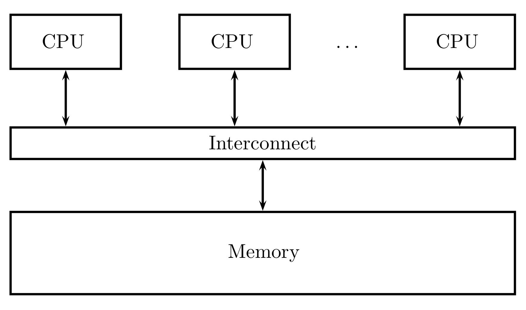
Shared memory and distributed memory systems are two main types of MIMD. In a shared memory system (Figure 1), a collection of stand-alone processors is connected to a memory system over an interconnected network, and each processor can access each memory location. In a shared memory system, processors are usually implicitly communicated by accessing shared data structures.

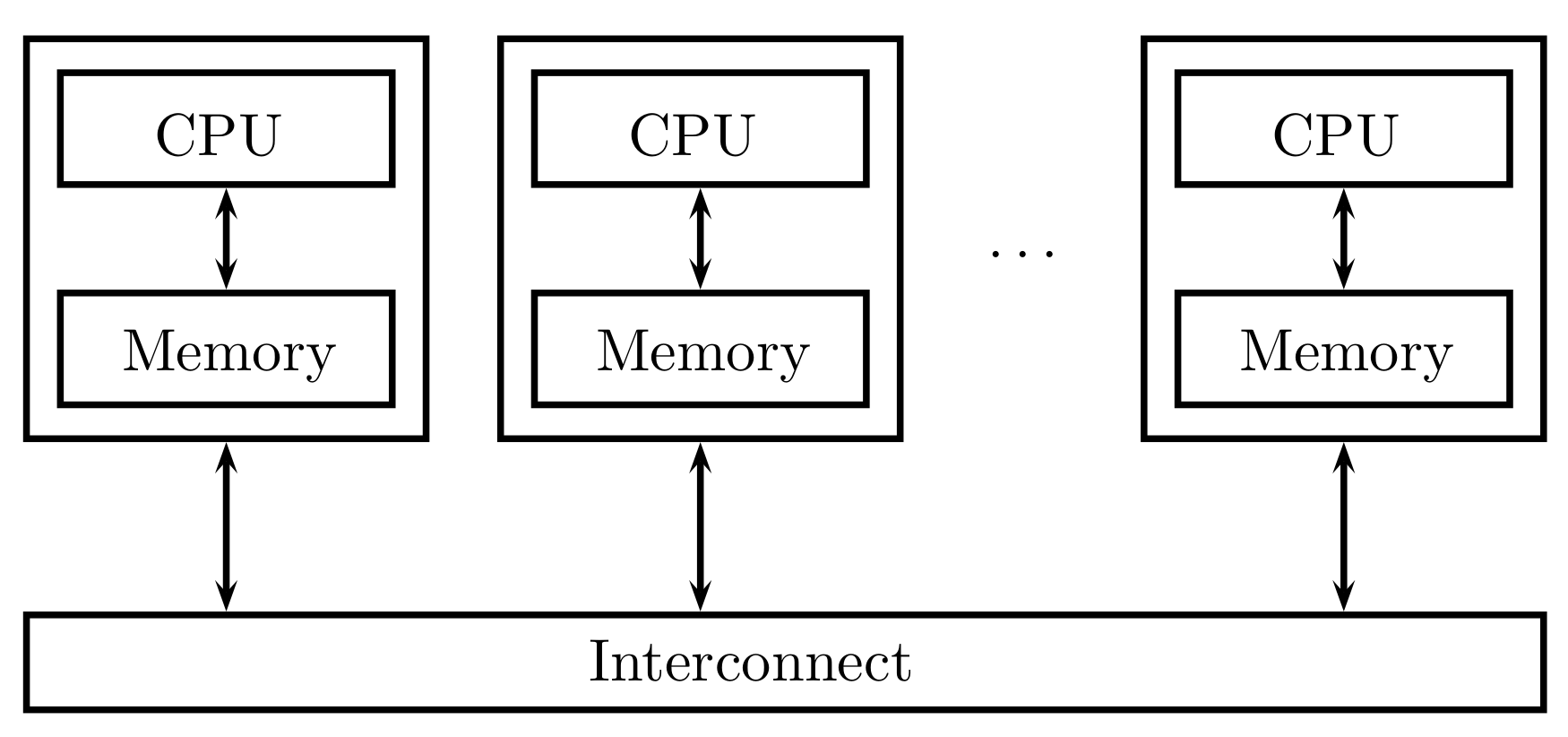
In a distributed memory system (Figure 2), each processor is coupled with its own private memory, and processor-memory pairs communicate over an interconnected network. On distributed memory systems, processors generally communicate explicitly by sending messages or using special functions that provide access to the memory of another processor [24].

3. Description of Virtualization Systems and Process

The strengthening of the cloud computing model has oriented bets on technological resources towards virtualization, and today this methodology has positioned itself as a computational requirement that all kinds of organizations demand for operation, due to the ability to access the information at all times and with the advantage that it allows them to significantly reduce the operating costs in terms of software and hardware resources.

When a cloud computing model becomes extensible, the use of virtualization is increasingly necessary; it is also essential to create new design and integration standards that regulate it. “Virtual infrastructure solutions are ideal for part-to-production environments because they run on industry-standard servers and desktops and are compatible with a wide range of operating systems and application environments, as well as infrastructure and storage” [25].

In the field of computer applications, the infrastructure corresponds to the set of elements that are necessary for the development of an activity [25,26]. In general, two types of infrastructure are identified: hardware (physical) infrastructure and software (logical) infrastructure. The first consists of elements as diverse as air conditioners, sensors, cameras, servers, routers, firewalls, laptops, printers, phones, etc.

The set of logical or software elements ranges from operating systems (Linux, Windows, etc.) to general applications that enable the operation of other specific computer systems of services, such as databases, application servers, or office tools for the suite of applications and computer tools used in the office to optimize, automate, and improve related procedures or tasks.

On the other hand, the term virtualization can be understood as creating through software a virtual version of some technological resource such as a hardware platform, an operating system, a storage device, or another resource network [27].

Nowadays, the consolidation of the cloud computing model has steered towards virtualization as a daily requirement within the technological resources that all kinds of companies require for their operation, permanently accessing and reducing their capital expenditures. The advantages of this model are summarized in three factors: economy, flexibility, and security. A cloud solution can add or remove workstations and servers, and modify their capabilities or configurations almost immediately [28].

A virtualized system includes a new software layer, namely, a virtual machine manager (VMM). The primary function of VMMs is to arbitrate access to resources on the underlying physical host platform so that multiple operating systems (which are VMM guests) can share them. VMM presents each host OS (operating system) with a set of virtual platform interfaces that constitute a virtual machine. Despite once being confined to specialized servers and owners, and high-end mainframe systems, virtualization is now increasingly available. The resulting VMM can support a wider range of legacy and future operating systems while maintaining high performance [29].

The classic benefits of virtualization include better utilization, manageability, and reliability of core framework systems. Multiple users with different operating system requirements can more easily share a virtualized server, operating system updates can be organized on virtual machines to minimize downtime, and the failures of the guest software can be isolated on the virtual machines on which they are produced. While these benefits have traditionally been considered valuable in high-end server systems, recent academic research and new VMM-based emerging products suggest that the benefits of virtualization have greater attractiveness in a wide range of both server and client systems [29].

Virtualization can improve overall system security and reliability by isolating multiple software stacks into self proper virtual machines. Security can be improved because the instructions can be limited to the VM on which they occur, while reliability can be improved because the software failures on one VM do not affect the other VMs [29].

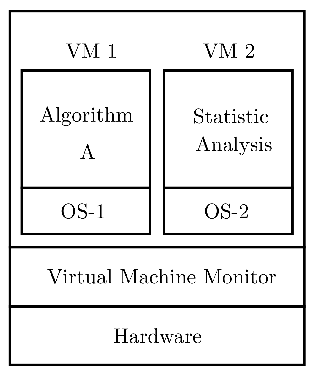
Virtualization allows running the two environments on the same machine, as can be seen in Figure 3, so that these two environments are completely isolated from each other.

In the case of optimization algorithms, the GA algorithm runs on the OS1 operating system and the statistical analysis is executed on the OS2 operating system. Both operating systems run on top of the virtual machine monitor. VMM virtualizes all resources (for example, processors, memory, secondary storage, and networks) and allocates them to the various virtual machines running over VMM [30].

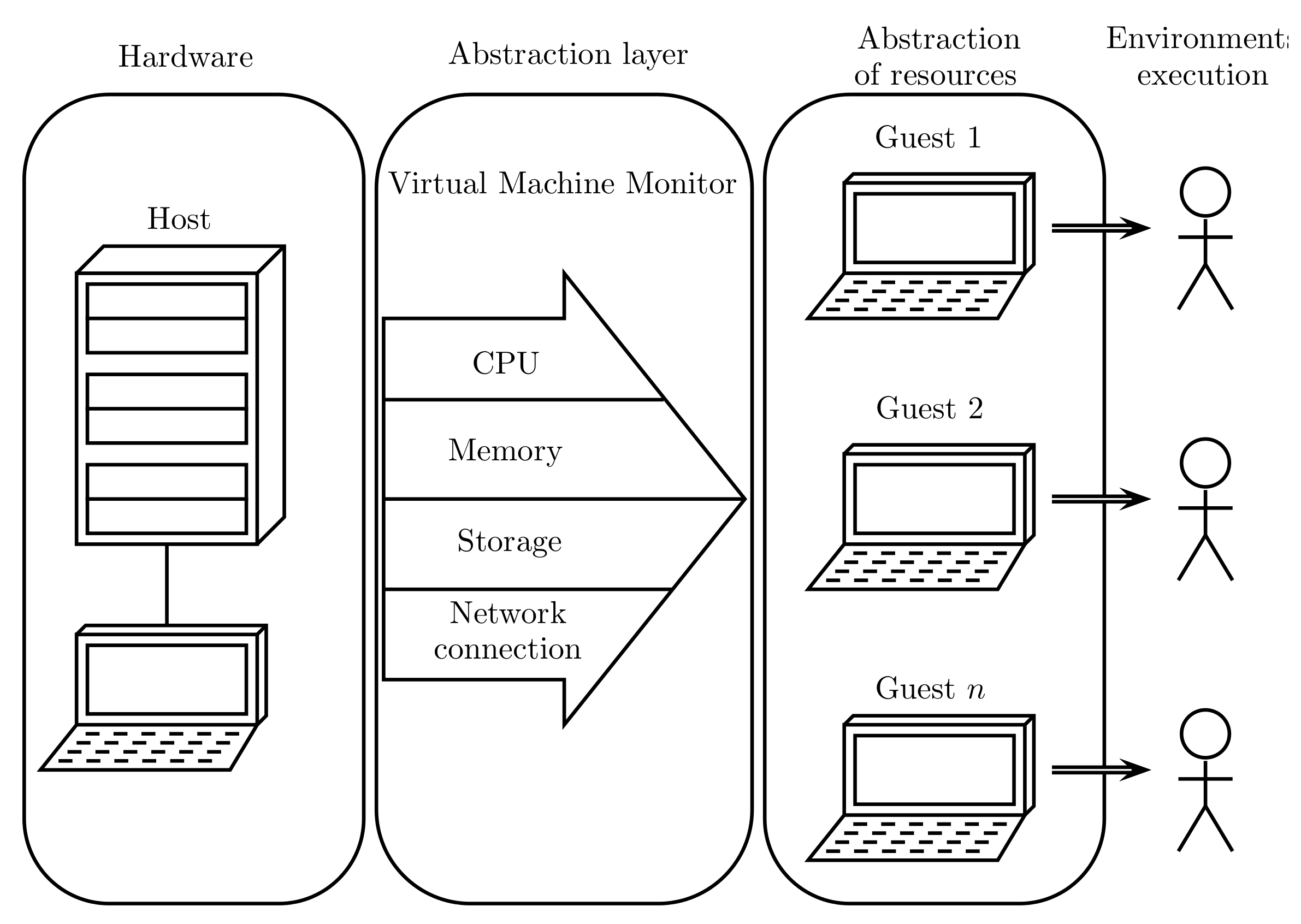
Figure 4 depicts the virtualization process, where the VMM creates an abstraction layer between the host hardware and the virtual machine operating system, appropriately managing its core resources (CPU, memory, storage, and network connections).

4. Virtualized Distributed Processing System Used

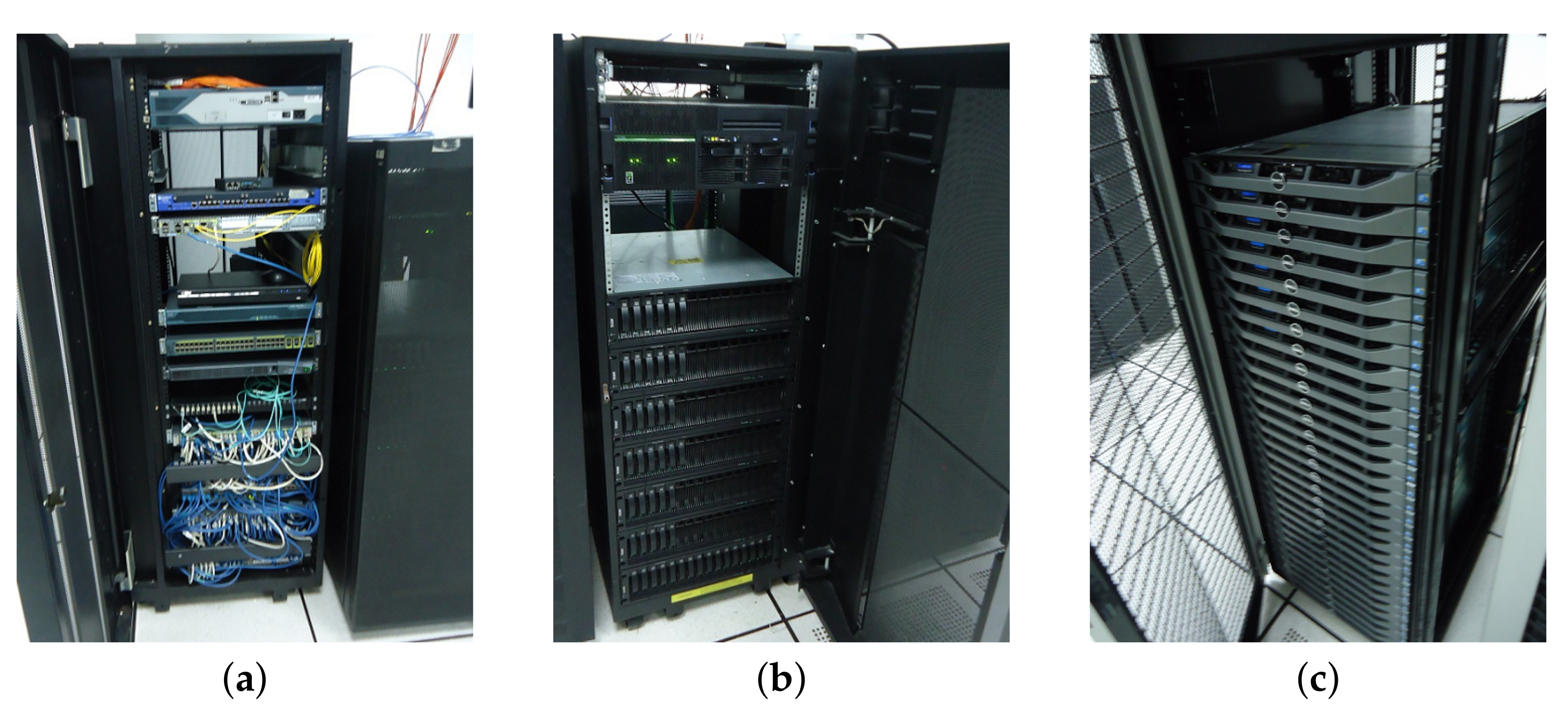
This section describes the virtualized distributed platform for executing bio-inspired optimization algorithms. The computer system consists of network modules, storage, and processing. In Figure 5a is the network module, while Figure 5b shows the storage, and finally, Figure 5c shows the processing system.

This computer system corresponds to the High Performance Computing Center (Centro de Computación de Alto Desempeño—CECAD) of the Universidad Distrital Francisco José de Caldas (UDFJC) which provides a distributed computing service in a virtualized way to the researchers of the UDFJC. Once the resources requested by the researcher are allocated, access to the system can be done remotely.

Infrastructure Used

The characteristics of the infrastructure used are:

• Operating system: Ubuntu Version 18.04.
• RAM memory (GB): 14.5.
• Number of processors: 16.
• Main storage (GB): 80 GB.
• Secondary storage (GB): not used.
• Software used: Octave.

Figure 5c shows the physical appearance of the server used. The features of the R610 Server are:

• 16 processors (Xeon E5570, 2.93 GHz).
• 16 GB DDR3.
• 73 GB hard disk.

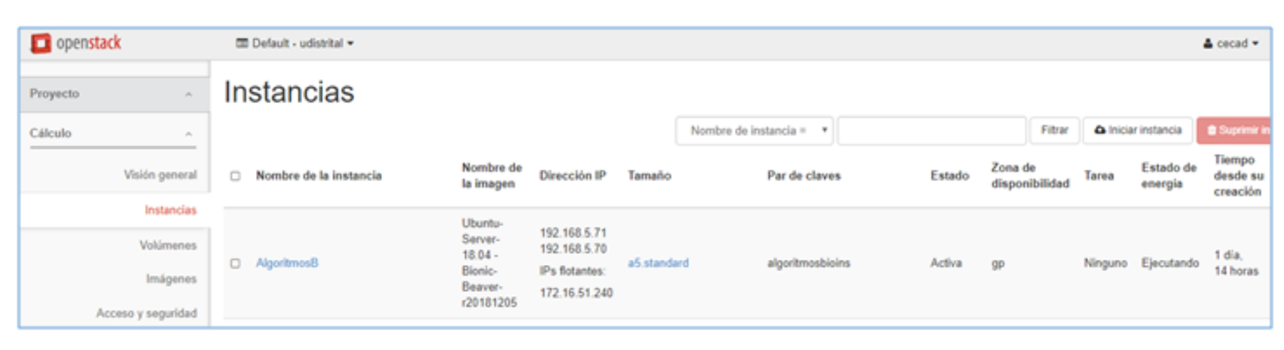
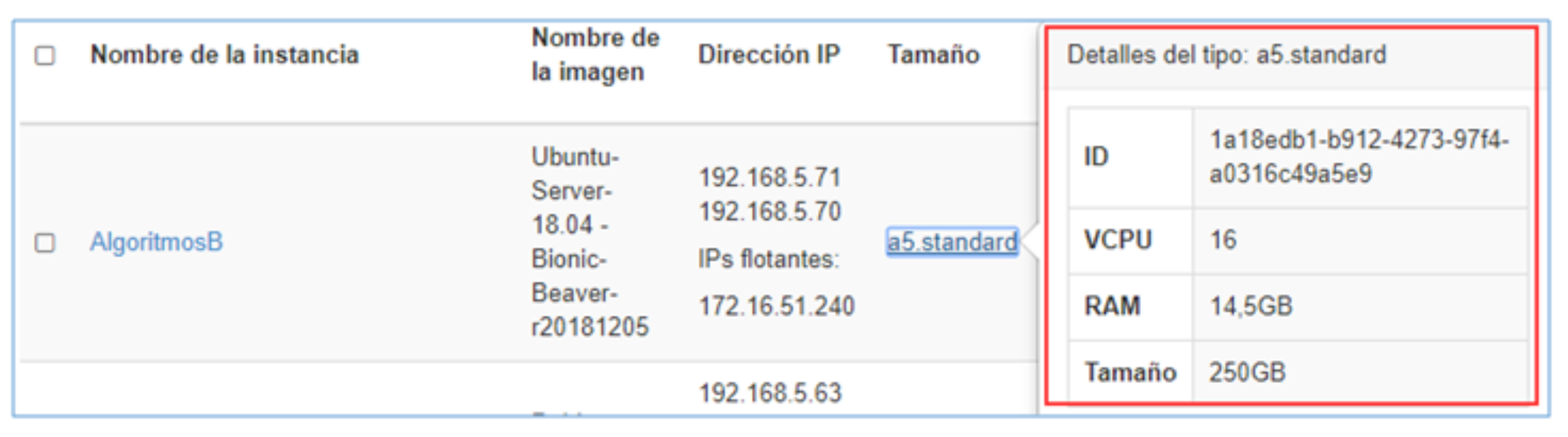
The CECAD private cloud has multiple R610 compute nodes, when using Openstack to provide infrastructure as a service (similar to Amazon EC2); this technology takes one of these servers to deploy the requested instance, in this case the "AlgoritmosB" instance. On the other hand, even though the server storage is apparently limited (73 GB), it has been configured through an architecture that uses the CEPH File System tool, a feature that allows allocating higher storage, in this case of 250 GB, since CEPH is configured to allow nodes to access 100 TB storage from the CECAD SAN. Figure 6 shows the instances using Openstack. The characteristics of the instance used are presented in Figure 7.

5. Bio-Inspirated Optimization Algorithms

The bio-inspired optimization algorithms considered for the testing of the processing system are: genetic algorithms, differential evolution, and optimization based on swarms of particles. The following is the description of these algorithms; then the parameter configuration used is shown.

5.1. Genetic Algorithms

Genetic algorithms (GA) are one of the approaches to stochastic optimization, which is a reference to evolutionary computing algorithms that are based on principles of natural evolution and survival [31]. A GA seeks to improve a population by establishing a point at which the performance function is optimized; thus, simultaneously, multiple candidate solutions are considered [31]. The general steps of a genetic algorithm are as follows:

• Start the population randomly.
• Evaluate the performance of each individual.
• Stochastically select the best individuals.
• Apply the elitism operator.
• Apply the crossover operator.
• Apply the mutation operator.
• If the completion criterion is not met, return to step 2.
• Finish by meeting the stop criterion and establish the final solution.

In the first step an initial population is generated randomly and the fitness function is evaluated for each individual. Then it can use an elitist selection strategy where the best individuals determined by the aptitude assessment move on to the next generation. The next step is to stochastically apply the crossover operator where the parents are selected according to the aptitude value; in this way, individuals who have higher fitness values are selected more frequently. For each pair of parents, the respective crossing is made at random; when not crossing, two children are formed that are copies of the two parents. Subsequently, the operator of the mutation is applied where an element of the individual encoding that has been obtained in the previous step is changed randomly. Finally, the values of the objective function are calculated for the new population and the algorithm is terminated if the stop criterion is met [31,32].

5.2. Differential Evolution Algorithm

The differential evolution (DE) algorithm was initially proposed by Storn and Price [33,34]; this corresponds to an evolutionary computing algorithm where the next population is established considering the subtraction between individuals of the current population using a crossover/recombination operator after the mutation [35]. The main steps of a DE algorithm are as follows:

• Initialize the population in the solution space.
• Apply the subtraction operator.
• Apply the recombination operator.
• Evaluate the performance of each individual.
• Perform the selection process.
• If the completion criterion is not met, return to step 2.
• Finish by meeting the stop criterion and establishing the final solution.

In a first instance, the population is started randomly; then the subtraction operator is applied, followed by the recombination operator; in the next step, the selection process is performed. These processes are performed until the criterion is met.

Taking two randomly chosen individuals $q_1$ and $q_2$ from the population, the subtraction operator incorporates the difference between these individuals into a third individual $q_3$ in such a way that it has a new $p_i$ individual which corresponds to:

$$p_i=q_1+\mu (q_2-q_3)$$

(1)

Using the mutation constant $\mu >0$, the subtraction between individuals is set. After the mutation, a recombination operation is performed on each $q_i$ individual to generate a $u_i$ individual which is constructed by mixing the $p_i$ and $q_i$ components. This is what a random number is used for $P\in [0,1]$ having the follow equation:

$$u_i=\left\{\begin{array}{cc}{p}_i\left(l\right),\hfill & \mathrm{if} \mathrm{rand}<P;\hfill \\ q_i\left(l\right),\hfill & \mathrm{otherwise}.\hfill \end{array}\right.$$

(2)

If an improvement of the objective function is achieved with the intermediate individual $u_i$, this replaces the individual $q_i$; otherwise, it remains $q_i$ in the next generation.

5.3. Particle Swarm Optimization Algorithm

The concept of swarm-based optimization was proposed by James Kennedy and Russell Eberhart based on the social behavior of bird flocks [6]. In general, the steps involved in the PSO (particle swarm optimization) algorithm are as follows:

• Initialize the swarm in the solution space.
• Evaluate the performance of each individual.
• Find the best individual and collective performances.
• Calculate the speed and position of each individual.
• Move each individual to the new position.
• If the completion criterion is not met, return to step 2.
• Finish by meeting the stop criterion and establishing the final solution.

As it is appreciated, in a first instance the swarm is initialized in the solution space; then the performance of each individual is evaluated by finding the best individual and collective performances; with these values the speed of each particle is calculated. That is used to determine the displacement of each individual to the new position. The above processes are carried out until a completion criterion. The following expression is used to establish the position of each individual:

$${\overrightarrow{x}}_i[n+1]={\overrightarrow{x}}_i\left[n\right]+{\overrightarrow{v}}_i[n+1]$$

(3)

For the calculation of the speed there are different alternatives, one of the most representative ones being the one which incorporates an inertia factor described by the following equation:

$${\overrightarrow{v}}_i[n+1]=w{\overrightarrow{v}}_i\left[n\right]+{\alpha }_p\left[{\beta }_{pi}({\overrightarrow{x}}_{p_i}-{\overrightarrow{x}}_i\left[n\right])\right]+{\alpha }_g\left[{\beta }_{gi}({\overrightarrow{x}}_g-{\overrightarrow{x}}_i\left[n\right])\right]$$

(4)

In the above equations, ${\overrightarrow{v}}_i$ and ${\overrightarrow{x}}_i$ correspond to the velocity and position of the individual i-th. On the other hand, ${\overrightarrow{x}}_{p_i}$ is the best position found by the i-th individual, and ${\overrightarrow{x}}_g$ is the best position found by the swarm. Additionally, ${\beta }_{pi}$ and ${\beta }_{gi}$ are random numbers in the range $[0,1]$. Finally, w is an inertia value, ${\alpha }_p$ acceleration constant of the social part and ${\alpha }_g$ acceleration of the cognitive part.

6. Experiments Configuration

The configuration of the algorithms is done considering two representative cases, which are executed on eight test functions with and without virtualization. With these experiments we sought to show that the virtualization scheme allows reducing the execution times of the algorithms without altering their performances.

6.1. Configuration for Genetic Algorithms

Two recommended standard configurations are used for the case considered. The first configuration uses 50 individuals with mutation probability of $0.001$ and crossover probability of 0.6 [36]. The second configuration has 30 individuals, mutation probability of $0.01$, and probability associated to the genes exchanged between individuals equal to $0.9$ [37].

Table 1. Parameters configurations for the genetic algorithm.

Configuration	Parameters
	Population	Mutation (Prob.)	Crossover (Prob.)
AG-C1	50	0.001	0.6
AG-C2	30	0.01	0.9

summarizes the deployed configurations.

6.2. Configuration for Differential Evolution

The method of differential evolution starts from a randomly initialized population, with which the following population establishes itself, considering the difference between individuals of that population. Two configurations of the differential evolution algorithm were used for this algorithm, considering the recommendations proposed by [38].

The first configuration has 40 members, probability of crossing equal to $0.9784$, and the step size of $0.6876$; for the second configuration, taking into account the rule given by Price and Storn [33], the number of members is 20, the probability of crossing is 1 since the high values guarantee the appropriate contour conditions for the evolution algorithm [34], and the step size is $0.85$. The summary of the configurations is presented in

Table 2. Parameters’ configurations for the differential evolution algorithm.

Configuration	Parameters
	Population	Crossover (Prob.)	Step Size
DE-C1	48	0.9784	0.6876
DE-C2	20	1	0.85

.

6.3. Particle Swarm Optimization Configuration

For PSO, the two configurations proposed by [39] are used for the PSO algorithm with inertia factor. Parameter selection is based on an analysis of the dynamic behavior of the swarm. Both cases use 30 particles;

Table 3. Parameter configuration for particle swarm optimization.

Configuration	Parameters
	$\mathit{w}$	${\mathit{\alpha }}_{\mathit{p}}$	${\mathit{\alpha }}_{\mathit{g}}$
PSO-C1	0.600	1.7	1.7
PSO-C2	0.729	1.494	1.494

shows the selected configurations.

7. Tests Functions

Ideally, the test functions chosen to evaluate an optimization algorithm should contain features similar to the real-world problem. However, specialized literature is characterized by the use of artificial functions to perform tests on these optimization algorithms.

The multi-dimensional test functions can be seen in

Table 4. Generalized test functions used.

Name	Dim	Limits	Equation
Spherical	D	${[-100,100]}^D$	$f_1\left(\overrightarrow{x}\right)={\displaystyle \sum _{i=1}^D}{x}_i^2$
Levy	D	${[-10,10]}^D$	$f_2\left(\overrightarrow{x}\right)={sin}^2\left(\pi w_1\right)+{\displaystyle \sum _{i=1}^{D-1}}{(w_i-1)}^2[1+10{sin}^2(\pi w_i+1)]+{(w_D-1)}^2[1+{sin}^2\left(2\pi w_D\right)]$, where, $w_i=1+\frac{x_i-1}{4}$
Styblinski Tang	D	${[-5.12,5.12]}^D$	$f_3\left(\overrightarrow{x}\right)=\frac{1}{2}{\displaystyle \sum _{i=1}^D}\left(x_i^4-16x_i^2+5x_i\right)$
Rosenbrock Rotate	D	${[-30,30]}^D$	$f_4\left(\overrightarrow{x}\right)={\displaystyle \sum _{i=1}^{D-1}}{\left[100{(x_{i+1}+x_i^2)}^2+{(x_i+1)}^2\right]}^2$
Griewank	D	${[-50,50]}^D$	$f_5\left(\overrightarrow{x}\right)=1+\frac{1}{4000}{\displaystyle \sum _{i=1}^D}{x}_i^2-{\displaystyle \prod _{i=1}^D}cos\left(\frac{x_i}{\sqrt{i}}\right)$
Rastrigin	D	${[-5.12,5.12]}^D$	$f_6\left(\overrightarrow{x}\right)={\displaystyle \sum _{i=1}^D}\left(x_i^2-10cos\left(2\pi x_i\right)+10\right)$
Schaffer	D	${[-30,30]}^D$	$f_7\left(\overrightarrow{x}\right)={\displaystyle \sum _{i=1}^{D-1}}{(x_i^2+x_{i+1}^2)}^{0.25}\left[{sin}^2\left(50{(x_i^2+x_{i+1}^2)}^{0.1}\right)+1\right]$
Ackley	D	${[-30,30]}^D$	$f_8\left(\overrightarrow{x}\right)=e+20-20exp\left(-0.2\sqrt{\frac{1}{D}{\displaystyle \sum _{i=1}^D}{x}_i^D}\right)$$-exp\left(\frac{1}{D}{\displaystyle \sum _{i=1}^D}cos\left(2\pi x_i\right)\right)$

; the selection was made considering the reports [40,41,42,43], wherein they are used for testing with bio-inspired algorithms. The characteristics of the test functions can be seen in

Table 5. Features of the test functions used.

Name	Dim	Multi-Modal	Optimal Point	Limits	Optimal Value
Spherical	D	No	${\left(0.0\right)}^D$	${[-100,100]}^D$	0
Levy	D	Yes	${\left(1.0\right)}^D$	${[-10,10]}^D$	0
Styblinski Tang	D	Yes	${(-2.903534)}^D$	${[-5.12,5.12]}^D$	$-39.16599D$
Rosenbrock Rotate	D	Yes	${(-1.0)}^D$	${[-30,30]}^D$	0
Griewank	D	Yes	${\left(0.0\right)}^D$	${[-50,50]}^D$	0
Rastrigin	D	Yes	${\left(0.0\right)}^D$	${[-5.12,5.12]}^D$	0
Schaffer	D	Yes	${\left(0.0\right)}^D$	${[-30,30]}^D$	0
Ackley	D	Yes	${\left(0.0\right)}^D$	${[-30,30]}^D$	0

. This table shows that the functions employed have different limits of the search space.

As noted in Table 5, the test functions $f_2$, $f_3$, and $f_4$ have the minimum localized value at a non-zero point, while for all other test functions the global minimum is located at zero.

8. Experimental Results

This section compares the performances of the selected bio-inspired algorithms with and without the virtualization scheme. The results are first reviewed considering the value obtained from the target function, and then the results obtained from the execution time (run-time) are analyzed.

In these results M2 corresponds to the distributed processing scheme, while M1 refers to the dedicated PC (personal computer) with the following characteristics.

• Operating System: Windows 8.
• RAM Memory (GB): 6.
• Processor: i5 2.60 GHz.
• Main storage (GB): 680 GB.
• Software used: Octave.

In both cases, the algorithms and data collection were performed in the free Octave software. Each configuration ran 50 times for each test function (taking 10 dimensions).

In order to identify the results, the first part of the respective tag refers to the class of algorithm AG, DE, or PSO; then the type of configuration C1 or C2 is indicated; finally, the machine is M1 or M2, with which the algorithm was executed.

Here are used different source files for experiments; for the implementation of GA the source from GitHub posted by user "shenbennwdsl" in [44] was used; in the case of DE, the files developed by Rainer Storn, Ken Price, Arnold Neumaier, and Jim Van Zandt posted in [45]; for PSO the source file developed by Matthew P. Kelly downloaded from [46]; for test functions, the archives developed by Brian Birge from [47] were used; and Sonja Surjanovic and Derek Bingham posted in [48]. Finally, all archives used in this work to implement the experiments and present the results can be downloaded from GitHub in [49].

8.1. GA Algorithm Results

Table 6. Statistical results for the value of the objective function using GA.

$f_1$	GA-C1-M1	GA-C2-M1	GA-C1-M2	GA-C2-M2
Max	803.1	851.1	693.48	878.87
Min	110.12	231.66	96.881	198.67
Average	396.34	512.71	363.63	524.55
STD	164.16	145.59	165.86	165.07
$f_2$	GA-C1-M1	GA-C2-M1	GA-C1-M2	GA-C2-M2
Max	4.0682	2.8756	4.1886	2.9012
Min	0.43532	0.73858	0.50167	0.49925
Average	2.0062	1.6742	1.7204	1.6712
STD	1.094	0.43556	0.91603	0.49293
$f_3$	GA-C1-M1	GA-C2-M1	GA-C1-M2	GA-C2-M2
Max	−361.86	−369.18	−360.01	−366.04
Min	−385.82	−390.21	−389.06	−385.25
Average	−376.93	−378.57	−377.46	−378.18
STD	5.3254	4.3697	5.5337	4.2567
$f_4$	GA-C1-M1	GA-C2-M1	GA-C1-M2	GA-C2-M2
Max	$7.484\times {10}^5$	$2.6675\times {10}^5$	$6.5106\times {10}^5$	$2.7881\times {10}^5$
Min	11809	22674	10592	14904
Average	$2.1762\times {10}^5$	$1.2786\times {10}^5$	$2.032\times {10}^5$	$1.1931\times {10}^5$
STD	$1.81\times {10}^5$	61355	$1.6132\times {10}^5$	59792
$f_5$	GA-C1-M1	GA-C2-M1	GA-C1-M2	GA-C2-M2
Max	1.0079	0.90574	1.0422	0.95218
Min	0.13795	0.51898	0.13518	0.4226
Average	0.62559	0.72619	0.64354	0.72477
STD	0.29169	0.10053	0.27751	0.11398
$f_6$	GA-C1-M1	GA-C2-M1	GA-C1-M2	GA-C2-M2
Max	26.967	22.369	26.161	23.734
Min	9.0212	11.351	6.8412	7.9241
Average	18.404	17.323	16.87	17.45
STD	4.2545	2.6509	4.1317	3.2635
$f_7$	GA-C1-M1	GA-C2-M1	GA-C1-M2	GA-C2-M2
Max	15.554	15.825	15.913	16.091
Min	5.81	9.5476	6.1036	9.749
Average	9.7471	13.107	9.4184	13.142
STD	2.1818	1.3576	2.1384	1.3547
$f_8$	GA-C1-M1	GA-C2-M1	GA-C1-M2	GA-C2-M2
Max	3.4624	5.2211	3.8739	5.3901
Min	0.88282	3.3081	1.2655	3.0742
Average	2.4774	4.2857	2.7235	4.253
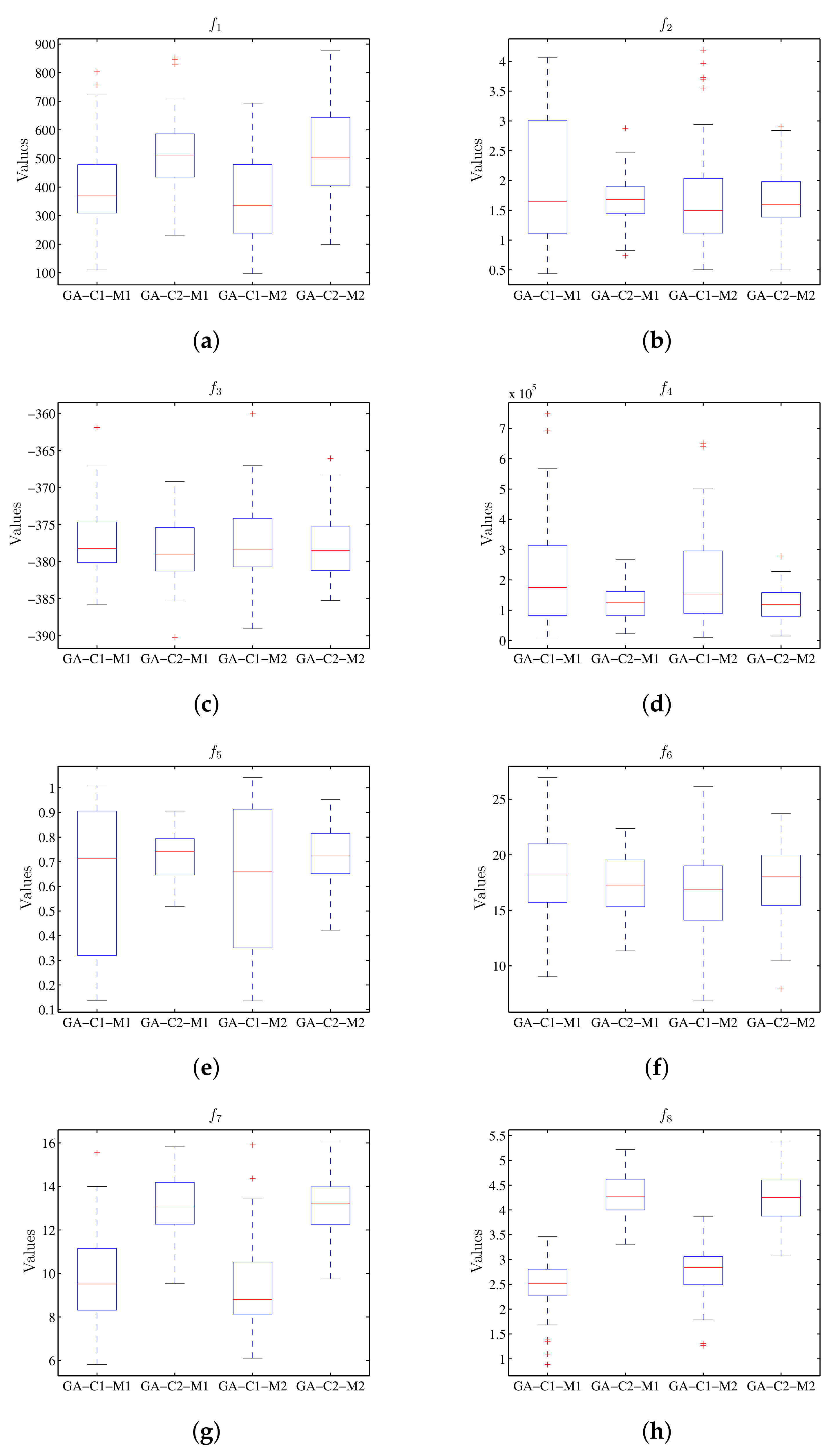
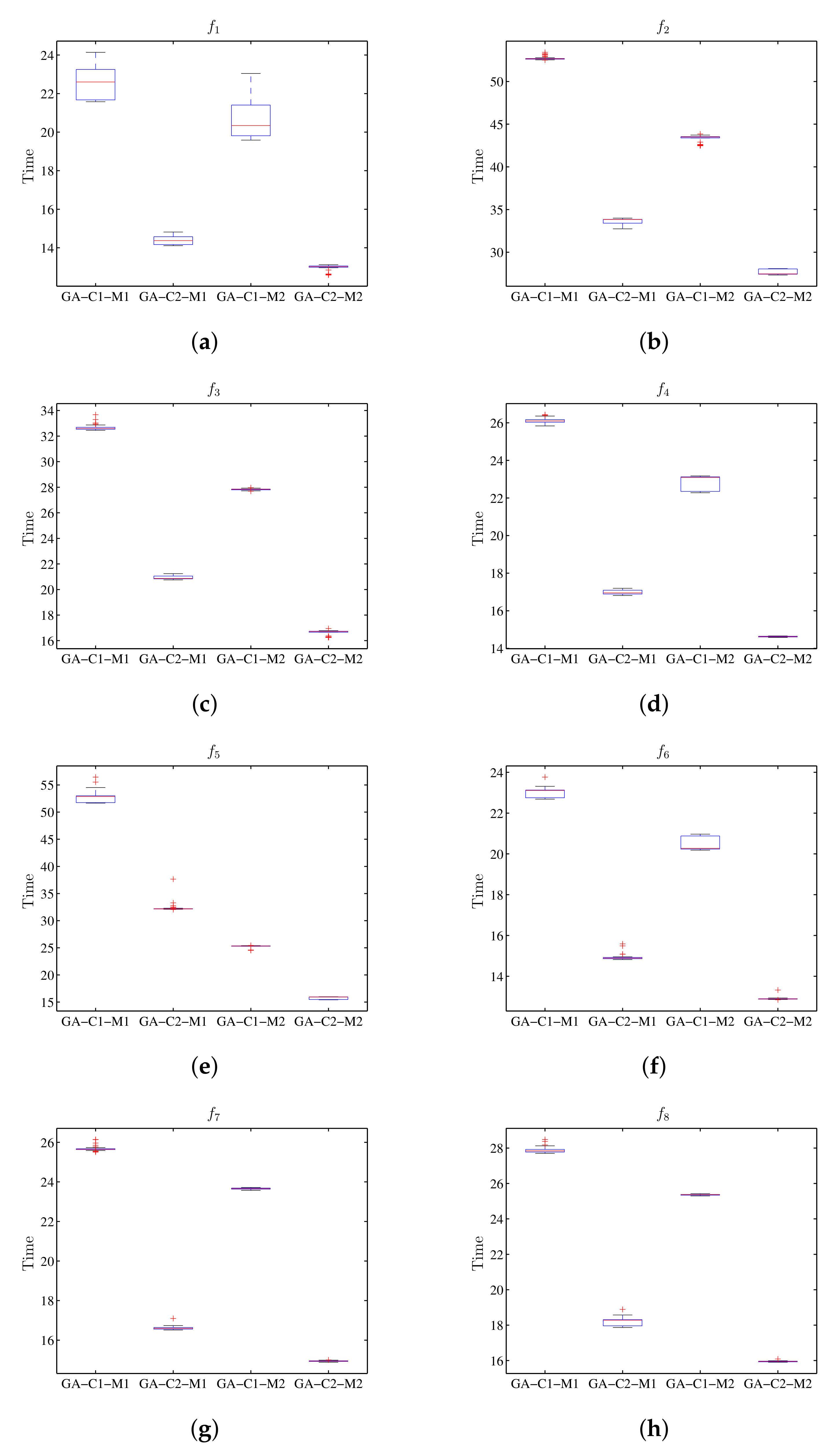
STD	0.5349	0.44425	0.55014	0.53566

shows the results when performing the execution of the genetic algorithm for the value of the target function, and

Table 7. Statistical results for the execution time (run-time), using GA.

$f_1$	GA-C1-M1	GA-C2-M1	GA-C1-M2	GA-C2-M2
Max	24.144	14.818	23.045	13.121
Min	21.58	14.109	19.585	12.583
Average	22.567	14.376	20.548	12.98
STD	0.83158	0.21588	0.78465	0.14111
$f_2$	GA-C1-M1	GA-C2-M1	GA-C1-M2	GA-C2-M2
Max	53.419	33.995	43.846	28.084
Min	52.5	32.746	42.469	27.325
Average	52.705	33.576	43.305	27.68
STD	0.19373	0.45674	0.40224	0.29811
$f_3$	GA-C1-M1	GA-C2-M1	GA-C1-M2	GA-C2-M2
Max	33.675	21.241	27.961	16.951
Min	32.444	20.753	27.693	16.249
Average	32.656	20.933	27.829	16.625
STD	0.2189	0.12987	0.051181	0.19769
$f_4$	GA-C1-M1	GA-C2-M1	GA-C1-M2	GA-C2-M2
Max	26.432	17.195	23.177	14.662
Min	25.832	16.809	22.28	14.579
Average	26.12	16.988	22.806	14.625
STD	0.12577	0.10671	0.3793	0.021441
$f_5$	GA-C1-M1	GA-C2-M1	GA-C1-M2	GA-C2-M2
Max	56.463	37.643	25.431	15.981
Min	51.667	32.043	24.527	15.403
Average	52.609	32.336	25.207	15.777
STD	0.98871	0.79033	0.28878	0.2308
$f_6$	GA-C1-M1	GA-C2-M1	GA-C1-M2	GA-C2-M2
Max	23.767	15.585	20.968	13.325
Min	22.686	14.818	20.182	12.843
Average	23.014	14.918	20.424	12.898
STD	0.22193	0.13802	0.30039	0.063915
$f_7$	GA-C1-M1	GA-C2-M1	GA-C1-M2	GA-C2-M2
Max	26.147	17.097	23.718	15.003
Min	25.505	16.514	23.571	14.883
Average	25.675	16.608	23.661	14.943
STD	0.1198	0.087461	0.031198	0.023558
$f_8$	GA-C1-M1	GA-C2-M1	GA-C1-M2	GA-C2-M2
Max	28.488	18.888	25.426	16.091
Min	27.7	17.862	25.294	15.904
Average	27.885	18.179	25.365	15.948
STD	0.15947	0.21193	0.032987	0.029009

shows the results for the run-time. Graphically, the results obtained for the values of the target function can be seen in a diagram of stems and sheets in Figure 8 and Figure 9 for run-time. In Figure 8 the configurations associated to M1 and M2 present similar results for the objective functions; meanwhile, in Figure 9 in all cases the processing time associated with machine M2 is less that than of M1.

8.2. DE Algorithm Results

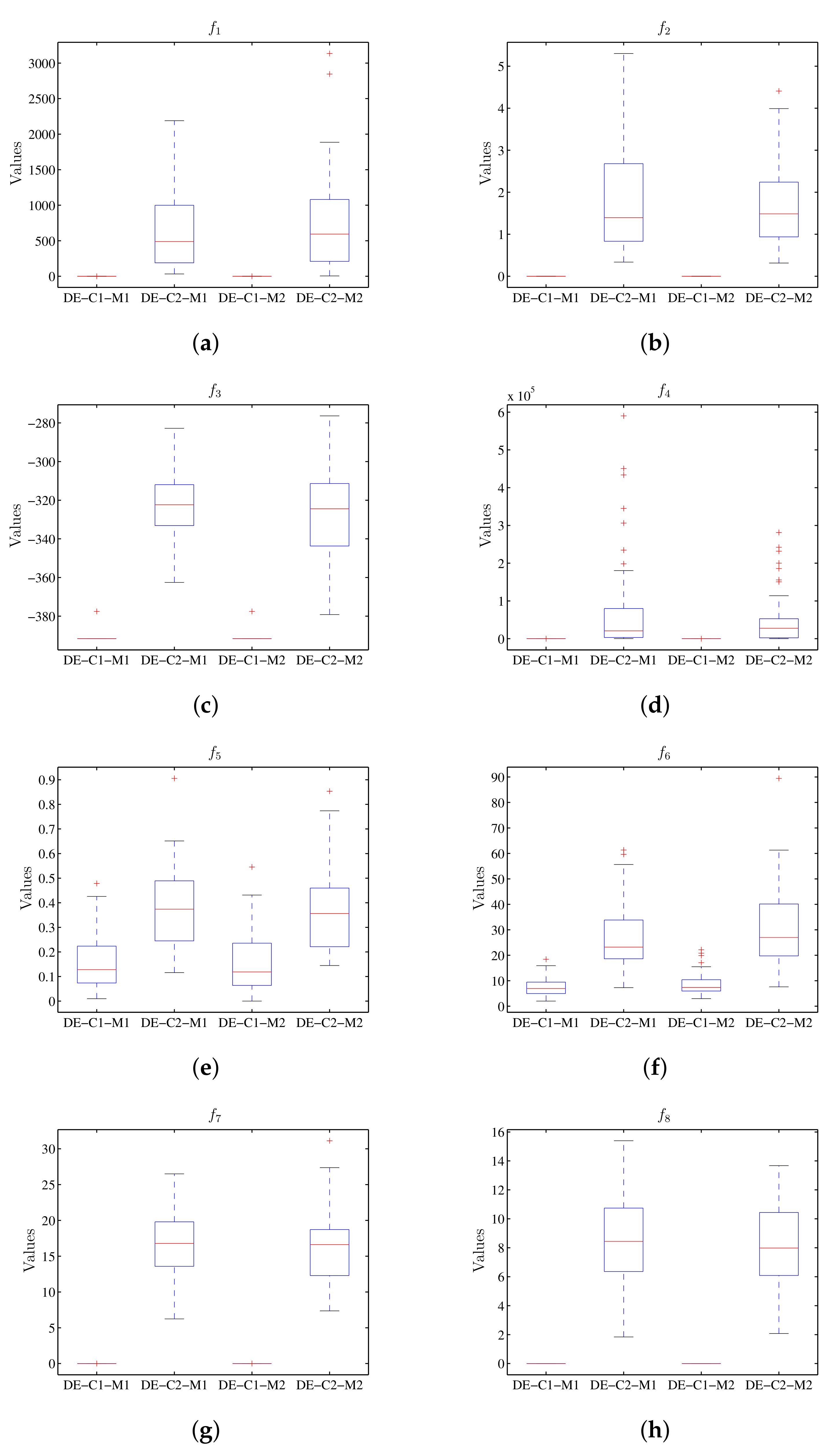
The execution of the differential evolution algorithm in

Table 8. Statistical results for the value of the objective function using DE.

$f_1$	DE-C1-M1	DE-C2-M1	DE-C1-M2	DE-C2-M2
Max	$3.0967\times {10}^{-36}$	2189.2	$6.7457\times {10}^{-36}$	3135.8
Min	$1.1902\times {10}^{-38}$	33.487	$3.852\times {10}^{-39}$	5.1453
Average	$4.4506\times {10}^{-37}$	637.3	$5.6028\times {10}^{-37}$	738.21
STD	$6.8787\times {10}^{-37}$	508.86	$1.1785\times {10}^{-36}$	680.65
$f_2$	DE-C1-M1	DE-C2-M1	DE-C1-M2	DE-C2-M2
Max	$1.4997\times {10}^{-32}$	5.303	$1.4998\times {10}^{-32}$	4.4089
Min	$1.4997\times {10}^{-32}$	0.33872	$1.4998\times {10}^{-32}$	0.31488
Average	$1.4997\times {10}^{-32}$	1.8351	$1.4998\times {10}^{-32}$	1.6916
STD	$2.7647\times {10}^{-48}$	1.2641	$8.2941\times {10}^{-48}$	0.99901
$f_3$	DE-C1-M1	DE-C2-M1	DE-C1-M2	DE-C2-M2
Max	−377.52	−282.82	−377.52	−276.36
Min	−391.66	−362.53	−391.66	−379.17
Average	−390.53	−322.34	−391.1	−324.16
STD	3.8741	17.26	2.7983	24.568
$f_4$	DE-C1-M1	DE-C2-M1	DE-C1-M2	DE-C2-M2
Max	3.9866	$5.9015\times {10}^5$	3.9866	$2.8148\times {10}^5$
Min	0	221.75	$1.0452\times {10}^{-29}$	85.7
Average	0.31893	79546	0.079732	51649
STD	1.0925	$1.322\times {10}^5$	0.56379	71056
$f_5$	DE-C1-M1	DE-C2-M1	DE-C1-M2	DE-C2-M2
Max	0.47846	0.90603	0.54541	0.8534
Min	0.0098573	0.11603	0	0.14461
Average	0.17114	0.37272	0.15415	0.36911
STD	0.12517	0.16561	0.12216	0.17738
$f_6$	DE-C1-M1	DE-C2-M1	DE-C1-M2	DE-C2-M2
Max	18.436	61.339	22.189	89.495
Min	1.9899	7.284	2.9849	7.5864
Average	7.6318	26.926	8.9962	30.295
STD	3.5215	12.042	4.4606	15.282
$f_7$	DE-C1-M1	DE-C2-M1	DE-C1-M2	DE-C2-M2
Max	0.00025313	26.502	0.00023235	31.125
Min	$4.4825\times {10}^{-6}$	6.2426	$2.782\times {10}^{-6}$	7.3592
Average	$3.1826\times {10}^{-5}$	16.616	$4.163\times {10}^{-5}$	16.469
STD	$3.8948\times {10}^{-5}$	4.8337	$4.6877\times {10}^{-5}$	4.8209
$f_8$	DE-C1-M1	DE-C2-M1	DE-C1-M2	DE-C2-M2
Max	$3.1086\times {10}^{-15}$	15.395	$3.1086\times {10}^{-15}$	13.672
Min	$3.1086\times {10}^{-15}$	1.8371	$3.1086\times {10}^{-15}$	2.0741
Average	$3.1086\times {10}^{-15}$	8.5284	$3.1086\times {10}^{-15}$	7.9863
STD	0	2.8974	0	3.0219

shows the summary of the statistical results for the value of the target function, while

Table 9. Statistical results for the execution time using DE.

$f_1$	DE-C1-M1	DE-C2-M1	DE-C1-M2	DE-C2-M2
Max	16.266	7.5975	13.654	5.8533
Min	15.431	6.7975	11.854	5.2711
Average	15.772	7.038	12.245	5.343
STD	0.18457	0.14197	0.38329	0.078526
$f_2$	DE-C1-M1	DE-C2-M1	DE-C1-M2	DE-C2-M2
Max	57.416	23.251	34.549	15.018
Min	48.193	20.763	33.857	14.653
Average	49.606	21.304	34.325	14.75
STD	1.8648	0.58789	0.20726	0.049601
$f_3$	DE-C1-M1	DE-C2-M1	DE-C1-M2	DE-C2-M2
Max	27.869	12.068	18.801	8.2856
Min	26.586	11.451	18.492	8.1547
Average	27.24	11.765	18.633	8.2207
STD	0.23964	0.13481	0.068874	0.031299
$f_4$	DE-C1-M1	DE-C2-M1	DE-C1-M2	DE-C2-M2
Max	20.083	9.6074	15.165	6.5915
Min	18.842	8.8058	14.626	6.4609
Average	19.604	8.9937	14.947	6.5287
STD	0.22143	0.13871	0.17267	0.032574
$f_5$	DE-C1-M1	DE-C2-M1	DE-C1-M2	DE-C2-M2
Max	28.155	12.564	21.205	7.9327
Min	21.609	9.5708	16.104	7.3504
Average	23.728	10.065	16.841	7.4283
STD	1.3008	0.57603	0.82097	0.080032
$f_6$	DE-C1-M1	DE-C2-M1	DE-C1-M2	DE-C2-M2
Max	20.134	10.592	15.865	7.8398
Min	16.432	7.5325	12.441	5.7978
Average	17.298	8.1412	12.988	6.0956
STD	0.59429	0.8543	0.66904	0.54322
$f_7$	DE-C1-M1	DE-C2-M1	DE-C1-M2	DE-C2-M2
Max	20.159	11.566	15.484	8.8737
Min	19.054	8.5482	15.042	6.7808
Average	19.593	9.0394	15.397	7.171
STD	0.33105	0.70994	0.088293	0.57938
$f_8$	DE-C1-M1	DE-C2-M1	DE-C1-M2	DE-C2-M2
Max	23.642	12.882	17.531	7.8927
Min	22.782	9.805	17.011	7.4364
Average	23.23	10.159	17.413	7.5943
STD	0.19133	0.44989	0.13786	0.069855

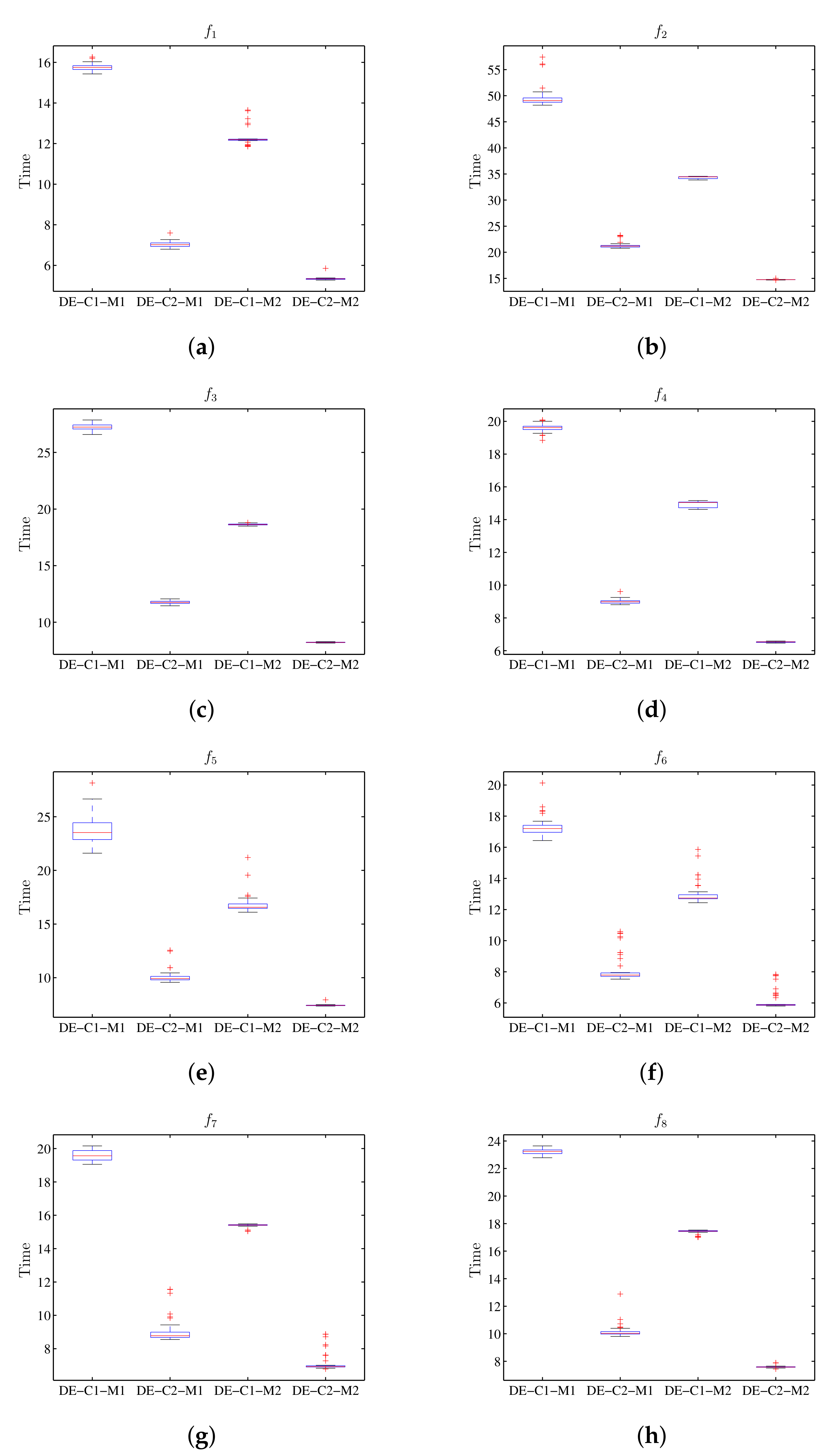
has the run-time. The graphical presentation of the results obtained is shown in Figure 10; the diagrams of stems and sheets for the value of the target function are also shown. Figure 11 provides the diagrams of stems and sheets for the run-time. The results of Figure 10 show that configuration C1 of the DE algorithm executed in machine M1 has similar results to those obtained in machine M2 for the value of objective function; the same happens using configuration C2 when executed in M1 and M2. Meanwhile, considering the run-time, Figure 11 shows that when executing the configuration C1 in machine M2, less run-time is observed compared to the same execution using machine M1; for configuration C2 there is also less run-time when using M2.

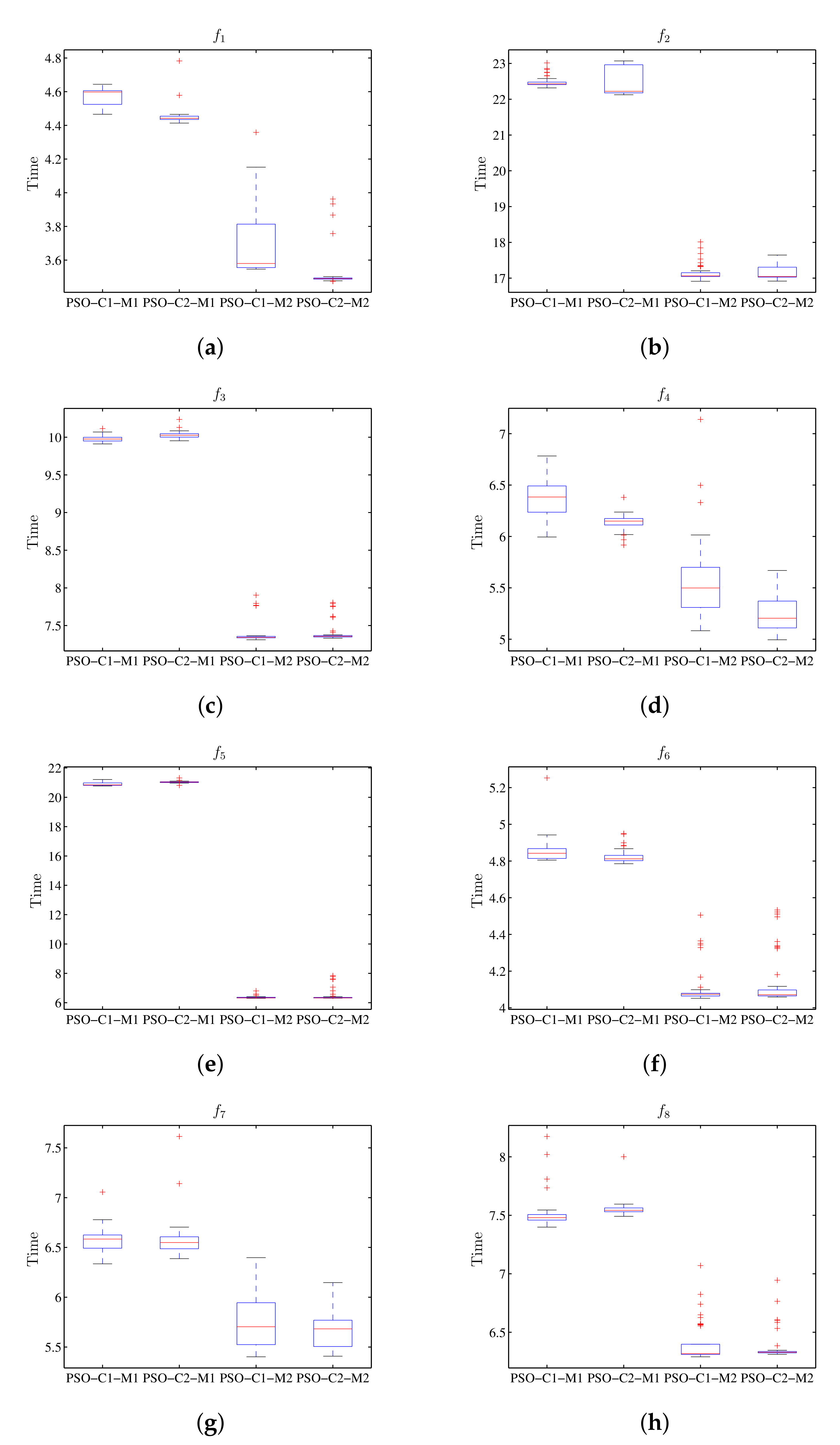
8.3. PSO Algorithm Results

Table 10. Statistical results for the value of the objective function using PSO.

$f_1$	PSO-C1-M1	PSO-C2-M1	PSO-C1-M2	PSO-C2-M2
Max	$3.4482\times {10}^{-128}$	$3.4909\times {10}^{-92}$	$2.0141\times {10}^{-127}$	$8.0804\times {10}^{-92}$
Min	$4.0135\times {10}^{-136}$	$1.1576\times {10}^{-99}$	$5.7269\times {10}^{-136}$	$4.0316\times {10}^{-100}$
Average	$2.3691\times {10}^{-129}$	$1.0474\times {10}^{-93}$	$7.6416\times {10}^{-129}$	$2.6889\times {10}^{-93}$
STD	$6.8822\times {10}^{-129}$	$5.0295\times {10}^{-93}$	$3.1639\times {10}^{-128}$	$1.1853\times {10}^{-92}$
$f_2$	PSO-C1-M1	PSO-C2-M1	PSO-C1-M2	PSO-C2-M2
Max	0.45432	1.1605	3.3738	0.45432
Min	$1.4997\times {10}^{-32}$	$1.4997\times {10}^{-32}$	$1.4998\times {10}^{-32}$	$1.4998\times {10}^{-32}$
Average	0.036212	0.044963	0.18755	0.023545
STD	0.11155	0.18929	0.60021	0.091378
$f_3$	PSO-C1-M1	PSO-C2-M1	PSO-C1-M2	PSO-C2-M2
Max	−335.11	−335.11	−320.98	−335.11
Min	−391.66	−391.66	−391.66	−391.66
Average	−363.95	−371.02	−365.37	−371.02
STD	17.127	15.698	17.608	14.898
$f_4$	PSO-C1-M1	PSO-C2-M1	PSO-C1-M2	PSO-C2-M2
Max	7.7008	150.43	125.9	97.773
Min	0.001011	0.00075109	$9.3565\times {10}^{-5}$	$8.2241\times {10}^{-5}$
Average	2.3245	5.2944	4.0551	5.0642
STD	2.2494	21.749	17.666	17.601
$f_5$	PSO-C1-M1	PSO-C2-M1	PSO-C1-M2	PSO-C2-M2
Max	0.2658	0.17454	0.22621	0.18699
Min	0.017236	0.007396	0	0.01969
Average	0.082166	0.067271	0.073552	0.081583
STD	0.045771	0.032932	0.046	0.036983
$f_6$	PSO-C1-M1	PSO-C2-M1	PSO-C1-M2	PSO-C2-M2
Max	13.929	12.934	15.919	15.919
Min	0	1.9899	0	0.99496
Average	7.1836	6.507	7.9995	6.6861
STD	3.1674	2.942	3.5275	3.5107
$f_7$	PSO-C1-M1	PSO-C2-M1	PSO-C1-M2	PSO-C2-M2
Max	4.6907	5.0196	5.8513	5.4093
Min	0.010729	$5.7752\times {10}^{-23}$	0.010729	$1.0224\times {10}^{-23}$
Average	0.89475	0.72333	1.2073	0.74679
STD	1.2023	1.2346	1.6043	1.2825
$f_8$	PSO-C1-M1	PSO-C2-M1	PSO-C1-M2	PSO-C2-M2
Max	1.1551	1.6462	2.0133	1.1551
Min	$3.1086\times {10}^{-15}$	$3.1086\times {10}^{-15}$	$3.1086\times {10}^{-15}$	$3.1086\times {10}^{-15}$
Average	0.11551	0.056027	0.26784	0.069309
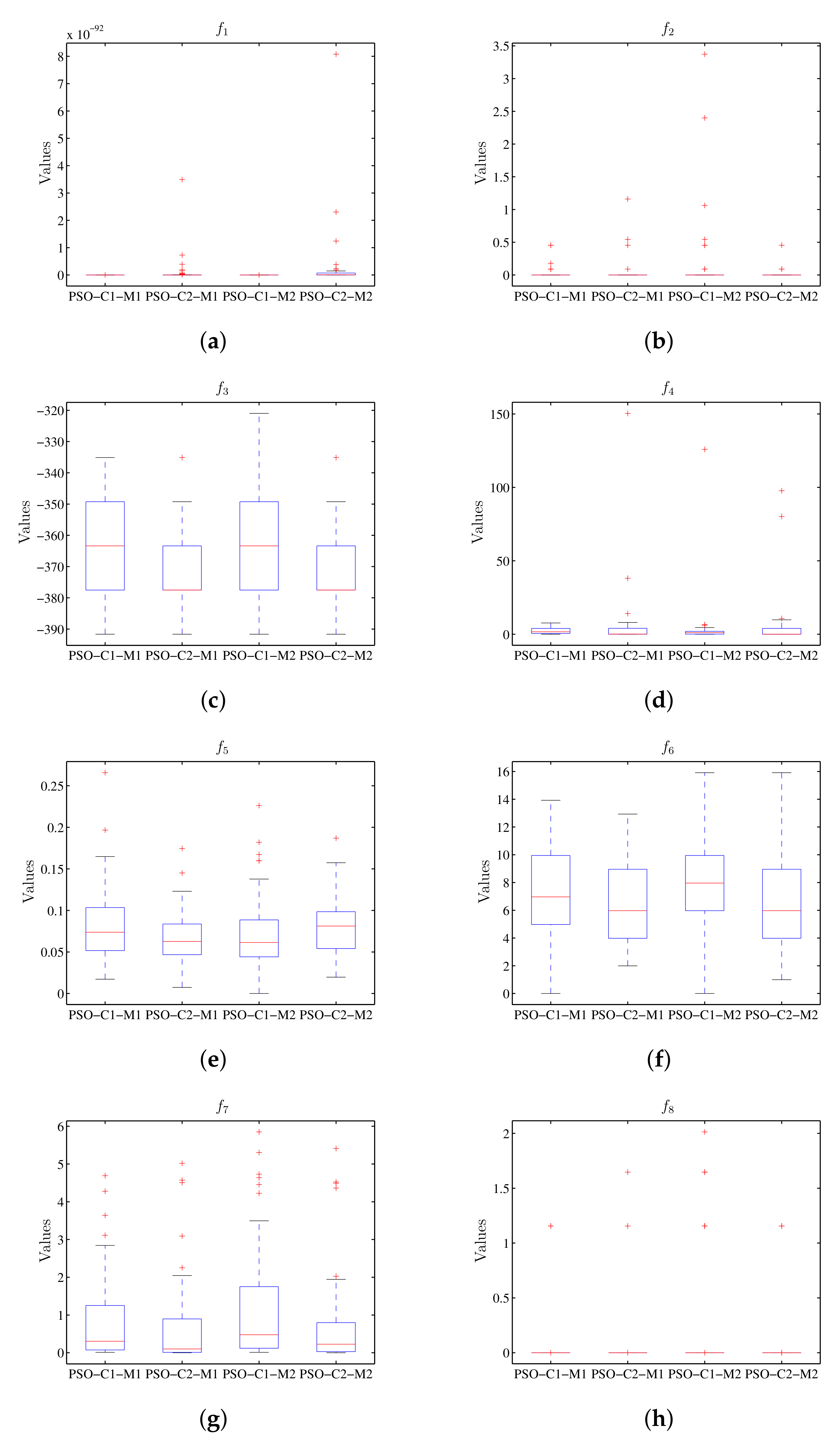
STD	0.35006	0.28167	0.55746	0.27712

and

Table 11. Statistical results for the execution time using PSO.

$f_1$	PSO-C1-M1	PSO-C2-M1	PSO-C1-M2	PSO-C2-M2
Max	4.6436	4.7827	4.3586	3.9628
Min	4.466	4.4134	3.5466	3.4743
Average	4.5714	4.4524	3.6805	3.5202
STD	0.055407	0.052652	0.19825	0.10977
$f_2$	PSO-C1-M1	PSO-C2-M1	PSO-C1-M2	PSO-C2-M2
Max	23.016	23.072	18.011	17.645
Min	22.316	22.126	16.911	16.916
Average	22.479	22.46	17.142	17.17
STD	0.14235	0.37272	0.22887	0.21337
$f_3$	PSO-C1-M1	PSO-C2-M1	PSO-C1-M2	PSO-C2-M2
Max	10.115	10.237	7.9032	7.8065
Min	9.9116	9.9536	7.3107	7.3321
Average	9.9801	10.03	7.3871	7.4062
STD	0.038899	0.045719	0.1402	0.12795
$f_4$	PSO-C1-M1	PSO-C2-M1	PSO-C1-M2	PSO-C2-M2
Max	6.7835	6.3802	7.1389	5.6697
Min	5.9945	5.9169	5.083	4.9944
Average	6.3626	6.1397	5.5549	5.2585
STD	0.17224	0.073056	0.36878	0.175
$f_5$	PSO-C1-M1	PSO-C2-M1	PSO-C1-M2	PSO-C2-M2
Max	21.211	21.321	6.8068	7.8462
Min	20.771	20.815	6.2976	6.3105
Average	20.893	21.037	6.3604	6.502
STD	0.10099	0.063159	0.087315	0.42114
$f_6$	PSO-C1-M1	PSO-C2-M1	PSO-C1-M2	PSO-C2-M2
Max	5.253	4.9498	4.5053	4.5329
Min	4.8052	4.7852	4.0516	4.0585
Average	4.8528	4.8239	4.1035	4.1364
STD	0.066958	0.036578	0.096493	0.1393
$f_7$	PSO-C1-M1	PSO-C2-M1	PSO-C1-M2	PSO-C2-M2
Max	7.0562	7.6148	6.3973	6.1467
Min	6.3352	6.3872	5.4016	5.4081
Average	6.5793	6.5748	5.7444	5.6745
STD	0.12996	0.18931	0.27627	0.18781
$f_8$	PSO-C1-M1	PSO-C2-M1	PSO-C1-M2	PSO-C2-M2
Max	8.1745	8.0003	7.0702	6.945
Min	7.3989	7.4915	6.2898	6.3109
Average	7.5151	7.5544	6.3969	6.3699
STD	0.13768	0.068633	0.16506	0.1237

display the statistical results for the value of the target function and the run-time for the PSO algorithm. The stem and leaf diagrams of the results can be seen in Figure 12 and Figure 13 for the values of the objective function and the execution time respectively. As observed in Figure 12, the value of the target function is not affected by the distributed processing scheme, while the run-time is reduced by using this schema (Figure 13).

8.4. Algorithm Comparison

It is worth pointing that this work is focused in the observations of the changes amidst the execution of each algorithm in the machines employed (M1 and M2); therefore, the results are presented separately for each algorithm; nevertheless, it is also important to bear in mind that after defining the hardware to implement the experiments, the study should be focused on the algorithm comparison (variation among them), which requires the organization of the results in a single table. As an example,

Table 12. General statistical results for the value of the objective function.

$f_1$	GA-C1-M1	GA-C2-M1	GA-C1-M2	GA-C2-M2	DE-C1-M1	DE-C2-M1	DE-C1-M2	DE-C2-M2	PSO-C1-M1	PSO-C2-M1	PSO-C1-M2	PSO-C2-M2
Max	803.1	851.1	693.48	878.87	$3.10\times {10}^{-36}$	2189.2	$6.75\times {10}^{-36}$	3135.8	$\mathbf{3.45}\times {\mathbf{10}}^{-\mathbf{128}}$	$3.49\times {10}^{-92}$	$2.01\times {10}^{-127}$	$8.08\times {10}^{-92}$
Min	110.12	231.66	96.881	198.67	$1.19\times {10}^{-38}$	33.487	$3.85\times {10}^{-39}$	5.1453	$\mathbf{4.01}\times {\mathbf{10}}^{-\mathbf{136}}$	$1.16\times {10}^{-99}$	$5.73\times {10}^{-136}$	$4.03\times {10}^{-100}$
Average	396.34	512.71	363.63	524.55	$4.45\times {10}^{-37}$	637.3	$5.60\times {10}^{-37}$	738.21	$\mathbf{2.37}\times {\mathbf{10}}^{-\mathbf{129}}$	$1.05\times {10}^{-93}$	$7.64\times {10}^{-129}$	$2.69\times {10}^{-93}$
STD	164.16	145.59	165.86	165.07	$6.88\times {10}^{-37}$	508.86	$1.18\times {10}^{-36}$	680.65	$\mathbf{6.88}\times {\mathbf{10}}^{-\mathbf{129}}$	$5.03\times {10}^{-93}$	$3.16\times {10}^{-128}$	$1.19\times {10}^{-92}$
$f_2$	GA-C1-M1	GA-C2-M1	GA-C1-M2	GA-C2-M2	DE-C1-M1	DE-C2-M1	DE-C1-M2	DE-C2-M2	PSO-C1-M1	PSO-C2-M1	PSO-C1-M2	PSO-C2-M2
Max	4.0682	2.8756	4.1886	2.9012	$\mathbf{1.50}\times {\mathbf{10}}^{-\mathbf{32}}$	5.303	$\mathbf{1.50}\times {\mathbf{10}}^{-\mathbf{32}}$	4.4089	0.45432	1.1605	3.3738	0.45432
Min	0.43532	0.73858	0.50167	0.49925	$\mathbf{1.50}\times {\mathbf{10}}^{-\mathbf{32}}$	0.33872	$\mathbf{1.50}\times {\mathbf{10}}^{-\mathbf{32}}$	0.31488	$\mathbf{1.50}\times {\mathbf{10}}^{-\mathbf{32}}$	$\mathbf{1.50}\times {\mathbf{10}}^{-\mathbf{32}}$	$\mathbf{1.50}\times {\mathbf{10}}^{-\mathbf{32}}$	$\mathbf{1.50}\times {\mathbf{10}}^{-\mathbf{32}}$
Average	2.0062	1.6742	1.7204	1.6712	$\mathbf{1.50}\times {\mathbf{10}}^{-\mathbf{32}}$	1.8351	$\mathbf{1.50}\times {\mathbf{10}}^{-\mathbf{32}}$	1.6916	0.036212	0.044963	0.18755	0.023545
STD	1.094	0.43556	0.91603	0.49293	$\mathbf{2.76}\times {\mathbf{10}}^{-\mathbf{48}}$	1.2641	$8.29\times {10}^{-48}$	0.99901	0.11155	0.18929	0.60021	0.091378
$f_3$	GA-C1-M1	GA-C2-M1	GA-C1-M2	GA-C2-M2	DE-C1-M1	DE-C2-M1	DE-C1-M2	DE-C2-M2	PSO-C1-M1	PSO-C2-M1	PSO-C1-M2	PSO-C2-M2
Max	−361.86	−369.18	−360.01	−366.04	$-\mathbf{377.52}$	−282.82	$-\mathbf{377.52}$	−276.36	−335.11	−335.11	−320.98	−335.11
Min	−385.82	−390.21	−389.06	−385.25	$-\mathbf{391.66}$	−362.53	$-\mathbf{391.66}$	−379.17	$-\mathbf{391.66}$	$-\mathbf{391.66}$	$-\mathbf{391.66}$	$-\mathbf{391.66}$
Average	−376.93	−378.57	−377.46	−378.18	−390.53	−322.34	$-\mathbf{391.1}$	−324.16	−363.95	−371.02	−365.37	−371.02
STD	5.3254	4.3697	5.5337	4.2567	3.8741	17.26	$\mathbf{2.7983}$	24.568	17.127	15.698	17.608	14.898
$f_4$	GA-C1-M1	GA-C2-M1	GA-C1-M2	GA-C2-M2	DE-C1-M1	DE-C2-M1	DE-C1-M2	DE-C2-M2	PSO-C1-M1	PSO-C2-M1	PSO-C1-M2	PSO-C2-M2
Max	$7.48\times {10}^5$	$2.67\times {10}^5$	$6.51\times {10}^5$	$2.79\times {10}^5$	$\mathbf{3.9866}$	$5.90\times {10}^5$	$\mathbf{3.9866}$	$2.81\times {10}^5$	7.7008	150.43	125.9	97.773
Min	11809	22674	10592	14904	$\mathbf{0}$	221.75	$1.05\times {10}^{-29}$	85.7	0.001011	0.00075109	$9.36\times {10}^{-5}$	$8.22\times {10}^{-5}$
Average	$2.18\times {10}^5$	$1.28\times {10}^5$	$2.03\times {10}^5$	$1.19\times {10}^5$	0.31893	79546	$\mathbf{0.079732}$	51649	2.3245	5.2944	4.0551	5.0642
STD	$1.81\times {10}^5$	61355	$1.61\times {10}^5$	59792	1.0925	$1.32\times {10}^5$	$\mathbf{0.56379}$	71056	2.2494	21.749	17.666	17.601
$f_5$	GA-C1-M1	GA-C2-M1	GA-C1-M2	GA-C2-M2	DE-C1-M1	DE-C2-M1	DE-C1-M2	DE-C2-M2	PSO-C1-M1	PSO-C2-M1	PSO-C1-M2	PSO-C2-M2
Max	1.0079	0.90574	1.0422	0.95218	0.47846	0.90603	0.54541	0.8534	0.2658	$\mathbf{0.17454}$	0.22621	0.18699
Min	0.13795	0.51898	0.13518	0.4226	0.0098573	0.11603	$\mathbf{0}$	0.14461	0.017236	0.007396	$\mathbf{0}$	0.01969
Average	0.62559	0.72619	0.64354	0.72477	0.17114	0.37272	0.15415	0.36911	0.082166	$\mathbf{0.067271}$	0.073552	0.081583
STD	0.29169	0.10053	0.27751	0.11398	0.12517	0.16561	0.12216	0.17738	0.045771	$\mathbf{0.032932}$	0.046	0.036983
$f_6$	GA-C1-M1	GA-C2-M1	GA-C1-M2	GA-C2-M2	DE-C1-M1	DE-C2-M1	DE-C1-M2	DE-C2-M2	PSO-C1-M1	PSO-C2-M1	PSO-C1-M2	PSO-C2-M2
Max	26.967	22.369	26.161	23.734	18.436	61.339	22.189	89.495	13.929	$\mathbf{12.934}$	15.919	15.919
Min	9.0212	11.351	6.8412	7.9241	1.9899	7.284	2.9849	7.5864	$\mathbf{0}$	1.9899	$\mathbf{0}$	0.99496
Average	18.404	17.323	16.87	17.45	7.6318	26.926	8.9962	30.295	7.1836	$\mathbf{6.507}$	7.9995	6.6861
STD	4.2545	$\mathbf{2.6509}$	4.1317	3.2635	3.5215	12.042	4.4606	15.282	3.1674	2.942	3.5275	3.5107
$f_7$	GA-C1-M1	GA-C2-M1	GA-C1-M2	GA-C2-M2	DE-C1-M1	DE-C2-M1	DE-C1-M2	DE-C2-M2	PSO-C1-M1	PSO-C2-M1	PSO-C1-M2	PSO-C2-M2
Max	15.554	15.825	15.913	16.091	0.00025313	26.502	$\mathbf{0.00023235}$	31.125	4.6907	5.0196	5.8513	5.4093
Min	5.81	9.5476	6.1036	9.749	$4.48\times {10}^{-6}$	6.2426	$2.78\times {10}^{-6}$	7.3592	0.010729	$5.78\times {10}^{-23}$	0.010729	$\mathbf{1.02}\times {\mathbf{10}}^{-\mathbf{23}}$
Average	9.7471	13.107	9.4184	13.142	$\mathbf{3.18}\times {\mathbf{10}}^{-\mathbf{5}}$	16.616	$4.16\times {10}^{-5}$	16.469	0.89475	0.72333	1.2073	0.74679
STD	2.1818	1.3576	2.1384	1.3547	$\mathbf{3.89}\times {\mathbf{10}}^{-\mathbf{5}}$	4.8337	$4.69\times {10}^{-5}$	4.8209	1.2023	1.2346	1.6043	1.2825
$f_8$	GA-C1-M1	GA-C2-M1	GA-C1-M2	GA-C2-M2	DE-C1-M1	DE-C2-M1	DE-C1-M2	DE-C2-M2	PSO-C1-M1	PSO-C2-M1	PSO-C1-M2	PSO-C2-M2
Max	3.4624	5.2211	3.8739	5.3901	$\mathbf{3.11}\times {\mathbf{10}}^{-\mathbf{15}}$	15.395	$\mathbf{3.11}\times {\mathbf{10}}^{-\mathbf{15}}$	13.672	1.1551	1.6462	2.0133	1.1551
Min	0.88282	3.3081	1.2655	3.0742	$\mathbf{3.11}\times {\mathbf{10}}^{-\mathbf{15}}$	1.8371	$\mathbf{3.11}\times {\mathbf{10}}^{-\mathbf{15}}$	2.0741	$\mathbf{3.11}\times {\mathbf{10}}^{-\mathbf{15}}$	$\mathbf{3.11}\times {\mathbf{10}}^{-\mathbf{15}}$	$\mathbf{3.11}\times {\mathbf{10}}^{-\mathbf{15}}$	$\mathbf{3.11}\times {\mathbf{10}}^{-\mathbf{15}}$
Average	2.4774	4.2857	2.7235	4.253	$\mathbf{3.11}\times {\mathbf{10}}^{-\mathbf{15}}$	8.5284	$\mathbf{3.11}\times {\mathbf{10}}^{-\mathbf{15}}$	7.9863	0.11551	0.056027	0.26784	0.069309
STD	0.5349	0.44425	0.55014	0.53566	$\mathbf{0}$	2.8974	$\mathbf{0}$	3.0219	0.35006	0.28167	0.55746	0.27712

displays the summary of results considering the objective function while

Table 13. General statistical results for the run time.

$f_1$	GA-C1-M1	GA-C2-M1	GA-C1-M2	GA-C2-M2	DE-C1-M1	DE-C2-M1	DE-C1-M2	DE-C2-M2	PSO-C1-M1	PSO-C2-M1	PSO-C1-M2	PSO-C2-M2
Max	24.144	14.818	23.045	13.121	16.266	7.5975	13.654	5.8533	4.6436	4.7827	4.3586	$\mathbf{3.9628}$
Min	21.58	14.109	19.585	12.583	15.431	6.7975	11.854	5.2711	4.466	4.4134	3.5466	$\mathbf{3.4743}$
Average	22.567	14.376	20.548	12.98	15.772	7.038	12.245	5.343	4.5714	4.4524	3.6805	$\mathbf{3.5202}$
STD	0.83158	0.21588	0.78465	0.14111	0.18457	0.14197	0.38329	0.078526	0.055407	$\mathbf{0.052652}$	0.19825	0.10977
$f_2$	GA-C1-M1	GA-C2-M1	GA-C1-M2	GA-C2-M2	DE-C1-M1	DE-C2-M1	DE-C1-M2	DE-C2-M2	PSO-C1-M1	PSO-C2-M1	PSO-C1-M2	PSO-C2-M2
Max	53.419	33.995	43.846	28.084	57.416	23.251	34.549	$\mathbf{15.018}$	23.016	23.072	18.011	17.645
Min	52.5	32.746	42.469	27.325	48.193	20.763	33.857	$\mathbf{14.653}$	22.316	22.126	16.911	16.916
Average	52.705	33.576	43.305	27.68	49.606	21.304	34.325	$\mathbf{14.75}$	22.479	22.46	17.142	17.17
STD	0.19373	0.45674	0.40224	0.29811	1.8648	0.58789	0.20726	$\mathbf{0.049601}$	0.14235	0.37272	0.22887	0.21337
$f_3$	GA-C1-M1	GA-C2-M1	GA-C1-M2	GA-C2-M2	DE-C1-M1	DE-C2-M1	DE-C1-M2	DE-C2-M2	PSO-C1-M1	PSO-C2-M1	PSO-C1-M2	PSO-C2-M2
Max	33.675	21.241	27.961	16.951	27.869	12.068	18.801	8.2856	10.115	10.237	7.9032	$\mathbf{7.8065}$
Min	32.444	20.753	27.693	16.249	26.586	11.451	18.492	8.1547	9.9116	9.9536	$\mathbf{7.3107}$	7.3321
Average	32.656	20.933	27.829	16.625	27.24	11.765	18.633	8.2207	9.9801	10.03	$\mathbf{7.3871}$	7.4062
STD	0.2189	0.12987	0.051181	0.19769	0.23964	0.13481	0.068874	$\mathbf{0.031299}$	0.038899	0.045719	0.1402	0.12795
$f_4$	GA-C1-M1	GA-C2-M1	GA-C1-M2	GA-C2-M2	DE-C1-M1	DE-C2-M1	DE-C1-M2	DE-C2-M2	PSO-C1-M1	PSO-C2-M1	PSO-C1-M2	PSO-C2-M2
Max	26.432	17.195	23.177	14.662	20.083	9.6074	15.165	6.5915	6.7835	6.3802	7.1389	$\mathbf{5.6697}$
Min	25.832	16.809	22.28	14.579	18.842	8.8058	14.626	6.4609	5.9945	5.9169	5.083	$\mathbf{4.9944}$
Average	26.12	16.988	22.806	14.625	19.604	8.9937	14.947	6.5287	6.3626	6.1397	5.5549	$\mathbf{5.2585}$
STD	0.12577	0.10671	0.3793	$\mathbf{0.021441}$	0.22143	0.13871	0.17267	0.032574	0.17224	0.073056	0.36878	0.175
$f_5$	GA-C1-M1	GA-C2-M1	GA-C1-M2	GA-C2-M2	DE-C1-M1	DE-C2-M1	DE-C1-M2	DE-C2-M2	PSO-C1-M1	PSO-C2-M1	PSO-C1-M2	PSO-C2-M2
Max	56.463	37.643	25.431	15.981	28.155	12.564	21.205	7.9327	21.211	21.321	$\mathbf{6.8068}$	7.8462
Min	51.667	32.043	24.527	15.403	21.609	9.5708	16.104	7.3504	20.771	20.815	$\mathbf{6.2976}$	6.3105
Average	52.609	32.336	25.207	15.777	23.728	10.065	16.841	7.4283	20.893	21.037	$\mathbf{6.3604}$	6.502
STD	0.98871	0.79033	0.28878	0.2308	1.3008	0.57603	0.82097	0.080032	0.10099	$\mathbf{0.063159}$	0.087315	0.42114
$f_6$	GA-C1-M1	GA-C2-M1	GA-C1-M2	GA-C2-M2	DE-C1-M1	DE-C2-M1	DE-C1-M2	DE-C2-M2	PSO-C1-M1	PSO-C2-M1	PSO-C1-M2	PSO-C2-M2
Max	23.767	15.585	20.968	13.325	20.134	10.592	15.865	7.8398	5.253	4.9498	$\mathbf{4.5053}$	4.5329
Min	22.686	14.818	20.182	12.843	16.432	7.5325	12.441	5.7978	4.8052	4.7852	$\mathbf{4.0516}$	4.0585
Average	23.014	14.918	20.424	12.898	17.298	8.1412	12.988	6.0956	4.8528	4.8239	$\mathbf{4.1035}$	4.1364
STD	0.22193	0.13802	0.30039	0.063915	0.59429	0.8543	0.66904	0.54322	0.066958	$\mathbf{0.036578}$	0.096493	0.1393
$f_7$	GA-C1-M1	GA-C2-M1	GA-C1-M2	GA-C2-M2	DE-C1-M1	DE-C2-M1	DE-C1-M2	DE-C2-M2	PSO-C1-M1	PSO-C2-M1	PSO-C1-M2	PSO-C2-M2
Max	26.147	17.097	23.718	15.003	20.159	11.566	15.484	8.8737	7.0562	7.6148	6.3973	$\mathbf{6.1467}$
Min	25.505	16.514	23.571	14.883	19.054	8.5482	15.042	6.7808	6.3352	6.3872	$\mathbf{5.4016}$	5.4081
Average	25.675	16.608	23.661	14.943	19.593	9.0394	15.397	7.171	6.5793	6.5748	5.7444	$\mathbf{5.6745}$
STD	0.1198	0.087461	0.031198	$\mathbf{0.023558}$	0.33105	0.70994	0.088293	0.57938	0.12996	0.18931	0.27627	0.18781
$f_8$	GA-C1-M1	GA-C2-M1	GA-C1-M2	GA-C2-M2	DE-C1-M1	DE-C2-M1	DE-C1-M2	DE-C2-M2	PSO-C1-M1	PSO-C2-M1	PSO-C1-M2	PSO-C2-M2
Max	28.488	18.888	25.426	16.091	23.642	12.882	17.531	7.8927	8.1745	8.0003	7.0702	$\mathbf{6.945}$
Min	27.7	17.862	25.294	15.904	22.782	9.805	17.011	7.4364	7.3989	7.4915	$\mathbf{6.2898}$	6.3109
Average	27.885	18.179	25.365	15.948	23.23	10.159	17.413	7.5943	7.5151	7.5544	6.3969	$\mathbf{6.3699}$
STD	0.15947	0.21193	0.032987	$\mathbf{0.029009}$	0.19133	0.44989	0.13786	0.069855	0.13768	0.068633	0.16506	0.1237

displays the results for the execution time.

Usually, these tables highlight the best value reached by one of the algorithms (for each test function) in a way that a global comparison can be made for both the obtained value of the objective function and the execution time for the algorithms employed. Table 12 and Table 13 show an example each of the way by which the best obtained values can be noted.

8.5. Execution Time Analysis

As previously observed in the results obtained, the values of the target function for configurations C1 and C2 are not affected by the type of processing system—executed in M1 or M2, but the processing time is affected. For the above, this section only performs an analysis of the execution times of the algorithms, this in order to observe the difference present in the execution time.

First,

Table 14. Total values for the execution time using a genetic algorithm.

f	GA-C1-M1	GA-C2-M1	GA-C1-M2	GA-C2-M2
$f_1$	1128.4	718.81	1027.4	649.02
$f_2$	2635.3	1678.8	2165.2	1384
$f_3$	1632.8	1046.7	1391.4	831.26
$f_4$	1306	849.38	1140.3	731.26
$f_5$	2630.5	1616.8	1260.3	788.87
$f_6$	1150.7	745.89	1021.2	644.9
$f_7$	1283.8	830.4	1183	747.14
$f_8$	1394.2	908.95	1268.2	797.4
Total	13,162	839.6	10,457	6574

contains the total run-time values for each configuration of the GA algorithm in each target function. Secondly, the total results for the time of execution of the DE algorithm can be seen in

Table 15. Total values for the execution time using differential evolution.

f	DE-C1-M1	DE-C2-M1	DE-C1-M2	DE-C2-M2
$f_1$	788.58	351.9	612.27	267.15
$f_2$	2480.3	1065.2	1716.3	737.48
$f_3$	1362	588.25	931.63	411.04
$f_4$	980.19	449.69	747.37	326.44
$f_5$	1186.4	503.27	842.07	371.42
$f_6$	864.88	407.06	649.41	304.78
$f_7$	979.64	451.97	769.87	358.55
$f_8$	1161.5	507.97	870.66	379.72
Total	9803.5	4325.3	7139.6	3156.6

. Finally, the total run-time values of the PSO algorithm are presented in the

Table 16. Total values for the execution time using particle swarm optimization.

f	PSO-C1-M1	PSO-C2-M1	PSO-C1-M2	PSO-C2-M2
$f_1$	228.57	222.62	184.03	176.01
$f_2$	1124	1123	857.1	858.52
$f_3$	499.01	501.5	369.35	370.31
$f_4$	318.13	306.98	277.74	262.93
$f_5$	1044.6	1051.8	318.02	325.1
$f_6$	242.64	241.19	205.18	206.82
$f_7$	328.97	328.74	287.22	283.73
$f_8$	375.75	377.72	319.84	318.5
Total	4161.7	4153.6	2818.5	2801.9

.

The total values for the execution times of each algorithm can be seen in

Table 17. Total values for the execution time of the algorithms (in seconds).

Algorithm	M1	M2	Difference	Percentage TG
GA	21,557	17,031	4526	$10.28\%$
DE	14,129	10,296	3833	$8.72\%$
PSO	8315	5620	2695	$6.12\%$
Total	44,001	32,947	11,054	$25.12\%$

. In this way, a total difference of 11,054 s that corresponds to 3.07 h in the execution of all algorithms can be seen, equivalent to $25.12\%$. In this order, the percentage corresponds to time gained for GA which is $10.28\%$ for DE $8.72\%$ and $6.12\%$ for PSO. The percentage of time gained (TG) is calculated using the following equation:

$$\mathrm{TG}=\frac{\mathrm{Difference}}{\mathrm{Total}\mathrm{time}\mathrm{for}\mathrm{M}1}100\%$$

(5)

9. Discussion

In the results, it can be seen that on average, the values obtained from the objective functions are not affected, which allows the experiments to be reproduced on different machines. It is also appreciated that when using the CECAD machine the processing time decreases, which was sought to verify with this work.

It should be noted that in this work that the effects of the parameters of the algorithms on the objective function were not closely analyzed, since we sought to observe that the same result was obtained on average for the two machines used. In order to carry out performance tests between algorithms, we first seek to establish the most appropriate computing system.

Although we observed the advantage that the virtualized distributed processing system has for the execution of the algorithms considered, only one possible configuration offered by CECAD was used, which was limited to the requests of the researchers at the time of executing the algorithms. To consider this aspect in additional work, the availability of resources held in CECAD for an average researcher as well as the time allocated for their use can be included in the study. About this, it is necessary to take in account the request in the way that the administration can manage these resources and not leave other researchers without access.

For further research, the report [50,51] can be taken as a reference since greater size and complexity of the test functions can be considered for testing the efficacy of the distributed system. In the first place, the report [50] can be considered for the testing of bio-inspired algorithms using parallel PC cluster systems for large-scale multimodal functions; secondly, the functions discussed in [51] can be used to observe the problem complexity.

Considering the restrictions of CECAD for extending this work, other computing systems can be considered, such as a non-homogeneous cluster of PCs; and a cluster with mini PCs, such as small single-board computers like Raspberry Pi. Additionally, we could consider evaluate various ways of distributing the execution of bio-inspired optimization algorithms.

10. Conclusions

Aiming at a wide range of experiments, the tests were performed with three bio-inspired algorithms under different parameter configurations using eight test functions which had different characteristics. To have comparable results, the well-known bio-inspired optimization algorithms GA, DE, and PSO were used.

The results showed that the value of the target function is not affected by the distributed virtualization scheme, while the run-time is reduced by using the distributed virtualization system. Thus, the algorithms can be executed on different machines without affecting the result.

Distributed and virtualization technologies can optimize performance and simplify the management of the information infrastructure, as they do when running bio-inspired optimization algorithms. As seen in the results, the processing time decreases when using the CECAD.

In the development of this work it was observed that the distributed virtualization system under consideration is an adequate platform for the execution of bio-inspired optimization algorithms. However, in the case of CECAD, the amount of resources and the computing capacity are subjected to the number of requests made by the researchers.