Hierarchical Cubical Tensor Decomposition through Low Complexity Orthogonal Transforms

Abstract

In this work, new approaches are proposed for the 3D decomposition of a cubical tensor of size N × N × N for N = 2ⁿ through hierarchical deterministic orthogonal transforms with low computational complexity, whose kernels are based on the Walsh-Hadamard Transform (WHT) and the Complex Hadamard Transform (CHT). On the basis of the symmetrical properties of the real and complex Walsh-Hadamard matrices are developed fast computational algorithms whose computational complexity is compared with that of the famous deterministic transforms: the 3D Fast Fourier Transform, the 3D Discrete Wavelet Transform and the statistical Hierarchical Tucker decomposition. The comparison results show the lower computational complexity of the offered algorithms. Additionally, they ensure the high energy concentration of the original tensor into a small number of coefficients of the so calculated transformed spectrum tensor. The main advantage of the proposed algorithms is the reduction of the needed calculations due to the low number of hierarchical levels compared to the significant number of iterations needed to achieve the required decomposition accuracy based on the statistical methods. The choice of the 3D hierarchical decomposition is defined by the requirements and limitations related to the corresponding application area.

1. Introduction

The famous tensor decompositions—Canonical Polyadic Decomposition (CPD), Higher-Order Singular Value Decomposition (HOSVD) [1,2,3], Tensor Trains Decomposition (TTD) [4], and Hierarchical Tucker decomposition (H Tucker) [5] - and their modifications [6] are based on the calculation of the eigen values and eigen vectors of the decomposed tensor. Their basic advantage is that they are optimum with respect to the Mean Square Error (MSE) of the approximation in the case of the truncation of the low-energy decomposition components. For the calculation of the retained components are used various iterative methods (the power method [7], the Jacoby method [8], etc.), which require relatively high numbers of calculations to achieve the needed approximation accuracy.

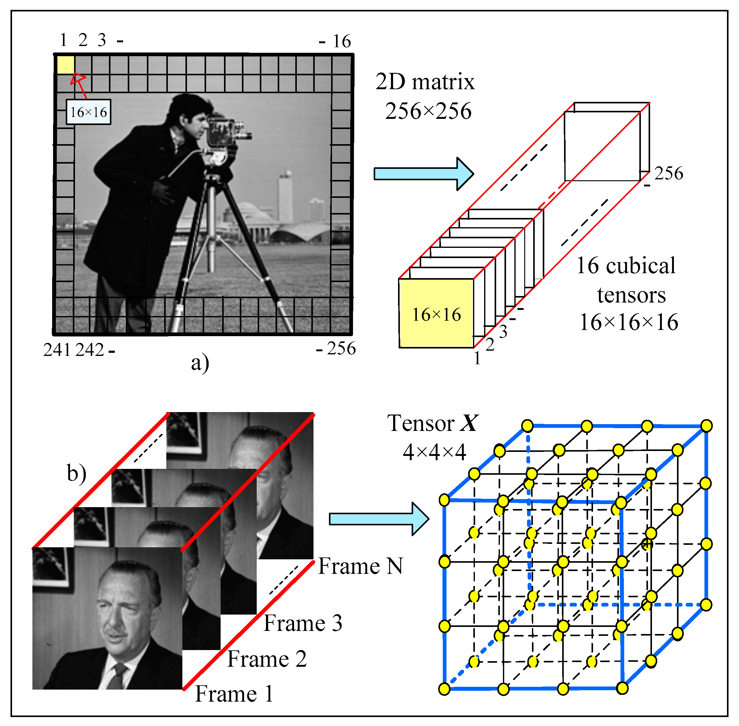
As an alternative, in this work are presented new hierarchical approaches for 3D tensor decomposition, based on well-known deterministic orthogonal transforms: the Walsh-Hadamard Transform (WHT) [9,10,11,12] and the Complex Hadamard Transform (CHT) [13]. The offered decompositions are not optimum with respect to MSE minimization, but due to the lack of iterations, they have low Computational Complexity (CC), and as a result, they are suitable for the fast processing of the 3D tensors obtained, for example, from single or sequences of 2D correlated images. In the first case, each single 2D image is divided into N² blocks of size N × N for N = 2ⁿ, from which is obtained a sequence of N cubical tensors, each of size N × N × N. In the second case, from each sequence of N 2D images of size N × N is obtained a single cubical tensor of size N × N × N. Examples for the transformation of a single 2D image and of a sequence of 2D video frames into a cubical (3D) tensor are shown on Figure 1.

The presented approach for fast hierarchical cubical tensor decomposition is applicable not only for images but also for various kinds of multidimensional signals (medical, seismic, spectrometric, etc.) and big data analysis. In the next sections, Section 2, Section 3, Section 4 and Section 5, are presented the proposed algorithms for 1D Hierarchical Fast Walsh-Hadamard Transform (1D-FWHT), 1D Hierarchical Fast Complex Hadamard Transform (1D-FCHT), and the corresponding 3D Hierarchical Fast real and complex transforms (3D-FWHT and 3D-FCHT). In Section 6 is shown a comparative analysis of the CC of the presented algorithms for hierarchical orthogonal tensor transforms, with respect to the famous deterministic and statistical transforms: the 3D Fast Fourier Transform (3D-FFT), 3D Discrete Wavelet Transform (3D-DWT) and Hierarchical Tucker Decomposition (H-Tucker). The last section, Section 7, contains the conclusions.

In Appendix A.1 and Appendix A.2 is given the factorization of the matrices for the n-level one-dimensional fast hierarchical transforms 1D-FWHT and 1D-FCHT.

2. One-Dimensional Hierarchical Fast Walsh-Hadamard Transform

The following symbols are introduced for tensors, matrices and vectors, respectively: X for a tensor, X for a matrix and $\overrightarrow{\mathrm{x}}$ for a vector.

The forward and inverse 1D Walsh-Hadamard Transform (1D-WHT) (frequency-ordered) is represented in scalar form by the equations below [9,10,11]:

$$\mathrm{s}(\mathrm{u})={\displaystyle \sum _{\mathrm{i}=0}^{\mathrm{N}-1}\mathrm{x}(\mathrm{i}) \mathrm{wal}(\mathrm{i},\mathrm{u})}; \mathrm{x}(\mathrm{i})=(1/\mathrm{N}){\displaystyle \sum _{\mathrm{u}=0}^{\mathrm{N}-1}\mathrm{s}(\mathrm{u}) \mathrm{wal}(\mathrm{i},\mathrm{u})} \mathrm{for} \mathrm{i}, \mathrm{u}=0,1,\dots ,\mathrm{N}-1,$$

(1)

where N = 2ⁿ and x(i) and s(u) are, respectively, the N-dimensional discrete signal and its spectrum. The discrete Wash functions are defined by the following relations [10,12]:

$$\mathrm{wal}(\mathrm{i},\mathrm{u})={(-1)}^{{\displaystyle \sum _{\mathrm{r}=0}^{\mathrm{n}-1}{\mathrm{q}}_{\mathrm{r}}(\mathrm{i}){\mathrm{u}}_{\mathrm{r}}}}; {\mathrm{q}}_{\mathrm{r}}(\mathrm{i})={\mathrm{i}}_{\mathrm{n}-\mathrm{r}}\oplus {\mathrm{i}}_{\mathrm{n}-\mathrm{r}-1} \mathrm{for} \mathrm{r}=1,2,\dots ,\mathrm{n}-1; {\mathrm{q}}_0(\mathrm{i})={\mathrm{i}}_{\mathrm{n}-1}; \mathrm{i}={\displaystyle \sum _{\mathrm{r}=0}^{\mathrm{n}-1}{\mathrm{i}}_{\mathrm{r}}{2}^{\mathrm{r}}}, \mathrm{u}={\displaystyle \sum _{\mathrm{r}=0}^{\mathrm{n}-1}{\mathrm{u}}_{\mathrm{r}}{2}^{\mathrm{r}}}.$$

(2)

Here, the operation “exclusive OR” is represented by the symbol ⊕.

The algorithm for the one-dimensional hierarchical fast Walsh-Hadamard transform (1D-FWHT) for the cubical tensor X of size N × N × N when N = 2ⁿ (a sequence of matrices X_k, each of size N × N for k = 1, 2, …,N) is presented for N = 8 (i.e., for n = 3 levels). The general case of the transform when N = 2ⁿ and n >3, is given in Appendix A.1.

The execution of the direct and inverse 1D-WHT is grounded on the basic operation “butterfly” for N = 2, in accordance with the following relations [9,11]:

$$\begin{array}{l}\mathrm{y}(1)=\mathrm{x}(1)+\mathrm{x}(2),\\ \mathrm{y}(2)=\mathrm{x}(1)-\mathrm{x}(2),\end{array} \begin{array}{l}\mathrm{x}(1)=(1/2)[\mathrm{y}(1)+\mathrm{y}(2)],\\ \mathrm{x}(2)=(1/2)[\mathrm{y}(1)-\mathrm{y}(2)].\end{array}$$

(3)

The application of the operation “butterfly” to the elements of the couples of matrices in each hierarchical level is represented by the equations below.

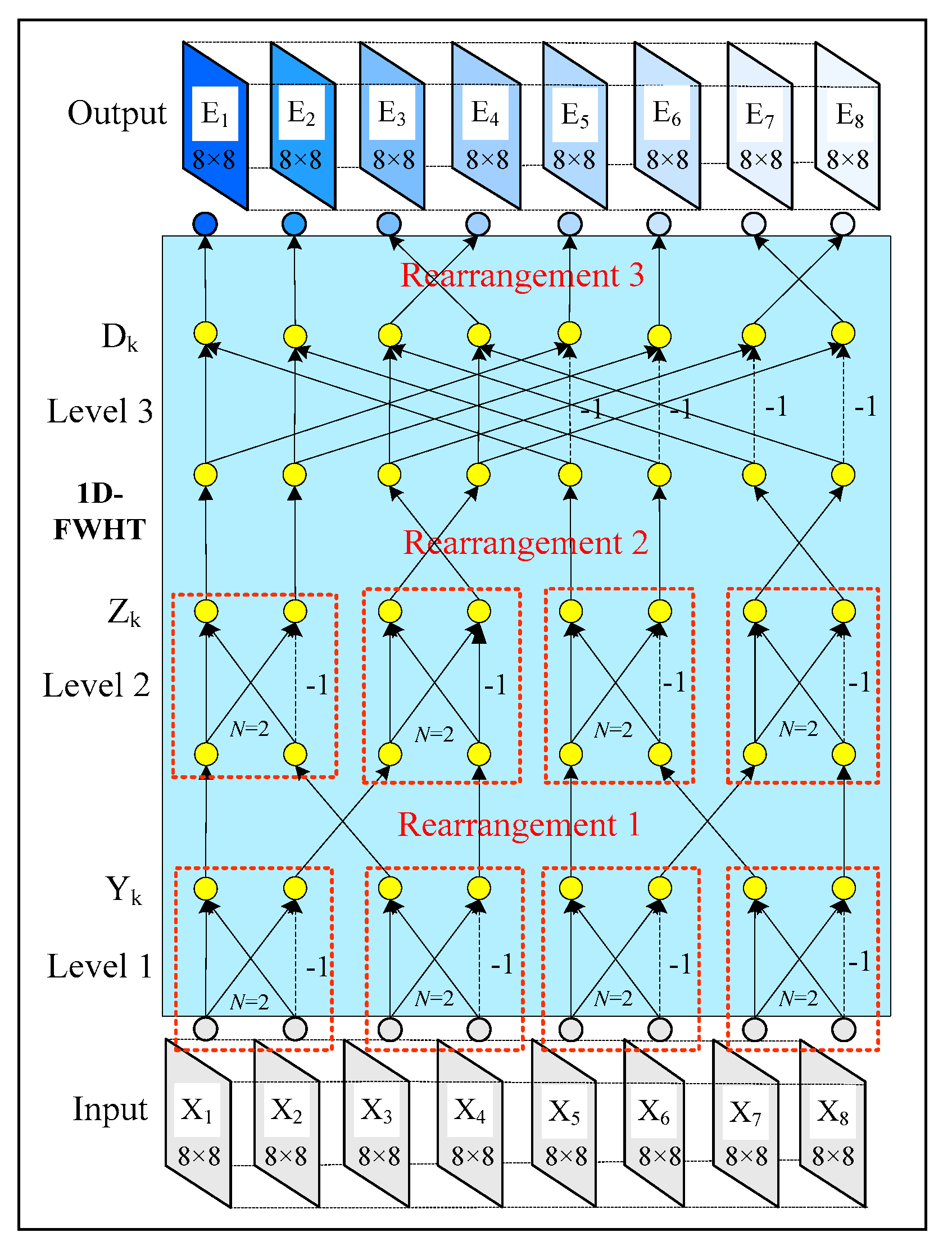
In Level 1 of the 1D-FWHT:

$$\mathrm{Y}={\mathrm{G}}_1(8)\mathrm{X}.$$

(4)

The matrix G₁(8) of size 8 × 8 is used to execute the direct 1D-WHT when N = 2 for each couple of neighbor matrices in the sequence X_k for k = 1,2, …,8. These matrices are the components of the matrix-column $\mathrm{X}={[{\mathrm{X}}_1,{\mathrm{X}}_2,{\mathrm{X}}_3,{\mathrm{X}}_4,{\mathrm{X}}_5,{\mathrm{X}}_6,{\mathrm{X}}_7,{\mathrm{X}}_8]}^{\mathrm{T}}$. From Equation (3), it follows that the matrix G₁ (8) could be represented in the following way:

$${\mathrm{G}}_1(8)=\mathrm{I}(4)\otimes \mathrm{H}(2)=\left[\begin{array}{cccc}\mathrm{H}(2)& 0& 0& 0\\ 0& \mathrm{H}(2)& 0& 0\\ 0& 0& \mathrm{H}(2)& 0\\ 0& 0& 0& \mathrm{H}(2)\end{array}\right], \mathrm{H}(2)=\left[\begin{array}{cc}1& 1\\ 1& -1\end{array}\right] -\mathrm{Hadamard} \mathrm{matrix} \mathrm{of} \mathrm{size} 2 \times 2.$$

(5)

Here, I(4) is the identity matrix of size 4 × 4, the symbol ⊗ stands for the Kroneker product of the matrices [3], and $\mathrm{Y}={[{\mathrm{Y}}_1,{\mathrm{Y}}_2,{\mathrm{Y}}_3,{\mathrm{Y}}_4,{\mathrm{Y}}_5,{\mathrm{Y}}_6,{\mathrm{Y}}_7,{\mathrm{Y}}_8]}^{\mathrm{T}}$ corresponds to the transformed matrix-column whose components are the matrices Y_k, for k = 1,2,…,8.

After the rearrangement 1 is obtained:

$$\mathrm{Y}\prime ={\mathrm{P}}_1(8)\mathrm{Y},$$

(6)

where

$${\mathrm{P}}_1(8)={\mathrm{L}}_1(4)\otimes \mathrm{I}(2)=\left[\begin{array}{cc}{\mathrm{L}}_1(4)& 0\\ 0& {\mathrm{L}}_1(4)\end{array}\right] ; {\mathrm{L}}_1(4)=\left[\begin{array}{cccc}1& 0& 0& 0\\ 0& 0& 1& 0\\ 0& 1& 0& 0\\ 0& 0& 0& 1\end{array}\right] -\mathrm{permutation} \mathrm{sub}-\mathrm{matrix} \mathrm{of} \mathrm{size} 4\times 4;$$

(7)

P₁(8)—permutation matrix of size 8 × 8; ${\mathrm{Y}}^{\prime }={[{{\mathrm{Y}}^{\prime }}_1,{{\mathrm{Y}}^{\prime }}_2,{{\mathrm{Y}}^{\prime }}_3,{{\mathrm{Y}}^{\prime }}_4,{{\mathrm{Y}}^{\prime }}_5,{{\mathrm{Y}}^{\prime }}_6,{{\mathrm{Y}}^{\prime }}_7,{{\mathrm{Y}}^{\prime }}_8]}^{\mathrm{T}}$- rearranged matrix-column with components ${{\mathrm{Y}}^{\prime }}_1={\mathrm{Y}}_1, {{\mathrm{Y}}^{\prime }}_2={\mathrm{Y}}_3, {{\mathrm{Y}}^{\prime }}_3={\mathrm{Y}}_2, {{\mathrm{Y}}^{\prime }}_4={\mathrm{Y}}_4, {{\mathrm{Y}}^{\prime }}_5={\mathrm{Y}}_5, {{\mathrm{Y}}^{\prime }}_6={\mathrm{Y}}_7, {{\mathrm{Y}}^{\prime }}_7={\mathrm{Y}}_6, {{\mathrm{Y}}^{\prime }}_8={\mathrm{Y}}_8$.

In the Level 2 of the 1D-FWHT is obtained:

$$\mathrm{Z}={\mathrm{G}}_2(8)\mathrm{Y}\prime ,$$

(8)

where G₂(8) = G₁(8) and $\mathrm{Z}={[{\mathrm{Z}}_1,{\mathrm{Z}}_2,{\mathrm{Z}}_3,{\mathrm{Z}}_4,{\mathrm{Z}}_5,{\mathrm{Z}}_6,{\mathrm{Z}}_7,{\mathrm{Z}}_8]}^{\mathrm{T}}$. The components of the matrix Z are:

$$\begin{array}{c}{\mathrm{Z}}_1={\mathrm{Y}}_1+{\mathrm{Y}}_3; {\mathrm{Z}}_2={\mathrm{Y}}_1-{\mathrm{Y}}_3; {\mathrm{Z}}_3={\mathrm{Y}}_2+{\mathrm{Y}}_4; {\mathrm{Z}}_4={\mathrm{Y}}_2-{\mathrm{Y}}_4;\\ {\mathrm{Z}}_5={\mathrm{Y}}_5+{\mathrm{Y}}_7; {\mathrm{Z}}_6={\mathrm{Y}}_5-{\mathrm{Y}}_7; {\mathrm{Z}}_7={\mathrm{Y}}_6+{\mathrm{Y}}_8; {\mathrm{Z}}_8={\mathrm{Y}}_6-{\mathrm{Y}}_8.\end{array}$$

After the rearrangement 2 is obtained:

$$\mathrm{Z}\prime ={\mathrm{P}}_2(8)\mathrm{Z},$$

(9)

where

$${\mathrm{P}}_2(8)={\mathrm{L}}_2(4)\otimes \mathrm{I}(2)=\left[\begin{array}{cc}{\mathrm{L}}_2(4)& 0\\ 0& {\mathrm{L}}_2(4)\end{array}\right]; {\mathrm{L}}_2(4)=\left[\begin{array}{cccc}1& 0& 0& 0\\ 0& 1& 0& 0\\ 0& 0& 0& 1\\ 0& 0& 1& 0\end{array}\right] -\mathrm{permutation} \mathrm{sub}-\mathrm{matrix} \mathrm{of} \mathrm{size} 4\times 4;$$

(10)

P₂(8)—permutation matrix of size 8 × 8; $\mathrm{Z}\prime ={[{{\mathrm{Z}}^{\prime }}_1,{{\mathrm{Z}}^{\prime }}_2,{{\mathrm{Z}}^{\prime }}_3,{{\mathrm{Z}}^{\prime }}_4,{{\mathrm{Z}}^{\prime }}_5,{{\mathrm{Z}}^{\prime }}_6,{{\mathrm{Z}}^{\prime }}_7,{{\mathrm{Z}}^{\prime }}_8]}^{\mathrm{T}}$- rearranged matrix-column with components ${{\mathrm{Z}}^{\prime }}_1={\mathrm{Z}}_1, {{\mathrm{Z}}^{\prime }}_2={\mathrm{Z}}_2, {{\mathrm{Z}}^{\prime }}_3={\mathrm{Z}}_4, {{\mathrm{Z}}^{\prime }}_4={\mathrm{Z}}_3, {{\mathrm{Z}}^{\prime }}_5={\mathrm{Z}}_5, {{\mathrm{Z}}^{\prime }}_6={\mathrm{Z}}_6, {{\mathrm{Z}}^{\prime }}_7={\mathrm{Z}}_8, {{\mathrm{Z}}^{\prime }}_8={\mathrm{Z}}_7$.

In the Level 3 of the 1D-FWHT is obtained:

$$\mathrm{D}={\mathrm{G}}_3(8)\mathrm{Z}\prime ,$$

(11)

where

$${\mathrm{G}}_3(8)=\mathrm{H}(2)\otimes \mathrm{I}(4)=\left[\begin{array}{cc}\mathrm{I}(4)& \mathrm{I}(4)\\ \mathrm{I}(4)& -\mathrm{I}(4)\end{array}\right] \mathrm{for} \mathrm{I}(4)=\left[\begin{array}{cccc}1& 0& 0& 0\\ 0& 1& 0& 0\\ 0& 0& 1& 0\\ 0& 0& 0& 1\end{array}\right] -\mathrm{identity} \mathrm{matrix} \mathrm{of} \mathrm{size}4\times 4;$$

(12)

$\mathrm{D}={[{\mathrm{D}}_1,{\mathrm{D}}_2,{\mathrm{D}}_3,{\mathrm{D}}_4,{\mathrm{D}}_5,{\mathrm{D}}_6,{\mathrm{D}}_7,{\mathrm{D}}_8]}^{\mathrm{T}}$- transformed matrix-column with components ${\mathrm{D}}_1={\mathrm{Z}}_1+{\mathrm{Z}}_5{; \mathrm{D}}_2={\mathrm{Z}}_1-{\mathrm{Z}}_5{; \mathrm{D}}_3={\mathrm{Z}}_2+{\mathrm{Z}}_6;{ \mathrm{D}}_4={\mathrm{Z}}_2-{\mathrm{Y}}_6;$${\mathrm{D}}_5={\mathrm{Z}}_4+{\mathrm{Z}}_8;{ \mathrm{D}}_6={\mathrm{Z}}_4-{\mathrm{Z}}_8;{ \mathrm{D}}_7={\mathrm{Z}}_3+{\mathrm{Z}}_7;{ \mathrm{D}}_7={\mathrm{Z}}_3-{\mathrm{Z}}_7.$

After the rearrangement 3 is obtained:

$$\mathrm{E}={\mathrm{P}}_3(8)\mathrm{D},$$

(13)

where P₃(8) = P₂(8); $\mathrm{E}={[{\mathrm{E}}_1,{\mathrm{E}}_2,{\mathrm{E}}_3,{\mathrm{E}}_4,{\mathrm{E}}_5,{\mathrm{E}}_6,{\mathrm{E}}_7,{\mathrm{E}}_8]}^{\mathrm{T}}$- output matrix-column with components ${\mathrm{E}}_1={\mathrm{D}}_1, {\mathrm{E}}_2={\mathrm{D}}_2, {\mathrm{E}}_3={\mathrm{D}}_4, {\mathrm{E}}_4={\mathrm{D}}_3, {\mathrm{E}}_5={\mathrm{D}}_5, {\mathrm{E}}_6={\mathrm{D}}_6, {\mathrm{E}}_7={\mathrm{D}}_8, {{\mathrm{Z}}^{\prime }}_8={\mathrm{D}}_7$.

The relation between the input and output matrix-column X and E, correspondingly, defined by the relations in Equations (4)–(13), is:

$$\mathrm{E}={\mathrm{P}}_3(8){\mathrm{G}}_3(8){\mathrm{P}}_2(8){\mathrm{G}}_2(8){\mathrm{P}}_1(8){\mathrm{G}}_1(8)\mathrm{X}={\mathrm{H}}_{\mathrm{w}}(8)\mathrm{X},$$

(14)

where ${\mathrm{H}}_{\mathrm{w}}(8)$ is a frequency-ordered Hadamard matrix, defined as follows:

$${\mathrm{H}}_{\mathrm{W}}(8)={\mathrm{P}}_3(8){\mathrm{G}}_3(8){\mathrm{P}}_2(8){\mathrm{G}}_2(8){\mathrm{P}}_1(8){\mathrm{G}}_1(8)=\left[\begin{array}{cccccccc} 1& 1& 1& 1& 1& 1& 1& 1\\ 1& 1& 1& 1& -1& -1& -1& -1\\ 1& 1& -1& -1& -1& -1& 1& 1\\ 1& 1& -1& -1& 1& 1& -1& -1\\ 1& -1& -1& 1& 1& -1& -1& 1\\ 1& -1& -1& 1& -1& 1& 1& -1\\ 1& -1& 1& -1& -1& 1& -1& 1\\ 1& -1& 1& -1& 1& -1& 1& -1\end{array}\right]$$

(15)

The rearrangement of the intermediate matrix components in each consecutive transform level must satisfy the requirement for the frequency-ordering of the output matrices [9,14]. The chosen method for matrix ${\mathrm{H}}_{\mathrm{w}}(8)$ factorization permits the operation “butterfly” in the first two levels to be applied to the elements of the neighbor couples of matrices X_k and X_k+1 (for k = 1,2, …,8) from the sequence, which builds the cubical tensor X of size 8 × 8 × 8. In this way, the decorrelation efficiency for the elements of each couple of transformed matrices is enhanced, which results in higher energy concentration in the low-frequency components of the output matrix-column, E. In the result of the 1D-FWHT is obtained the cubical tensor E of size 8 × 8 × 8, represented by the sequence of matrices E_l, each of size 8 × 8, when l = 1,2, …,8.

The graph of the 3-level 1D-FWHT algorithm for the tensor X of size 8 × 8 × 8 is shown in Figure 2. Here, the basic operation “butterfly” in the first two levels is framed in red.

An example 1D-FWHT is given below for the processing of a sequence of matrices X_k for k = 1, 2, …, 8, in a particular case: the transform of one element $\mathrm{x}(\mathrm{i},\mathrm{m},\mathrm{k})$ of the same spatial position (i,m) in each matrix, k:

Let:

$$\begin{array}{l}\mathrm{x}(\mathrm{i},\mathrm{m},1)=1; \mathrm{x}(\mathrm{i},\mathrm{m},2)=2; \mathrm{x}(\mathrm{i},\mathrm{m},3)=2; \mathrm{x}(\mathrm{i},\mathrm{m},4)=3;\\ \mathrm{x}(\mathrm{i},\mathrm{m},5)=4; \mathrm{x}(\mathrm{i},\mathrm{m},6)=1; \mathrm{x}(\mathrm{i},\mathrm{m},7)=6; \mathrm{x}(\mathrm{i},\mathrm{m},8)=5;\end{array}$$

Then, in Level 1 of the 1D-HFWHT:

$$\begin{array}{l}\mathrm{y}(\mathrm{i},\mathrm{m},1)=3; \mathrm{y}(\mathrm{i},\mathrm{m},2)=-1; \mathrm{y}(\mathrm{i},\mathrm{m},3)=5; \mathrm{y}(\mathrm{i},\mathrm{m},4)=-1;\\ \mathrm{y}(\mathrm{i},\mathrm{m},5)=5; \mathrm{y}(\mathrm{i},\mathrm{m},6)=3; \mathrm{y}(\mathrm{i},\mathrm{m},7)=11; \mathrm{y}(\mathrm{i},\mathrm{m},8)=1;\end{array}$$

After the rearrangement 1:

$$\begin{array}{l}\mathrm{y}(\mathrm{i},\mathrm{m},1)=3; \mathrm{y}(\mathrm{i},\mathrm{m},3)=5; \mathrm{y}(\mathrm{i},\mathrm{m},2)=-1; \mathrm{y}(\mathrm{i},\mathrm{m},4)=-1;\\ \mathrm{y}(\mathrm{i},\mathrm{m},5)=5; \mathrm{y}(\mathrm{i},\mathrm{m},7)=11; \mathrm{y}(\mathrm{i},\mathrm{m},6)=3; \mathrm{y}(\mathrm{i},\mathrm{m},8)=1;\end{array}$$

In Level 2 of the 1D-HFWHT:

$$\begin{array}{l}\mathrm{z}(\mathrm{i},\mathrm{m},1)=8; \mathrm{z}(\mathrm{i},\mathrm{m},2)=-2; \mathrm{z}(\mathrm{i},\mathrm{m},3)=-2; \mathrm{z}(\mathrm{i},\mathrm{m},4)=0;\\ \mathrm{z}(\mathrm{i},\mathrm{m},5)=16; \mathrm{z}(\mathrm{i},\mathrm{m},6)=-6; \mathrm{z}(\mathrm{i},\mathrm{m},7 )=4; \mathrm{z}(\mathrm{i},\mathrm{m},8)=2;\end{array}$$

After the rearrangement 2:

$$\begin{array}{l}\mathrm{z}(\mathrm{i},\mathrm{m},1)=8; \mathrm{z}(\mathrm{i},\mathrm{m},2)=-2; \mathrm{z}(\mathrm{i},\mathrm{m},4)=0; \mathrm{z}(\mathrm{i},\mathrm{m},3)=-2;\\ \mathrm{z}(\mathrm{i},\mathrm{m},5)=16; \mathrm{z}(\mathrm{i},\mathrm{m},6)=-6; \mathrm{z}(\mathrm{i},\mathrm{m},8)=2; \mathrm{z}(\mathrm{i},\mathrm{m},7)=4;\end{array}$$

In Level 3 of the 1D-HFWHT:

$$\begin{array}{l}\mathrm{d}(\mathrm{i},\mathrm{m},1)=24; \mathrm{d}(\mathrm{i},\mathrm{m},2)=-8; \mathrm{d}(\mathrm{i},\mathrm{m},3)=-8; \mathrm{d}(\mathrm{i},\mathrm{m},4)=4;\\ \mathrm{d}(\mathrm{i},\mathrm{m},5)=2; \mathrm{d}(\mathrm{i},\mathrm{m},6)=-2; \mathrm{d}(\mathrm{i},\mathrm{m},7)=2; \mathrm{d}(\mathrm{i},\mathrm{m},8)=-6;\end{array}$$

After the rearrangement 3:

$$\begin{array}{l}\mathrm{e}(\mathrm{i},\mathrm{m},1)=24; \mathrm{e}(\mathrm{i},\mathrm{m},2)=-8; \mathrm{e}(\mathrm{i},\mathrm{m},3)=4; \mathrm{e}(\mathrm{i},\mathrm{m},4)=-8;\\ \mathrm{e}(\mathrm{i},\mathrm{m},5)=2; \mathrm{e}(\mathrm{i},\mathrm{m},6)=-2; \mathrm{e}(\mathrm{i},\mathrm{m},7)=-6;\mathrm{e}(\mathrm{i},\mathrm{m},8)=2.\end{array}$$

Here, $\mathrm{y}(\mathrm{i},\mathrm{m},\mathrm{k}), \mathrm{z}(\mathrm{i},\mathrm{m},\mathrm{k}), \mathrm{d}(\mathrm{i},\mathrm{m},\mathrm{k})$ and $\mathrm{e}(\mathrm{i},\mathrm{m},\mathrm{k})$ are, correspondingly, the elements of the sequences of matrices Y_k, Z_k, D_k and E_k for k = 1,2, …,8, calculated in levels 1, 2 and 3, and for the graph output.

In accordance with the generalized equation of Parseval [15] is obtained:

$${\displaystyle \sum _{\mathrm{i}=1}^{\mathrm{N}}{\displaystyle \sum _{\mathrm{m}=1}^{\mathrm{N}}{\displaystyle \sum _{\mathrm{k}=1}^{\mathrm{N}}\mathrm{x}{(\mathrm{i},\mathrm{m},\mathrm{k})}^2 }}}=(1/{\mathrm{N}}^3){\displaystyle \sum _{\mathrm{u}=1}^{\mathrm{N}}{\displaystyle \sum _{\mathrm{v}=1}^{\mathrm{N}}{\displaystyle \sum _{\mathrm{l}=1}^{\mathrm{N}}\mathrm{e}{(\mathrm{u},\mathrm{v},\mathrm{l})}^2}}}.$$

(16)

Here, $\mathrm{x}(\mathrm{i}.\mathrm{m},\mathrm{k})$ and $\mathrm{e}(\mathrm{u},\mathrm{v},\mathrm{l})$ are, respectively, the elements of the input tensor X and of the spectral tensor, E. Then, for the example above, for N = 8, from Equation (16) is obtained ${\displaystyle \sum _{\mathrm{k}=1}^8\mathrm{x}{(\mathrm{i},\mathrm{j},\mathrm{k})}^2 =(1/8){\displaystyle \sum _{\mathrm{n}=1}^8\mathrm{e}{(\mathrm{u},\mathrm{v},\mathrm{l})}^2 =}}96.$

In Appendix A.1 is given, in detail, the frequency-ordered hierarchical n-level 1D-FWHT.

3. One-Dimensional Hierarchical Fast Complex Hadamard Transform

The direct and inverse 1D Complex Hadamard Transform (1D-CHT) (frequency-ordered) is represented in a scalar form by the equations below [14]:

$$\mathrm{s}(\mathrm{u})={\displaystyle \sum _{\mathrm{i}=0}^{\mathrm{N}-1}\mathrm{x}(\mathrm{i}) \mathrm{c}(\mathrm{i},\mathrm{u})}={\mathrm{s}}_{\mathrm{Re}}(\mathrm{u})+\mathrm{j}{\mathrm{s}}_{\mathrm{Im}}(\mathrm{u}); \mathrm{x}(\mathrm{i})=(1/\mathrm{N}){\displaystyle \sum _{\mathrm{u}=0}^{\mathrm{N}-1}\mathrm{s}(\mathrm{u}) {\mathrm{c}}^{\ast }(\mathrm{i},\mathrm{u})} \mathrm{for} \mathrm{i}, \mathrm{u}=0,1,\dots ,\mathrm{N}-1,$$

(17)

where N = 2ⁿ≥4 (the minimum possible value is n = 2); x(i) and s(u) are, correspondingly, the N-dimensional discrete signal and its complex spectrum; $\mathrm{j}=\sqrt{-1}$; and ${\mathrm{s}}_{\mathrm{Re}}(\mathrm{u}),$ and ${\mathrm{s}}_{\mathrm{Im}}(\mathrm{u})$ are the real and the imaginary parts of the spectrum s(u). The coefficients of the 1D-CHT matrix C(N) of size N × N are represented by the equation:

$$\mathrm{c}(\mathrm{i},\mathrm{u})={\mathrm{j}}^{\mathrm{i}\mathrm{u}}\mathrm{h}(\mathrm{i},\mathrm{u}); {\mathrm{c}}^{\ast }(\mathrm{i},\mathrm{u})={\mathrm{j}}^{-\mathrm{i}\mathrm{u}}\mathrm{h}(\mathrm{i},\mathrm{u}),$$

(18)

where i, u = 0,1, …,2ⁿ−1. The sign function h(i,u) is:

$$\mathrm{h}(\mathrm{i},\mathrm{u})=\{\begin{array}{c}1 \mathrm{for} \mathrm{n}=2,\hfill \\ {\displaystyle \prod _{\mathrm{r}=3}^{\mathrm{n}}{(-1)}^{\lfloor \mathrm{i}/2^{\mathrm{i}-\mathrm{r}}\rfloor \lfloor \mathrm{u}/2^{\mathrm{i}-\mathrm{r}}\rfloor }}\mathrm{for} \mathrm{n}=3,4,\dots \end{array}$$

(19)

Here, $\lfloor \circ \rfloor$ is an operator, which represents the integer part of the result, obtained after the division. The even coefficients of the 1D-CHT are real, and the odd ones are complex-conjugated.

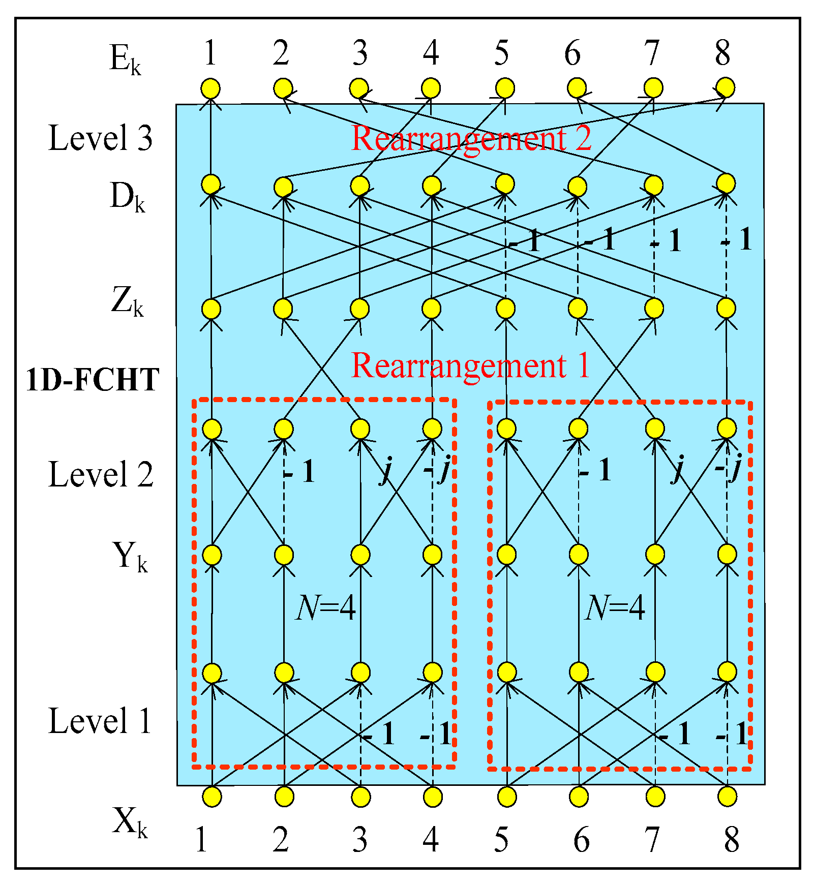
For N = 4 (respectively, n = 2), Equations (17)–(19) for i, u = 0,1,2,3 are transformed into:

$$\left[\begin{array}{c}\mathrm{s}(0)\\ \mathrm{s}(1)\\ \mathrm{s}(2)\\ \mathrm{s}(3)\end{array}\right]=\left[\begin{array}{cccc}1& 1& 1& 1\\ 1& -1& \mathrm{j}& -\mathrm{j}\\ 1& 1& -1& -1\\ 1& -1& -\mathrm{j}& \mathrm{j}\end{array}\right]\left[\begin{array}{c}\mathrm{x}(0)\\ \mathrm{x}(2)\\ \mathrm{x}(1)\\ \mathrm{x}(3)\end{array}\right]; \left[\begin{array}{c}\mathrm{x}(0)\\ \mathrm{x}(1)\\ \mathrm{x}(2)\\ \mathrm{x}(3)\end{array}\right]=\frac{1}{4}\left[\begin{array}{cccc}1& 1& 1& 1\\ 1& -1& -\mathrm{j}& \mathrm{j}\\ 1& 1& -1& -1\\ 1& -1& \mathrm{j}& -\mathrm{j}\end{array}\right]\left[\begin{array}{c}\mathrm{s}(0)\\ \mathrm{s}(2)\\ \mathrm{s}(1)\\ \mathrm{s}(3)\end{array}\right].$$

(20)

In this case, in accordance with Equation (20), for the calculation of the direct/inverse 1D-CHT are needed four basic “butterfly” operations, whose weight coefficients are, respectively, (+1,−1) for three of the “butterflies” and (+j,−j) for the fourth.

In Figure 3 is shown the calculation graph of the direct 3-level fast hierarchical 1D-CHT (n = 3) for N = 8, built in accordance with Figure 2.

The graph for the 1D-FCHT when N = 8 is created on the basis of Equation (20), to which are added four “butterfly” operations with weight coefficients (+1,−1) in the last, third level. In the result of the use of the frequency-ordered 1D-FCHT [14] is obtained the following system of equations, which represent the relations between the sequences of the input and output matrices, respectively X_k and E_k, for k = 1, 2, …, 8 and N = 8:

$$\begin{array}{l}{\mathrm{E}}_1={\mathrm{X}}_1+{\mathrm{X}}_2+{\mathrm{X}}_3+{\mathrm{X}}_4+{\mathrm{X}}_5+{\mathrm{X}}_6+{\mathrm{X}}_7+{\mathrm{X}}_8;\\ {\mathrm{E}}_2={\mathrm{X}}_1+{\mathrm{X}}_2+{\mathrm{X}}_3+{\mathrm{X}}_4-{\mathrm{X}}_5-{\mathrm{X}}_6-{\mathrm{X}}_7-{\mathrm{X}}_8;\\ {\mathrm{E}}_3={\mathrm{X}}_1-{\mathrm{X}}_3-{\mathrm{X}}_5+{\mathrm{X}}_7+\mathrm{j}({\mathrm{X}}_2-{\mathrm{X}}_4-{\mathrm{X}}_6+{\mathrm{X}}_8);\\ {\mathrm{E}}_4={\mathrm{X}}_1-{\mathrm{X}}_3+{\mathrm{X}}_5-{\mathrm{X}}_7+\mathrm{j}({\mathrm{X}}_2-{\mathrm{X}}_4+{\mathrm{X}}_6-{\mathrm{X}}_8);\end{array} \begin{array}{l}{\mathrm{E}}_5={\mathrm{X}}_1-{\mathrm{X}}_3+{\mathrm{X}}_5-{\mathrm{X}}_7-\mathrm{j}({\mathrm{X}}_2-{\mathrm{X}}_4+{\mathrm{X}}_6-{\mathrm{X}}_8);\\ {\mathrm{E}}_6={\mathrm{X}}_1-{\mathrm{X}}_3-{\mathrm{X}}_5+{\mathrm{X}}_7-\mathrm{j}({\mathrm{X}}_2-{\mathrm{X}}_4-{\mathrm{X}}_6+{\mathrm{X}}_8);\\ {\mathrm{E}}_7={\mathrm{X}}_1-{\mathrm{X}}_2+{\mathrm{X}}_3-{\mathrm{X}}_4-{\mathrm{X}}_5+{\mathrm{X}}_6-{\mathrm{X}}_7+{\mathrm{X}}_8;\\ {\mathrm{E}}_8={\mathrm{X}}_1-{\mathrm{X}}_2+{\mathrm{X}}_3-{\mathrm{X}}_4+{\mathrm{X}}_5-{\mathrm{X}}_6+{\mathrm{X}}_7-{\mathrm{X}}_8.\end{array}$$

(21)

Unlike Equation (14), part of the equations in the system above contain the complex variable $\mathrm{j}=\sqrt{-1}$, and they represent complex matrices (i.e., these are relations E₃, E₄, E₅ and E₆). The remaining four equations (E₁, E₂, E₇ and E₈) represent real matrices. The components of each complex matrix ${\mathrm{E}}_{\mathrm{k}}={\mathrm{A}}_{\mathrm{k}}+\mathrm{j}{\mathrm{B}}_{\mathrm{k}}$ (k = 3,4,5,6) are ${\mathrm{A}}_{\mathrm{k}}={\displaystyle \sum _{\mathrm{p}=1,3,5,7}{\mathsf{\alpha }}_{\mathrm{p}}{\mathrm{X}}_{\mathrm{p}}}$ and ${\mathrm{B}}_{\mathrm{k}}={\displaystyle \sum _{\mathrm{p}=2,4,6,8}{\mathsf{\beta }}_{\mathrm{p}}{\mathrm{X}}_{\mathrm{p}}}$; α_p and β_p are sign functions with values of +1 or −1, defined by Equation (21). The elements e(i,m.k) of the complex matrix E_k are defined as follows:

$$\mathrm{e}(\mathrm{i},\mathrm{m},\mathrm{k})={\mathrm{e}(\mathrm{i},\mathrm{m},\mathrm{k})}_{\mathrm{Re}}+\mathrm{j}{\mathrm{e}(\mathrm{i},\mathrm{m},\mathrm{k})}_{\mathrm{Im}}={ \mathrm{M}}_{\mathrm{k}}(\mathrm{i},\mathrm{m}){\mathrm{e}}^{\mathrm{j}{\mathrm{\Phi }}_{\mathrm{k}}(\mathrm{i},\mathrm{m})},$$

(22)

where ${\mathrm{M}}_{\mathrm{k}}(\mathrm{i},\mathrm{m})=\sqrt{\mathrm{e}(\mathrm{i},\mathrm{m},{\mathrm{k})}_{\mathrm{Re}}^2 +\mathrm{e}(\mathrm{i},\mathrm{m},{\mathrm{k})}_{\mathrm{Im}}^2 }$ is a module; and ${\mathrm{\Phi }}_{\mathrm{k}}(\mathrm{i},\mathrm{m})=\mathrm{arctg}[\mathrm{e}(\mathrm{i},\mathrm{m},{\mathrm{k})}_{\mathrm{Im}}/\mathrm{e}(\mathrm{i},\mathrm{m},{\mathrm{k})}_{\mathrm{Re}}]$, a phase of the element e(i,m,k).

The matrix Φ_k permits the phase modification of its elements, which could be used (for example) for the resistant digital watermarking of multidimensional signals and images [14].

In Appendix A.2 is presented in detail the factorization of the matrix for an n-level hierarchical frequency-ordered 1D-FCHT, based on the “butterfly” operation (Equation (20)) used for the 1D-CHT execution, if N = 4.

4. Hierarchical Cubical Tensor Decomposition through the 3D-FWHT

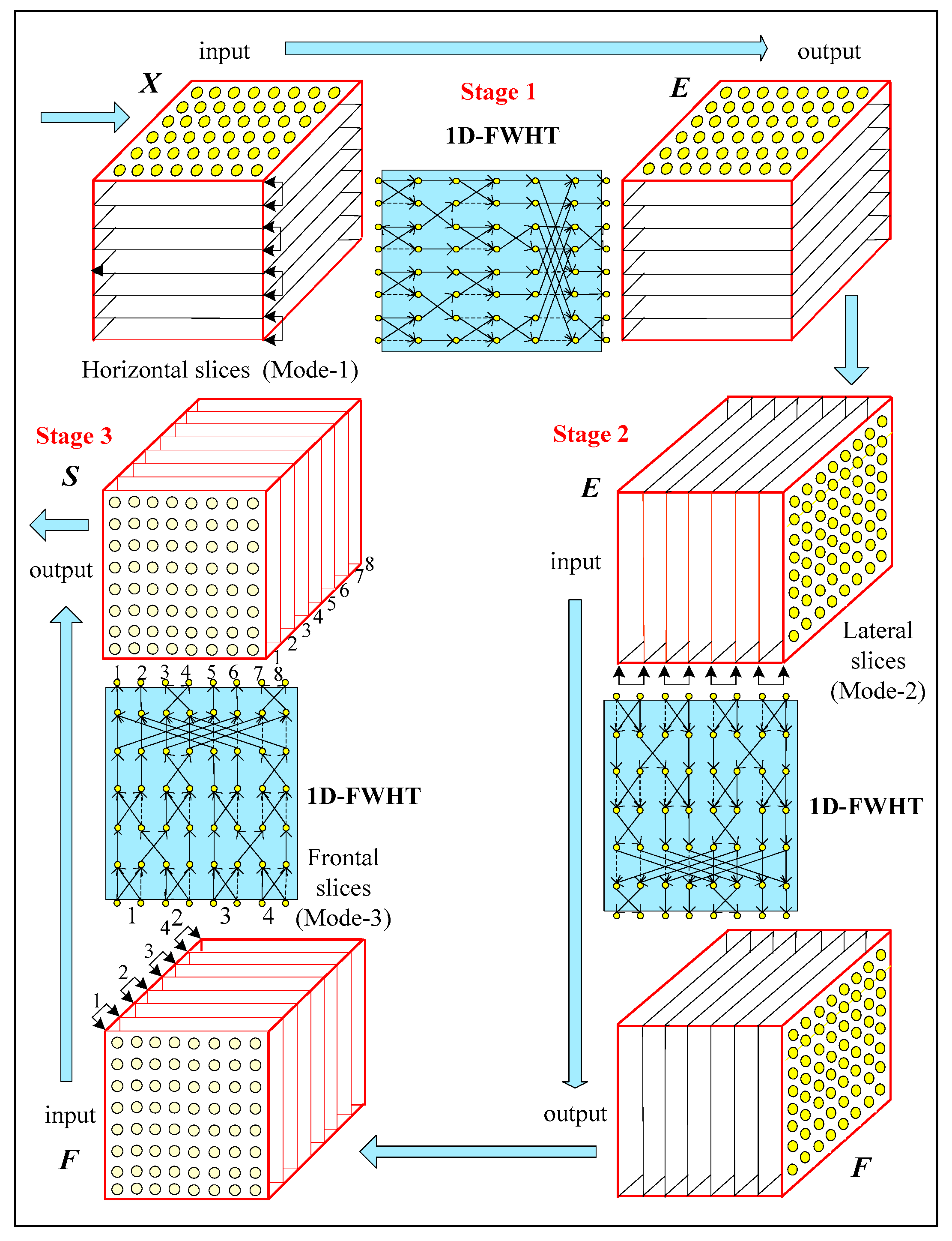
At first, here is described the decomposition of the cubical tensor X of size 8 × 8 × 8. In this case, the decomposition could be represented in the simplified form shown in Figure 4.

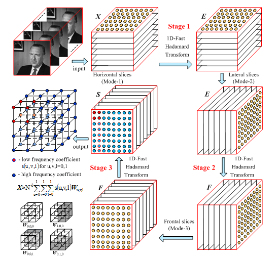
The decomposition based on the 3D-FWHT comprises three stages. In the first stage, the tensor is divided into horizontal slices (mode-1), after which, on each couple of matrices, is applied the 1D-FWHT, and from the so obtained eight slices is restored the tensor E. In a similar way are executed the operations in the second and third stages. Unlike in the first, in the second stage, the input tensor E is divided into eight lateral slices (mode-2). After their transform through the 1D-FWHT, from the obtained eight slices is restored the tensor F. In the third stage, the tensor F is divided into eight frontal slices (mode-3), from which, after the 1D-FWHT, is obtained the spectrum tensor S with elements $\mathrm{s}(\mathrm{u},\mathrm{v},\mathrm{l})$. From this tensor, after the reverse execution of the three stages of the inverse 1D-FWHT, is restored the initial tensor X with elements x(i,j,k). 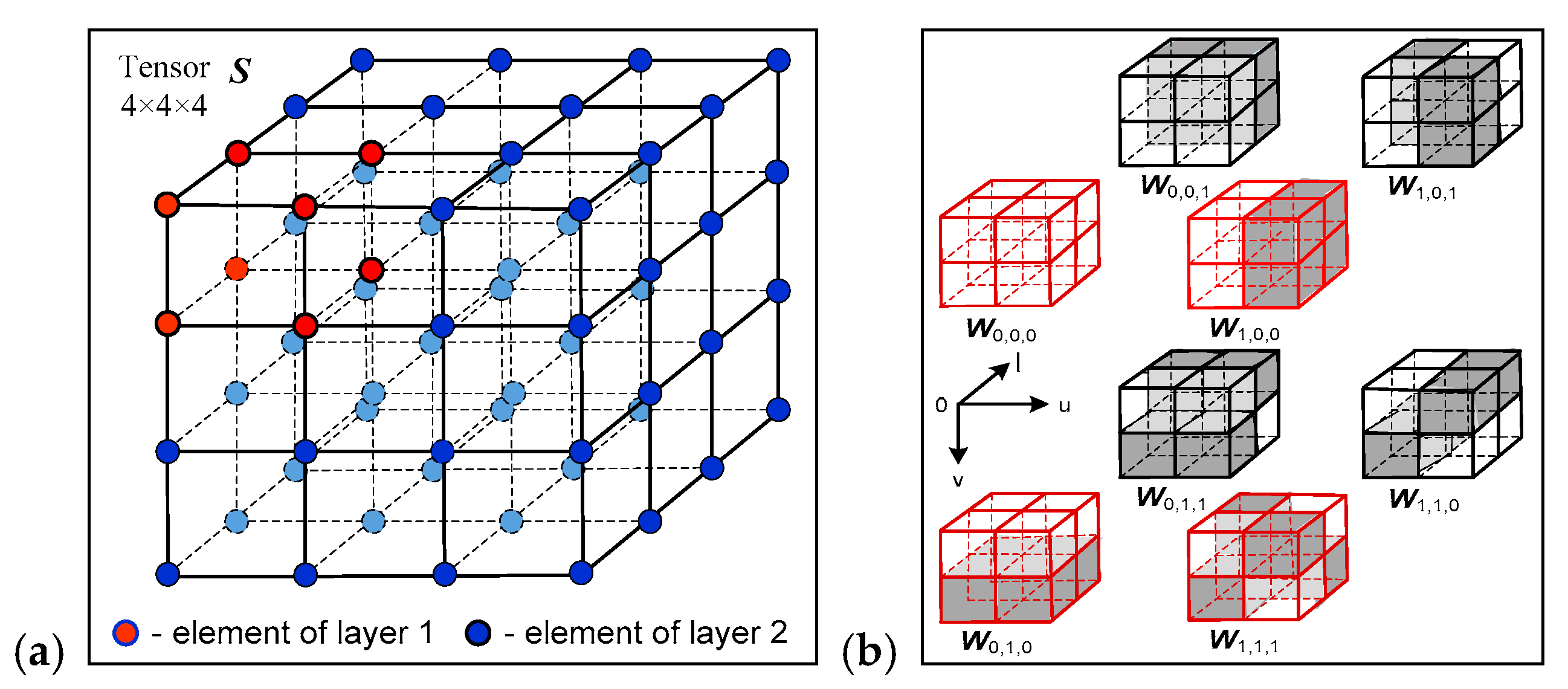In the result of the decomposition, it is represented as a sum of weighted “basic” tensors ${\mathit{W}}_{u,v,l}$ of size 8 × 8 × 8 with elements wal(u,v,l), which are 3D Walsh functions:

$$\mathit{X}=(1/512)[\mathrm{s}(0,0,0){\mathit{W}}_{0,0,0}+\mathrm{s}(1,0,0){\mathit{W}}_{1,0,0}+\dots +\mathrm{s}(7,7,7){\mathit{W}}_{7,7,7}]=(1/8^3){\displaystyle \sum _{\mathrm{u}=0}^7{\displaystyle \sum _{\mathrm{v}=0}^7{\displaystyle \sum _{\mathrm{l}=0}^7\mathrm{s}(\mathrm{u},\mathrm{v},\mathrm{l}){\mathit{W}}_{\mathrm{u},\mathrm{v},\mathrm{l}} }}}.$$

(23)

The 3D functions wal(u,v,l) are divisible [16,17], and they could be represented as the product of three 1D Walsh functions: wal(u).wal(v).wal(l). The coefficients s(u,v,l) for u = 0,1, v = 0,1 and l = 0,1 in the first layer correspond to the lowest spatial frequencies of the spectrum tensor, S. In Figure 5a is shown an example for a spectrum tensor S of size 4 × 4 × 4, and in Figure 5b, the 8 “basic” tensors, which correspond to coefficients s(u,v,l) from the initial layer of the tensor S [18].

The 3D-FWHT algorithm, shown in Figure 4, could be generalized for the case when N = 2ⁿ by creating an extended n-level computational graph in correspondence with the transform matrix factorization explained in Appendix A.1. The number of stages needed for the execution of the 1D-FWHT (in accordance with Figure 4) is three, not only for N = 8 but also for the higher values of N = 16, 32,…

In the general case, the spectrum coefficients s(u,v,l) are calculated through the direct 3D-WHT, in accordance with the relation [12,18]:

$$\mathrm{s}(\mathrm{u},\mathrm{v},\mathrm{l})={\displaystyle \sum _{\mathrm{i}=0}^{\mathrm{N}-1}{\displaystyle \sum _{\mathrm{k}=0}^{\mathrm{N}-1}{\displaystyle \sum _{\mathrm{l}=0}^{\mathrm{N}-1} \mathrm{x}(\mathrm{i},\mathrm{j},\mathrm{k} )\mathrm{w}\mathrm{a}\mathrm{l}(\mathrm{i},\mathrm{u})\mathrm{w}\mathrm{a}\mathrm{l}(\mathrm{j},\mathrm{v})\mathrm{w}\mathrm{a}\mathrm{l}(\mathrm{k},\mathrm{l})}}} \mathrm{for} \mathrm{u},\mathrm{v},\mathrm{l} = 0,1,\dots ,\mathrm{N}-1.$$

(24)

The 3D inverse WHT (3D-IWHT) is defined by the relation:

$$\mathrm{x}(\mathrm{i},\mathrm{m},\mathrm{k})=\frac{1}{{\mathrm{N}}^3}{\displaystyle \sum _{\mathrm{u}=0}^{\mathrm{N}-1}{\displaystyle \sum _{\mathrm{v}=0}^{\mathrm{N}-1}{\displaystyle \sum _{\mathrm{l}=0}^{\mathrm{N}-1}\mathrm{s}(\mathrm{u},\mathrm{v},\mathrm{l})\mathrm{w}\mathrm{a}\mathrm{l}(\mathrm{i},\mathrm{u})\mathrm{w}\mathrm{a}\mathrm{l}(\mathrm{m},\mathrm{v})\mathrm{w}\mathrm{a}\mathrm{l}(\mathrm{k},\mathrm{l})}}} \mathrm{for}\mathrm{i},\mathrm{m},\mathrm{k} = 0,1,\dots ,\mathrm{N}-1.$$

(25)

Here, the discrete one-dimensional Walsh-Hadamard (WH) functions of N^th order wal(i,u), wal(m,v), wal(k,l) for i,m,k = 0,1, …,N−1, are defined by the following relations:

$$\mathrm{wal}(\mathrm{i},\mathrm{u})={(-1)}^{{\displaystyle \sum _{\mathrm{r}=0}^{\mathrm{n}-1}{\mathrm{q}}_{\mathrm{r}}(\mathrm{i}){\mathrm{u}}_{\mathrm{r}}}}, \mathrm{wal}(\mathrm{m},\mathrm{v})={(-1)}^{{\displaystyle \sum _{\mathrm{r}=0}^{\mathrm{n}-1}{\mathrm{q}}_{\mathrm{r}}(\mathrm{m}){\mathrm{v}}_{\mathrm{r}}}}, \mathrm{wal}(\mathrm{k},\mathrm{l})={(-1)}^{{\displaystyle \sum _{\mathrm{r}=0}^{\mathrm{n}-1}{\mathrm{q}}_{\mathrm{r}}(\mathrm{k}){\mathrm{l}}_{\mathrm{r}}}},$$

(26)

where ${\mathrm{q}}_{\mathrm{r}}(\mathrm{i}),{\mathrm{q}}_{\mathrm{r}}(\mathrm{m}),{\mathrm{q}}_{\mathrm{r}}(\mathrm{k})$ and ${\mathrm{u}}_{\mathrm{r}},{\mathrm{v}}_{\mathrm{r}},{\mathrm{l}}_{\mathrm{r}}$ are defined by analogy with Equation (2) after converting the decimal numbers i, m, k and u, v, l into binary, respectively: $\mathrm{i}={\displaystyle \sum _{\mathrm{r}=0}^{\mathrm{n}-1}{\mathrm{i}}_{\mathrm{r}}{2}^{\mathrm{r}}},$$\mathrm{m}={\displaystyle \sum _{\mathrm{r}=0}^{\mathrm{n}-1}{\mathrm{m}}_{\mathrm{r}}{2}^{\mathrm{r}}},$$\mathrm{k}={\displaystyle \sum _{\mathrm{r}=0}^{\mathrm{n}-1}{\mathrm{k}}_{\mathrm{r}}{2}^{\mathrm{r}}}$ and $\mathrm{v}={\displaystyle \sum _{\mathrm{r}=0}^{\mathrm{n}-1}{\mathrm{v}}_{\mathrm{r}}{2}^{\mathrm{r}}},$$\mathrm{u}={\displaystyle \sum _{\mathrm{r}=0}^{\mathrm{n}-1}{\mathrm{u}}_{\mathrm{r}}{2}^{\mathrm{r}}},$$\mathrm{l}={\displaystyle \sum _{\mathrm{r}=0}^{\mathrm{n}-1}{\mathrm{l}}_{\mathrm{r}}{2}^{\mathrm{r}}}$ for n = log₂N.

Each 3^d-order tensor X of size N × N × N could be calculated by using the weighted sum of the N³ 3D WH functions represented through tensors ${\mathit{W}}_{\mathit{u}\mathit{,}\mathit{v}\mathit{,}\mathit{l}}$, each of size N × N × N:

$$\mathit{X}=(1/{\mathrm{N}}^3)[\mathrm{s}(0,0,0){\mathit{W}}_{0,0,0}+\mathrm{s}(1,0,0){\mathit{W}}_{1,0,0}+\dots +\mathrm{s}(\mathrm{N}-1,\mathrm{N}-1,\mathrm{N}-1){\mathit{W}}_{\mathrm{N}-1,\mathrm{N}-1,\mathrm{N}-1}]=(1/{\mathrm{N}}^3){\displaystyle \sum _{\mathrm{u}=0}^{\mathrm{N}-1}{\displaystyle \sum _{\mathrm{v}=0}^{\mathrm{N}-1}{\displaystyle \sum _{\mathrm{l}=0}^{\mathrm{N}-1}\mathrm{s}(\mathrm{u},\mathrm{v},\mathrm{l} ) {\mathit{W}}_{\mathrm{u},\mathrm{v},\mathrm{l}} }}.}$$

(27)

Each “basic” tensor ${\mathit{W}}_{\mathit{u}\mathit{,}\mathit{v}\mathit{,}\mathit{l}}$ with frequency (u,v,l) could be represented through the outer product of the vectors ${\overrightarrow{\mathrm{w}}}_{\mathrm{u}},{\overrightarrow{\mathrm{w}}}_{\mathrm{v}},{\overrightarrow{\mathrm{w}}}_{\mathrm{l}}:$

$${\mathit{W}}_{\mathit{u}\mathit{,}\mathit{v}\mathit{,}\mathit{l}}={\overrightarrow{\mathrm{w}}}_{\mathrm{u}}\circ {\overrightarrow{\mathrm{w}}}_{\mathrm{v}}\circ {\overrightarrow{\mathrm{w}}}_{\mathrm{l}},$$

(28)

where the vectors, which represent the tensor ${\mathit{W}}_{\mathit{u},\mathit{v},\mathit{l}}$, are defined by the relations below:

$${\overrightarrow{\mathrm{w}}}_{\mathrm{u}}={[{(-1)}^{{\displaystyle \sum _{\mathrm{r}=0}^{\mathrm{n}-1}{\mathrm{q}}_{\mathrm{r}}(0){\mathrm{u}}_{\mathrm{r}}}},{(-1)}^{{\displaystyle \sum _{\mathrm{r}=0}^{\mathrm{n}-1}{\mathrm{q}}_{\mathrm{r}}(1){\mathrm{u}}_{\mathrm{r}}}},\dots ,{(-1)}^{{\displaystyle \sum _{\mathrm{r}=0}^{\mathrm{n}-1}{\mathrm{q}}_{\mathrm{r}}(\mathrm{N}-1){\mathrm{u}}_{\mathrm{r}}}}]}^{\mathrm{T}};$$

(29)

$${\overrightarrow{\mathrm{w}}}_{\mathrm{v}}={[{(-1)}^{{\displaystyle \sum _{\mathrm{r}=0}^{\mathrm{n}-1}{\mathrm{q}}_{\mathrm{r}}(0){\mathrm{v}}_{\mathrm{r}}}},{(-1)}^{{\displaystyle \sum _{\mathrm{r}=0}^{\mathrm{n}-1}{\mathrm{q}}_{\mathrm{r}}(1){\mathrm{v}}_{\mathrm{r}}}},\dots ,{(-1)}^{{\displaystyle \sum _{\mathrm{r}=0}^{\mathrm{n}-1}{\mathrm{q}}_{\mathrm{r}}(\mathrm{N}-1){\mathrm{v}}_{\mathrm{r}}}}]}^{\mathrm{T}};$$

(30)

$${\overrightarrow{\mathrm{w}}}_{\mathrm{l}}={[{(-1)}^{{\displaystyle \sum _{\mathrm{r}=0}^{\mathrm{n}-1}{\mathrm{q}}_{\mathrm{r}}(0){\mathrm{l}}_{\mathrm{r}}}},{(-1)}^{{\displaystyle \sum _{\mathrm{r}=0}^{\mathrm{n}-1}{\mathrm{q}}_{\mathrm{r}}(1){\mathrm{l}}_{\mathrm{r}}}},\dots ,{(-1)}^{{\displaystyle \sum _{\mathrm{r}=0}^{\mathrm{n}-1}{\mathrm{q}}_{\mathrm{r}}(\mathrm{N}-1){\mathrm{l}}_{\mathrm{r}}}}]}^{\mathrm{T}}.$$

(31)

Then, the tensor decomposition based on the 3D-WHT, is defined by the relation:

$$\mathit{X}=(1/{\mathrm{N}}^3){\displaystyle \sum _{\mathrm{u}=0}^{\mathrm{N}-1}{\displaystyle \sum _{\mathrm{v}=0}^{\mathrm{N}-1}{\displaystyle \sum _{\mathrm{l}=0}^{\mathrm{N}-1}\mathrm{s}(\mathrm{u},\mathrm{v},\mathrm{l})[{\overrightarrow{\mathrm{w}}}_{\mathrm{u}}\circ {\overrightarrow{\mathrm{w}}}_{\mathrm{v}}\circ {\overrightarrow{\mathrm{w}}}_{\mathrm{l}}].}}}.$$

(32)

As follows from the relations in Equations (25) and (32), the 3D-WHT is reversible, i.e., X could be restored from the tensor S through the 3D-IWTH. The decomposition in Equation (32) of the tensor X of size N × N × N corresponds to the Tucker decomposition [1,3,5]:

$$\mathit{X}={\displaystyle \sum _{{\mathrm{r}}_1=1}^{{\mathrm{R}}_1}{\displaystyle \sum _{{\mathrm{r}}_2=1}^{{\mathrm{R}}_2}{\displaystyle \sum _{{\mathrm{r}}_3=1}^{{\mathrm{R}}_3}{\mathrm{g}}_{{\mathrm{r}}_1,{\mathrm{r}}_2,{\mathrm{r}}_3}({\overrightarrow{\mathrm{a}}}_{{\mathrm{r}}_1}\circ {\overrightarrow{\mathrm{b}}}_{{\mathrm{r}}_2}\circ {\overrightarrow{\mathrm{c}}}_{{\mathrm{r}}_3} )}}}.$$

(33)

Here, ${\mathrm{g}}_{{\mathrm{r}}_1,{\mathrm{r}}_2,{\mathrm{r}}_3}$ are the entries of the core tensor G of size R₁ × R₂ × R₃, and R₁, R₂, R₃, the multilinear rank of the tensor X. For the case, when it is a cube of size N × N × N, the tensor G is diagonal and of size R×R×R; g_r (for r = 1,2, …,R) are its eigen values, and ${\overrightarrow{\mathrm{a}}}_{{\mathrm{r}}_1},{\overrightarrow{\mathrm{b}}}_{{\mathrm{r}}_2},{\overrightarrow{\mathrm{c}}}_{{\mathrm{r}}_3}$, the eigen vectors. In this case, the Tucker decomposition is transformed into CPD [1], and is represented by the relation below:

$$\mathit{X}={\displaystyle \sum _{\mathrm{r}=1}^{\mathrm{R}}{\mathrm{g}}_{\mathrm{r}} ({\overrightarrow{\mathrm{a}}}_{\mathrm{r}}\circ {\overrightarrow{\mathrm{b}}}_{\mathrm{r}}\circ {\overrightarrow{\mathrm{c}}}_{\mathrm{r}})}.$$

(34)

Here, R is the rank of the tensor X, whose value is limited in the range $\mathrm{N}\le \mathrm{R}\le {\mathrm{N}}^2$ [19]. The difference between the decompositions, represented by Equations (33) and (32), is in the numbers of their components; in the first case, it is ≤N², and in the second, it is ≤N³. This shows the higher energy concentration in the first components of the H-Tucker decomposition (respectively, CPD) compared to that of the 3D-WHT.

5. Hierarchical Cubical Tensor Decomposition through the 3D-FCHT

The comparison of the relations in Equations (14), (15) and (21) shows that the 1D-FWHT and 1D-FCHT are executed in accordance with algorithms with similar structure (Figure 2 and Figure 3). From this, it follows that for the decomposition of the tensor X of size 8 × 8 × 8 through 3D-FCHT could be used the three-stage scheme shown in Figure 4. The difference is that in the three decomposition stages, the 1D-FWHT algorithm from Figure 2 must be replaced by this for the 1D-FCHT, shown in Figure 3. After the triple execution of the algorithm is obtained the spectrum tensor S (shown on Figure 4) with elements $\mathrm{s}(\mathrm{u},\mathrm{v},\mathrm{l}),$ half of which are complex. The 3D-FCHT algorithm, shown in Figure 3, could be generalized for the case when N = 2ⁿ by creating an extended computational graph of n levels. The number of stages needed for the execution of the 1D-FCHT by analogy with the 3D-FWHT is also three (not for N = 8 only but also for the next values of N = 16, 32, …).

In the general case, the decomposition of the tensor X of size N × N × N in accordance with Equation (27) is represented as the sum of the weighted “basic” tensors:

$$\mathit{X}=(1/{\mathrm{N}}^3){\displaystyle \sum _{\mathrm{u}=0}^{\mathrm{N}-1}{\displaystyle \sum _{\mathrm{v}=0}^{\mathrm{N}-1}{\displaystyle \sum _{\mathrm{l}=0}^{\mathrm{N}-1}\mathrm{s}(\mathrm{u},\mathrm{v},\mathrm{l}){\mathit{C}}_{\mathrm{u},\mathrm{v},\mathrm{l}}}}}=(1/{\mathrm{N}}^3){\displaystyle \sum _{\mathrm{u}=0}^{\mathrm{N}-1}{\displaystyle \sum _{\mathrm{v}=0}^{\mathrm{N}-1}{\displaystyle \sum _{\mathrm{l}=0}^{\mathrm{N}-1}\mathrm{s}(\mathrm{u},\mathrm{v},\mathrm{l})[{\overrightarrow{\mathrm{c}}}_{\mathrm{u}}\circ {\overrightarrow{\mathrm{c}}}_{\mathrm{v}}\circ {\overrightarrow{\mathrm{c}}}_{\mathrm{l}}}]}},$$

(35)

where ${\mathit{C}}_{\mathit{u}\mathit{,}\mathit{v}\mathit{,}\mathit{l}}={\overrightarrow{\mathrm{c}}}_{\mathrm{u}}\circ {\overrightarrow{\mathrm{c}}}_{\mathrm{v}}\circ {\overrightarrow{\mathrm{c}}}_{\mathrm{l}}.$ The vectors which define the tensor ${\mathit{C}}_{\mathit{u}\mathit{,}\mathit{v}\mathit{,}\mathit{l}}$ are defined by the relations below:

$${\overrightarrow{\mathrm{c}}}_{\mathrm{u}}={[\mathrm{h}(0,\mathrm{u}),{\mathrm{j}}^{\mathrm{u}}\mathrm{h}(1,\mathrm{u}),\dots ,{\mathrm{j}}^{\mathrm{i}\mathrm{u}}\mathrm{h}(\mathrm{i},\mathrm{u}),\dots ,{\mathrm{j}}^{(\mathrm{N}-1)\mathrm{u}}\mathrm{h}(\mathrm{N}-1,\mathrm{u})]}^{\mathrm{T}};$$

(36)

$${\overrightarrow{\mathrm{c}}}_{\mathrm{v}}={[\mathrm{h}(0,\mathrm{v}),{\mathrm{j}}^{\mathrm{v}}\mathrm{h}(1,\mathrm{v}),\dots ,{\mathrm{j}}^{\mathrm{m}\mathrm{v}}\mathrm{h}(\mathrm{m},\mathrm{v}),\dots ,{\mathrm{j}}^{(\mathrm{N}-1)\mathrm{v}}\mathrm{h}(\mathrm{N}-1,\mathrm{v})]}^{\mathrm{T}};$$

(37)

$${\overrightarrow{\mathrm{c}}}_{\mathrm{l}}={[\mathrm{h}(0,\mathrm{l}),{\mathrm{j}}^{\mathrm{l}}\mathrm{h}(1,\mathrm{l}),\dots ,{\mathrm{j}}^{\mathrm{k}\mathrm{l}}\mathrm{h}(\mathrm{k},\mathrm{l}),\dots ,{\mathrm{j}}^{(\mathrm{N}-1)\mathrm{l}}\mathrm{h}(\mathrm{N}-1,\mathrm{l})]}^{\mathrm{T}}.$$

(38)

In the above relations, the sign functions h(i,u), h(m,v) and h(k,l) for i,m,k = 0, 1, …, N−1 are defined by Equation (19). The spectrum coefficients s(u,v,l) in Equation (35) are calculated through the direct 3D-CHT, in accordance with the relation:

$$\mathrm{s}(\mathrm{u},\mathrm{v},\mathrm{l})={\displaystyle \sum _{\mathrm{i}=0}^{\mathrm{N}-1}{\displaystyle \sum _{\mathrm{k}=0}^{\mathrm{N}-1}{\displaystyle \sum _{\mathrm{l}=0}^{\mathrm{N}-1}\mathrm{x}(\mathrm{i},\mathrm{m},\mathrm{k}){\mathrm{j}}^{(\mathrm{i}\mathrm{u}+\mathrm{m}\mathrm{v}+\mathrm{k}\mathrm{l})}\mathrm{h}(\mathrm{i},\mathrm{u})\mathrm{h}(\mathrm{m},\mathrm{v})\mathrm{h}(\mathrm{k},\mathrm{l})}}} \mathrm{for} \mathrm{u},\mathrm{v},\mathrm{l}=0,1,\dots ,\mathrm{N}-1.$$

(39)

The 3D inverse CHT (3D-ICHT) is defined as follows:

$$\mathrm{x}(\mathrm{i},\mathrm{m},\mathrm{k})=(1/{\mathrm{N}}^3){\displaystyle \sum _{\mathrm{i}=0}^{\mathrm{N}-1}{\displaystyle \sum _{\mathrm{k}=0}^{\mathrm{N}-1}{\displaystyle \sum _{\mathrm{l}=0}^{\mathrm{N}-1} \mathrm{s}(\mathrm{u},\mathrm{v},\mathrm{l}){\mathrm{j}}^{-(\mathrm{i}\mathrm{u}+\mathrm{m}\mathrm{v}+\mathrm{k}\mathrm{l})}\mathrm{h}(\mathrm{i},\mathrm{u})\mathrm{h}(\mathrm{m},\mathrm{v})\mathrm{h}(\mathrm{k},\mathrm{l})}}} \mathrm{for} \mathrm{i},\mathrm{m},\mathrm{k}=0,1,\dots ,\mathrm{N}-1.$$

(40)

6. Comparative CC Evaluation for the 3D-FWHT and 3D-FCWHT Algorithm

In this section is evaluated the CC of the decomposition algorithms for a tensor of size N × N × N, when N = 2ⁿ.

6.1. CC of the Algorithm Based on the Real Orthogonal Transform, 3D-FWHT

The number of additions, A_W(1), needed for the execution of the 1D-WHT based on the “butterfly” operation for all N² elements of a couple of matrices, both of size N × N, is:

$${\mathrm{A}}_{1\mathrm{H}}(1)=2{\mathrm{N}}^2.$$

(41)

For all N/2 couples of matrices in one stage of the hierarchical 3D-FWHT of n levels, this number is:

$${\mathrm{A}}_{1\mathrm{H}}(\mathrm{n})=(\mathrm{N}/2)2{\mathrm{N}}^2{\lg }_2\mathrm{N}=2^{3\mathrm{n}}\mathrm{n}.$$

(42)

Then, for the three stages of the hierarchical 3D-FWHT is obtained:

$${\mathrm{A}}_{3\mathrm{H}}(\mathrm{n})=3\times 2^{3\mathrm{n}}\mathrm{n}.$$

(43)

The needed number of multiplications for the execution of the direct 3D-FWHT is M_3H(n) = 0. Then, the CC of the 3D-FWHT evaluated through the total number of operations O_3H(n) is defined by the relation:

$${\mathrm{O}}_{3\mathrm{H}}(\mathrm{n})={\mathrm{A}}_{3\mathrm{H}}(\mathrm{n})+{\mathrm{M}}_{3\mathrm{H}}(\mathrm{n})=3\times 2^{3\mathrm{n}}\mathrm{n}.$$

(44)

6.2. CC of the Algorithm Based on the Complex Orthogonal Transform, 3D-FCHT

The number of additions for all N² elements of N/2 couples of matrices of size N × N in one stage of the hierarchical n-level 1D-FCHT is:

$${\mathrm{A}}_{1\mathrm{C}}(\mathrm{n})={\mathrm{N}}^2\{(3/2)\mathrm{N}+(\mathrm{n}-2)[(\mathrm{N}/4)+2(3\mathrm{N}/4)]\}=2^{3\mathrm{n}+1}(0.875\mathrm{n}-1).$$

(45)

In the relation above is taken into account that in the first level of the 1D-FCHT are added N real numbers; in the second level, there are N/2 real numbers, and in the remaining (n-2) levels, N/4 real and 3N/4 complex numbers. Additionally, the summarizing of two complex numbers is executed as a sum of two couples of real numbers.

Then, for the three stages of the 3D Fast CHT (3D-FCHT), the number of needed additions is:

$${\mathrm{A}}_{3\mathrm{C}}(\mathrm{n})=3\times 2^{3\mathrm{n}}\mathrm{n}=6\times 2^{3\mathrm{n}}(0.875\mathrm{n}-1).$$

(46)

The number of complex multiplications needed for the direct 3D-FCHT is M_3C(n) = 0 (the multiplication of j by a real number is not an arithmetical operation but only needs larger memory in which to save the so obtained complex number). Then, the CC of the 3D-FCHT, evaluated on the basis of the global number of needed operations O_3C(n), is defined by the relation:

$${\mathrm{O}}_{3\mathrm{C}}(\mathrm{n})={\mathrm{A}}_{3\mathrm{C}}(\mathrm{n})+{\mathrm{M}}_{3\mathrm{C}}(\mathrm{n})=6\times 2^{3\mathrm{n}}(0.875\mathrm{n}-1).$$

(47)

6.3. CC of the Algorithm Based on the Complex Orthogonal Transform, 3D-DFT

The divisibility of the 3D fast Fourier transform (3D-DFT) permits the tensor decomposition to be executed through applying the 1D-DFT on all fibers (vectors) obtained in the result of the tensor transform, called vectorization [1,3]. The vectors are oriented in three directions: x (mode-1), y (mode-2) and z (mode-3). The calculation of the 1D-DFT is based on the Cooley-Tukey algorithm for Fast Fourier Transform (FFT) [15]. In the result of the calculation of the radix-2 FFT for an N-dimensional vector, the number of operations (respectively, CC) is reduced from N² to Nlog₂N = Nn. Then, the CC of the 3D-FFT is O(N_clog₂N_c), where N_c = N₁ × N₂ × N₃. In the case that N₁ = N₂ = N₃ = N = 2ⁿ, for a tensor of N³ voxels, the number of the complex additions is ${\mathrm{A}}_{3\mathrm{F}}(\mathrm{n})={\mathrm{N}}^3{\log }_2{\mathrm{N}}^3=3{\mathrm{N}}^3\mathrm{n}$, and that of the complex multiplications, ${\mathrm{M}}_{3\mathrm{F}}(\mathrm{n})={(\mathrm{N}/2)}^3{\log }_2{\mathrm{N}}^3=(3/8){\mathrm{N}}^3\mathrm{n}$ [20]. The multiplication of two complex numbers is equivalent to four multiplications of real numbers, and one complex addition, to two additions of real numbers. Then, for the CC of the 3D-FFT is obtained:

$${\mathrm{O}}_{3\mathrm{F}}(\mathrm{n})={\mathrm{A}}_{3\mathrm{F}}(\mathrm{n})+{\mathrm{M}}_{3\mathrm{F}}(\mathrm{n})=6.75{\mathrm{N}}^3\mathrm{n}+0.75{\mathrm{N}}^3\mathrm{n}=7.5\times 2^{3\mathrm{n}}\mathrm{n}.$$

(48)

6.4. CC of the Algorithm Based on the 3D Discrete Wavelet Transform, 3D-DWT and H-Tucker

The global number of additions and multiplications needed to calculate the cubical tensor of size N × N × N through the 3D Discrete Wavelet Transform (3D-DWT) of n levels with orthogonal filters (3, 5), are correspondingly [20]:

$${\mathrm{A}}_{3\mathrm{W}\mathrm{T}}(\mathrm{n})=18{\mathrm{N}}^3{\displaystyle {\sum }_{\mathrm{p}=0}^{\mathrm{n}-1}{8}^{-\mathrm{p}}}=20.57{(2}^{3\mathrm{n}}-1) \mathrm{and} {\mathrm{M}}_{3\mathrm{WT}}(\mathrm{n})=24{\mathrm{N}}^3{\displaystyle {\sum }_{\mathrm{p}=0}^{\mathrm{n}-1}{8}^{-\mathrm{p}}}=27.43(2^{3\mathrm{n}}-1).$$

(49)

Then, the CC of the 3D-DWT is:

$${\mathrm{O}}_{3\mathrm{W}\mathrm{T}}(\mathrm{n})={\mathrm{A}}_{3\mathrm{W}\mathrm{T}}(\mathrm{n})+{\mathrm{M}}_{3\mathrm{W}\mathrm{T}}(\mathrm{n})\approx 48\times 2^{3\mathrm{n}}\mathrm{n}.$$

(50)

The H-Tucker decomposition [5] of the cubical tensor of minimum rank R = 2ⁿ (as defined in [19]), size N = 2ⁿ and order d = 3 requires O_HT (3 × 2³ⁿ + 2 × 2⁴ⁿ) operations. For the TT-decomposition [4], the CC for the same tensor is O_TT (3 × 2⁴ⁿ), i.e., it is approximately 1.5 times higher than that for the H-Tucker. This is why the H-Tucker transform was selected for the CC comparison with the analyzed 3D deterministic orthogonal transforms.

6.5. CC of 3D-FWHT and 3D-FCHT, Compared to 3D-FFT, 3D-DWT and H-Tucker

The relative acceleration $\mathsf{\psi }(\mathrm{n})$ of the calculations needed for the execution of the 3D-FWHT, 3D-FCHT and 3D-FFT compared to that of the 3D-DWT and H-Tucker is given in detail below:

3D-FWHT, 3D-FCHT and 3D-FFT compared to 3D-DWT:

$${\mathsf{\psi }}_1(\mathrm{n})={\mathrm{O}}_{3\mathrm{W}\mathrm{T}}(\mathrm{n})/{\mathrm{O}}_{3\mathrm{H}}(\mathrm{n})=(48\times 2^{3\mathrm{n}})/(3\times 2^{3\mathrm{n}}\mathrm{n})\approx 16/\mathrm{n};$$

(51)

$${\mathsf{\psi }}_3(\mathrm{n})={\mathrm{O}}_{3\mathrm{W}\mathrm{T}}(\mathrm{n})/{\mathrm{O}}_{3\mathrm{C}}(\mathrm{n})=(48 \times 2^{3\mathrm{n}})/[6\times 2^{3\mathrm{n}}(0.875\mathrm{n}-1)]\approx 8/(0.87\mathrm{n}-1);$$

(52)

$${\mathsf{\psi }}_5(\mathrm{n})={\mathrm{O}}_{3\mathrm{W}\mathrm{T}}(\mathrm{n})/{\mathrm{O}}_{3\mathrm{F}}(\mathrm{n})=(48\times 2^{3\mathrm{n}})/(7.5\times 2^{3\mathrm{n}}\mathrm{n})\approx 6.4/\mathrm{n}.$$

(53)

3D-FWHT, 3D-FCHT and 3D-FFT compared to H-Tucker:

$${\mathsf{\psi }}_2(\mathrm{n})={\mathrm{O}}_{\mathrm{H}\mathrm{T}}(\mathrm{n})/{\mathrm{O}}_{3\mathrm{H}}(\mathrm{n})=2^{3\mathrm{n}}(2^{\mathrm{n}+1}+3)/(3\times 2^{3\mathrm{n}}\mathrm{n})\approx 0.66\times (2^{\mathrm{n}}/\mathrm{n});$$

(54)

$${\mathsf{\psi }}_4(\mathrm{n})={\mathrm{O}}_{\mathrm{H}\mathrm{T}}(\mathrm{n})/{\mathrm{O}}_{3\mathrm{C}}(\mathrm{n})=2^{3\mathrm{n}}(2^{\mathrm{n}+1}+3)/[6\times 2^{3\mathrm{n}}(0.875\mathrm{n}-1)]\approx (0.33\times 2^{\mathrm{n}}+1)/(0.87\mathrm{n}-1);$$

(55)

$${\mathsf{\psi }}_6(\mathrm{n})={\mathrm{O}}_{\mathrm{H}\mathrm{T}}(\mathrm{n})/{\mathrm{O}}_{3\mathrm{F}}(\mathrm{n})=2^{3\mathrm{n}}(2^{\mathrm{n}+1}+3)/(7.5\times 2^{3\mathrm{n}}\mathrm{n})\approx 0.26\times (2^{\mathrm{n}}/\mathrm{n}).$$

(56)

In Figure 6a are shown the graphics of functions ${\mathsf{\psi }}_{\mathrm{i}}(\mathrm{n})$ for i = 1,3,5, which define the relative CC of the 3D-FWHT, 3D-FCHT and 3D-FFT towards the 3D-DWT, and in Figure 6b, the functions ${\mathsf{\psi }}_{\mathrm{i}}(\mathrm{n})$ for i = 2,4,6, which define the relative CC for same transforms towards the H-Tucker. The graphics in Figure 6a show that, together with the growth of the hierarchical levels n = log₂N, the relative CC of the 3D-FWHT, 3D-FCHT and 3D-FFT decreases inversely proportionally to n towards the 3D-DWT, while towards H-Tucker, it grows proportionally to $2^{\mathrm{n}}/\mathrm{n}$. As follows from the graphics on Figure 6b, the CC of the 3D-FCHT is the lowest compared to that of the 3D-FWHT, H-Tucker and 3D-FFT only for levels n = 2,3, while for the next levels (n = 4,5, …,10), the CC of the 3D-FWHT is the lowest. For the same range of n (from 4 to 10), the value of the function ${\mathsf{\psi }}_2(\mathrm{n})$ changes form 2.6 to 67.5, and that of ${\mathsf{\psi }}_4(\mathrm{n})$, from 2.5 to 44. The comparison results permit the choosing of the number of hierarchical decomposition levels n for which the developed new algorithms 3D-FWHT and 3D-FCHT are more efficient than 3D-FFT, 3D-DWT and H-Tucker.

7. Conclusions

In this work is presented one new approach for the decomposition of the 3D tensors of size N × N × N, based on the deterministic orthogonal transforms 3D-FWHT and 3D-FCHT. The results of the comparative analysis for the CC of these decompositions outline their advantages over 3D-FFT, 3D-DWT and H-Tucker. Another advantage is that no iterative calculations are needed, and instead are used hierarchical calculations only, of low CC. The comparison results show that after the 1D-transform of the couples of tensor slices (matrices) in three mutually orthogonal directions, the energy is concentrated into a small number of low-frequency spectrum coefficients. The disadvantage of the method is that unlike the famous 3D decompositions, which are based on the tensor eigen vectors, the offered deterministic orthogonal transforms do not ensure minimum MSE, due to low-energy decomposition component truncation. The choice of the most suitable 3D deterministic hierarchical tensor decomposition depends on the corresponding application area.

The method could be also used for parallelepiped tensors. In such a case, the original tensor is divided into cubical sub-tensors, and on each should be applied the presented decomposition. The incomplete sub-tensors at the main tensor boundaries should be supplemented through 3D interpolation based on the closest boundary data. Besides, instead of WHT or CHT could be used orthogonal transforms whose matrices are of size different from 2ⁿ.

Future investigations will be aimed at the modeling of the offered algorithms, to permit the full evaluation of their characteristics. Additionally, the algorithm for tensor decomposition will be further developed to process tensors of any size (not cubical only). As a result, the most efficient applications will be detected for various areas such as data compression and filtration; the analysis, recognition and searching of visual information; deep learning, digital image watermarking, etc.

References

1. Li, Y.; Wang, Q.; Li, X.; Liu, J. A Survey on tensor techniques and applications in machine learning. IEEE Access 2019, 7, 162950–162990. [Google Scholar] [CrossRef]
2. Rabanser, S.; Shchur, O.; Günnemann, S. Introduction to tensor decompositions and their applications in machine learning. arXiv 2017, arXiv:1711.10781v1 [stat.ML]. [Google Scholar]
3. Cichocki, A.; Mandic, D.; Phan, A.-H.; Caiafa, C.; Zhou, G.; Zhao, Q.; De Lathauwer, L. Tensor decompositions for signal processing applications: From two-way to multiway component analysis. IEEE Signal Process Mag. 2015, 32, 145–163. [Google Scholar] [CrossRef] [Green Version]
4. Oseledets, I. Tensor-train decomposition. SIAM J. Sci. Comput. 2011, 33, 2295–2317. [Google Scholar] [CrossRef]
5. Grasedyck, L. Hierarchical singular value decomposition of tensors. SIAM J. Matrix Anal. Appl. 2010, 31, 2029–2054. [Google Scholar] [CrossRef] [Green Version]
6. Ozdemir, A.; Zare, A.; Iwen, M.; Aviyente, S. Extension of PCA to higher order data structures: An introduction to tensors, tensor decompositions, and tensor PCA. Proc. IEEE 2018, 106, 1341–1358. [Google Scholar] [CrossRef] [Green Version]
7. Wang, P.-A.; Lu, C.-J. Tensor decomposition via simultaneous power iteration, Proceedings of the 34th International Conference on Machine Learning, Sydney, Australia. Proc. Mach. Learn. Res. (PMLR) 2017, 70, 3665–3673. [Google Scholar]
8. Ishteva, M.; Absil, P.; Van Dooken, P. Jacoby algorithm for the best low multi-linear rank approximation of symmetric tensors. SIAM J. Matrix Anal. Appl. 2013, 34, 651–672. [Google Scholar] [CrossRef]
9. Ahmed, N.; Rao, K. Walsh-Hadamard transform. In Orthogonal Transforms for Digital Signal Processing; Springer: Berlin/Heidelberg, Germany, 1975; pp. 99–152. [Google Scholar]
10. Horadam, K. Hadamard matrices, their applications and generalisations. In Hadamard Matrices and Their Applications; Princeton University Press: Princeton, NJ, USA, 2007. [Google Scholar]
11. Agaian, S.; Sarukhanyan, H.; Egiazarian, K.; Astola, J. Classical Hadamard matrices and arrays. In Hadamard Transforms; SPIE Press Book: Washington, DC, USA, 2011; pp. 1–50. [Google Scholar]
12. Yaroslavsky, L. Hadamard, Walsh, Wavelet and Other Transforms. In Fast Transform Methods in Digital Signal Processing: Theory, Applications, Efficient Algorithms; Bentham eBooks: Saif Zone Sharjah, UAE, 2011. [Google Scholar] [CrossRef] [Green Version]
13. Aung, A.; Ng, B. Natural-ordered complex Hadamard transform. Signal Process. 2010, 90, 874–879. [Google Scholar] [CrossRef]
14. Mironov, R.; Kountchev, R. Complex Hadamard transform of digital signals: Properties and applications. Int. J. Reason. Based Intell. Syst. (IJRIS) 2012, 4, 1–16. [Google Scholar] [CrossRef]
15. Rao, K.; Kim, D.; Hwang, J. Two-dimensional discrete Fourier transform. In Fast Fourier Transform: Algorithms and Applications; Springer: Heidelberg, Germany, 2010; pp. 127–184. [Google Scholar]
16. Testoni, V.; Costa, M. Entropy coders and 3D-Hadamard coefficients sequency scan order for a fast embedded color video codec. Comput. Electr. Eng. 2008, 36, 676–690. [Google Scholar] [CrossRef]
17. Scheibler, R.; Haghighatshoar, S.; Vetterli, M. A fast Hadamard transform for signals with sub-linear sparsity in the transform domain. IEEE Trans. Inf. Theory 2015, 61, 2115–2132. [Google Scholar] [CrossRef]
18. Kountchev, R.; Inatovicz, B.; Kountcheva, R. Hierarchical third-order tensor decomposition through Inverse difference pyramid, based on the 3D Walsh-Hadamard transform with applications in data mining. Wiley Interdiscip. Rev. Data Min. Knowl. Discov. 2020, 10, e1314. [Google Scholar] [CrossRef]
19. Sidiropoulos, N.; De Lathauwer, L.; Fu, X.; Huang, K.; Papalexakis, E.; Faloutsos, C. Tensor decomposition for signal processing and machine learning. arXiv 2016, arXiv:1607.01668v2 [stat.ML]. [Google Scholar] [CrossRef]
20. Kountchev, R.; Mironov, R.; Kountcheva, R. Complexity evaluation of tensor decomposition through 3D Inverse spectrum pyramid in respect of deterministic orthogonal transforms. WSEAS Trans. Signal Process. 2019, 15, 142–148. [Google Scholar]
Figure 1. Transformation into a 3D cubical tensor for (a) a single 2D image and (b) a sequence of 2D frames.
Symmetry 12 00864 g001
Figure 2. Hierarchical 1D fast real Walsh-Hadamard transform for a sequence of matrices, Xk.
Symmetry 12 00864 g002
Figure 3. Hierarchical 1D Fast Complex Hadamard Transform (1D-FCHT), for N = 8.
Symmetry 12 00864 g003
Figure 4. The execution stages of the 3D Hierarchical Fast Walsh-Hadamard Transform (3D-FWHT) for the tensor X of size 8 × 8 × 8, based on the 1D Hierarchical Fast Walsh-Hadamard Transform (1D-FWHT).
Symmetry 12 00864 g004
Figure 5. (a) The spectrum tensor S of size 4×4×4; (b) “Basic” tensors W u , v , l , which correspond to the first layer of S.
Symmetry 12 00864 g005
Figure 6. Relative Computational Complexity (CC) of the 3D-FWHT (blue), 3D-FCHT (red) and 3D Fast Fourier Transform (3D-FFT) (green) towards the 3D-DWT (a) and H-Tucker (b).
Symmetry 12 00864 g006