An Accelerated Symmetric Nonnegative Matrix Factorization Algorithm Using Extrapolation

Abstract

Symmetric nonnegative matrix factorization (SNMF) approximates a symmetric nonnegative matrix by the product of a nonnegative low-rank matrix and its transpose. SNMF has been successfully used in many real-world applications such as clustering. In this paper, we propose an accelerated variant of the multiplicative update (MU) algorithm of He et al. designed to solve the SNMF problem. The accelerated algorithm is derived by using the extrapolation scheme of Nesterov and a restart strategy. The extrapolation scheme plays a leading role in accelerating the MU algorithm of He et al. and the restart strategy ensures that the objective function of SNMF is monotonically decreasing. We apply the accelerated algorithm to clustering problems and symmetric nonnegative tensor factorization (SNTF). The experiment results on both synthetic and real-world data show that it is more than four times faster than the MU algorithm of He et al. and performs favorably compared to recent state-of-the-art algorithms.

1. Introduction

Given a symmetric nonnegative matrix $\mathit{A}\in {\mathbb{R}}_{+}^{n\times n}$, symmetric nonnegative matrix factorization (SNMF) aims to find a nonnegative matrix $\mathit{G}\in {\mathbb{R}}_{+}^{n\times r}$ (generally $r\ll n$) such that $\mathit{A}\approx \mathit{G}{\mathit{G}}^T$. Based on the widely used Frobenius norm metric, the nonnegative factor $\mathit{G}$ is obtained by solving the following objective function:

$$\left\{\begin{array}{c}\underset{\mathit{G}}{min}F\left(\mathit{G}\right)={\Vert \mathit{A}-\mathit{G}{\mathit{G}}^T\Vert }_F^2,\hfill \\ \mathrm{subject}\mathrm{to}\mathit{G}⪰0.\hfill \end{array}\right.$$

(1)

SNMF is a special but important class of symmetric nonnegative tensor factorization (SNTF). It can serve as a basic building block of SNTF algorithms for a higher order tensor [1]. Besides, SNMF has been widely applied to the clustering problems where the cluster structure is captured by pairwise affinity relationships among points [2,3,4,5,6,7,8,9]. Recent works have demonstrated that SNMF can provide superior clustering quality compared to many classic clustering algorithms, such as spectral clustering, see [9,10,11,12] and the references therein.

So far, many efficient algorithms have been proposed for SNMF. In [6], He et al. proposed three multiplicative update algorithms, including a basic algorithm and two fast algorithms: $\alpha$-SNMF and $\beta$-SNMF algorithms. It was numerically shown that the three algorithms outperform other previous multiplicative update algorithms [9,13,14]. In [10], Kuang et al. proposed a Newton-like SNMF algorithm, which uses partial second-order information to guide the scaling of the gradient direction. Compared to the projected Newton algorithm, the Newton-like algorithm can greatly reduce the computational complexity. It is guaranteed to converge to a stationary solution. In [7], Vandaele et al. suggested to solve the SNMF problem by the block coordinate descent (BCD) algorithm, in which only one entry of $\mathit{G}$ is optimized each time and the corresponding subproblem is to find the best root of a cubic equation. The BCD algorithm has a low computational burden and storage requirement, which makes it suitable for solving large-scale problems. In [8], Shi et al. proposed two inexact BCD methods based on block successive upper-bounding minimization (BSUM), named scalar BSUM (sBSUM) and vector-wise BSUM (vBSUM). Both of them are guaranteed to converge to stationary solutions.

In this paper, we propose an accelerated variant of the basic multiplicative update (MU) algorithm of He et al. [6]. For convenience, we refer to the basic MU algorithm as MU-SNMF, and the accelerated variant as accelerated MU-SNMF (AMU-SNMF). We draw inspiration from Nesterov’s accelerated gradient (NAG) method and derive AMU-SNMF by applying the extrapolation scheme in NAG to MU-SNMF. To overcome the non-monotonic objective value caused by the extrapolation scheme, we restart the algorithm and take the current iteration as the new starting point when an increase in the objective value is observed. We apply AMU-SNMF to some real-world clustering problems and use it for SNTF following the framework of the averaging approach [1]. The experiment results show that AMU-SNMF can rapidly decrease the objective value and has good clustering performance in the applications of clustering. Furthermore, in SNTF, AMU-SNMF can achieve a low objective value of SNTF by the framework of the averaging approach.

The rest of this paper is organized as follows. In Section 2, we first review the MU-SNMF algorithm and the NAG method, and then present the AMU-SNMF algorithm. The averaging approach with AMU-SNMF for SNTF is discussed in the last part of Section 2. In Section 3, we conduct experiments on synthetic and real-world data. Finally, we conclude this paper in Section 4.

2. Accelerated SNMF Algorithm

2.1. Multiplicative Update Algorithm for SNMF

In this subsection, we briefly review the MU-SNMF algorithm proposed by He et al. [6]. It is derived from an auxiliary function (see Definition 1) of (1). At the $(t+1)$th iteration, the auxiliary function is represented as

$$f(\mathit{G},{\mathit{G}}^t)=\mathrm{Tr}\left(\mathit{A}{\mathit{A}}^T\right)-4\mathrm{Tr}\left(\mathit{A}{\mathit{G}}^t{\mathit{G}}^T\right)+2\mathrm{Tr}\left(\mathit{A}{\mathit{G}}^t{{\mathit{G}}^t}^T\right)+\sum _{ij}\frac{{\left({\mathit{G}}^t{{\mathit{G}}^t}^T{\mathit{G}}^t\right)}_{ij}}{{\left({\mathit{G}}_{ij}^t\right)}^3}{\mathit{G}}_{ij}^4,$$

(2)

where ${\mathit{G}}^t$ denotes the status of $\mathit{G}$ after t-th iteration, and $\mathrm{Tr}(·)$ denotes the trace operator. By setting the gradient ${\nabla }_{\mathit{G}}f(\mathit{G},{\mathit{G}}^t)$ to zero, the multiplicative update rule of MU-SNMF is derived as follows:

$${\mathit{G}}_{ij}^{t+1}={\mathit{G}}_{ij}^t\sqrt[3]{{\displaystyle \frac{{\left(\mathit{A}{\mathit{G}}^t\right)}_{ij}}{{\left({\mathit{G}}^t{{\mathit{G}}^t}^T{\mathit{G}}^t\right)}_{ij}}}},i=1,2,\dots ,n,j=1,2,\dots ,r.$$

(3)

Given a positive initialization, MU-SNMF will always preserve the nonnegativity constraints on $\mathit{G}$. It has been proved that MU-SNMF decreases the objective value at each iteration. Moreover, MU-SNMF converges to a stationary point of (1) if $\mathit{A}$ is complete positive. For the detail proof, please refer to Proposition 1 and 2 in [6]. We summarize MU-SNMF in Algorithm 1.

Definition 1 

(Auxiliary function). A function $f(\mathit{x},\mathit{y})$ is an auxiliary function of $F\left(\mathit{x}\right)$ if it satisfies two properties: (1) $F\left(\mathit{x}\right)\le f(\mathit{x},\mathit{y})$ and (2) $F\left(\mathit{y}\right)=f(\mathit{y},\mathit{y})$ for all vectors $\mathit{x},\mathit{y}\in \mathit{dom}F$.

Algorithm 1:$\mathit{G}$ = MU-SNMF($\mathit{A}$, r).

Step 1: Initialization  Initialize ${\mathit{G}}^0$. Set $t=0$.  Step 2: Update stage  repeat   ${\mathit{G}}^{t+1}={\mathit{G}}^t\otimes \sqrt[3]{{\displaystyle \frac{\mathit{A}{\mathit{G}}^t}{{\mathit{G}}^t{{\mathit{G}}^t}^T{\mathit{G}}^t}}}$   $t=t+1$  until the stopping criterion is satisfied  Step 3: Output $\mathit{G}\leftarrow {\mathit{G}}^t$.   ⊗ and $\frac{[·]}{[·]}$ denote elementwise product and division, respectively.

2.2. Nesterov’s Accelerated Gradient

Accelerated gradient method [15] is an accelerated variant of gradient descent. It was proposed by Nesterov in 1983, and is commonly referred to as Nesterov’s accelerated gradient (NAG). Given a smooth convex function $J\left(\theta \right)$ to be minimized, NAG takes an initial point ${\theta }^0$ and runs the following iterative scheme:

$$\left\{\begin{array}{c}{\mathit{v}}^0=0,\hfill \\ {\mathit{y}}^{t+1}={\theta }^t+{\gamma }^t{\mathit{v}}^t,\hfill \\ {\theta }^{t+1}={\mathit{y}}^{t+1}-{\eta }^{t+1}{\nabla }_{\theta }J\left({\mathit{y}}^{t+1}\right),\hfill \\ {\mathit{v}}^{t+1}={\theta }^{t+1}-{\theta }^t,\hfill \end{array}\right.$$

(4)

where the superscript of the variables denotes the iteration number, ${\gamma }^t=1-3/(5+t)$, and ${\eta }^{t+1}$ denotes the learning rate. At each iteration, NAG first updates the variable $\theta$ along the previous update direction. The intuition behind it is that the descent direction tends to persist across successive iterations. The result is denoted by a new variable $\mathit{y}$. After that, NAG takes a gradient descent step from the point $\mathit{y}$. The gradient descent step plays an important role in making a timely correction to $\mathit{y}$ if $\mathit{y}$ is indeed a poor update [16,17]. For Lipshitz convex functions, NAG can achieve a global convergence rate of $O(1/t^2)$, which is the optimal convergence rate as described in [18].

2.3. Accelerated MU-SNMF Algorithm

Inspired from the extrapolation scheme in NAG, we modify MU-SNMF as follows:

$$\left\{\begin{array}{c}{\mathit{Y}}^{t+1}={\mathit{G}}^t+{\gamma }^t({\mathit{G}}^t-{\mathit{G}}^{t-1}),\hfill \\ {\mathit{G}}^{t+1}={\mathit{Y}}^{t+1}\otimes \sqrt[3]{{\displaystyle \frac{\mathit{A}{\mathit{Y}}^{t+1}}{{\mathit{Y}}^{t+1}{{\mathit{Y}}^{t+1}}^T{\mathit{Y}}^{t+1}}}},\hfill \end{array}\right.$$

(5)

where ⊗ denotes elementwise product, and $\frac{[·]}{[·]}$ denotes elementwise division. Note that there might be some negative entries in ${\mathit{Y}}^{t+1}$ since the entries of $\mathit{G}$ are not guaranteed to be nondecreasing during the iterative process. To keep ${\mathit{Y}}^{t+1}$ elementwise positive, the entries of ${\mathit{Y}}^{t+1}$ are truncated to a small positive number $\epsilon$ once they are less than $\epsilon$, resulting in the following iterative scheme:

$$\left\{\begin{array}{c}{\mathit{Y}}^{t+1}=\max \{{\mathit{G}}^t+{\gamma }^t({\mathit{G}}^t-{\mathit{G}}^{t-1}),\epsilon \},\hfill \\ {\mathit{G}}^{t+1}={\mathit{Y}}^{t+1}\otimes \sqrt[3]{{\displaystyle \frac{\mathit{A}{\mathit{Y}}^{t+1}}{{\mathit{Y}}^{t+1}{{\mathit{Y}}^{t+1}}^T{\mathit{Y}}^{t+1}}}}.\hfill \end{array}\right.$$

(6)

For ease of description, we temporarily refer to the algorithm with update rule (6) as accelerated MU-SNMF (AMU-SNMF). The performance of AMU-SNMF is very dependent on the choice of ${\gamma }^t$. If it is chosen too small, the extrapolation scheme would do little to accelerate MU-SNMF. If it is too large, AMU-SNMF would probably diverge. We find that AMU-SNMF can work well by setting ${\gamma }^t=1-3/(5+t)$.

Unlike MU-SNMF, AMU-SNMF is not guaranteed to be monotone in the objective value. To overcome this problem, we start AMU-SNMF again and take the current iteration as the new starting point when an increase in the objective value is observed. We summarize the whole procedure in Algorithm 2. In the following, when we refer to AMU-SNMF we mean the Algorithm 2.

Algorithm 2:$\mathit{G}$ = AMU-SNMF($\mathit{A}$, r).

Step 1: Initialization  Initialize ${\mathit{G}}^0$. Set $t=0$, $t^{restart}=0$, $\epsilon ={10}^{-16}$, $F^0={\Vert \mathit{A}-{\mathit{G}}^0{{\mathit{G}}^0}^T\Vert }_F^2$.  Step 2: Update stage  repeat   ${\displaystyle {\gamma }^t=1-\frac{3}{5+t-t^{restart}}}$   if$t=t^{restart}$ then    ${\mathit{Y}}^{t+1}={\mathit{G}}^t$   else    ${\mathit{Y}}^{t+1}=\max \{(1+{\gamma }^t){\mathit{G}}^t-{\gamma }^t{\mathit{G}}^{t-1},\epsilon \}$   end if   ${\mathit{G}}^{new}={\mathit{Y}}^{t+1}\otimes \sqrt[3]{{\displaystyle \frac{\mathit{A}{\mathit{Y}}^{t+1}}{{\mathit{Y}}^{t+1}{{\mathit{Y}}^{t+1}}^T{\mathit{Y}}^{t+1}}}}$   $F^{new}={\Vert \mathit{A}-{\mathit{G}}^{new}{\left({\mathit{G}}^{new}\right)}^T\Vert }_F^2$   if $F^{new}>F^t$ then    $t^{restart}=t+1$    ${\mathit{G}}^{new}={\mathit{G}}^t$    $F^{new}=F^t$   end if   ${\mathit{G}}^{t+1}={\mathit{G}}^{new}$   $F^{t+1}=F^{new}$   $t=t+1$  until the stopping criterion is satisfied  Step 3: Output $\mathit{G}\leftarrow {\mathit{G}}^t$.   ⊗ and $\frac{[·]}{[·]}$ denote elementwise product and division, respectively.

2.4. Symmetric Nonnegative Tensor Factorization (SNTF)

In this subsection, we apply AMU-SNMF to SNTF of third order symmetric nonnegative tensors. The SNTF problem is described as follows. Given a three order symmetric nonnegative tensor $\mathcal{A}\in {\mathbb{R}}_{+}^{n\times n\times n}$ and a positive integer r, SNTF seeks to find a nonnegative matrix $\mathit{G}=[{\mathit{g}}_1,\dots ,{\mathit{g}}_r]\in {\mathbb{R}}_{+}^{n\times r}$ such that

$$\mathcal{A}\approx \sum _{i=1}^r{\mathit{g}}_i\circ {\mathit{g}}_i\circ {\mathit{g}}_i,$$

(7)

where the symbol ∘ represents the vector outer product. Based on the widely used Euclidean distance, the matrix $\mathit{G}$ is obtained by solving the following objective function:

$$\left\{\begin{array}{c}\underset{\mathit{G}}{min}J\left(\mathit{G}\right)=\left|\right|\mathcal{A}-\sum _{i=1}^r{\mathit{g}}_i\circ {\mathit{g}}_i\circ {\mathit{g}}_i{\left|\right|}^2,\hfill \\ \mathrm{subject}\mathrm{to}\mathit{G}⪰0,\hfill \end{array}\right.$$

(8)

where the tensor norm $\left|\right|·\left|\right|$ is the square root of the sum of the squares of all its elements, e.g., for a three order tensor $\mathcal{X}\in {\mathbb{R}}^{n\times n\times n}$,

$$\left|\right|\mathcal{X}\left|\right|=\sqrt{\sum _{i=1}^n\sum _{j=1}^n\sum _{k=1}^n\underset{ijk}{\overset{2}{\mathcal{X}}}}.$$

(9)

For (8), Cichocki et al. [1] proposed a simple approach, referred to as averaging approach. The idea behind it is to convert the SNTF problem to a standard SNMF problem:

$$\tilde{\mathit{A}}\approx \tilde{\mathit{G}}{\tilde{\mathit{G}}}^T,$$

(10)

where $\tilde{\mathit{A}}={\sum }_{i=1}^n{\mathcal{A}}_{:,:,i}\in {\mathbb{R}}_{+}^{n\times n}$, ${\mathcal{A}}_{:,:,i}$ is the i-th frontal slice of the given tensor $\mathcal{A}$, $\tilde{\mathit{G}}=\mathit{G}{\mathit{D}}^{\frac{1}{2}}$, $\mathit{D}\in {\mathbb{R}}_{+}^{r\times r}$ is a diagonal matrix with the diagonal elements ${\mathit{D}}_{jj}={\sum }_{i=1}^n{\mathit{G}}_{ij}$. The matrix $\tilde{\mathit{G}}$ can be obtained by any SNMF algorithm.

Following the framework of the averaging approach, we convert the SNTF problem (8) to the SNMF problem (10) and solve it by AMU-SNMF. Once $\tilde{\mathit{G}}$ is obtained, we compute $\mathit{G}$ from $\tilde{\mathit{G}}$ in the following way. Denote the j-th column of $\tilde{\mathit{G}}$ by ${\tilde{\mathit{g}}}_j$. The vector ${\widehat{\mathit{g}}}_j$ is a normalization of ${\tilde{\mathit{g}}}_j$ such that the sum of ${\widehat{\mathit{g}}}_j$ is equal to 1. Then, ${\mathit{g}}_j$ is derived by ${\mathit{g}}_j={\alpha }_j{\widehat{\mathit{g}}}_j$, where ${\alpha }_j$ satisfies ${\alpha }_{{}_j}^{{}_{3/2}}={\sum }_{i=1}^n{\tilde{\mathit{G}}}_{ij}$. It is worth noting that the objective value $J\left(\mathit{G}\right)$ is not guaranteed to be monotonically decreasing by the averaging approach. This can be visually understood in Figure 1, which shows the trajectories of $J\left(\mathit{G}\right)$ generated by the averaging approach, where four different SNMF algorithms including MU-SNMF [6], Newton-like SNMF [10], vBSUM [8] and AMU-SNMF were separately used for (10), on a three order symmetric nonnegative tensor $\mathcal{A}\in {\mathbb{R}}_{+}^{10\times 10\times 10}$. We can see from Figure 1 that the matrix $\mathit{G}$ obtained at the last iteration may not have the lowest objective value $J\left(\mathit{G}\right)$ compared to the previous iterations, and, therefore, may not be the best choice to be the output of the averaging approach. An alternative way, which we adopt in the experiments, is to store the estimation of $\mathit{G}$ that has the best $J\left(\mathit{G}\right)$ and output it when the averaging approach terminates.

3. Experiments and Results

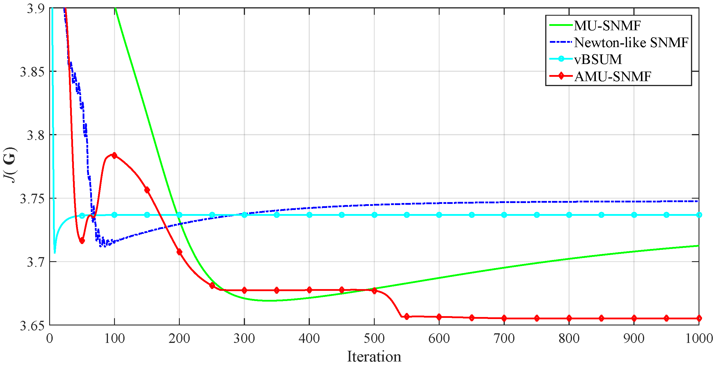
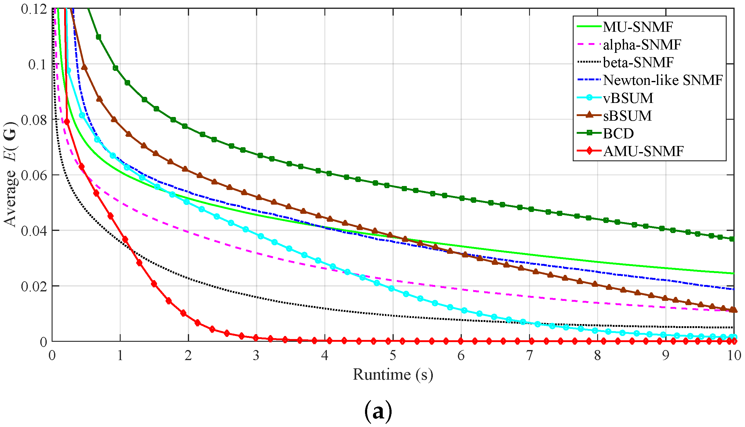
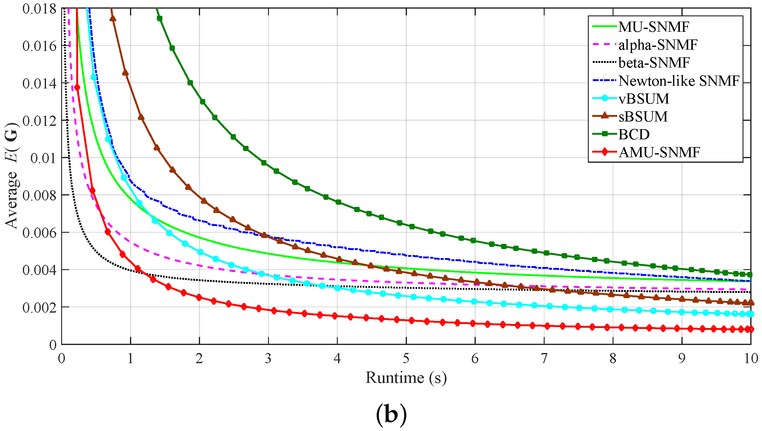
In this section, we first test AMU-SNMF (Algorithm 2) on synthetic data, and then apply it to some real-world clustering problems. Finally, we test AMU-SNMF in SNTF using the framework of the averaging approach [1]. In the clustering experiments, the clustering quality is measured by clustering accuracy (CA) and normalized mutual information (NMI) [19]. CA is used for measuring the percentage of correctly clustered data points. Mutual information (MI) measures the mutual dependence between the predicted and ground truth clustering labels. Furthermore, NMI is a normalization of the MI score to scale the results between 0 (no mutual information) and 1 (perfect correlation). To demonstrate the effectiveness of AMU-SNMF, we compare it with seven SNMF algorithms including MU-SNMF [6], $\alpha$-SNMF [6], $\beta$-SNMF [6], Newton-like SNMF [10] (the code of Newton-like SNMF is available from http://math.ucla.edu/dakuang/), BCD [7], sBSUM [8] and vBSUM [8]. For $\alpha$-SNMF and $\beta$-SNMF algorithms, we use the default setting for the parameters $\alpha$ and $\beta$ recommended by the authors of [6], i.e., $\alpha =0.99$, $\beta =0.99$. In all the experiments, the SNMF algorithms are randomly initialized from points in the form of $\sqrt{\omega }\mathit{P}$ (i.e., ${\mathit{G}}^0=\sqrt{\omega }\mathit{P}$), where $\mathit{P}$ is a randomly generated nonnegative matrix and $\omega ={\mathrm{argmin}}_{\omega \ge 0}\left|\right|A-\omega \mathit{P}{\mathit{P}}^T{\left|\right|}_F^2$. We implement all the experiments on a computer with a 2.8-GHz Intel Core i5-4200 CPU and 8-GB memory by 64-bit MATLAB R2015a on Windows 7.

3.1. Synthetic Data

The synthetic data were generated in the following way: $\mathit{A}=\mathit{G}{\mathit{G}}^T+\mathit{E}$, where $\mathit{G}\in {\mathbb{R}}_{+}^{100\times 30}$ was generated randomly and half of its entries were zeros. $\mathit{E}$ was a matrix of noise whose intensity was determined by signal-to-noise ratio (SNR). We tested AMU-SNMF in both noise-free and noisy scenarios. In the noisy case, the noise level was $\mathrm{SNR}=10$ dB. For each scenario, 20 different $\mathit{A}$ were generated to test AMU-SNMF. To decrease the effect of initializations, the SNMF algorithms were run 10 times with different initializations for each $\mathit{A}$. The SNMF algorithms were stopped when their elapsed time exceeded 10 s. Following the strategy from [20], we report

$$E\left(\mathit{G}\right)=\frac{\left|\right|\mathit{A}-\mathit{G}{\mathit{G}}^T{\left|\right|}_F}{{\left|\right|\mathit{A}\left|\right|}_F}-e_{\min }$$

(11)

of all the SNMF algorithms, where $e_{\min }$ denotes the lowest relative error obtained by any algorithm with any initialization. For the noise-free synthetic data, we use $e_{\min }=0$. The use of $E\left(\mathit{G}\right)$ allows us to take meaningfully the average results over several synthetic data. We compute the average $E\left(\mathit{G}\right)$ over 200 trials (20 different $\mathit{A}$ and 10 different initializations for each $\mathit{A}$), and plot them versus runtime in Figure 2. We can see that in both noise-free and noisy cases (1) it took AMU-SNMF less than 2 s to achieve lower average $E\left(\mathit{G}\right)$ values than that MU-SNMF achieved at the end of the algorithm (10 s), i.e., AMU-SNMF was more than five times faster than MU-SNMF; (2) it took AMU-SNMF less than 4 s to achieve lower average $E\left(\mathit{G}\right)$ values than that the other 6 algorithms (including $\alpha$-SNMF, $\beta$-SNMF, Newton-like SNMF, BCD, sBSUM and vBSUM) achieved at the end of the algorithms (10 s), i.e., AMU-SNMF was more than two times faster than the six algorithms; (3) AMU-SNMF had lower average $E\left(\mathit{G}\right)$ values at the end of the algorithm compared with all the other algorithms. The above observations demonstrate that AMU-SNMF is not only fast but also of high accuracy.

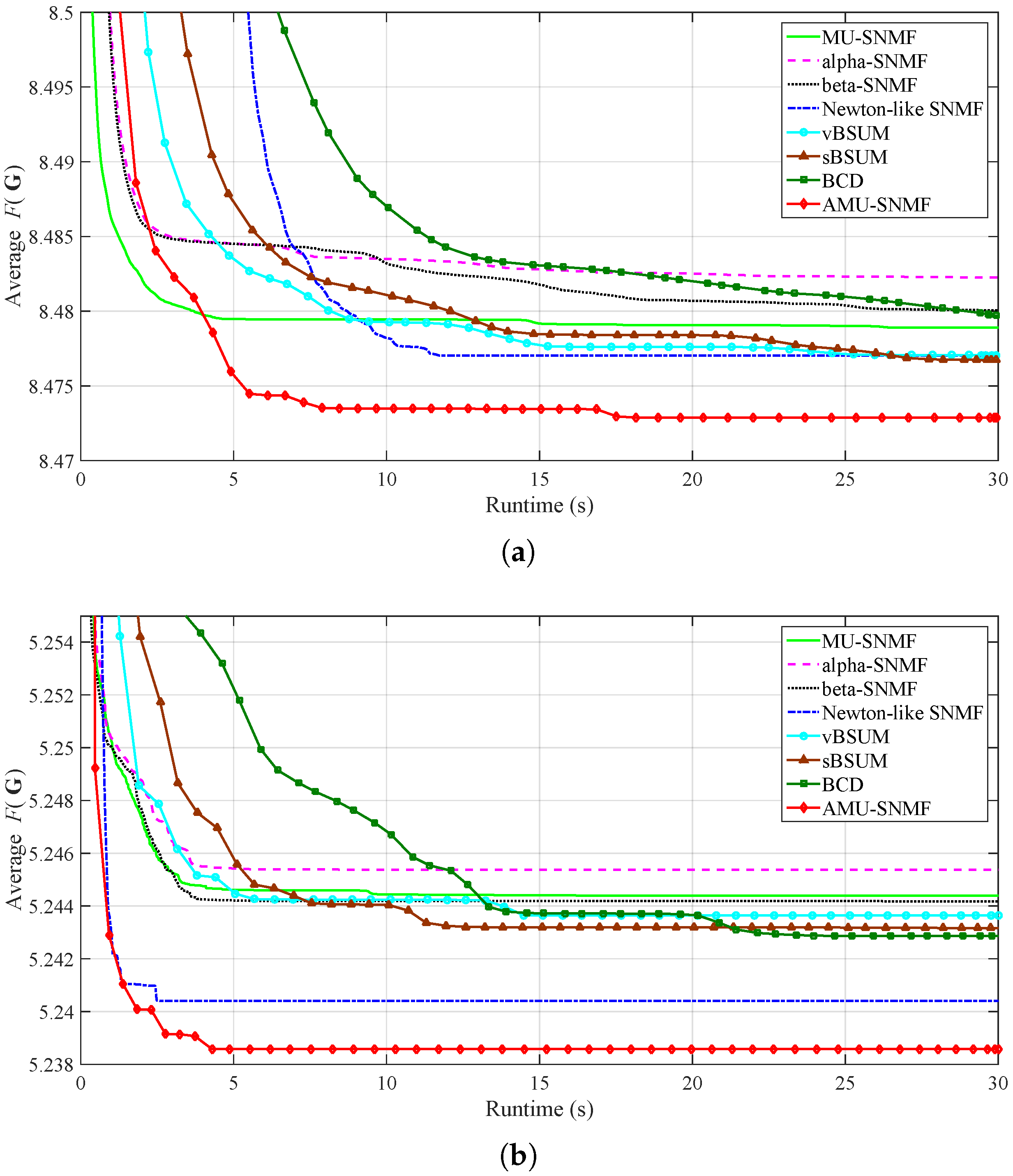
3.2. Document Clustering

In the experiment, we evaluate AMU-SNMF in the applications of document clustering. The goal of document clustering is to organize the documents into different semantic categories automatically [21]. Two widely used document collections, Topic Detection and Tracking 2 (TDT2) (http://projects.ldc.upenn.edu/TDT2/) and Reuters-21578 (http://www.daviddlewis.com/resources/testcollections/reuters21578/), were used here. The TDT2 corpus consists of data collected during the first half of 1998 and taken from six sources: ABC, CNN, VOA, NYT, PRI, and APW. It contains 11,201 documents from 96 semantic categories. The Reuters-21578 corpus was collected from the Reuters newswire in 1987. It contains 21,578 documents from 135 semantic categories. Both collections are highly unbalanced with the sizes of categories ranging from one to thousands of documents. To improve the reliability of our evaluations, we removed those documents appearing in two or more categories and selected 10 categories for each collection. We selected the 10th to 19th largest categories for the TDT2 corpus, and the 12th to 21th largest categories for the Reuters-21578 corpus. The sizes of the selected categories are just a little unbalanced (see

Table 1. The semantic categories from the TDT2 and the Reuters-21578 collections.

TDT2	Category	10	11	12	13	14	15	16	17	18	19
	Number of documents	167	160	145	141	140	131	123	123	120	104
Reuters-21578	Category	12	13	14	15	16	17	18	19	20	21
	Number of documents	63	60	53	45	45	44	42	38	38	37

).

We first normalized each document vector to unit length. Then we constructed the affinity matrix $\mathit{A}$ as follows. Denote the normalized document vectors by ${\mathit{x}}_i\in {\mathbb{R}}^d$, $i=1,2,\dots ,n$. The affinity matrix $\mathit{A}$ was computed by

$${\mathit{A}}_{ij}=\left\{\begin{array}{c}\exp \left(-\frac{\left|\right|{\mathit{x}}_i-{\mathit{x}}_j{\left|\right|}^2}{{\sigma }_i{\sigma }_j}\right),\mathrm{if}i\in \mathcal{N}\left(j\right)\mathrm{or}j\in \mathcal{N}\left(i\right)\hfill \\ 0,\mathrm{otherwise}\hfill \end{array}\right.,$$

(12)

where $\mathcal{N}\left(i\right)=\left\{j\right|{\mathit{x}}_j\mathrm{is}\mathrm{one}\mathrm{of}\mathrm{the}{k}_n\mathrm{nearest}\mathrm{neighbors}\mathrm{of}{\mathit{x}}_i,j\ne i\}$, and the local scale parameter ${\sigma }_i$ of each data point was set to be the distance between ${\mathit{x}}_i$ and its k-th neighbor. We used $k_n=\lfloor {\log }_2\left(n\right)\rfloor +1$ and $k=7$ as suggested in [10,22]. After that, we performed SNMF for document clustering, where every document was assigned to a cluster that had the largest entry in the corresponding row of $\mathit{G}$. To decrease the effect of initializations, the SNMF algorithms were run 20 times with different initializations for each document collection. They were stopped when their elapsed time exceeded 30 s. The plots of the average $F\left(\mathit{G}\right)$ versus runtime are displayed in Figure 3. We can see from Figure 3a that it took AMU-SNMF less than 5 s to achieve lower average $F\left(\mathit{G}\right)$ value than that the other algorithms achieved at the end of the algorithms (30 s). Furthermore, we can see from Figure 3b that (1) all the algorithms converged, and their convergence time was about 15 s (MU-SNMF), 7 s ($\alpha$-SNMF), 5 s ($\beta$-SNMF), 2.5 s (Newton-like SNMF), 25 s (BCD), 15 s (sBSUM), 15 s (vBSUM) and 5 s (AMU-SNMF), respectively; (2) it took AMU-SNMF less than 2 s to achieve lower average $F\left(\mathit{G}\right)$ value than that the other algorithms achieved when they converged. The above observations demonstrate that AMU-SNMF was more than six times faster than MU-SNMF, and more than two times faster than the other algorithms except Newton-like SNMF. The clustering results on TDT2 and Reuters-21578, averaged over 20 trials with different initializations, are shown in

Table 2. The mean of CA and the mean of NMI of the SNMF algorithms on the TDT2 and the Reuters-21578 collections.

		MU-SNMF [6]	$\mathit{\alpha }$-SNMF [6]	$\mathit{\beta }$-SNMF [6]	Newton-Like SNMF [10]	vBSUM [8]	sBSUM [8]	BCD [7]	AMU-SNMF
TDT2	CA	0.9266	0.9035	0.9187	0.9348	0.9299	0.9312	0.9133	0.9631
	NMI	0.9363	0.9197	0.9292	0.9477	0.9450	0.9464	0.9354	0.9625
Reuters-21578	CA	0.6711	0.6803	0.6786	0.6778	0.6671	0.6630	0.6749	0.6877
	NMI	0.6329	0.6380	0.6383	0.6408	0.6365	0.6345	0.6389	0.6449

. We can see that AMU-SNMF had higher, which demonstrates that AMU-SNMF achieved a better clustering performance compared with the other algorithms.

3.3. Object Clustering

In the experiment, we evaluate AMU-SNMF on Columbia Object Image Library (COIL-20) dataset (http://www.cs.columbia.edu/CAVE/software/softlib/coil-20.php). COIL-20 is a database of gray-scale images of 20 objects. The objects were placed on a motorized turntable against a black background. The turntable was rotated through 360 degrees to vary object pose with respect to a fixed camera. Images of the objects were taken at pose intervals of 5 degrees. This corresponds to 72 images per object. Each image is $128\times 128$ pixels in size.

We first constructed the affinity matrix $\mathit{A}$ by (12). Then we performed SNMF for object clustering, where every image was assigned to a cluster that had the largest entry in the corresponding row of $\mathit{G}$. To decrease the effect of initializations, the SNMF algorithms were run 20 times with different initializations. They were stopped when their elapsed time exceeded 30 s. The plot of the average $F\left(\mathit{G}\right)$ versus runtime is displayed in Figure 4. We can see that (1) it took AMU-SNMF about 3.5 s to achieve the average $F\left(\mathit{G}\right)$ value that MU-SNMF achieved when MU-SNMF converged (about 15 s), i.e., AMU-SNMF was more than four times faster than MU-SNMF; (2) AMU-SNMF was more than three times faster than $\alpha$-SNMF, $\beta$-SNMF, BCD, sBSUM and vBSUM. The clustering results, averaged over 20 trials with different initializations, are shown in

Table 3. The mean of CA and the mean of NMI of the SNMF algorithms on the COIL-20 dataset.

		MU-SNMF [6]	$\mathit{\alpha }$-SNMF [6]	$\mathit{\beta }$-SNMF [6]	Newton-Like SNMF [10]	vBSUM [8]	sBSUM [8]	BCD [7]	AMU-SNMF
COIL-20	CA	0.6641	0.6527	0.6890	0.7247	0.7086	0.6657	0.6362	0.7332
	NMI	0.7826	0.7774	0.8160	0.8492	0.8454	0.8166	0.7882	0.8554

. We can see that AMU-SNMF had higher, which demonstrates that AMU-SNMF achieved a better clustering performance compared with the other algorithms.

3.4. SNTF

In the experiment, we test AMU-SNMF in SNTF using the framework of the averaging approach [1], which has been discussed in Section 2.4. The experiment was performed on synthetic data which were generated in the following way: $\mathcal{A}={\sum }_{i=1}^r{\mathit{g}}_i\circ {\mathit{g}}_i\circ {\mathit{g}}_i+\mathcal{E}$, where $r=3$, ${\mathit{g}}_i\in {\mathbb{R}}_{+}^{10}(i=1,2,3)$ were generated randomly, and $\mathcal{E}\in {\mathbb{R}}^{10\times 10\times 10}$ was a symmetric tensor of noise whose intensity was determined by signal-to-noise ratio (SNR). Both noise-free and noisy (SNR = 10 dB) synthetic data were used here with each including 10 different $\mathcal{A}$. The SNTF was performed by the averaging approach where eight different SNMF algorithms were separately used for (10). The averaging approach was stopped when its elapsed time exceeded 0.5 s. To decrease the effect of initializations, 10 trials were conducted by choosing different initializations for each $\mathcal{A}$. We measure the quality of SNTF by

$$Fit\left(\mathit{G}\right)=1-\frac{\left|\right|\mathcal{A}-{\sum }_{i=1}^r{\mathit{g}}_i\circ {\mathit{g}}_i\circ {\mathit{g}}_i\left|\right|}{\left|\right|\mathcal{A}\left|\right|}.$$

(13)

The greater the value of $Fit\left(\mathit{G}\right)$, the better approximation of the tensor $\mathcal{A}$ is obtained by ${\sum }_{i=1}^r{\mathit{g}}_i\circ {\mathit{g}}_i\circ {\mathit{g}}_i$. We compute the average $Fit\left(\mathit{G}\right)$ of the averaging approach over 100 trials (10 different $\mathcal{A}$ and 10 different initializations for each $\mathcal{A}$). The results are listed in

Table 4. The mean of $Fit\left(\mathit{G}\right)$ of the averaging approach using different SNMF algorithms.

	MU-SNMF [6]	$\mathit{\alpha }$-SNMF [6]	$\mathit{\beta }$-SNMF [6]	Newton-Like SNMF [10]	vBSUM [8]	sBSUM [8]	BCD [7]	AMU-SNMF
free noise	0.9464	0.9471	0.9471	0.9430	0.9472	0.9460	0.9460	0.9483
SNR = 10 dB	0.7230	0.7234	0.7234	0.7228	0.7234	0.7230	0.7230	0.7243

. We can see that the averaging approach with AMU-SNMF yielded better approximate tensor than that with other SNMF algorithms in both noise-free and noisy cases.

4. Conclusions

In this paper, we propose an accelerated variant of the MU-SNMF algorithm designed to solve the SNMF problem. The accelerated algorithm is referred to as AMU-SNMF. It is derived by exploiting the extrapolation scheme in NAG and a restart strategy. Our contributions consist of two parts. First, we derive an accelerated variant of the MU-SNMF algorithm. It is numerically shown that AMU-SNMF is more than four times faster than MU-SNMF. Second, we empirically demonstrate that AMU-SNMF outperforms other 6 state-of-the-art algorithms, including $\alpha$-SNMF [6], $\beta$-SNMF [6], Newton-like SNMF [10], BCD [7], sBSUM [8] and vBSUM [8]. The experiment results show that AMU-SNMF is more than two times faster than the above algorithms except the Newton-like SNMF algorithm. Moreover, the experiment results show that AMU-SNMF can achieve a better clustering performance in the real-world clustering problems compared with the above algorithms. Furthermore, AMU-SNMF is more suitable for the averaging approach in SNTF. As one of directions of future work, we plan to investigate further the convergence properties of the AMU-SNMF algorithm. Another direction of future work is that we could apply the methodologies adopted in this paper to other SNMF algorithm.

References

1. Cichocki, A.; Jankovic, M.; Zdunek, R.; Amari, S.I. Sparse super symmetric tensor factorization. In Proceedings of the 2007 International Conference on Neural Information Processing (ICONIP), Kitakyushu, Japan, 13–16 November 2007; pp. 781–790. [Google Scholar]
2. Lu, S.; Hong, M.; Wang, Z. A nonconvex splitting method for symmetric nonnegative matrix factorization: Convergence analysis and optimality. IEEE Trans. Signal Process. 2017, 65, 3120–3135. [Google Scholar] [CrossRef]
3. Gao, T.; Olofsson, S.; Lu, S. Minimum-volume-regularized weighted symmetric nonnegative matrix factorization for clustering. In Proceedings of the 2016 IEEE Global Conference on Signal and Information Processing (GlobalSIP), Washington, DC, USA, 7–9 December 2016; pp. 247–251. [Google Scholar]
4. Marin, M.; Vlase, S.; Paun, M. Considerations on double porosity structure for micropolar bodies. Aip Adv. 2015, 5, 037113. [Google Scholar] [CrossRef] [Green Version]
5. Ma, Y.; Hu, X.; He, T.; Jiang, X. Hessian regularization based symmetric nonnegative matrix factorization for clustering gene expression and microbiome data. Methods 2016, 111, 80–84. [Google Scholar] [CrossRef] [PubMed]
6. He, Z.; Xie, S.; Zdunek, R.; Zhou, G.; Cichocki, A. Symmetric Nonnegative Matrix Factorization: Algorithms and Applications to Probabilistic Clustering. IEEE Trans. Neural Netw. 2011, 22, 2117–2131. [Google Scholar]
7. Vandaele, A.; Gillis, N.; Lei, Q.; Zhong, K.; Dhillon, I. Efficient and Non-Convex Coordinate Descent for Symmetric Nonnegative Matrix Factorization. IEEE Trans. Signal Process. 2016, 64, 5571–5584. [Google Scholar] [CrossRef]
8. Shi, Q.; Sun, H.; Lu, S.; Hong, M.; Razaviyayn, M. Inexact Block Coordinate Descent Methods for Symmetric Nonnegative Matrix Factorization. IEEE Trans. Signal Process. 2017, 65, 5995–6008. [Google Scholar] [CrossRef] [Green Version]
9. Zass, R.; Shashua, A. A unifying approach to hard and probabilistic clustering. In Proceedings of the 2005 International Conference on Computer Vision (ICCV), Beijing, China, 17–20 October 2005; pp. 294–301. [Google Scholar]
10. Kuang, D.; Ding, C.; Park, H. Symmetric Nonnegative Matrix Factorization for Graph Clustering. In Proceedings of the 2012 SIAM International Conference on Data Mining (SDM), Anaheim, CA, USA, 26–28 April 2012; pp. 106–117. [Google Scholar]
11. Kuang, D.; Yun, S.; Park, H. SymNMF: Nonnegative Low-Rank Approximation of a Similarity Matrix for Graph Clustering. J. Glob. Optim. 2015, 62, 545–574. [Google Scholar] [CrossRef]
12. Lu, S.; Wang, Z. Accelerated algorithms for eigen-value decomposition with application to spectral clustering. In Proceedings of the 2015 Asilomar Conference on Signals, Systems and Computers (ACSSC), Pacific Grove, CA, USA, 8–11 November 2015; pp. 355–359. [Google Scholar]
13. Bo, L.; Zhang, Z.; Wu, X.; Yu, P.S. Relational clustering by symmetric convex coding. In Proceedings of the 2007 International Conference on Machine Learning (ICML), Corvallis, OR, USA, 20–24 June 2007; pp. 569–576. [Google Scholar]
14. Long, B.; Zhang, Z.; Yu, P. Co-clustering by block value decomposition. In Proceedings of the 2005 SIGKDD Conference on Knowledge Discovery and Data Mining (SIGKDD), Chicago, IL, USA, 21–24 August 2005; pp. 635–640. [Google Scholar]
15. Nesterov, Y. A method of solving a convex programming problem with convergence rate O(1/k2). Sov. Math. Dokl. 1983, 27, 372–376. [Google Scholar]
16. Sutskever, I.; Martens, J.; Dahl, G.; Hinton, G. On the importance of initialization and momentum in deep learning. In Proceedings of the 2013 International Conference on Machine Learning (ICML), Atlanta Marriott Marquis, Atlanta, GA, USA, 16–21 June 2013; pp. 1139–1147. [Google Scholar]
17. Botev, A.; Lever, G.; Barber, D. Nesterov’s accelerated gradient and momentum as approximations to regularised update descent. In Proceedings of the 2017 International Joint Conference on Neural Networks (IJCNN), Anchorage, AK, USA, 14–19 May 2017; pp. 1899–1903. [Google Scholar]
18. Yudin, D.; Nemirovskii, A.S. Informational complexity and efficient methods for the solution of convex extremal problems. Matekon 1976, 13, 3–25. [Google Scholar]
19. Wu, W.; Jia, Y.; Kwong, S.; Hou, J. Pairwise Constraint Propagation-Induced Symmetric Nonnegative Matrix Factorization. IEEE Trans. Neural Netw. Learn. Syst. 2018, 29, 6348–6361. [Google Scholar] [CrossRef]
20. Ang, A.M.S.; Gillis, N. Accelerating nonnegative matrix factorization algorithms using extrapolation. Neural Comput. 2019, 31, 417–439. [Google Scholar] [CrossRef] [PubMed] [Green Version]
21. Cai, D.; He, X.; Han, J. Document clustering using locality preserving indexing. IEEE Trans. Knowl. Data Eng. 2005, 17, 1624–1637. [Google Scholar] [CrossRef] [Green Version]
22. Zelnik-Manor, L.; Perona, P. Self-Tuning Spectral Clustering. In Proceedings of the Advances in Neural Information Processing Systems, Vancouver, BC, Canada, 13–18 December 2004; pp. 1601–1608. [Google Scholar]
Figure 1. The trajectories of J ( G ) generated by the averaging approach on a three order symmetric nonnegative tensor A R + 10 × 10 × 10 , where 4 different SNMF algorithms were used separately in the averaging approach.
Symmetry 12 01187 g001
Figure 2. The plots of the average E ( G ) versus runtime on the synthetic data. (a) Noise-free. (b) SNR = 10 dB.
Symmetry 12 01187 g002aSymmetry 12 01187 g002b
Figure 3. The plots of the average F ( G ) versus runtime on (a) TDT2 and (b) Reuters-21578.
Symmetry 12 01187 g003
Figure 4. The plot of the average F ( G ) versus runtime on the COIL-20 dataset.
Symmetry 12 01187 g004