Finite Difference Approximation Method for a Space Fractional Convection–Diffusion Equation with Variable Coefficients

Abstract

Space non-integer order convection–diffusion descriptions are generalized form of integer order convection–diffusion problems expressing super diffusive and convective transport processes. In this article, we propose finite difference approximation for space fractional convection–diffusion model having space variable coefficients on the given bounded domain over time and space. It is shown that the Crank–Nicolson difference scheme based on the right shifted Grünwald–Letnikov difference formula is unconditionally stable and it is also of second order consistency both in temporal and spatial terms with extrapolation to the limit approach. Numerical experiments are tested to verify the efficiency of our theoretical analysis and confirm order of convergence.

1. Introduction

Fractional differential equations (FDE) have attracted the attention of many researchers and scientists due to their importance in different fields of study such as viscoelasticity, fluid mechanics, physics, biology, engineering, and flows in porous media (see [1,2,3,4,5,6] and the references cited therein). As different experiments and implementations have shown, non-integer space derivatives have been used to develop anomalous diffusion to which a particle spreads at a rate inconsistent with the integer Brownian motion problem in the direction of both time and space. When non-integer order is replaced by the second order derivative in a diffusion equation, it acts to enhance the process which we call super-diffusion [7,8,9,10,11,12]. Laboratory experiments and field-scale tracer dispersion breakthrough curves (BTCs) are suitable for exhibiting early time arrivals that are not captured by the integer order derivatives and these non-Fickian phenomena can be controlled by non-classical order convection–diffusion and dispersion equations (FCDE) as it was explained in [13]. To increase the number of applications, there should be significant interest in constructing numerical schemes to solve a well known space fractional convection–diffusion model that has space variable coefficients. In most cases, non-integer order differential problems have no exact solution, so various iterative and numerical approximations [3,9,14] must be pointed out in advance. In general, these kinds of approaches have become important in finding the approximate solutions of fractional differential equations, so extensive numerical methods have been developed for space fractional convection–diffusion equations such as the spectral method [15], finite volume method [16,17], finite difference method [2,9,14,18,19,20,21,22,23,24,25,26], finite element method [27,28,29,30] and collocation method [31,32].

When the discretization of domain over the region (which belongs to the geometry) is not complex, finite difference approximations are easier and faster than other methods (see [16,33] for further details) to get numerical solutions. In [34], the author used an unconditional stable difference method for time−space fractional convection–diffusion problems with space variable coefficients with first order convergence both in time and space. The Crank–Nicolson finite difference method for one-sided space fractional diffusion equations using an extrapolation method to get second order convergence was studied in [23]. In [9], the explicit and implicit finite difference methods are discussed for a one-sided space fractional convection–diffusion equation with first order convergence in both time and space. A first-order implicit finite difference discretization method for a two-sided space fractional diffusion equation (SFDE) is also applied in [10]. Recently, an unconditionally stable second order accurate difference method for a two-sided time−space fractional convection–diffusion equation was constructed in [35] using the weighted and Shifted Grünwald–Letnikov difference approximation. It is not suitable to apply the weighted combined with shifted Grünwald–Letnikov difference approximation for one-sided Riemann–Liouville fractional derivative to have second order accurate in space. To deal with such issues, it is important to develop a numerical scheme that leads to evaluate a one-sided space fractional convection–diffusion problem. Thus, the main focus of our study is to have temporal and spatial second order convergence estimates for one-sided space fractional convection–diffusion equations based on a stable finite difference method and using spatial extrapolation to the limit approach. The scheme has been treated using the Crank–Nicholson method with the novel Shifted Grünwald–Letnikov difference approximation and the algorithm has been examined both theoretically and experimentally.

Let us consider space-fractional convection–diffusion equation with variable coefficients:

$$\frac{\partial u(x,t)}{\partial t}+c\left(x\right)\frac{\partial u(x,t)}{\partial x}=d\left(x\right)\frac{{\partial }^{\alpha }u(x,t)}{\partial x^{\alpha }}+p(x,t),x\in (L,R),t\in (0,T],\alpha \in (1,2];$$

(1)

with the given initial condition:

$$u(x,0)=g\left(x\right),L\le x\le R,$$

and homogeneous Dirichlet boundary conditions:

$$u(L,t)=0,u(R,t)=0,0\le t\le T,$$

where $c\left(x\right),d\left(x\right)$ and $g\left(x\right)$ are continuous functions on $[L,R]$ and $p(x,t)$ is continuous function on $[L,R]\times [0,T]$. Here $u(x,t)$ is the concentration, $d\left(x\right)>0$ is the variable diffusion coefficient, $c\left(x\right)>0$ is the fluid variable velocity which means the system is evolving in space due to a velocity field and $p(x,t)$ is sink term so that the fluid transport is from left to right. For the case of integer order ($\alpha =2$), Equation (1) gives to the classical convection–diffusion equation(CDE). In this study, we have only considered the fractional derivative case which describes a physical meaning in [36] and it involves only a left-sided fractional order derivative. We have assumed that this one-dimensional space fractional convection–diffusion problem has sufficiently smooth and unique enough solutions.

The structure of this paper is arranged as follows. In Section 2, we introduce some preliminary remarks, lemmas and definitions and we show the formulation of the new Crank–Nicolson with right Shifted Grünwald–Letnikov difference scheme in Section 3. In Section 4, we describe the unconditional stability using Gerschgorin Theorem and convergence order analysis of the scheme. In Section 5, numerical tests are implemented to show the relevance of our theoretical study and the conclusions are put in Section 6.

2. Preliminary Remarks

Definition 1.

The Riemann fractional derivative operator $D_{\ast }^{\alpha }$ with order α is written as:

$$\left(D_{\ast }^{\alpha }u\right)\left(x\right)={\displaystyle \frac{1}{\mathsf{\Gamma }(r-\alpha )}}{\displaystyle \frac{d^r}{d{x}^r}}{\int }_L^x{\displaystyle \frac{u\left(t\right)}{{(x-t)}^{\alpha -r+1}}}dt,\alpha >0$$

(2)

where $r-1<\alpha <r,r\in N,t>0$.

Definition 2.

The left hand side and the right hand side fractional order derivatives, respectively, in Equation (1) are the Riemann–Liouville fractional derivatives with order α which are given by:

$$\begin{array}{ccc}\hfill \left(D_{+}^{\alpha }u\right)\left(x\right)& =& \frac{1}{\mathsf{\Gamma }(r-\alpha )}\frac{d^r}{d{x}^r}{\int }_L^x{(x-s)}^{r-\alpha -1}u\left(s\right)ds\hfill \\ \hfill \left(D_{-}^{\alpha }u\right)\left(x\right)& =& \frac{{(-1)}^r}{\mathsf{\Gamma }(r-\alpha )}\frac{d^r}{d{x}^r}{\int }_x^R{(s-x)}^{r-\alpha -1}u\left(s\right)ds\hfill \end{array}$$

(3)

for $r-1<\alpha <r,x\in \Re$.

Definition 3

([3]). Let u be given on ℜ. The standard Grünwald–Letnikov estimate for $1<\alpha \le 2$ with positive order α is defined by the formula,

$$D^{\alpha }u(x,t)\approx \frac{1}{h^{\alpha }}\sum _{k=0}^{N_x}{\omega }_k^{\left(\alpha \right)}u(x-kh,t),$$

(4)

we also define the Grünwald–Letnikov difference operator as:

$$h^{-\alpha }\left({\mathsf{\Delta }}_h^{\alpha }u\right)(x,t)\approx \sum _{k=0}^{N_x}{\omega }_k^{\left(\alpha \right)}u(x-kh,t),h>0,x\in \Re ,$$

(5)

where

$${\omega }_k^{\left(\alpha \right)}=\frac{\alpha (\alpha -1)\dots (\alpha -k+1)}{k!},$$

(6)

is called Grünwald–Letnikov coefficient which is the Taylor series expansion $\omega \left(z\right)={(1-z)}^{\alpha }$ which is the generating function. We can expressed the coefficients by the following recursive relations.

$${\omega }_0^{\left(\alpha \right)}=1,{\omega }_k^{\left(\alpha \right)}=(1-\frac{\alpha +1}{k}){\omega }_{k-1}^{\left(\alpha \right)},k=1,2,\dots .$$

(7)

Lemma 1

([37]). Assume that $1<\alpha \le 2$, then Grünwald–Letnikov coefficients ${\omega }_k^{\left(\alpha \right)}$ satisfy:

$$\left\{\begin{array}{c}{\omega }_0^{\left(\alpha \right)}=1,{\omega }_1^{\left(\alpha \right)}=-\alpha <0,{\omega }_2^{\left(\alpha \right)}={\displaystyle \frac{\alpha (\alpha -1)}{2}}>0\hfill \\ 1\ge {\omega }_2^{\left(\alpha \right)}\ge {\omega }_3^{\left(\alpha \right)}\ge \dots \ge 0,\hfill \\ \sum _{k=0}^{\infty }{\omega }_k^{\left(\alpha \right)}=0,\sum _{k=0}^{N_x}{\omega }_k^{\left(\alpha \right)}<0,N_x\ge 1.\hfill \end{array}\right.$$

(8)

The Shifted Grünwald–Letnikov difference operator expression is suitable for our purpose because, it allows us to estimate $\left(D_{\ast }^{\alpha }u\right)\left(x\right)$, which is defined in Equation (2), numerically in an accurate way. According to [14], right shifted Grünwald–Letnikov difference operator with p shifts for ${\alpha }^{th}$ order Left R-L fractional derivative of $u(x,t),x\in [L,R]$ at $x=x_m$ can be expressed as:

$$\begin{array}{ccc}\hfill \left(D_{\ast }^{\alpha }u\right)(x,t)& \approx & \frac{1}{h^{\alpha }}\sum _{k=0}^{\frac{x_m-L}{h}+p}{\omega }_k^{\left(\alpha \right)}u(x-(k-p)h,t)\hfill \end{array}$$

(9)

where

$$\begin{array}{c}\hfill x_m=L+mh,h=\frac{R-L}{N_x},m=0,1,2,\dots N_x.\end{array}$$

Lemma 2

([38,39]). Let $u\in C^{2n}(\Re )$ that has a finite degree of smoothness with $\left(D_{+}^{\alpha }u\right)\left(x\right)$ which is approximated by $h^{-\alpha }\left({\mathsf{\Delta }}_h^{\alpha }u\right)\left(x\right)$ possesses an asymptotic expansion in integer powers of the step-length h, then an expansion in even powers of h for the Shifted operator can be written in the form:

$$\left({\mathsf{\Delta }}_{h,p}^{\alpha }u\right)\left(x\right)=\sum _{j=0}^{\infty }{\left(-1\right)}^j\left({}_j^{\alpha }\right)u\left(x+\frac{\alpha h}{2}-jh\right),h>0.$$

(10)

Lemma 3

([39]). Let $u\in C^{n+3}(\Re )$ all derivative of u up to the order $n+4$ belong to $L^1(\Re )$. Then the Fourier transform of the Grünwald–Letnikov difference operator defined in Equation (5), is

$$\widehat{\varphi }\left(x\right)={\int }_{\Re }\varphi \left(t\right)e^{ixt}dt.$$

(11)

Theorem 1.

Let $u\in C^{2n+3}(\Re )$ with all derivatives of u up to order $2n+3$ belong to $L^1(\Re )$. For $p\ge 0$ define the shifted Grünwald–Letnikov operator:

$$\left({\mathsf{\Delta }}_{h,p}^{\alpha }\right)u\left(x\right)=\sum _{k=0}^{\infty }{\omega }_k^{\left(\alpha \right)}u\left(x-\left(k-p\right)h\right),$$

with ${\omega }_k^{\left(\alpha \right)}$=${(-1)}^{2k}$$\left(\genfrac{}{}{0pt}{}{\alpha }{a_{2k}}\right)$=$\left(\genfrac{}{}{0pt}{}{\alpha }{a_{2k}}\right)$. Then, if $L=-\infty$ in Equation (2), for any computable coefficient $a_{2k}$, which is independent of $h,u$ and x, we have

$$h^{-\alpha }\left({\mathsf{\Delta }}_{h,p}^{\alpha }u\right)\left(x\right)=\left(D_{+}^{\alpha }u\right)\left(x\right)+\sum _{k=1}^{n-1}{b}_{2k}\left(D_{+}^{\alpha +2k}u\right)\left(x\right)h^{2k}+O\left(h^{2n}\right)$$

uniformly in $x\in \Re$.

Proof of Theorem 1.

We closely follow the result described in [9,10] for the unshifted Grünwald–Letnikov formula and also in [23] for the shifted Grünwald–Letnikov formula. We can see that with the Riemann-Lebesgue lemma, the assumptions on u indicates for real positive constant $C_1$ and from the condition which is imposed on u, we have

$$\left|\tilde{u}\left(t\right)\right|\le C_1{(1+|t\left|\right)}^{-2n-3}.$$

(12)

From Lemma 3 for all $t\in \Re$ the Fourier transform for $u\left(x\right)$ of the Grünwald–Letnikov approximation is

$$\tilde{u}\left(t\right)={\int }_{\Re }u\left(x\right)e^{ixt}dx.$$

From the definition of Fourier transform, we have observed that for a constant $a\in \Re$, we have:

$$\mathcal{F}\left(\left[u(x-a)\right]\right)\left(t\right)=e^{iat}\tilde{u}\left(t\right).$$

The function

$${\left(\frac{1-e^{-z}}{z}\right)}^{\alpha }{e}^{zp}={\omega }_{\alpha ,p}\left(z\right),$$

have the Taylor expansion

$${\omega }_{\alpha ,p}\left(z\right)=\sum _{k=0}^{\infty }{a}_{2k}{z}^{2k},$$

(13)

where $a_{2k}$=${(-1)}^{2k}$$\left(\genfrac{}{}{0pt}{}{\alpha }{a_{2k}}\right)$=$\left(\genfrac{}{}{0pt}{}{\alpha }{a_{2k}}\right)$, converges absolutely for $\left|z\right|\le 1$ since the function ${\omega }_{\alpha ,p}\left(z\right)$ is bounded on ℜ. The shifted Grünwald difference approximation $\left({\mathsf{\Delta }}_{h,p}\right)u\left(x\right)\in L^1(\Re )$.

Thus, we have

$$\begin{array}{ccc}\hfill \mathcal{F}\left(h^{-\alpha }{\mathsf{\Delta }}_{h,p}^{\alpha }u\right)\left(t\right)& =& h^{-\alpha }{e}^{-itph}\sum _{k=0}^{\infty }\left({}_{2k}^{\alpha }\right)e^{ikth}\tilde{u}\left(t\right)\hfill \\ \hfill & =& h^{-\alpha }{e}^{-itph}{\left(1-e^{itph}\right)}^{\alpha }\tilde{u}\left(t\right)\hfill \\ \hfill & =& {(-it)}^{\alpha }{\left(\frac{1-e^{ith}}{-ith}\right)}^{\alpha }{e}^{-itph}\tilde{u}\left(t\right)={(-it)}^{\alpha }{\omega }_{\alpha ,p}(-ith)\tilde{u}\left(t\right)\hfill \end{array}$$

(14)

since ${\omega }_{\alpha ,p}(-ith)$ is analytic around the origin, we express it as an even power expansions

$${\omega }_{\alpha ,p}\left(z\right)=\sum _{k=0}^{\infty }{a}_{2k}{z}^{2k}$$

which absolutely convergent for all $\left|z\right|\le R$. For this a bounded function ${\omega }_{\alpha ,p}\left(z\right)$ on ℜ, there exist a real positive constant $C_2$ which satisfy:

$$\left|{\left(\frac{1-e^{ix}}{-ix}\right)}^{\alpha }-\sum _{k=0}^{n-1}{a}_{2k}{\left(-ix\right)}^{2k}\right|\le C_2{\left|x\right|}^{2n}$$

(15)

is bounded uniformly in $x\in \Re$. For any value $\left|x\right|\le R$, we have

$$\begin{array}{c}\hfill \left|({\omega }_{\alpha ,p}(-ix)-\sum _{k=0}^{n-1}{a}_{2k}{(-ix)}^{2k}\right|=\left|\sum _{k=n}^{\infty }{a}_{2k}{(-ix)}^{2k}\right|\le {\left|x\right|}^{2n}\sum _{k=n}^{\infty }\left({}_{a_{2k}}^{\alpha }\right){\left|x\right|}^{2(k-n)}\le C_3{\left|x\right|}^{2n}\end{array}$$

(16)

which is bounded on ℜ. For the other case $\left|x\right|>R$ also, we have

$$\left|{\omega }_{\alpha ,p}\left(-ix\right)\right|=\left|{\left(\frac{1-e^{ix}}{-ix}\right)}^{\alpha }{e}^{ipx}\right|\le \frac{2^{\alpha }}{R^{\alpha }}<C_4{\left|x\right|}^{2n}$$

(17)

where $C_4=\frac{2^{\alpha }}{R^{\alpha +2n}}<\infty$ and also

$$\left|\sum _{k=0}^{n-1}{a}_{2k}{(-ix)}^{2k}\right|\le {\left|x\right|}^{2n}\sum _{k=0}^{n-1}|({}_{a_{2k}}^{\alpha })|{\left|x\right|}^{2(k-n)}\le C_5{\left|x\right|}^{2n}$$

(18)

with $C_5={\sum }_{k=0}^{n-1}\left|\left({}_{a_{2k}}^{\alpha }\right)\right|R^{2k-2n}<\infty$. Now, we set that

$$C_2=max\left\{\sum _{k=0}^{\infty }\left|a_{2k}\left|R^{2k-2n},\frac{2^{\alpha }}{R^{\alpha +2n}}+\sum _{k=0}^{n-1}\right|a_{2k}\right|R^{2k-2n}\right\}$$

since

$$\sum _{k=0}^{\infty }\left|a_{2k}\right|R^{2k-2n}=\sum _{k=0}^{n-1}\left|a_{2k}\right|R^{2k-2n}+\sum _{k=n}^{\infty }\left|a_{2k}\right|R^{2k-2n}$$

$$C_2=\frac{2^{\alpha }}{R^{\alpha +2n}}+\sum _{k=0}^{n-1}\left|a_{2k}\right|R^{2k-2n}$$

Then, this implies that Equation (15) holds for all $x\in \Re$. From Equation (17), we can write

$$\mathcal{F}\left(h^{-\alpha }{\mathsf{\Delta }}_{h,p}^{\alpha }u\right)\left(t\right)=\sum _{k=0}^{n-1}{a}_{2k}{\left(-it\right)}^{\alpha +2k}{h}^{2k}\tilde{u}\left(t\right)+\tilde{\phi }(t,h)$$

where

$$\tilde{\phi }(k,h)={\left(-it\right)}^{\alpha }\left({\omega }_{\alpha ,p}\left(-ith\right)-\sum _{k=0}^{n-1}{a}_{2k}{\left(-ith\right)}^{2k}\right)\tilde{u}\left(t\right)$$

since

$${\left(-it\right)}^{\alpha +2k}\tilde{u}\left(t\right)=\left(D_{+}^{\alpha +2k}\right)\tilde{u}\left(t\right).$$

Therefore, we have

$${(-it)}^{\alpha +2k}\tilde{u}\left(t\right)\in L^1(\Re ).$$

Moreover, we see that

$$\tilde{\phi }(t,h)\in L^1(\Re ),$$

and with the conditions imposed on u, we can say that $(1+{\left|x\right|}^{2n+3}\tilde{u}\left(t\right)$ is bounded on ℜ.

Thus, ${\left|t\right|}^{2\alpha -3}\left|\tilde{u}\left(t\right)\right|\in L^1\left(R\right)$. This implies that,

$$\left|\tilde{\phi }(t,h)\right|\le C{h}^{2n}{\left(1+\left|t\right|\right)}^{2\alpha -3}$$

for $k\in \Re$ with $C=C_1{C}_2$. Therefore using the Fourier inversion transform, we have

$$h^{-\alpha }\left({\mathsf{\Delta }}_{h,p}^{\alpha }u\right)\left(x\right)=\left(D_{+}^{\alpha }u\right)\left(x\right)+\sum _{k=1}^{n-1}{a}_{2k}\left(D_{+}^{\alpha +2k}u\right)\left(x\right)h^{2k}+\phi (x,h),$$

where

$$\phi (x,h)=\left|C{\int }_R{e}^{-itx}\tilde{\phi }(t,h)dt\right|\le C{\int }_R\left|\tilde{\phi }(t,h)dt\right|\le C{h}^{2n}.$$

At last, we have

$$h^{-\alpha }\left({\mathsf{\Delta }}_{h,p}^{\alpha }u\right)\left(x\right)=\left(D_{+}^{\alpha }u\right)\left(x\right)+\sum _{k=1}^{n-1}{a}_{2k}\left(D_{+}^{\alpha +2k}u\right)\left(x\right)h^{2k}+O\left(h^{2n}\right).$$

(19)

 □

Remark 1.

From Equation (10), it can be seen that for $p=\alpha /2$, the error takes its minimum value and a second order convergence is achieved. We need the grid points $x_m-(k-p)h$ to find an optimal positive integer p that makes $p-\alpha /2$ is minimum. It is numerically proved in [3] that for the value $0<\alpha \le 1,p=0$ is acceptable; while for $1<\alpha \le 2,p=1$ is optimal.

Remark 2.

Theorem 1 is the base of Extrapolation to the limit. Therefore one can apply it the Shifted Grünwald–Letnikov difference operator to obtain the convergence rate with arbitrary high order $h^k,k=1,2,3,\dots ,n$ such that

$$h^{-\alpha }\frac{\left(q^{-\alpha }{\mathsf{\Delta }}_{qh,p}^{\alpha }u\right)\left(x\right)-q\left({\mathsf{\Delta }}_{h,p}^{\alpha }u\right)\left(x\right)}{1-q},0<q<1$$

(q is fixed) converges to $\left(D_{+}^{\alpha }u\right)\left(x\right)+O(h^2$).

3. Problem Formulation of the Scheme

Consider the following one-dimensional space fractional convection–diffusion problem:

$$\left\{\begin{array}{cc}{\displaystyle \frac{\partial u(x,t)}{\partial t}}=-c\left(x\right){\displaystyle \frac{\partial u(x,t)}{\partial x}}+d\left(x\right){\displaystyle \frac{{\partial }^{\alpha }u(x,t)}{\partial x^{\alpha }}}+p(x,t),\hfill & (x,t)\in (L,R)\times (0,T]\hfill \\ u(x,0)=g\left(x\right),\hfill & x\in [L,R]\hfill \\ u(L,t)=0,u(R,t)=0,\hfill & t\in [0,T]\hfill \end{array}\right.$$

(20)

which is based on shifted Grünwald–Letnikov difference method with $1<\alpha \le 2$ on a finite domain $L<x<R$.

Crank–Nicolson Scheme for Time and Shifted Grünwald Difference Scheme for Space Discretization

We partition the finite interval $[L,R]$ with a uniform mesh in the space size step $h=(R-L)/N_x$ and the time step $\tau =T/N_t$, in which $N_x,N_t$ are non-negative integers and the set of grid size points is symbolized by $x_m=mh$ and $t_n=n\tau$ for $0\le m\le N_x$, $0\le n\le N_t$. Set $t_{n+1/2}=(t_{n+1}+t_n)/2$ with $0\le n\le N_t-1$.

We use the following notations:

$u_m^n=u(x_m,t_n),p_m^{n+1/2}=p(x_m,t_{n+1/2}),{\delta }_t{u}_m^n={\displaystyle \frac{u_m^{n+1}-u_m^n}{\tau }},c_m=c\left(x_m\right),d_m=d\left(x_m\right).$

Applying the C-N technique for the time discretization of Equation (20) gives to

$$\begin{array}{ccc}\hfill {\delta }_t{u}_m^n& =& -{\displaystyle \frac{c_m}{4h}}\left(u_{m+1}^{n+1}-u_{m-1}^{n+1}+u_{m+1}^n-u_{m-1}^n\right)\hfill \\ & +& {\displaystyle \frac{d_m}{2h^{\alpha }}}\sum _{z=0}^1\sum _{k=0}^{N_x-1}{\omega }_k^{\left(\alpha \right)}\left(u_{m-k+1}^{n+z}\right)=p_m^{n+1/2}+O\left({\tau }^2\right).\hfill \end{array}$$

(21)

In space discretization we have used the central finite difference method for the convection term and the Shifted Grünwald–Letnikov operator for the space fractional derivative with the approach of spatial Extrapolation to the limit, respectively.

See the full discretization of the scheme:

$$\begin{array}{ccc}\hfill \frac{u_m^{n+1}-u_m^n}{\tau }& =& \frac{-c_m\left(u_{m+1}^n-u_{m-1}^n+u_{m+1}^{n+1}-u_{m-1}^{n+1}\right)}{4h}\hfill \\ & & +\frac{d_m}{2h^{\alpha }}\left(\sum _{z=0}^1\sum _{k=0}^{m+1}{\omega }_k^{\left(\alpha \right)}{u}_{m-k+1}^{n+z}\right)+\frac{p_m^n+p_m^{n+1}}{2}.\hfill \end{array}$$

(22)

Multiplying Equation (22) by $\tau$ the discretization equation, we have

$$\begin{array}{ccc}\hfill u_m^{n+1}-u_m^n& =& \frac{-c_m\tau }{4h}(u_{m+1}^n-u_{m-1}^n+u_{m+1}^{n+1}-u_{m-1}^{n+1})+\hfill \\ & & \frac{d_m\tau }{2h^{\alpha }}\sum _{z=0}^1\sum _{k=0}^{m+1}{\omega }_k^{\left(\alpha \right)}{u}_{m-k+1}^{n+z}+\tau p_m^{n+1/2}\hfill \end{array}$$

(23)

The above equation is used to predict the values of $u(x,t)$ at time $n+1$, so all the values of u at time n are assumed to be known. For simplification

${\mu }_m=\frac{c_m\tau }{h},{\eta }_m=\frac{d_m\tau }{h^{\alpha }}$, then we have

$$\begin{array}{cc}\hfill & \left(1-\frac{{\eta }_m}{2}{\omega }_1^{\alpha }\right)u_m^{n+1}+\left(\frac{-{\mu }_m}{2}-\frac{{\eta }_m}{2}{\omega }_2^{\alpha }\right)u_{m-1}^{n+1}\hfill \\ & +\left(-\frac{{\mu }_m}{2}-\frac{{\eta }_m}{2}{\omega }_0^{\alpha }\right)u_{m+1}^{n+1}-\frac{{\eta }_m}{2}\left(\sum _{k=3}^{m+1}{\omega }_k^{\alpha }{u}_{m-k+1}^{n+1}\right)\hfill \\ =& \left(1+\frac{{\eta }_m}{2}{\omega }_1^{\alpha }\right)u_m^n+\left(\frac{{\mu }_m}{2}+\frac{{\eta }_m}{2}{\omega }_2^{\alpha }\right)u_{m-1}^n\hfill \\ & +\left(\frac{{\eta }_m}{2}{\omega }_0^{\alpha }+\frac{{\mu }_m}{2}\right)u_{m+1}^n+\frac{{\eta }_m}{2}\left(\sum _{k=3}^{m+1}{\omega }_k^{\left(\alpha \right)}{u}_{m-k+1}^n\right)+\tau \left(p_m^{n+\frac{1}{2}}\right).\hfill \end{array}$$

(24)

Both the convection and diffusion variable coefficients are $(N_x-1)\times (N_x-1)$ diagonal matrices which are defined by

$$\begin{array}{ccc}\hfill {\mu }_m& =& \frac{\tau }{2h}diag\left(C_1,C_2,C_3,\dots C_{N_x-1}\right),\hfill \\ \hfill {\eta }_m& =& \frac{\tau }{h^{\alpha }}diag\left(d_1,d_2,d_3,\dots d_{N_x-1}\right).\hfill \end{array}$$

These discretization together with Dirichlet boundary conditions which results in a linear system of equations for which the coefficient matrix is the sum of lower triangular and upper-diagonal matrices. The above discretization can be re-arranged to yield:

$$\begin{array}{cc}& \left(1-\frac{{\eta }_m}{2}{\omega }_1^{\alpha }\right)u_m^{n+1}+(-\frac{{\mu }_m}{2}-\frac{{\eta }_m}{2}{\omega }_2^{\alpha })u_{m-1}^{n+1}+\hfill \\ & \left(-\frac{{\mu }_m}{2}-\frac{{\eta }_m}{2}{\omega }_0^{\alpha })u_{m+1}^{n+1}-\frac{{\eta }_m}{2}(\sum _{k=3}^{m+1}{\omega }_k^{\alpha }{u}_{m-k+1}^{n+1}\right)\hfill \\ =& (1+\frac{{\eta }_m}{2}{\omega }_1^{\alpha })u_m^n+\left(\frac{{\mu }_m}{2}+\frac{{\eta }_m}{2}{\omega }_2^{\alpha }\right)u_{m-1}^n\hfill \\ & +(\frac{{\eta }_m}{2}{\omega }_0^{\alpha }+\frac{{\mu }_m}{2})u_{m+1}^n+\frac{{\eta }_m}{2}\left(\sum _{k=3}^{m+1}{\omega }_k^{\alpha }{u}_{m-k+1}^n\right)+\tau \left(P_m^{n+\frac{1}{2}}\right).\hfill \end{array}$$

(25)

Denoting $U_m^n$ as the numerical approximation of $u_m^n$, we can construct the C-N scheme for Equation (20)

$$\begin{array}{cc}\hfill & \left(1-\frac{{\eta }_m}{2}{\omega }_1^{\alpha }\right)U_m^{n+1}+\left(-\frac{{\mu }_m}{2}-\frac{{\eta }_m}{2}{\omega }_2^{\alpha }\right)U_{m-1}^{n+1}+\hfill \\ & \left(-\frac{{\mu }_m}{2}-\frac{{\eta }_m}{2}{\omega }_0^{\alpha }\right)U_{m+1}^{n+1}-\frac{{\eta }_m}{2}\left(\sum _{k=3}^{m+1}{\omega }_k^{\alpha }{U}_{m-k+1}^{n+1}\right)\hfill \\ =& \left(1+\frac{{\eta }_m}{2}{\omega }_1^{\alpha }\right)U_m^n+\left(\frac{{\mu }_m}{2}+\frac{{\eta }_m}{2}{\omega }_2^{\alpha }\right)U_{m-1}^n\hfill \\ & +\left(\frac{{\eta }_m}{2}{\omega }_0^{\alpha }+\frac{{\mu }_m}{2}\right)U_{m+1}^n+\frac{{\eta }_m}{2}\left(\sum _{k=3}^{m+1}{\omega }_k^{\alpha }{U}_{m-k+1}^n\right)+\tau \left(P_m^{n+\frac{1}{2}}\right).\hfill \end{array}$$

(26)

I is the $\left(N_x-1\right)\times \left(N_t-1\right)$ identity matrix with $A_{m,n}$ as the matrix coefficients. These coefficients, for $m=1,2,3,\dots ,N_x-1,n=1,2,\dots ,N_t-1$ are given by:

$$A_m{,}_n=\left\{\begin{array}{cc}0,\hfill & n\ge m+2\hfill \\ -\frac{{\mu }_m}{2}-\frac{{\eta }_m}{2}{\omega }_0^{\left(\alpha \right)},\hfill & n=m+1\hfill \\ (1-\frac{{\eta }_m}{2}{\omega }_1^{\left(\alpha \right)}),\hfill & n=m\hfill \\ (-\frac{{\eta }_m}{2}{\omega }_2^{\left(\alpha \right)}-\frac{{\mu }_m}{2}),\hfill & n=m-1\hfill \\ -\frac{{\eta }_m}{2}{\omega }_{m-n+1}^{\left(\alpha \right)}\hfill & n\le m-1.\hfill \end{array}\right.$$

(27)

The finite difference scheme (24) and (26) defines a linear system of equations as

$$\begin{array}{ccc}\hfill (I+A)U^{n+1}& =& (I-A)U^n+\tau \left(p_m^{n+\frac{1}{2}}\right)\hfill \\ \hfill U^{n+1}& =& {[u_1^{n+1},u_2^{n+1},\dots ,u_{N_x-1}^{n+1}]}^{\top }\hfill \\ \hfill U^n+\tau P_m^{n+\frac{1}{2}}& =& {[0,\tau p_1^{n+\frac{1}{2}},\tau p_2^{n+\frac{1}{2}},\dots ,\tau p_{N_x-1}^{n+\frac{1}{2}}+(\frac{{\eta }_{N_x-1}}{2}+\frac{{\mu }_{N_x-1}}{2}),0]}^{\top }.\hfill \end{array}$$

(28)

Theorem 2.

Suppose that $1<\alpha \le 2$, the coefficient matrix defined in Equations (24)–(27), then the diagonal matrix and the coefficient matrix satisfy:

$$A_{m,m}>\sum _{n=0,m\ne 1}^{N_x-1}\left|A_{m,n}\right|,m=1,2,3,\dots ,N_x-1.$$

(29)

Proof of Theorem 2.

As we have seen from the coefficient matrix defined in Equation (27),

$A_{m,m+1}={\displaystyle \frac{{\mu }_m}{2}}-{\displaystyle \frac{{\eta }_m}{2}}{\omega }_0^{\left(\alpha \right)}={\displaystyle \frac{{\mu }_m}{2}}-{\displaystyle \frac{{\eta }_m}{2}}<0$

$A_{m,m-1}=-{\displaystyle \frac{{\eta }_m}{2}}{\omega }_2^{\left(\alpha \right)}-{\displaystyle \frac{{\mu }_m}{2}}=-{\displaystyle \frac{{\eta }_m}{2}}\left({\displaystyle \frac{{\alpha }^2-\alpha }{2}}\right)$, but from Lemma 1, ${\displaystyle \frac{{\alpha }^2-\alpha }{2}}>0$ for $1<\alpha \le 2$ mean that $-{\displaystyle \frac{{\eta }_m}{2}}\left({\displaystyle \frac{{\alpha }^2-\alpha }{2}}\right)<0$.

When $n<m-1$, we have, $-\frac{{\eta }_m}{2}{\omega }_{m-n+1}^{\left(\alpha \right)}<0$ and when $n=m,A_{m,m}=1-{\displaystyle \frac{{\eta }_m}{2}}{\omega }_1^{\left(\alpha \right)}=1+{\displaystyle \frac{{\eta }_m}{2}}\alpha >0$. This implies that ${\sum }_{n=0,m\ne 1}^{N_x-1}\left|A_{m,n}\right|<A_{m,m}$.

Therefore, the diagonal matrix is strictly dominant. □

4. Theoretical Analysis of Finite Difference Scheme

In general for analyzing convergence and stability, we consider the following description.

Let ${\chi }_h=\left\{\nu :\nu =\left\{{\nu }_m\right\}:{\left\{x_m=mh\right\}}_{m=0}^{N_x},{\nu }_0={\nu }_{N_x}=0\right\}$ be the grid function.

For any $\nu ={\nu }_m\in {\chi }_h$, we define our point-wise maximum norm as

$${\left|\right|\nu \left|\right|}_{\infty }=ma{x}_{1\le m\le N_x}\left|{\nu }_m\right|,$$

(30)

and the discrete $L^2$-norm

$$∥\nu ∥=\sqrt{h\sum _{m=1}^{N_x-1}}{\nu }_m^2.$$

(31)

4.1. Boundedness of the Fractional Scheme

The Classical Crank–Nicolson scheme combines the stability of an implicit finite difference method with its accuracy which produce second order convergence in both space and time.

Theorem 3.

Crank–Nicolson scheme for solving space fractional convection–diffusion equations given by the following problem:

$$\frac{\partial u(x,t)}{\partial t}+c\left(x\right)\frac{\partial u(x,t)}{\partial x}=d\left(x\right)\frac{{\partial }^{\alpha }u(x,t)}{\partial x^{\alpha }}+p(x,t).$$

(32)

which is based on shifted Grünwald–Letnikov difference approximation scheme is bounded for $1<\alpha \le 2$.

Proof of Theorem 3.

Consider C-N scheme for the space-fractional convection–diffusion problem for $1<\alpha \le 2$

$$\begin{array}{ccc}\hfill \frac{u_m^{n+1}-u_m^n}{\tau }& =& \frac{-c_m\left(u_m^n-u_{m-1}^n+u_m^{n+1}-u_{m-1}^{n+1}\right)}{2h}\hfill \\ & & +\frac{d_m}{2h^{\alpha }}\left(\sum _{j=0}^1\sum _{k=0}^{m+1}{\omega }_k^{\left(\alpha \right)}{u}_{m-k+1}^{n+j}\right)+\frac{p_m^n+p_m^{n+1}}{2}.\hfill \end{array}$$

(33)

Here, we have shown the convergence and boundedness of the scheme by taking the smaller time-step in terms of Lax–Richtmyer stability analysis that uses a weaker bound (see [40]). Our matrix A has an eigenvalues of $\lambda$ that have positive real parts, and, we also have found a strictly dominant matrix. These eigenvalues which are centered in the disks at each diagonal entries as:

$$A_{m,m}=(1-\frac{{\eta }_m}{2}{\omega }_1^{\alpha })=\left(1+\alpha \frac{{\eta }_m}{2}\right).$$

with ${\mu }_m=\frac{c_m\tau }{h},{\eta }_m=\frac{\tau d_m}{h^{\alpha }}$. From the Gerschgorin Theorem in [41], the radius of the matrix can be expressed as

$$\begin{array}{ccc}\hfill {∥\sum _{n=0,m\ne 1}^{N_x}{A}_{m,n}∥}_2^2& =& {∥\left(-\frac{{\eta }_m}{2}-\frac{{\mu }_m}{2}\right)\sum _{n=0}^{m+1}{\omega }_{m-n+1}^{\left(\alpha \right)}∥}^2\hfill \\ & \le & {∥\left(-\frac{{\eta }_m}{2}-\frac{{\mu }_m}{2}\right)∥}^2{∥\sum _{n=0}^{m+1}{\omega }_{m-n+1}^{\left(\alpha \right)}∥}^2.\hfill \end{array}$$

Since from the Grünwald coefficients we have ${\omega }_{m-n+1}^{\left(\alpha \right)}\le {\omega }_1^{\left(\alpha \right)}$ and ${\omega }_1^{\left(\alpha \right)}=-\alpha$, we have that:

$$\begin{array}{ccc}\hfill {∥\sum _{n=0,m\ne 1}^{N_x}\left(A_{m,n}\right)∥}_2^2& \le & {\left|\sum _{n=0,m\ne 1}^{N_x}\left(A_{m,m}\right)\right|}_2^2\le {∥A_{m,m}∥}_2^2\hfill \\ & \le & {∥(-\frac{{\eta }_m}{2}-\frac{{\mu }_m}{2})∥}_2^2{∥{\omega }_1^{\left(\alpha \right)}∥}_2^2\le {∥1+\frac{{\eta }_m}{2}\alpha ∥}_2^2.\hfill \end{array}$$

For a bounded ratio of time-step $\tau$ and space-step h with $n\tau \le T$, we have

$${∥{\left(A_{m,m}\right)}^n∥}_2\le {\left(1+\frac{{\eta }_m}{2}\alpha \right)}^{n/2}.$$

From the relation of Parseval’s Theorem, [40]

$${∥A_{m,m}∥}_2\le {\left(1+\frac{{\eta }_m}{2}\alpha \right)}^{n/2}\le e^{\alpha T/2}.$$

which shows that the scheme is bounded. □

4.2. Stability Analysis

Theorem 4.

Let $U_m^n$ be the numerical approximation of the exact solution $u_m^n$, then the C-N finite difference scheme (28) is unconditionally stable.

Proof of Theorem 4.

Consider the matrix coefficient of the difference approximation for the problem (20) can be written as described above

$$(I+A)U^{n+1}=(I-A)U^n+\tau p_m^{n+1/2}.$$

(34)

Let $e^n=\left\{e_1^n,e_2^n,e_3^n,\dots ,e_{N_x-1}^n\right\}$, and take the relation between the error $e^{n+1}$ in $U^{n+1}$ and the error $e^n$ in $U^n$ which is given by the linear system

$$e^{n+1}={(I+A)}^{-1}(I-A)e^n.$$

(35)

First of all, we must show that the (non-real valued) eigenvalues of the coefficient matrices A have positive real parts. For ${\omega }_1^{\left(\alpha \right)}=-\alpha$ with fractional order $1<\alpha <2$ and $k\ne 1$; we have ${\omega }_k^{\left(\alpha \right)}>0$. In addition to this, $-{\omega }_1^{\alpha }=\alpha \ge {\sum }_{k=0,k\ne 1}^N{\omega }_k^{\alpha }$ for the value $N>1$. As stated in Gerschgorin Theorem ([41], pp. 136–139), the eigenvalues of the given matrix A are inside the disks centered at each diagonal entry.

$$A_{m,m}=(1-\frac{{\eta }_m}{2}{\omega }_1^{\left(\alpha \right)})=1+\frac{{\eta }_m}{2}\alpha >0,$$

with radius

$$r_m=\sum _{n=0,m\ne 1}^{N_x}\left|A_{m,n}\right|=\frac{{\eta }_m}{2}\sum _{n=0}^{m+1}{\omega }_{m-n+1}^{\left(\alpha \right)}<(1+\frac{{\eta }_m}{2}).$$

These Gerschgorin disks are belong to the right half of the complex plane. Thus, the eigenvalue of the coefficient matrix A has positive real part which implies that A has an eigenvalue $\lambda$ if and only if $(I-A)$ has an eigenvalue $(1-\lambda )$ if and only if ${(I+A)}^{-1}(I-A)$ has an eigenvalue $\left(\frac{1-\lambda }{1+\lambda }\right)$. From the first part of this sentence, we have seen that all the eigenvalues of the matrix given by $(I+A)$ have a radius larger than unity which implies the matrix is invertible. Now we can see from the above description the real part of $\lambda$ is non-negative which we can conclude that $\left|\frac{(1-\lambda )}{(1+\lambda )}\right|<1$.

Thus, the spectral radius of the system matrix ${(I+A)}^{-1}(I-A)$ is strictly less than unity which implies that the difference scheme is unconditionally stable. □

4.3. Convergence Analysis

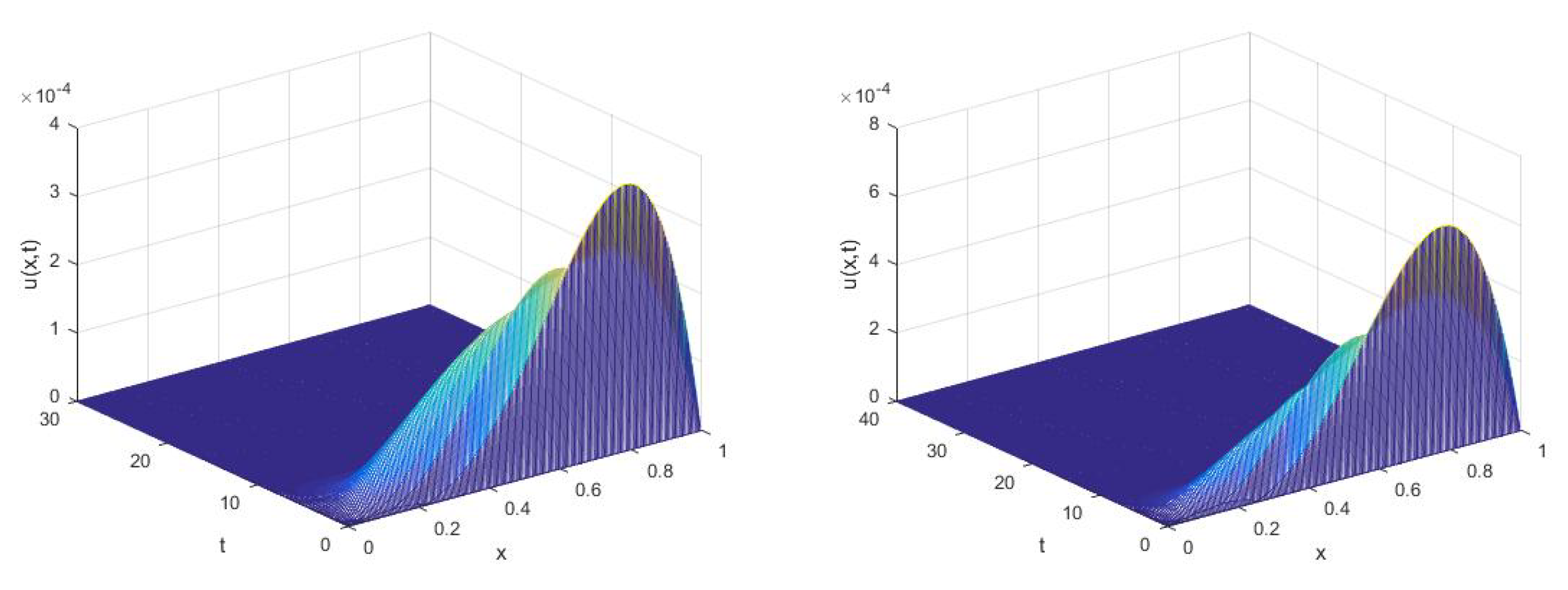
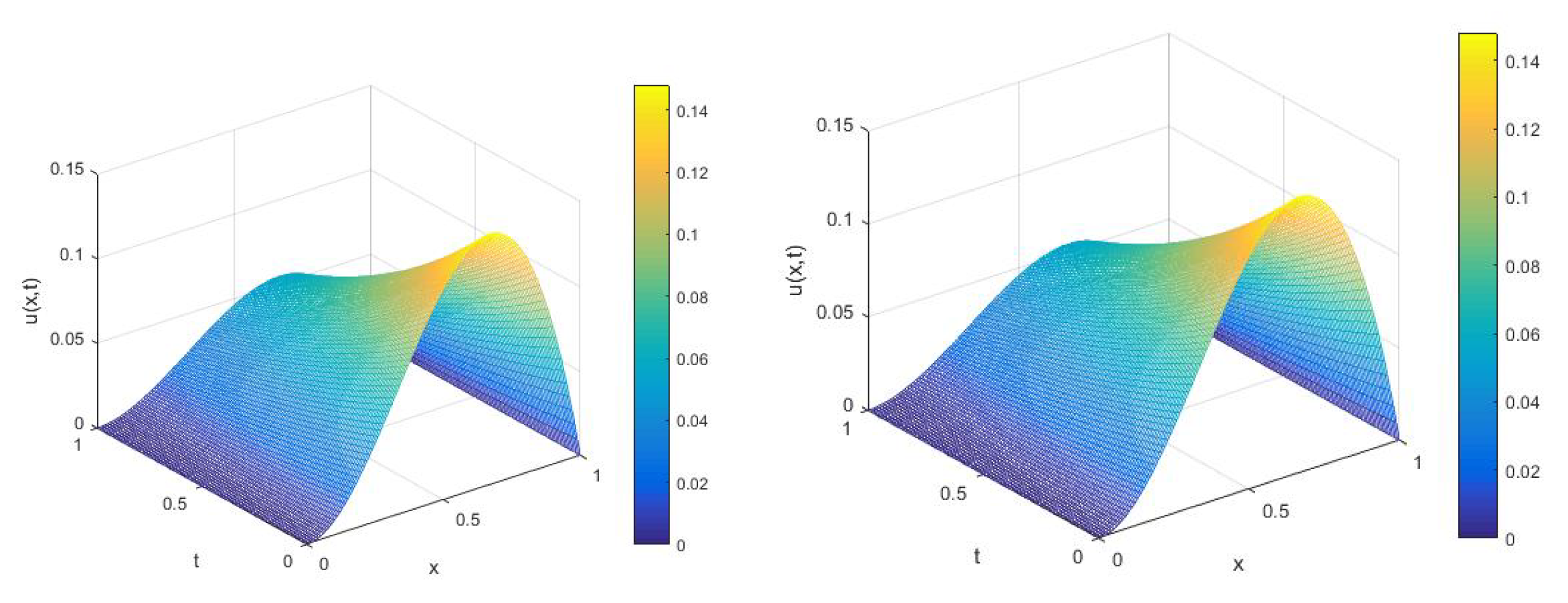
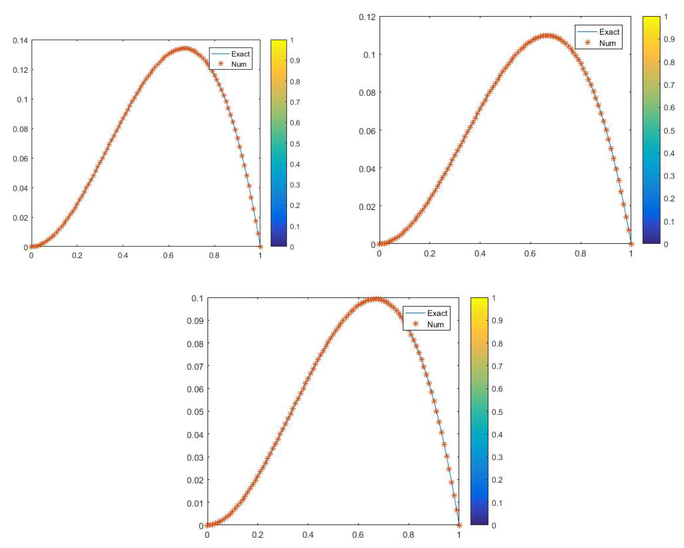
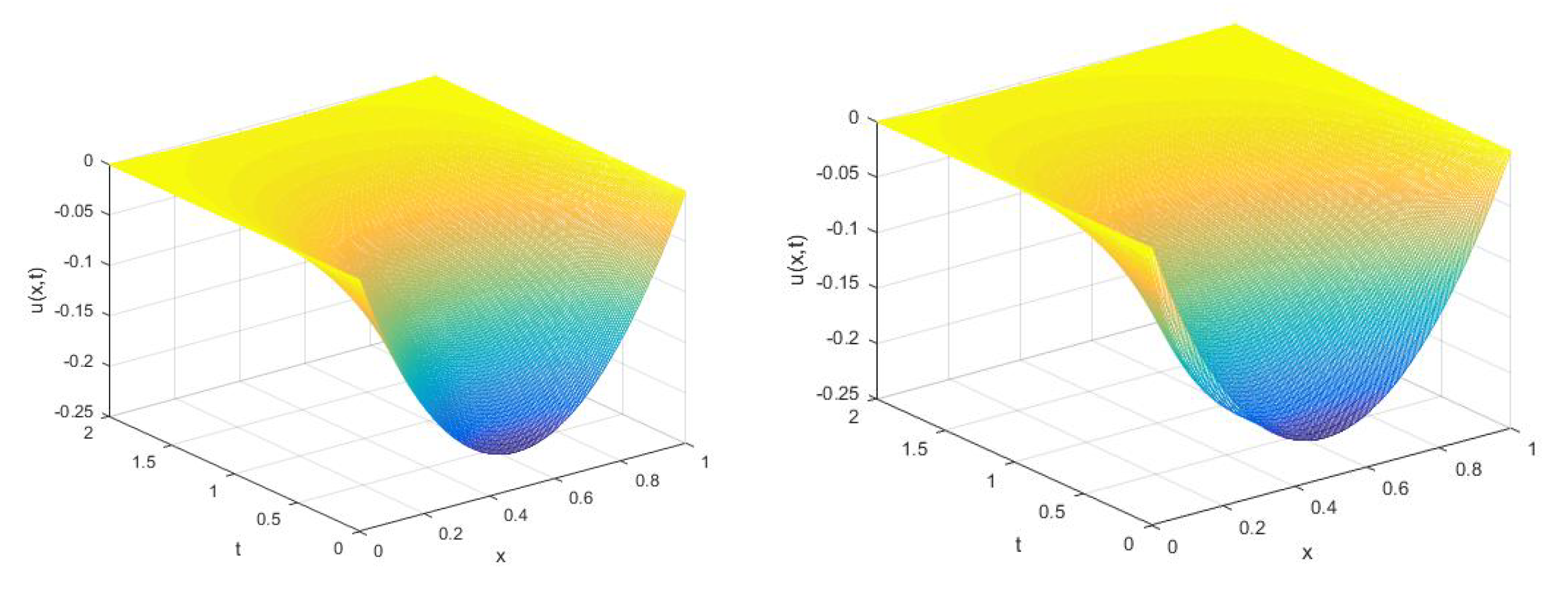
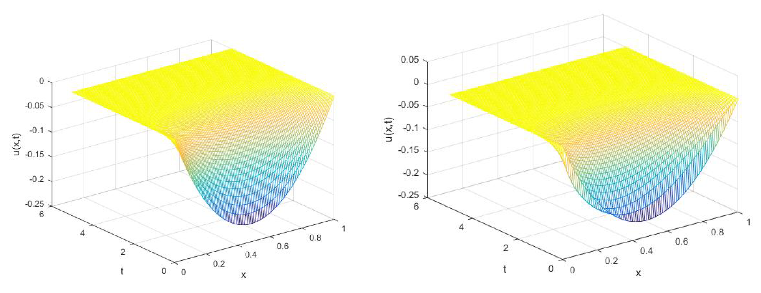
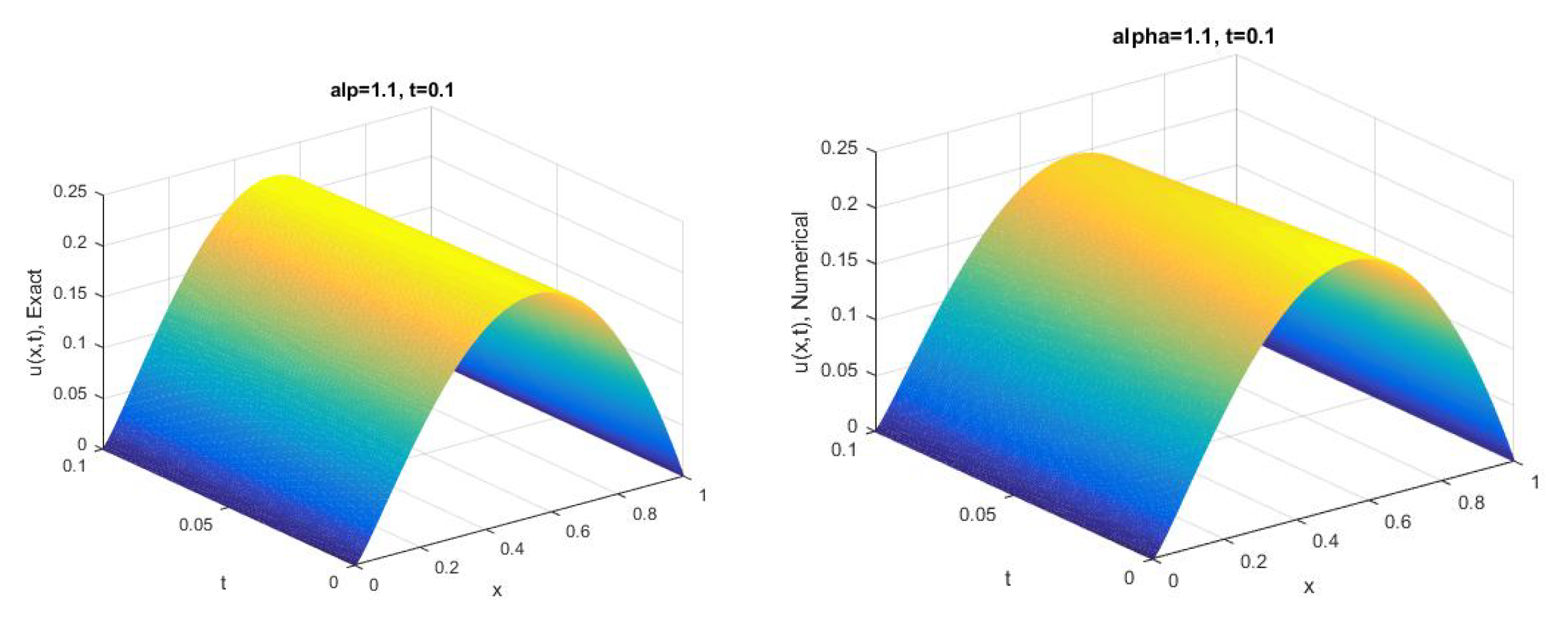
First of all we have given the Truncation error of the C-N scheme. It is obvious to conclude that:

$$\begin{array}{ccc}\hfill {\displaystyle \frac{u(x_m,t_{n+1})-u(x_m,t_n)}{\tau }}& =& {\left({\displaystyle \frac{\partial u(x,t)}{\partial t}}\right)}^{n+1/2}+O\left({\tau }^2\right).\hfill \\ \hfill {\left(c\left(x\right){\displaystyle \frac{\partial u(x,t)}{\partial x}}+d\left(x\right){\displaystyle \frac{{\partial }^{\alpha }u(x,t)}{\partial x^{\alpha }}}\right)}_m^{n+1/2}& =& \frac{1}{2}\left(c_m{\displaystyle \frac{\partial u(x_m,t_{n+1})}{\partial x}}+d_m{\displaystyle \frac{{\partial }^{\alpha }u(x_m,t_{n+1}}{\partial x^{\alpha }}}\right)\hfill \\ & +& \frac{1}{2}\left(c_m{\displaystyle \frac{\partial u(x_m,t_n)}{\partial x}}+d_m{\displaystyle \frac{{\partial }^{\alpha }u(x_m,t_n}{\partial x^{\alpha }}}\right)+O\left({\tau }^2\right).\hfill \end{array}$$

(36)

$$c\left(x_m\right){\displaystyle \frac{\partial u(x,t)}{\partial x}}\approx {\displaystyle \frac{u(x_{m+1},t_{n+1})-u(x_{m-1},t_{n+1})}{2h}}+O\left(h^2\right).$$

(37)

From the above Extrapolation to the limit Theorem for $n=1$, we got

$${\displaystyle \frac{{\partial }^{\alpha }u(x,t)}{\partial x^{\alpha }}}\approx \sum _{k=0}^{m+1}{g}_k^{\left(\alpha \right)}{u}_{m-k+1}+O\left(h^2\right).$$

(38)

Therefore the local truncation error of (20) is given by $T_m^{n+1}=O({\tau }^2+\tau h)$

Theorem 5.

Let $u_m^n$ be the exact solution of problem (20), and $U_m^n$ be the solution of the finite difference scheme (26), then for all $1\le n\le N_t$, we have the estimate

$${∥u_m^n-U_m^n∥}_{\infty }\le c({\tau }^2+h)$$

where ${∥u_m^n-U_m^n∥}_{\infty }$=$ma{x}_{1\le m\le N_x}\left|u_m^n-U_m^n\right|$, c is a non-negative constant independent of h and τ with $\left|\right|.\left|\right|$ stands for the discrete $L^2$-norm.

Proof of Theorem 5.

Denote $e^n=u_m^n-U_m^n$ where $e^n=(e_1^n,e_2^n,\dots ,e_{N_x-1}^n)$. We have $e^0=0$, we have from Equations (26) and (27) if $n=0$,

$$\begin{array}{ccc}\hfill R_m^1& =& \left({\displaystyle \frac{-{\mu }_m}{2}}-{\displaystyle \frac{{\eta }_m}{2}}{\omega }_0^{\left(\alpha \right)}\right)e_{m-1}^1+\left(1+{\displaystyle \frac{{\eta }_m}{2}}\alpha \right)e_1^m\hfill \\ & +& \left({\displaystyle \frac{-{\mu }_m}{2}}-{\displaystyle \frac{{\eta }_m}{2}}{\omega }_2^{\left(\alpha \right)}\right)e_{m+1}^1-{\displaystyle \frac{{\eta }_m}{2}}\sum _{k=3}^{N_x}{\omega }_k^{\left(\alpha \right)}{e}_{m-n+1}^1.\hfill \end{array}$$

if $n>0$,

$$\begin{array}{ccc}\hfill R_m^{n+1}& =& \left({\displaystyle \frac{-{\mu }_m}{2}}-{\displaystyle \frac{{\eta }_m}{2}}{\omega }_0^{\left(\alpha \right)}\right)e_{m-1}^{n+1}+\left(1+{\displaystyle \frac{{\eta }_m}{2}}\alpha \right)e_{n+1}^m\hfill \\ & +& \left({\displaystyle \frac{-{\mu }_m}{2}}-{\displaystyle \frac{{\eta }_m}{2}}{\omega }_2^{\left(\alpha \right)}\right)e_{m+1}^{n+1}-{\displaystyle \frac{{\eta }_m}{2}}\sum _{k=3}^{N_x}{\omega }_k^{\left(\alpha \right)}{e}_{m-n+1}^{n+1}.\hfill \end{array}$$

where $R_m^{n+1}\le c({\tau }^2+h),m=1,2,\dots ,N_x-1,n=1,2,3,\dots ,N_t-1$, c is non-negative constant independent of h and $\tau$.

We can use the mathematical induction to prove the Theorem. Let $n=1$ and assume $|e_j|=ma{x}_{1\le m\le N_x-1}\left|e_m^1\right|$, we have the following expression.

$$\begin{array}{ccc}\hfill \left|\right|e^1{\left|\right|}_{\infty }& =& \left|e_j^1\right|\le \left({\displaystyle \frac{-{\mu }_j}{2}}-{\displaystyle \frac{{\eta }_j}{2}}{\omega }_0^{\left(\alpha \right)}\right)\left|e_{j-1}^1\right|+\left(1+{\displaystyle \frac{{\eta }_j}{2}}\alpha \right)\left|e_1^j\right|\hfill \\ & +& \left({\displaystyle \frac{-{\mu }_j}{2}}-{\displaystyle \frac{{\eta }_j}{2}}{\omega }_2^{\left(\alpha \right)}\right)\left|e_{j+1}^1\right|-{\displaystyle \frac{{\eta }_j}{2}}\sum _{k=3}^{N_x}{\omega }_k^{\left(\alpha \right)}\left|e_{j-n+1}^1\right|\hfill \\ & \le & \left|\left({\displaystyle \frac{-{\mu }_j}{2}}-{\displaystyle \frac{{\eta }_j}{2}}{\omega }_0^{\left(\alpha \right)}\right)e_{j-1}^1+\left(1+{\displaystyle \frac{{\eta }_j}{2}}\alpha \right)e_1^j+\left({\displaystyle \frac{-{\mu }_j}{2}}-{\displaystyle \frac{{\eta }_j}{2}}{\omega }_2^{\left(\alpha \right)}\right)e_{j+1}^1-{\displaystyle \frac{{\eta }_j}{2}}\sum _{k=3}^{N_x}{\omega }_k^{\left(\alpha \right)}{e}_{j-n+1}^1\right|\hfill \\ & =& \left|R_j^1\right|\le c({\tau }^2+h).\hfill \end{array}$$

Suppose that if $n\le r,\left|\right|e^r{\left|\right|}_{\infty }\le c({\tau }^2+h^2)$ hold and assume $n=r+1$, let $\left|e_j^{r+1}\right|=ma{x}_{1\le m\le N_x-1}\left|e_m^{r+1}\right|$, notice that from Lemma 1, we have ${\sum }_{k=0}^{N_x}{\omega }_k^{\left(\alpha \right)}<0,m=1,2,\dots ,N_x$. Therefore,

$$\begin{array}{ccc}\hfill {∥e^{r+1}∥}_{\infty }& =& \left|e_j^{r+1}\right|\le \left({\displaystyle \frac{-{\mu }_j}{2}}-{\displaystyle \frac{{\eta }_j}{2}}{\omega }_0^{\left(\alpha \right)}\right)\left|e_{j-1}^{r+1}\right|+\left(1+{\displaystyle \frac{{\eta }_j}{2}}\alpha \right)\left|e_{r+1}^j\right|\hfill \\ & +& \left({\displaystyle \frac{-{\mu }_j}{2}}-{\displaystyle \frac{{\eta }_j}{2}}{\omega }_2^{\left(\alpha \right)}\right)\left|e_{j+1}^{r+1}\right|-{\displaystyle \frac{{\eta }_j}{2}}\sum _{k=3}^{N_x}{\omega }_k^{\left(\alpha \right)}\left|e_{j-n+1}^{r+1}\right|\hfill \\ & \le & \left|\left({\displaystyle \frac{-{\mu }_j}{2}}-{\displaystyle \frac{{\eta }_j}{2}}{\omega }_0^{\left(\alpha \right)}\right)e_{j-1}^{r+1}+\left(1+{\displaystyle \frac{{\eta }_j}{2}}\alpha \right)e_{r+1}^j+\left({\displaystyle \frac{-{\mu }_j}{2}}-{\displaystyle \frac{{\eta }_j}{2}}{\omega }_2^{\left(\alpha \right)}\right)e_{j+1}^{r+1}-{\displaystyle \frac{{\eta }_j}{2}}\sum _{k=3}^{N_x}{\omega }_k^{\left(\alpha \right)}{e}_{j-n+1}^{r+1}\right|\hfill \\ & =& \left|R_j^{r+1}\right|\le c({\tau }^2+h)\hfill \end{array}$$

which completes the proof. □

Remark 3.

The Crank–Nicolson scheme, for classical convection–diffusion equation, provides stable C-N finite difference method that is second order convergence in time and space. Also a study based on C-N finite difference method with the spatial extrapolation to the limit method, see Theorem 1, is used to get temporal and spatial second order for one-sided SFCDEs with space variable coefficients.

5. Numerical Tests

Problem test 1

1. Consider the space-fractional diffusion type of problem:

$$\frac{\partial u(x,t)}{\partial t}=d\left(x\right)\frac{{\partial }^{\alpha }u(x,t)}{\partial x^{\alpha }}+p(x,t)$$

with initial condition

$$u(x,0)=(x^2-x^3);0\le x\le 1$$

homogeneous Dirichlet boundary condition

$$u(0,t)=0=u(1,t)$$

with variable diffusion coefficient,

$$d\left(x\right)=\mathsf{\Gamma }\left(1.2\right)x^{\alpha },$$

and source term

$$p(x,t)=(6x^3-3x^2)e^{-t}$$

The exact solution is

$$u(x,t)=(x^2-x^3)e^{-t}$$

All numerical experiments are implemented using Theorem 1 and C-N scheme with the space domain, $0<x<1$ and time domain, $0<t<T$. Figure 1 shows the maximum error produced by C-N scheme for large enough time domain and numerical solution is close enough to the exact solution using C-N scheme with $\alpha =1.5$ in Figure 2. The maximum error and second order convergence for the fractional diffusion and fractional convection–diffusion equation with variable coefficients are given in

Table 1. The maximum error and convergence order of the C-N scheme for FDE in example 1.

		$\mathit{\alpha }=1.25$		$\mathit{\alpha }=1.5$		$\mathit{\alpha }=1.8$
$\mathsf{\Delta }\mathit{t}$	$\mathsf{\Delta }\mathit{x}$	Max-Error	Order	Max-Error	Order	Max-Error	Order
1/50	1/50	4.9807e−04	–	4.0046e−04	–	1.4048e−04	–
1/100	1/100	1.0660e−04	2.2241	8.8946e−05	2.1707	3.6848e−05	1.9307
1/200	1/200	2.4413e−05	2.1265	2.0643e−05	2.1073	9.4393e−06	1.9648
1/400	1/400	5.8239e−06	2.0676	4.9592e−06	2.0575	2.3887e−06	1.9825
1/800	1/800	1.4211e−06	2.0350	1.2146e−06	2.0296	6.0078e−07	1.9913

,

Table 2. The maximum error and convergence order for FCDE in example 2.

		$\mathit{T}=1$		$\mathit{T}=5$
$\mathsf{\Delta }\mathit{t}$	$\mathsf{\Delta }\mathit{x}$	Max-Error	Order	Max-Error	Order
1/50	1/50	1.4048e−04	–	2.5297e−05	–
1/100	1/100	3.6848e−05	1.9307	7.4748e−06	1.7589
1/200	1/200	9.4393e−06	1.9648	2.0122e−06	1.8933
1/400	1/400	2.3887e−06	1.9825	4.9017e−07	2.0374
1/800	1/800	6.0078e−07	1.9913	1.0620e−07	2.2065

and

Table 3. The maximum error and convergence order by C-N for SFCDE in example 2 at $T=1,\alpha =1.55$.

$\mathsf{\Delta }\mathit{t}$	$\mathsf{\Delta }\mathit{x}$	Max-Error	Order
1/50	1/50	2.6e−03	–
1/100	1/100	7.695e−04	1.7563
1/150	1/150	2.144e−04	1.8436
1/200	1/200	5.688e−05	1.9143

.

Problem test 2

2. Consider the space-fractional convection–diffusion type of equation with variable coefficients:

$$\frac{\partial u(x,t)}{\partial t}+c\left(x\right)\frac{\partial u(x,t)}{\partial x}=d\left(x\right)\frac{{\partial }^{\alpha }u(x,t)}{\partial x^{\alpha }}+p(x,t)$$

with initial condition

$$u(x,0)=(x^{\alpha }-x);0\le x\le 1$$

homogeneous Dirichlet boundary condition

$$u(0,t)=0=u(1,t)$$

with variable convection–diffusion coefficients respectively,

$$c\left(x\right)=x^{\frac{1}{5}},d\left(x\right)=x^{\frac{1}{100}},$$

and source term

$$p(x,t)=e^{-2t}(2(x-x^{\alpha })-\mathsf{\Gamma }\left(\alpha \right)+\frac{\mathsf{\Gamma }(\alpha +1)}{\mathsf{\Gamma }\left(\alpha \right)}{x}^{\alpha -1}-1)$$

The exact solution is

$$u(x,t)=e^{-2t}(x^{\alpha }-x)$$

Figure 3 and Figure 4 show the numerical and exact solutions for fractional diffusion and fractional convection–diffusion problems with large enough time domain in example 1 and 2, respectively.The exact and numerical solution of fractional convection–diffusion equation by C-N scheme is also given in Figure 5. In

Table 4. The Maximum error and convergence order produced by C-N scheme for example 3 at $T=1,N_t=100$.

		$\mathit{\alpha }=1.35$		$\mathit{\alpha }=1.5$		$\mathit{\alpha }=1.75$
$\mathsf{\Delta }\mathit{x}$	Max-Error	Order	Max-Error	Order	Max-Error	Order
1/50	4.5e−03	–	2.8e−03	–	1.7e−03	–
1/100	2.7e−03	0.7370	1.6e−03	0.8074	8.9641–04	0.97224
1/200	1.6e−03	0.7549	8.6405e−04	0.8889	4.6491e−04	0.8981
1/400	9.5896e−04	0.7385	4.7955e−04	0.8494	2.4086e−04	0.9488
1/800	5.7034e−04	0.7496	2.6609e−04	0.8498	1.2473e−04	0.9494

, the maximum error and first order convergence in space is obtained using C-N scheme without extrapolation to the limit approach by fixing the time step.

Problem Test 3

3. Consider the space-fractional convection–diffusion type of equation with variable coefficients:

$$\frac{\partial u(x,t)}{\partial t}+c\left(x\right)\frac{\partial u(x,t)}{\partial x}=d\left(x\right)\frac{{\partial }^{\alpha }u(x,t)}{\partial x^{\alpha }}+p(x,t)$$

with initial condition

$$u(x,0)=x^2(1-x)$$

homogeneous Dirichlet boundary condition

$$u(0,t)=0=u(1,t)$$

with variable convection–diffusion coefficients respectively,

$$c\left(x\right)=x^{0.6},d\left(x\right)=\mathsf{\Gamma }\left(2.8\right)x^{3/4}$$

and the forcing function

$$p(x,t)=2x^2(1-x)t^{1.3}/\mathsf{\Gamma }\left(2.3\right)+0.3x^{1.8}{e}^{-t}$$

The exact solution is

$$u(x,t)=x^2(1-x)e^{-t}$$

Problem test 4

4. Consider the space-fractional convection–diffusion equation with variable coefficients:

$$\frac{\partial u(x,t)}{\partial t}+c\left(x\right)\frac{\partial u(x,t)}{\partial x}=d\left(x\right)\frac{{\partial }^{\alpha }u(x,t)}{\partial x^{\alpha }}+p(x,t)$$

with initial condition

$$u(x,0)=x^{\alpha }(1-x)$$

homogeneous Dirichlet boundary condition

$$u(0,t)=0=u(1,t)$$

with variable convection–diffusion coefficients respectively,

$$c\left(x\right)=x^{3/5},d\left(x\right)=x^{3/4}$$

and the forcing function

$$p(x,t)=2x^{\alpha }(1-x)t^{1.3}/\mathsf{\Gamma }\left(2.3\right)+0.3x^{1.8}{e}^{-t}$$

The exact solution is

$$u(x,t)=x^{\alpha }(1-x)e^{-t}$$

Problem test 4 is experimented with the grid size reduction extrapolation approach stated in [23]. We have smooth enough numerical and exact solutions by using C-N scheme in Figure 6, and

Table 5. The Maximum error and error-rate produced by C-N scheme for example 4 at $t=0.1$.

		$\mathit{\alpha }=1.25$		$\mathit{\alpha }=1.55$
$\mathsf{\Delta }\mathit{t}$	$\mathsf{\Delta }\mathit{x}$	Max-Error	Error-Rate	Max-Error	Error-Rate
1/50	1/50	1.91e−02	–	1.52e−02	–
1/100	1/100	9.9e−03	1.93	7.9e−03	1.9
1/200	1/200	5.2e−03	1.90	4.3e−03	1.84
1/400	1/400	2.8e−03	1.86	2.4e−03	1.79
1/800	1/800	1.6e−03	1.75	1.4e−03	1.7

shows the maximum error with the error rate is given for space fractional convection–diffusion problem with a grid size reduction extrapolation method.

6. Conclusions

The one dimension space fractional diffusion and fractional convection–diffusion problem with space variable coefficients is solved by the fractional C-N scheme based on the Extrapolation to the limit approach of right shifted Grünwald–Letnikov approximation. The fractional C-N method, for the fractional diffusion problem and fractional convection–diffusion equation with space variable coefficients, is consistent and unconditionally stable with second order convergence. Numerical examples confirmed that the C-N method is suitable for the space fractional convection–diffusion problem even for a large value of time domain.

References

1. Diethelm, K. The Analysis of Fractional Differential Equations; Springer Science & Business Media: Berlin/Heidelberg, Germany, 2010. [Google Scholar]
2. Fomin, S.; Chugunov, V.; Hashida, T. Application of fractional differential equations for modeling the anomalous diffusion of contaminant from fracture into porous rock matrix with bordering alteration zone. Trans. Porous Med. 2010, 81, 187–205. [Google Scholar] [CrossRef]
3. Guo, B.; Pu, X.; Huang, F. Fractional Partial Differential Equations and Their Numerical Solutions; World Scientific: Singapore, 2015. [Google Scholar]
4. Podlubny, I. Fractional Differential Equations Academic; Academic Press: New York, NY, USA, 1999. [Google Scholar]
5. Podlubny, I. Fractional Differential Equations: An Introduction to Fractional Derivatives, Fractional Differential Equations, to Methods of Their Solution and Some of Their Applications; Elsevier: New York, NY, USA, 1998; Volume 198. [Google Scholar]
6. Salman, W.; Gavriilidis, A.; Angeli, P. A model for predicting axial mixing during gas–liquid Taylor flow in microchannels at low Bodenstein number. Chem. Eng. J. 2004, 101, 391–396. [Google Scholar] [CrossRef]
7. Berkowitz, B.; Cortis, A.; Dror, I.; Scher, H. Laboratory experiments on dispersive transport across interfaces. Water Resour. Res. 2009, 45. [Google Scholar] [CrossRef] [Green Version]
8. Cortis, A.; Berkowitz, B. Computing “anomalous” contaminant transport in porous media. Ground Water 2005, 43, 947–950. [Google Scholar] [CrossRef]
9. Meerschaert, M.M.; Tadjeran, C. Finite difference approximations for fractional advection–dispersion flow equations. J. Comput. Appl. Math. 2004, 172, 65–77. [Google Scholar] [CrossRef] [Green Version]
10. Meerschaert, M.M.; Tadjeran, C. Finite difference approximations for two-sided space fractional partial differential equations. Appl. Numer. Math. 2006, 56, 80–90. [Google Scholar] [CrossRef]
11. Ren, J.; Sun, Z.Z.; Zhao, X. Compact difference scheme for the fractional sub-diffusion equation with Neumann boundary conditions. J. Comput. Phys. 2013, 232, 456–467. [Google Scholar] [CrossRef]
12. Wang, K.; Wang, H. A fast characteristic finite difference method for fractional advection–diffusion equations. Adv. Water. Resour. 2011, 34, 810–816. [Google Scholar] [CrossRef]
13. Singh, J.; Swroop, R.; Kumar, D. A computational approach for fractional convection–diffusion equation via integral transforms. Ain Shams Eng. J. 2016, 9, 1019–1028. [Google Scholar] [CrossRef] [Green Version]
14. Liu, F.; Zhuang, P.; Burrage, K. Numerical methods and analysis for a class of fractional advection–dispersion models. Comput. Math. Appl. 2012, 64, 2990–3007. [Google Scholar] [CrossRef] [Green Version]
15. Tian, W.; Deng, W.; Wu, Y. Polynomial spectral collocation method for space fractional advection–diffusion equation. Numer. Methods Partial Differ. Equ. 2014, 30, 514–535. [Google Scholar] [CrossRef] [Green Version]
16. Hejazi, H.; Moroney, T.; Liu, F. Comparison of finite difference and finite volume methods for solving the space fractional advection–dispersion equation with variable coefficients. ANZIAM J. 2013, 54, 557–573. [Google Scholar] [CrossRef] [Green Version]
17. Liu, F.; Zhuang, P.; Turner, I.; Burrage, K.; Anh, V. A new fractional finite volume method for solving the fractional diffusion equation. Appl. Math. Model. 2014, 38, 15–16. [Google Scholar] [CrossRef]
18. Li, C.; Zeng, F. Numerical Methods for Fractional Calculus; Chapman and Hall/CRC: Boca Raton, FL, USA, 2015. [Google Scholar]
19. Li, C.; Zeng, F. Finite difference methods for fractional differential equations. Int. J. Bifurcat. Chaos 2012, 22, 1230014. [Google Scholar] [CrossRef]
20. Luchko, Y. Multi-dimensional fractional wave equation and some properties of its fundamental solution. Ind. Math. 2014, 6. [Google Scholar] [CrossRef]
21. Lynch, V.E.; Carreras, B.A.; del-Castillo-Negrete, D.; Ferreira-Mejias, K.M.; Hicks, H.R. Numerical methods for the solution of partial differential equations of fractional order. J. Comput. Phys. 2003, 192, 406–421. [Google Scholar] [CrossRef]
22. Sweilam, N.H.; Khader, M.M.; Mahdy, A.M.S. Crank–Nicolson finite difference method for solving time-fractional diffusion equation. J. Fract. Calc. Appl. 2012, 2, 1–9. [Google Scholar]
23. Tadjeran, C.; Meerschaert, M.M.; Scheffler, H.P. A second-order accurate numerical approximation for the fractional diffusion equation. J. Comput. Phys. 2006, 201, 205–213. [Google Scholar] [CrossRef]
24. Wang, Y.M. A compact finite difference method for a class of time fractional convection–diffusion-wave equations with variable coefficients. Num. Algor. 2015, 70, 625–651. [Google Scholar] [CrossRef]
25. Wang, Y.M.; Wang, T. A compact Alternative difference implicit method and its extrapolation for time fractional sub-diffusion equations with nonhomogeneous Neumann boundary conditions. Comput. Math. Appl. 2018, 75, 721–739. [Google Scholar] [CrossRef]
26. Zhou, F.; Xu, X. The third kind Chebyshev wavelets collocation method for solving the time-fractional convection–diffusion equations with variable coefficients. Appl. Math. Comput. 2016, 280, 11–29. [Google Scholar] [CrossRef]
27. Jin, B.; Lazarov, R.; Zhou, Z. A Petrov–Galerkin finite element method for fractional convection–diffusion equations. SIAM J. Numer. Anal. 2016, 54, 481–503. [Google Scholar] [CrossRef] [Green Version]
28. Gao, F.; Yuan, Y.; Du, N. An upwind finite volume element method for nonlinear convection–diffusion problem. AJCM 2011, 1, 264. [Google Scholar] [CrossRef] [Green Version]
29. Aboelenen, T. A direct discontinuous Galerkin method for fractional convection–diffusion and Schrödinger-type equations. Eur. Phys. J. Plus 2018, 133, 316. [Google Scholar] [CrossRef]
30. Xu, Q.; Hesthaven, J.S. Discontinuous Galerkin method for fractional convection–diffusion equations. SIAM J. Numer. Anal. 2014, 52, 405–423. [Google Scholar] [CrossRef] [Green Version]
31. Bhrawy, A.H.; Baleanu, D. A spectral Legendre−Gauss–Lobatto collocation method for a space-fractional advection–diffusion equations with variable coefficients. Rep. Math. Phys. 2013, 72, 219–233. [Google Scholar] [CrossRef]
32. Saadatmandi, A.; Dehghan, M.; Azizi, M.R. The Sinc-Legendre collocation method for a class of fractional convection–diffusion equations with variable coefficients. Commun. Nonlinear. Sci. Numer. Simulat. 2012, 17, 4125–4136. [Google Scholar] [CrossRef]
33. Pang, G.; Chen, W.; Sze, K.Y. A comparative study of finite element and finite difference methods for two-dimensional space-fractional advection–dispersion equation. Adv. Appl. Math. Mech. 2016, 8, 166–186. [Google Scholar] [CrossRef]
34. Zhang, Y. A finite difference method for fractional partial differential equation. Appl. Math. Comput. 2009, 2015, 524–529. [Google Scholar] [CrossRef]
35. Gu, X.M.; Huang, T.Z.; Ji, C.C. Carpentieri B, Alikhanov AA, Fast iterative method with a second-order implicit difference scheme for time-space fractional convection–diffusion equation. J. Sci. Comput. 2017, 72, 957–985. [Google Scholar] [CrossRef]
36. Benson, D.A.; Wheatcraft, S.; Meerschaert, M.M. Application of a fractional advection–dispersion equation. Water Resour. Res. 2000, 36, 1403–1412. [Google Scholar] [CrossRef] [Green Version]
37. Tian, W.; Zhou, H.; Deng, W. A class of second order difference approximations for solving space fractional diffusion equations. Math. Comp. 2015, 84, 1703–1727. [Google Scholar] [CrossRef] [Green Version]
38. Henrici, P. Elements of Numerical Analysis; John Wiley and Sons: New York, NY, USA, 1984. [Google Scholar]
39. Tuan, V.K.; Gorenflo, R. Extrapolation to the Limit for Numerical Fractional Differentiation. Z. Angew. Math. Mech. 1995, 75, 646–648. [Google Scholar] [CrossRef]
40. LeVeque, R.J. Finite Difference Methods for Ordinary and Partial Differential Equations; SIAM: Philadelphia, PA, USA, 2007; Volume 98. [Google Scholar]
41. Isaacson, E.; Keller, H.B. Analysis of Numerical Methods; Courier Corporation: Chelmsford, MA, USA, 2012. [Google Scholar]
Figure 1. The Maximum error by C-N scheme at ( T = 10 , M a x E r r o r = 6.5276 e 07 ) , ( T = 20 , M a x E r r o r = 1.7244 e 08 ) , α = 1.5 left to right, respectively, for Example 1.
Symmetry 12 00485 g001
Figure 2. The exact (left) and numerical (right) solution by C-N scheme at T = 1 , α = 1.5 , τ = 0.01 = h for Example 1.
Symmetry 12 00485 g002
Figure 3. Numerical and exact solution by C-N scheme at α = 1.5 , τ = h = 0.01 , with ( T = 10 , T = 30 , T = 40 ) left to right-down respectively, for Example 1.
Symmetry 12 00485 g003
Figure 4. The exact (left) and numerical (right) solution by C-N scheme for the FCDE at ( h = τ = 0.005 , α = 1.5 , ( t = 5 , max e r r o r = 4.0657 e 05 ) for Example 2.
Symmetry 12 00485 g004
Figure 5. The exact (left) and numerical (right) solution by C-N scheme for the FCDE at ( h = τ = 0.01 , ( t = 2 , max E r r o r = 4.2158 e 04 ) , α = 1.75 ) for Example 2.
Symmetry 12 00485 g005
Figure 6. The exact (left) and numerical (right) solution by C-N scheme at ( h = τ = 0.0025 , ( t = 0.1 , max E r r o r = 1.4 e 03 , α = 1.1 ) for Example 4.
Symmetry 12 00485 g006