Improving the Results of the Earned Value Management Technique Using Artificial Neural Networks in Construction Projects

Abstract

The cost, time and scope of a construction project are key parameters for its success. Thus, predicting these indices is indispensable. Correct and accurate prediction of cost throughout the progress of a project gives project managers the chance to identify projects that need revision in their schedules in order to result in the maximum benefit. The aim of this study is to minimize the shortcomings of the Earned Value Management (EVM) method using an Artificial Neural Network (ANN) and multiple regression analysis in order to predict project cost indices more precisely. A total of 50 road construction projects in Fars Province, Iran, were selected for analysis in this research. An ANN model was used to predict the projects’ cost performance indices, thereby creating a more accurate symmetry between the predicted and actual cost by considering factors that influence project success. The input data of the ANN model were analysed in MATLAB software. A multiple regression model was also used as another analytical tool to validate the outcome of the ANN. The results showed that the ANN model resulted in a lower Mean Squared Error (MSE) and a greater correlation coefficient than both the traditional EVM model and the multiple regression model.

1. Introduction

The number of road construction projects is increasing dramatically every year. Although project management is being more expertly implemented, there are still problems associated with cost overruns in projects [1]. One of the factors that increases the capital output ratio for a country’s economy is cost overrun. Estimating the cost of projects has always been a crucial, demanding and sophisticated challenge [2,3]. Cost estimation is a process in which the total cost of a project is predicted based on the existing information [4]. Generally, cost estimation is conducted in order to set the initial budget of a project, which will ideally produce symmetry between the initial estimation and the subsequent actual cost [1]. Cost estimation presents some difficulties, such as the initial information required, the small number of databases available for road construction project costs, the low efficiency of existing cost estimation methods and the existence of uncertainties [5].

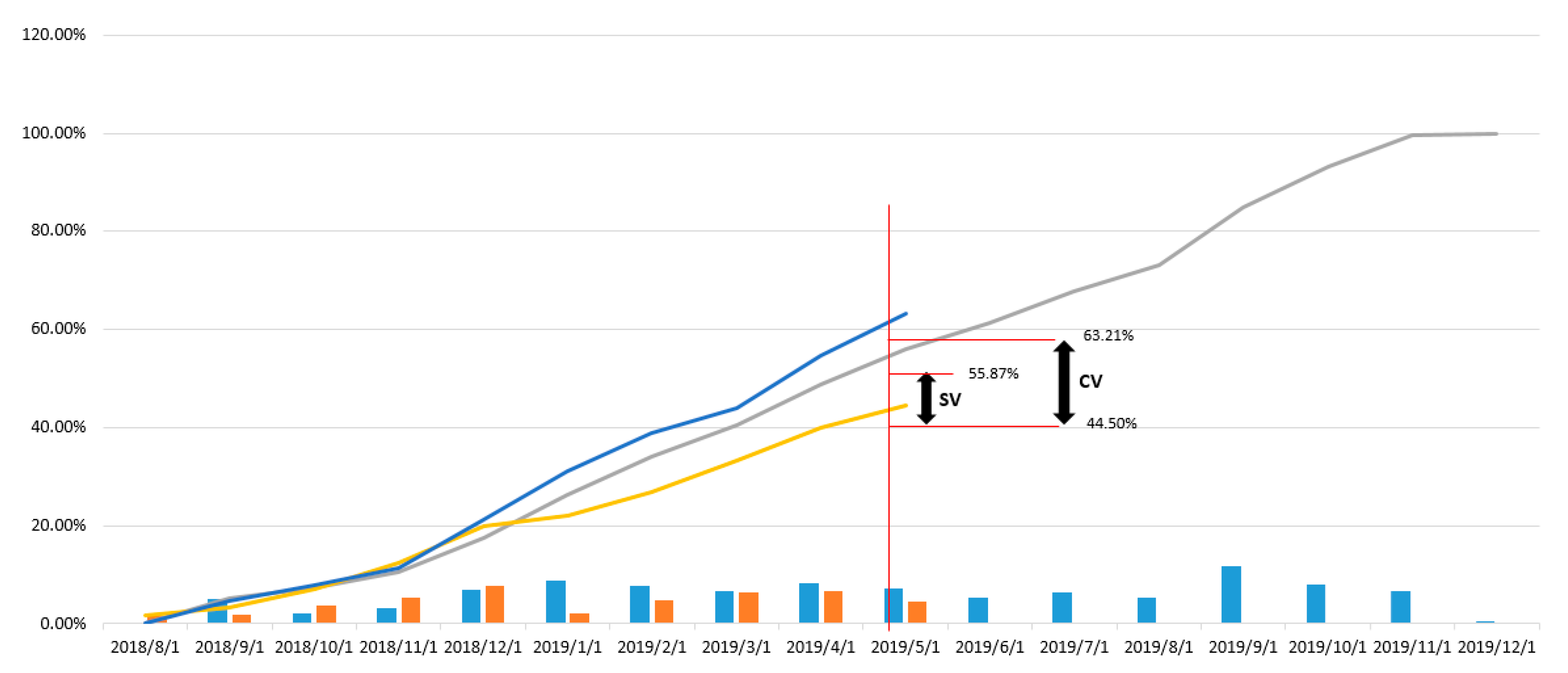
Earned Value Management (EVM) is a tool to help with controlling the progress of a project. EVM is able to illustrate the current status of projects, as well as measuring current variances [6]. To assess the progress of projects, EVM exploits three constraints: time, scope and cost. Moreover, EVM is able to predict the future parameters of projects, including the final cost, based on existing data [7,8,9]. This comprehensive management approach has been widely used in numerous studies and in different fields [10,11,12,13,14].

Artificial Neural Networks (ANNs) are an effective tool that imitates the human mind for application in various problems [15]. The first application of ANNs in construction activities took place in the late 1980s [16]. Adeli (2001) published the first scientific article regarding the use of ANNs in the construction industry [17]. ANNs are widely used in various stages of a project, including design, construction, maintenance, renovation and destruction [18]. Some examples of the use of ANNs are presented in the following.

Albino and Garavelli (1998) applied a neural network in order to rank subcontractors in construction firms [19]. Leung et al. (2001) exploited ANNs to predict the hoisting times of tower cranes [20]. Cheung et al. (2006) forecasted the performance of projects using neural networks [21]. Vouk et al. (2011) analyzed the economy of wastewater systems using neural networks [22]. Mucenski et al. (2013) estimated the recycling capacity of multistorey buildings using ANNs [23]. Chaphalkar et al. (2015) used a multilayer perceptron neural network in order to forecast the outcome of construction dispute claims [24]. Golanaraghi et al. (2019) predicted formwork labor productivity using an ANN [25]. Tijanic et al. (2019) used an ANN in order to predict costs in road construction [26]. Readers are referred to References [27,28,29,30,31,32,33,34,35,36] for further uses of ANNs for various applications in the construction industry, as well as in other fields of science.

Cost, time and quality are the three components of success in a construction project. In other words, a project in which construction is finished within the predicted cost, to the required quality and within the forecasted time can be called a successful project [37]. The cost of construction projects usually deviates from the initial estimation due to a variety of factors [38]. In other words, the costs in construction projects do not usually remain the same as they were predicted to be before the construction phase. Cost increases are normal, as can be seen in most projects [39]. According to the available literature, not many projects are finished within the forecasted cost. A lot of construction projects face both delays and cost overruns [40]. Flyvbejerg et al. illustrated that cost underestimation happens dramatically more frequently than cost overestimation [41]. Iran is a developing country, and cost overruns are common in such countries. For instance, Heravi and Mohammadian (2019) investigated 72 construction projects in Iran based on both their documentation and their actual performance. They concluded that larger projects faced higher cost overruns and delays [42]. Although EVM is able to illustrate the degree to which delays and cost shortages exist in a project on the basis of the project’s previous data, it cannot provide an accurate prediction of the future status of the project [8,9].

EVM results are obtained during and after the implementation phase. Thus, having the ability to predict the future situation of the project during the implementation phase could be very useful for project managers. The novelty of this study is in using an ANN, a tool that possesses the ability to learn from existing data in order to effectively predict the future status, in order to obtain more precise future predictions [25]. In this way, hazardous situations are less likely to happen, as they will have been forecasted before their occurrence. There are few previous research studies that have attempted to address the deficiency of the earned value management system in accurately predicting a project’s future status. Moreover, as mentioned before, construction projects usually face time and cost overruns, making it a permanent issue for all project managers [37]. For instance, Moura et al. conducted a research study and concluded that construction projects experienced cost overruns of 20.4% to 44.7% in comparison to the initial cost estimation [43]. Thus, the significance of this study is in enabling project managers to use ANNs instead of the traditional EVM method in order to predict a project’s future status more accurately and to fill the mentioned gaps in the body of knowledge. In the current study, we chose to investigate road construction projects in Fars Province, Iran, as a case study. The findings of this study will help road construction industry members to predict cost indices more precisely in their projects.

2. Methodology

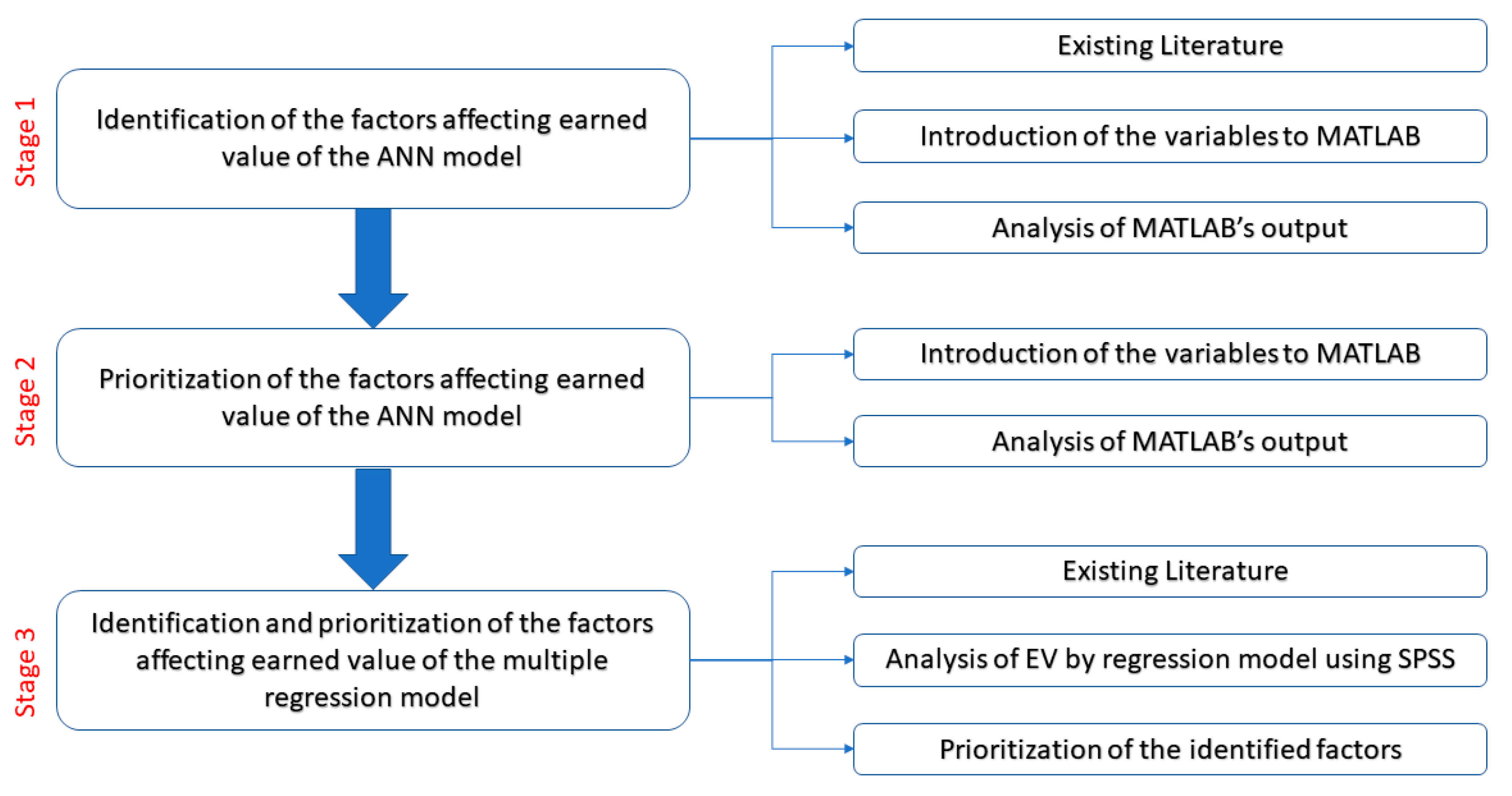
The methodology of the current study was determined according to the research aim. The main purpose of this research was to improve the prediction of the traditional EVM system in Fars road construction projects using an artificial neural network, as well as comparing it with a multiple regression model. The abovementioned main aim can be divided into three stages. Firstly, factors affecting the earned value of Fars road construction projects were determined using the existing literature. An artificial neural network was built in MATLAB, and the identified factors were introduced to the ANN model. In the next stage, the identified factors were prioritized in MATLAB using the ANN model. Finally, multiple regression was used as the analyzing tool, and the obtained results were compared with the ANN model. The abovementioned stages are summarized in Figure 1.

2.1. Predicting Earned Value Using Artificial Neural Network

Intelligent dynamic systems, such as ANNs, have been under researchers’ focus recently [44,45,46,47,48,49,50,51]. ANNs are able to identify the relationship among data by analyzing them and to then exploit this relationship in further analyses [52]. In fact, these computational intelligence-based systems attempt to model the neurosynaptic structure of the brain and are able to contribute to estimation, prediction and categorization problems effectively [53]. Generally, ANNs consist of three layers, namely, the input, hidden and output layers. Each of the abovementioned layers possesses its own neurons. It is important to mention that the number of hidden layers may be more than one according to the problem. In the current study, a multilayer perceptron network was used.

2.1.1. Input Data

Variables affecting the status of the project must be identified in order to investigate its future status. In fact, these variables are the input data of the artificial neural network. In this study, 14 factors affecting a project’s success were identified by investigating the existing literature, including books, journal papers and documents from the Fars State Road Administration. Due to the high sensitivity of this paper’s topic, the authors were not able to reduce the abovementioned number of factors. Some of the variables possessed numerical values, such as inflation rate. The inflation rate was derived from the Central Bank of Iran. However, there were variables that were not numerical, such as the qualification of the project management team. The abovementioned data were then quantified by scoring the variables from 1 to 5, where 1 and 5 stand for the worst and best status of a variable, respectively. In order to make it clearer, the qualitive status of a variable and its corresponding quantitative value are illustrated in

Table 1. Qualitive status of a variable and its corresponding value for analysis.

Qualitive Status	Quantitative Value
Critical	1
Very unsuitable	2
Unsuitable	3
Suitable	4
Very Suitable	5

. Ten questionnaires were filled out by experts for each project. Thus, 500 questionnaires were used for data gathering.

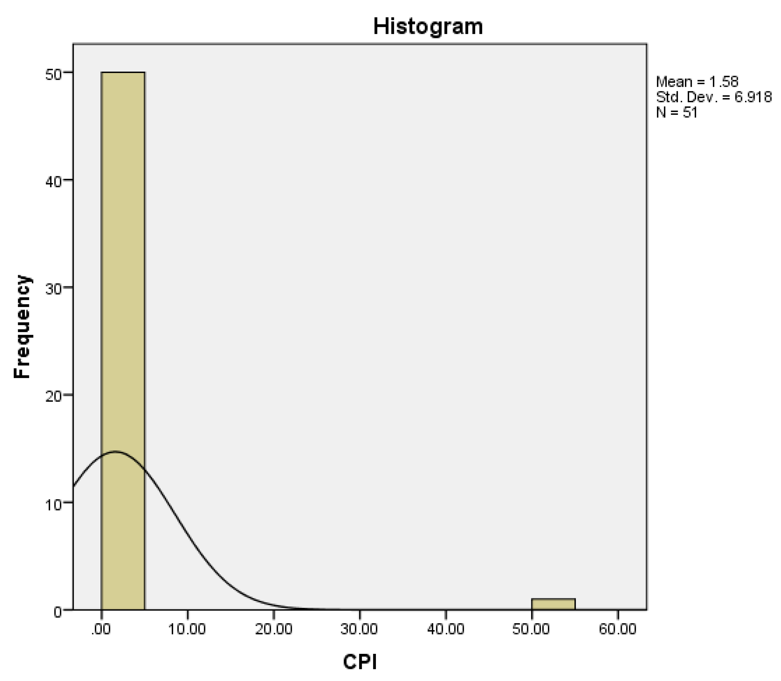
Using Microsoft Project files of the studied projects, the Cost Performance Index ($CPI$) of each project was extracted. Then, using Microsoft Excel, Mean Squared Error ($MSE$) was calculated. This error was used to compare the results of the ANN, multiple regression and the traditional EVM method. The BOX-COX method was used in order to normalize data using SPSS software. Then, the obtained data were exported to MATLAB software for further stages. $CPI$ and $MSE$ formulas are presented as follows [1,8,54,55]:

$$MSE=\frac{\sum \left(desiredoutput-predictedoutput\right)2}{noofdata}$$

(1)

$$CPI=\frac{BCWP}{ACWP}$$

(2)

where $BCWP$ and $ACWP$ stand for the actual cost of the work performed and the budgeted cost of the work performed, respectively.

2.1.2. Architecture of the Network

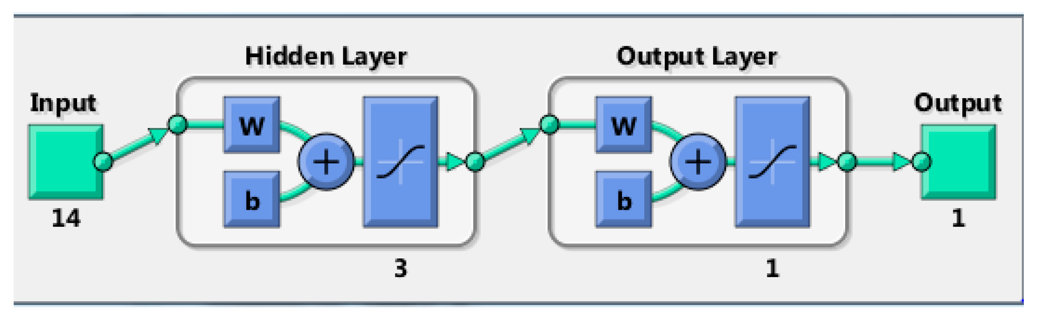
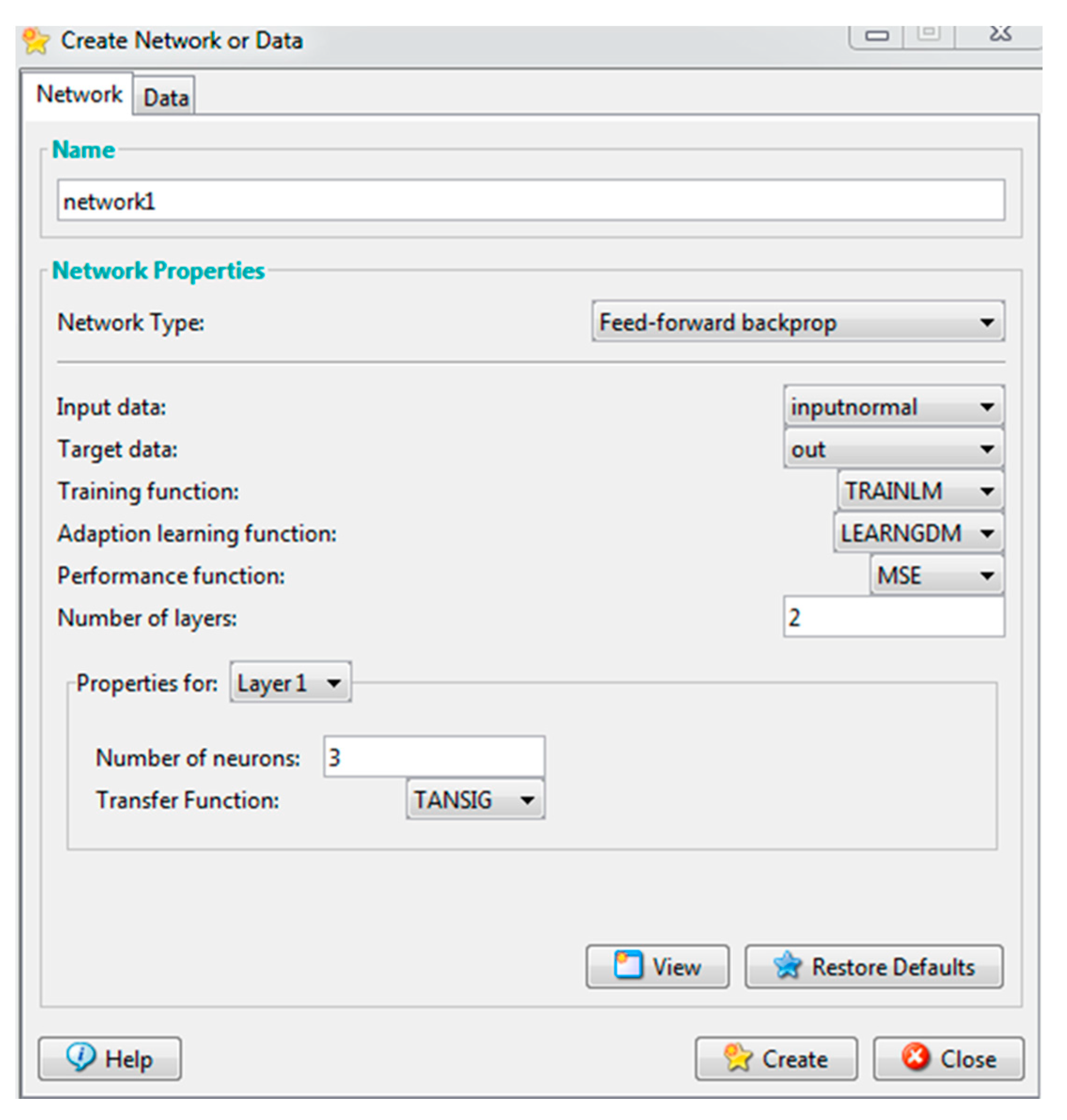
In this stage, the network’s architecture must be determined. In order to do so, the number of input, hidden and output layers should be specified [15]. In this study, an MLP (Multilayer perceptron) network is used in which the output of each layer is considered the input vector for the next layer. Each layer’s neurons have connections with the previous layer’s neurons. Each neuron’s duty is to calculate the net layer’s weight and pass data through a function called the transfer function. 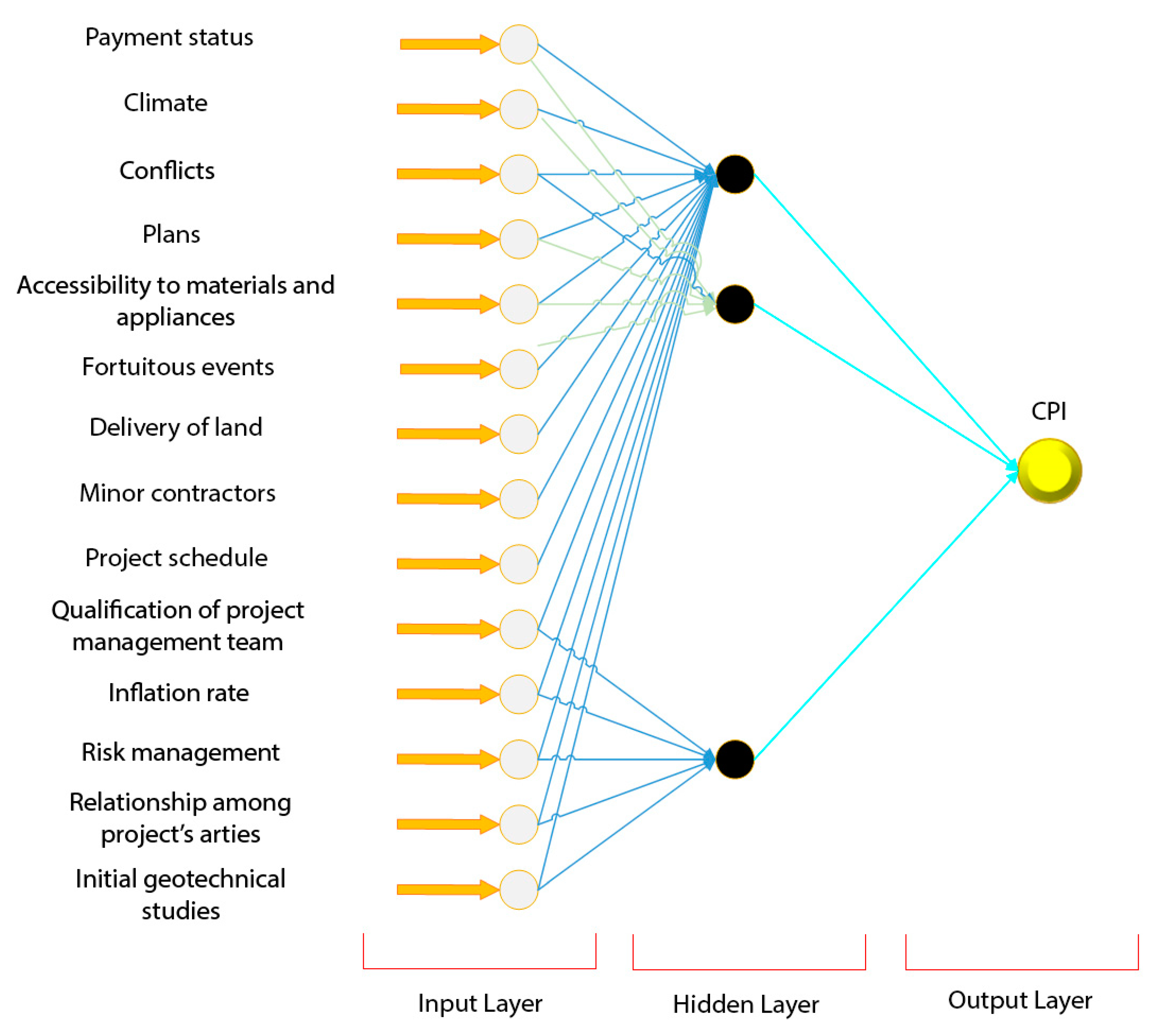Sigmoid Tangent is regarded as one of the most useful functions in this case and has been widely used by experts [56,57,58,59,60,61]. Thus, the abovementioned function was used as the transfer function. The final network in this research constitutes a multilayer perceptron neural network with 14 input variables in an input layer, a hidden layer and an output layer. The schematic structure of the designed neural network is illustrated in Figure 2.

2.2. Determination and Prioritization of Factors Using ANN

After training the network, output coefficients of introduced variables can be extracted from MATLAB software. As the artificial neural network considers all the introduced factors important, the prioritization of factors is conducted according to the coefficients.

2.3. Earned Value Prediction Using Multiple Regression Method

The correlation among dependent and independent variables can be determined using the multiple regression method [62]. There are four methods to enter input data into the model. These methods are the entering method (direct method), backward method, forward method and step-wise method [63]. In this study, the direct entering method was selected to be exploited. The linear relationship among the variables is illustrated below:

$$y_i=b_0+b_1{x}_{i1}+\cdots +b_p{x}_{ip}+e_i$$

(3)

where $p$ is the number of predictions, $b_{ j}$ is the value of the $j$th coefficient, $x_{ij}$ is the $i$th value of the $j$th prediction, and $e_i$ is the error of the $i$th value. Furthermore, the matrix form of the model is presented as follows:

$$Y=X\beta +\epsilon$$

(4)

where $\beta$ is the vector of regression coefficients, $\epsilon$ is the matrix of fitting errors, $Y$ is the vector of the dependent variable, and $X$ is the matrix of independent variables.

In order to determine and rank factors affecting the earned value of the studied projects, outputs of SPSS analyses were used. Variables with a significance of less than 0.05 were selected as effective factors. Furthermore, according to their significance value, variables were prioritized.

Finally, the ANN and the multiple regression model were compared according to the correlation coefficient and mean squared error of each model. The model possessing the higher correlation coefficient, as well as the lower MSE, was introduced as the preferable model [64].

2.4. Data Collection

In order to collect data, information regarding 50 road construction projects in Fars Province was extracted from documents. Then, besides other literature sources, data were turned into matrices and analyzed. As all factors affecting the cost of the abovementioned projects had to be considered, 14 factors were finally selected.

3. Results and Discussion

3.1. Predicting Earned Value Using Artificial Neural Network

3.1.1. Gathering the MLP Network’s Data

Data regarding road construction projects in Fars Province from 2010 to 2020 were gathered by conducting a vast study on documents from Fars Road Administration. Then, data were turned into matrices. In order to determine the best pattern of network input, all the probable factors affecting the cost of projects were determined. Thus, as input, 14 neurons were formed. These neurons were the identified factors, namely, “Payment status (F1)”, “Climate (F2)”, “Conflicts (F3)”, “Plans (F4)”, “Accessibility of materials and appliances (F5)”, “Fortuitous events (F6)”, “Delivery of land (F7)”, “Minor contractors (F8)”, “Project schedule (F9)”, “Qualification of project management team (F10)”, “Inflation rate (F11)”, “Risk management (F12)”, “Relationship among project’s parties (F13)” and “Initial geotechnical studies (F14)”. Moreover, the output layer of the ANN was determined, i.e., the cost performance index of the projects.

3.1.2. Normalizing Data

Using SPSS software, data were normalized in a range between −1 and 1. It seems necessary to mention that the ANN’s output can be returned to the initial format using the reverse algorithm. Normalized data are illustrated in

Table 2. Normalized ANN input data.

Project No.	F1	F2	F3	F4	F5	F6	F7	F8	F9	F10	F11	F12	F13	F14
1	0.70	0.90	0.50	0.50	0.63	0.63	0.63	0.70	0.50	0.70	0.21	0.70	0.70	0.70
2	0.30	0.90	0.10	0.70	0.90	0.63	0.37	0.50	0.90	0.90	0.61	0.30	0.90	0.70
3	0.70	0.63	0.10	0.70	0.63	0.90	0.10	0.90	0.90	0.70	0.31	0.70	0.70	0.90
4	0.30	0.10	0.30	0.50	0.37	0.37	0.63	0.50	0.70	0.30	0.49	0.50	0.50	0.90
5	0.10	0.37	0.70	0.10	0.10	0.63	0.37	0.90	0.90	0.70	0.31	0.70	0.70	0.70
6	0.10	0.10	0.70	0.50	0.37	0.63	0.37	0.90	0.30	0.50	0.49	0.50	0.30	0.90
7	0.70	0.63	0.30	0.70	0.37	0.37	0.63	0.30	0.10	0.30	0.39	0.10	0.50	0.30
8	0.70	0.37	0.90	0.30	0.90	0.10	0.90	0.10	0.10	0.70	0.39	0.30	0.70	0.30
9	0.50	0.10	0.10	0.50	0.37	0.90	0.63	0.30	0.70	0.70	0.90	0.50	0.90	0.70
10	0.50	0.37	0.70	0.10	0.37	0.63	0.10	0.50	0.10	0.70	0.39	0.70	0.30	0.70
11	0.10	0.37	0.10	0.90	0.90	0.37	0.63	0.50	0.90	0.90	0.49	0.70	0.50	0.70
12	0.50	0.10	0.30	0.70	0.10	0.37	0.10	0.30	0.90	0.70	0.31	0.30	0.50	0.50
13	0.10	0.90	0.10	0.70	0.63	0.63	0.63	0.50	0.30	0.70	0.31	0.90	0.10	0.50
14	0.70	0.63	0.70	0.90	0.10	0.37	0.63	0.10	0.50	0.90	0.49	0.30	0.30	0.90
15	0.50	0.37	0.70	0.30	0.37	0.90	0.37	0.70	0.50	0.50	0.49	0.90	0.10	0.10
16	0.70	0.10	0.50	0.90	0.90	0.37	0.37	0.90	0.90	0.50	0.49	0.30	0.70	0.70
17	0.50	0.37	0.50	0.90	0.63	0.90	0.10	0.50	0.10	0.50	0.77	0.30	0.10	0.10
18	0.90	0.90	0.50	0.30	0.10	0.63	0.90	0.90	0.70	0.90	0.49	0.50	0.70	0.30
19	0.30	0.37	0.50	0.70	0.63	0.63	0.90	0.90	0.50	0.50	0.77	0.30	0.50	0.10
20	0.90	0.37	0.70	0.30	0.37	0.90	0.37	0.50	0.70	0.30	0.19	0.70	0.30	0.90
21	0.70	0.90	0.50	0.90	0.63	0.63	0.90	0.70	0.30	0.30	0.31	0.10	0.10	0.70
22	0.70	0.37	0.70	0.50	0.63	0.63	0.90	0.10	0.50	0.70	0.12	0.90	0.70	0.30
23	0.90	0.90	0.50	0.50	0.63	0.37	0.90	0.90	0.50	0.90	0.39	0.70	0.50	0.50
24	0.90	0.37	0.70	0.70	0.63	0.63	0.63	0.70	0.90	0.90	0.39	0.90	0.50	0.50
25	0.90	0.37	0.50	0.30	0.90	0.90	0.37	0.70	0.70	0.30	0.49	0.50	0.70	0.30
26	0.90	0.90	0.50	0.90	0.63	0.63	0.90	0.90	0.30	0.70	0.19	0.50	0.50	0.50
27	0.10	0.10	0.50	0.70	0.63	0.63	0.37	0.30	0.50	0.70	0.49	0.70	0.90	0.50
28	0.10	0.63	0.50	0.70	0.10	0.63	0.37	0.90	0.70	0.10	0.10	0.30	0.50	0.50
29	0.50	0.63	0.90	0.30	0.90	0.90	0.90	0.50	0.30	0.50	0.10	0.50	0.70	0.10
30	0.10	0.37	0.30	0.50	0.37	0.63	0.37	0.10	0.50	0.50	0.49	0.30	0.90	0.30
31	0.50	0.10	0.70	0.70	0.63	0.37	0.90	0.70	0.30	0.30	0.61	0.30	0.10	0.90
32	0.50	0.37	0.30	0.30	0.37	0.90	0.90	0.50	0.70	0.30	0.49	0.10	0.30	0.50
33	0.10	0.63	0.50	0.70	0.10	0.90	0.10	0.90	0.90	0.30	0.16	0.50	0.30	0.10
34	0.50	0.37	0.50	0.50	0.90	0.63	0.63	0.70	0.30	0.90	0.49	0.30	0.90	0.50
35	0.90	0.10	0.10	0.50	0.63	0.37	0.63	0.70	0.70	0.70	0.12	0.90	0.50	0.70
36	0.30	0.37	0.70	0.70	0.37	0.90	0.63	0.30	0.70	0.50	0.49	0.50	0.50	0.10
37	0.10	0.63	0.10	0.50	0.90	0.37	0.37	0.70	0.30	0.50	0.90	0.90	0.90	0.30
38	0.30	0.90	0.30	0.90	0.63	0.63	0.63	0.50	0.70	0.70	0.39	0.70	0.90	0.10
39	0.30	0.90	0.50	0.50	0.37	0.90	0.63	0.90	0.30	0.50	0.31	0.10	0.10	0.30
40	0.70	0.10	0.50	0.10	0.90	0.90	0.37	0.90	0.90	0.70	0.49	0.90	0.50	0.30
41	0.70	0.63	0.30	0.50	0.37	0.63	0.90	0.50	0.70	0.30	0.78	0.30	0.70	0.50
42	0.30	0.90	0.50	0.30	0.10	0.63	0.10	0.50	0.30	0.30	0.78	0.50	0.10	0.30
43	0.70	0.10	0.10	0.30	0.37	0.90	0.63	0.10	0.70	0.30	0.49	0.70	0.70	0.90
44	0.50	0.37	0.90	0.70	0.63	0.90	0.37	0.50	0.30	0.30	0.39	0.10	0.50	0.50
45	0.30	0.37	0.10	0.30	0.37	0.63	0.63	0.90	0.50	0.70	0.10	0.70	0.50	0.90
46	0.90	0.63	0.70	0.10	0.37	0.37	0.63	0.90	0.70	0.50	0.39	0.50	0.30	0.10
47	0.30	0.37	0.10	0.50	0.37	0.90	0.63	0.50	0.70	0.10	0.21	0.30	0.70	0.50
48	0.10	0.37	0.30	0.50	0.63	0.37	0.37	0.30	0.90	0.90	0.49	0.30	0.90	0.30
49	0.90	0.37	0.30	0.70	0.37	0.90	0.37	0.50	0.70	0.90	0.31	0.30	0.90	0.50
50	0.10	0.63	0.10	0.30	0.90	0.63	0.90	0.30	0.50	0.70	0.90	0.70	0.50	0.10

.

3.1.3. Determining Hidden Layers of ANN

It is best for the number of hidden layers to be as low as possible. One hidden layer is initially considered for an ANN. Then, after training the ANN, the number of layers will be increased if the output is not suitable. Furthermore, there are a number of functions that can be used to produce the network’s outcome. In this study, the Sigmoid Tangent function was exploited. The network introduced into MATLAB software included 14 neurons in its input layer and 3 neurons in its hidden layer. The structure of the network is illustrated in Figure 3.

3.1.4. Training of the ANN

The introduced network in this study is an MLP network with back propagation error. The selected training function for the network was the Levenberg–Marquardt function due to its ability to converge fast. The transfer function was selected by trial and error, until the MSE reached the lowest value in both the training set and testing set. The data set was randomly divided into three groups. Seventy percent of the data was used for acquisition of the network, fifteen percent was used for testing the data, and fifteen percent was used for validation. The settings of the training ANN in MATLAB are demonstrated in Figure 4. The number of epochs was selected as 1000. As a result, the network reached its lowest acquisition error after 15 epochs. The network’s gradient function performance, MSE graph and regression graphs are shown in Figure 5, Figure 6 and Figure 7, respectively.

As a sample, one of the studied project’s Status Curve (S-Curve) was drawn using the trained ANN and was compared with the traditional EVM’s S-Curve. Improvement of the S-Curve is clearly seen in the figures below. Figure 8 and Figure 9 illustrate the traditional model and ANN’s S-Curves, respectively.

3.2. Determination and Prioritization of Factors Affecting Earned Value in the ANN

After training of the ANN in MATLAB, each variable is given a unique coefficient. Coefficients for the identified factors are illustrated in

Table 3. Prioritization and importance coefficients of the study factors using ANN.

Priority	Sign	Factor	Factor’s Coefficient
1	F1	Project Schedule	0.81
2	F2	Payment status	0.65
3	F3	Inflation rate	−0.58
4	F4	Fortuitous events	0.42
5	F5	Qualification of project management team	0.4
6	F6	Delivery of land	0.38
7	F7	Conflicts	−0.33
8	F8	Climate	0.24
9	F9	Minor contractors	0.21
10	F10	Plans	0.20
11	F11	Relationship among project’s parties	0.14
12	F12	Risk management	0.12
13	F13	Accessibility of materials and appliances	0.1
14	F14	Initial geotechnical studies	−0.017

.

According to the factors’ coefficients, the ANN’s function to predict the aim is obtained as follows:

$$\begin{array}{cc}n=\left(0.81\right)F1\hfill & \hfill +\left(0.65\right)F2-\left(0.58\right)F3+\left(0.42\right)F4+\left(0.4\right)F5+\left(0.38\right)F6-\left(0.33\right)F7\\ \hfill & +\left(0.24\right)F8+\left(0.21\right)F9+\left(0.2\right)F10+\left(0.14\right)F11+\left(0.12\right)F12\hfill \\ \hfill & +\left(0.1\right)F13-\left(0.017\right)F14\hfill \end{array}$$

(5)

Then, the final equation is obtained as follows:

$$CPI=tan\hspace{0.17em}sig\left(n\right)=\frac{2}{1+exp\left(-2n\right)}$$

(6)

3.3. Determination and Prioritization of Factors Affecting Earned Value Using Multiple Regression Method and Comparison with the ANN Model for Data Validation

3.3.1. Investigating the Condition of Using Multiple Regression Analysis

In this stage, SPSS software was exploited. The first condition if using linear regression is having normal data of earned value. Thus, a Kolmogorov–Smirnov test was conducted on the data in order to determine whether they were normal. The results illustrated that the data were not normal.

Table 4. Kolmogorov–Smirnov test for initial data.

Tests of Normality
	Kolmogorov–Smirnov
	Statistic	df	Sig.
CPI	0.519	51	0.000

and Figure 10 illustrate the information regarding the abovementioned test.

3.3.2. Analysis of Multiple Regression Model

Data analysis was conducted in order to validate the ANN results by comparing them with the multiple regression results. The correlation coefficient and determination coefficient of this study’s fitted multiple regression were 0.864 and 0.747, respectively. This means that about 74% of the dependent variable’s variance is determined according to the model’s independent variables. Information regarding the mentioned coefficients and the model analysis results is illustrated in

Table 5. Determination and correlation coefficients of the multiple regression model.

Model	R	R Square	Adjusted R Square
1	0.864	0.747	0.646

and

Table 6. Multiple regression model’s results.

Factor	Sign	Unstandardized Coefficients		Sig	Standardized Coefficients
		B	Std. Error		$\mathit{\beta }$
(Constant)		−4.999	1.154	0.000
Payment status	F2	0.155	0.065	0.022	0.230
Climate	F8	0.098	0.098	0.324	0.105
Conflicts	F7	0.201	0.084	0.023	0.254
Plans	F10	0.263	0.081	0.003	0.321
Accessibility of materials and appliances	F13	−0.031	0.105	0.766	−0.032
Fortuitous events	F4	−0.031	0.113	0.784	−0.026
Delivery of land	F6	0.062	0.096	0.523	0.062
Minor contractors	F9	0.208	0.072	0.007	0.283
Project schedule	F1	0.238	0.084	0.008	0.311
Qualification of project management team	F5	0.060	0.089	0.505	0.072
Inflation rate	F3	−0.029	0.014	0.040	−0.206
Risk management	F12	0.259	0.081	0.003	0.333
Relationship among project’s parties	F11	0.222	0.082	0.011	0.297
Initial geotechnical studies	F14	0.061	0.072	0.400	0.085

, respectively.

In Table 6, B and β stand for unstandardized coefficients and standardized coefficients, respectively. Although it is easier to write the multiple regression model’s equation using unstandardized coefficients, using standardized coefficients enables researchers to compare variables more easily. In other words, a higher value of the coefficient means that the variable can predict the outcome more effectively. According to the results, “Risk management”, “Plans”, “Project schedule”, “Relationship among project’s parties” and “Conflicts” are the most important factors.

In this study, an artificial neural network model for road construction projects was used in order to improve the prediction of the earned value. Moreover, a multiple regression model was used to validate the ANN results. The ANN and multiple regression models’ calculated mean squared errors and the real values of projects are illustrated in

Table 7. Comparison of the ANN and multiple regression models.

MSE	R	Model
0.0152	0.727	Traditional EVM
0.00206	0.896	ANN
0.012	0.864	Multiple regression

. As it is easily seen, both the ANN model and the multiple regression model possess low errors. Moreover, the ANN model not only had the lowest error, but also possessed the most effective prediction coefficient.

4. Conclusions

Perceptron neural networks, especially multilayer perceptron networks, are considered to be some of the best neural networks. In this study, it was observed that these networks were able to perform a non-linear mapping with desirable accuracy by selecting a suitable number of layers and neurons. As these neural networks possess the two main features of experimental data-based learning and parallel generalization ability, they are highly suitable for sophisticated systems that are impossible or difficult to model. Artificial neural networks are more accurate in comparison to other methods due to their usage of proven mathematical formulas possessing the lowest possible errors. One of the aspects that limit the usage of artificial neural networks is the difficulty faced when training them. These networks produce better results when they receive a large group of data. However, adjusting the parameters of network training is a difficult task that requires experience and a lot of trial and error. Furthermore, convergence to an incorrect answer, keeping internal information instead of learning it, and requiring a lot of time for training are other difficulties associated with using artificial neural networks.

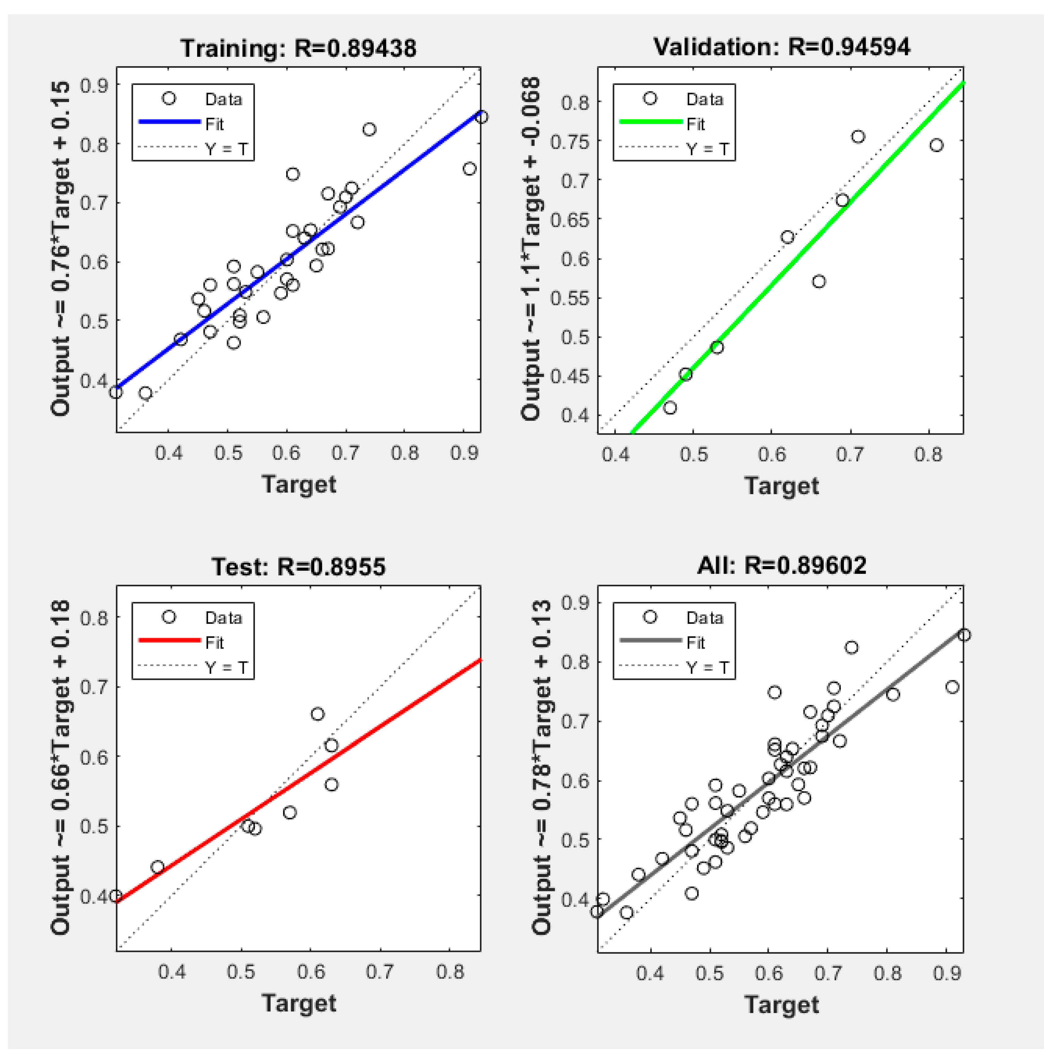
In this research, two different models, i.e., an artificial neural network model and a multiple regression model, were designed and analyzed in order to improve the traditional earned value management system. The latter model was used as a validation test for the ANN model. Road construction projects in Fars Province, Iran, between 2010 and 2020 were investigated as a case study. Fourteen factors affecting the earned value of these projects were identified. According to the ANN results, “Project plan”, “Payment status”, “Inflation rate”, “Fortuitous events” and “Qualification of project management team” with coefficients of 0.81, 0.65, −0.58, 0.42 and 0.4 were the top five influencing factors, respectively. On the other hand, according to the multiple regression model results, “Risk management”, “Plans”, “Project schedule”, “Relationship among project’s parties” and “Conflicts” with standardized coefficients of 0.333, 0.321, 0.311, 0.297 and 0.254, respectively, were the most important factors. A comparison of the two models illustrated that both models result in better results in comparison to the traditional EVM method. Moreover, the ANN model with an MSE of 0.00206 and an R value of 0.896 was selected as the best model.

The methods used in this study could also be used to tackle other problems in the construction industry. The results obtained in this study will help road construction industry members to predict the earned value of future projects more precisely. ANN models are highly recommended by the authors for use in other construction problems. Furthermore, it is suggested that prospective researchers focus on more complex construction projects in order to investigate the performance criteria more deeply [65].

References

1. Mahalakshmi, G.; Rajasekaran, C. Early cost estimation of highway projects in India using artificial neural network. In Sustainable Construction and Building Materials Lecture Notes in Civil Engineering; Das, B., Neithalath, N., Eds.; Springer: Singapore, 2019; Volume 25, pp. 659–672. [Google Scholar]
2. Wideman, R.M. Cost Control of Capital Projects and the Project Cost Management System Requirements: A Handbook for Owners, Architects, Engineers, and All Those Involved in Project Management of Constructed Facilities; AEW Services, BiTech Publishers: Richmond, BC, Canada, 1995. [Google Scholar]
3. Al-Zwainy, F.M.; Aidan, I.A.-A. Forecasting the cost of structure of infrastructure projects utilizing artificial neural network model (highway projects as case study). Indian J. Sci. Technol. 2017, 10, 1–12. [Google Scholar] [CrossRef] [Green Version]
4. Turochy, R.E.; Hoel, L.A.; Doty, R.S. Highway Project Cost Estimating Methods Used in the Planning Stage of Project Development; Virginia Transportation Research Council: Charlottesville, VA, USA, 2001. [Google Scholar]
5. Sodikov, J. Cost estimation of highway projects in developing countries: Artificial neural network approach. J. East. Asia Soc. Transp. Stud. 2005, 6, 1036–1047. [Google Scholar]
6. Czernigowska, A. Earned value method as a tool for project control. Bud. Archit. 2008, 3, 15–32. [Google Scholar]
7. Anbari, F.T. Earned value project management method and extensions. Proj. Manag. J. 2003, 34, 12–23. [Google Scholar] [CrossRef]
8. Koke, B.; Moehler, R.C. Earned Green Value Management for Project Management: A systematic review. J. Clean. Prod. 2019, 230, 180–197. [Google Scholar] [CrossRef]
9. Bryde, D.; Unterhitzenberger, C.; Joby, R. Conditions of success for earned value analysis in projects. Int. J. Proj. Manag. 2018, 36, 474–484. [Google Scholar] [CrossRef]
10. Colin, J.; Vanhoucke, M. A comparison of the performance of various project control methods using earned value management systems. Expert Syst. Appl. 2015, 42, 3159–3175. [Google Scholar] [CrossRef]
11. Kerkhove, L.-P.; Vanhoucke, M. Extensions of earned value management: Using the earned incentive metric to improve signal quality. Int. J. Proj. Manag. 2017, 35, 148–168. [Google Scholar] [CrossRef]
12. Abdi, A.; Taghipour, S.; Khamooshi, H. A model to control environmental performance of project execution process based on greenhouse gas emissions using earned value management. Int. J. Proj. Manag. 2018, 36, 397–413. [Google Scholar] [CrossRef]
13. Sutrisna, M.; Pellicer, E.; Torres-Machi, C.; Picornell, M. Exploring earned value management in the Spanish construction industry as a pathway to competitive advantage. Int. J. Constr. Manag. 2020, 20, 1–12. [Google Scholar] [CrossRef]
14. De Andrade, P.A.; Martens, A.; Vanhoucke, M. Using real project schedule data to compare earned schedule and earned duration management project time forecasting capabilities. Autom. Constr. 2019, 99, 68–78. [Google Scholar] [CrossRef]
15. Kulkarni, P.; Londhe, S.; Deo, M. Artificial neural networks for construction management: A review. J. Soft Comput. Civ. Eng. 2017, 1, 70–88. [Google Scholar]
16. Adeli, H.; Yeh, C. Perceptron learning in engineering design. Comput. Aided Civ. Infrastruct. Eng. 1989, 4, 247–256. [Google Scholar] [CrossRef]
17. Adeli, H. Neural networks in civil engineering: 1989–2000. Comput. Aided Civ. Infrastruct. Eng. 2001, 16, 126–142. [Google Scholar] [CrossRef]
18. Peško, I.; Mučenski, V.; Šešlija, M.; Radović, N.; Vujkov, A.; Bibić, D.; Krklješ, M. Estimation of costs and durations of construction of urban roads using ANN and SVM. Complexity 2017, 2017, 2450370. [Google Scholar] [CrossRef] [Green Version]
19. Albino, V.; Garavelli, A.C. A neural network application to subcontractor rating in construction firms. Int. J. Proj. Manag. 1998, 16, 9–14. [Google Scholar] [CrossRef]
20. Leung, A.W.; Tam, C.; Liu, D. Comparative study of artificial neural networks and multiple regression analysis for predicting hoisting times of tower cranes. Build. Environ. 2001, 36, 457–467. [Google Scholar] [CrossRef]
21. Cheung, S.O.; Wong, P.S.P.; Fung, A.S.; Coffey, W. Predicting project performance through neural networks. Int. J. Proj. Manag. 2006, 24, 207–215. [Google Scholar] [CrossRef] [Green Version]
22. Vouk, D.; Malus, D.; Halkijevic, I. Neural networks in economic analyses of wastewater systems. Expert Syst. Appl. 2011, 38, 10031–10035. [Google Scholar] [CrossRef]
23. Mučenski, V.; Trivunić, M.; Ćirović, G.; Peško, I.; Dražić, J. Estimation of recycling capacity of multi-storey building structures using artificial neural networks. Acta Polytech. Hung. 2013, 10, 175–192. [Google Scholar]
24. Chaphalkar, N.; Iyer, K.; Patil, S.K. Prediction of outcome of construction dispute claims using multilayer perceptron neural network model. Int. J. Proj. Manag. 2015, 33, 1827–1835. [Google Scholar] [CrossRef]
25. Golnaraghi, S.; Zangenehmadar, Z.; Moselhi, O.; Alkass, S. Application of artificial neural network (s) in predicting formwork labour productivity. Adv. Civ. Eng. 2019, 2019, 5972620. [Google Scholar] [CrossRef] [Green Version]
26. Tijanić, K.; Car-Pušić, D.; Šperac, M. Cost estimation in road construction using artificial neural network. Neural Comput. Appl. 2020, 32, 9343–9355. [Google Scholar] [CrossRef]
27. Casilari-Perez, E.; García-Lagos, F. A comprehensive study on the use of artificial neural networks in wearable fall detection systems. Expert Syst. Appl. 2019, 138, 112811. [Google Scholar] [CrossRef]
28. Kim, H.-J.; Jo, N.-O.; Shin, K.-S. Optimization of cluster-based evolutionary undersampling for the artificial neural networks in corporate bankruptcy prediction. Expert Syst. Appl. 2016, 59, 226–234. [Google Scholar] [CrossRef]
29. Kocadagli, O.; Langari, R. Classification of EEG signals for epileptic seizures using hybrid artificial neural networks based wavelet transforms and fuzzy relations. Expert Syst. Appl. 2017, 88, 419–434. [Google Scholar] [CrossRef]
30. Kwon, H.-B.; Lee, J.; Davis, K.N.W. Neural network modeling for a two-stage production process with versatile variables: Predictive analysis for above-average performance. Expert Syst. Appl. 2018, 100, 120–130. [Google Scholar] [CrossRef]
31. Bandara, K.; Bergmeir, C.; Smyl, S. Forecasting across time series databases using recurrent neural networks on groups of similar series: A clustering approach. Expert Syst. Appl. 2020, 140, 112896. [Google Scholar] [CrossRef] [Green Version]
32. Yazdani-Chamzini, A.; Zavadskas, E.K.; Antucheviciene, J.; Bausys, R. A model for shovel capital cost estimation, using a hybrid model of multivariate regression and neural networks. Symmetry 2017, 9, 298. [Google Scholar] [CrossRef] [Green Version]
33. Juszczyk, M.; Leśniak, A. Modelling construction site cost index based on neural network ensembles. Symmetry 2019, 11, 411. [Google Scholar] [CrossRef] [Green Version]
34. AlHares, E.F.T.; Budayan, C. Estimation at completion simulation using the potential of soft computing models: Case study of construction engineering projects. Symmetry 2019, 11, 190. [Google Scholar] [CrossRef] [Green Version]
35. Juszczyk, M.; Zima, K.; Lelek, W. Forecasting of sports fields construction costs aided by ensembles of neural networks. J. Civ. Eng. Manag. 2019, 25, 715–729. [Google Scholar] [CrossRef] [Green Version]
36. Shan, M.; Le, Y.; Yiu, K.T.; Chan, A.P.; Hu, Y.; Zhou, Y. Assessing collusion risks in managing construction projects using artificial neural network. Technol. Econ. Dev. Econ. 2018, 24, 2003–2025. [Google Scholar] [CrossRef]
37. Tadewos, S.G.; Patel, D. Factors influencing time and cost overruns in road construction projects: Addis Ababa, Ethiopian scenario. Int. Res. J. Eng. Technol. 2018, 5, 177–180. [Google Scholar]
38. Ökmen, Ö.; Öztaş, A. Construction cost analysis under uncertainty with correlated cost risk analysis model. Constr. Manag. Econ. 2010, 28, 203–212. [Google Scholar] [CrossRef]
39. Plebankiewicz, E. Model of predicting cost overrun in construction projects. Sustainability 2018, 10, 4387. [Google Scholar] [CrossRef] [Green Version]
40. Habibi, M.; Kermanshachi, S.; Safapour, E. Engineering, procurement and construction cost and schedule performance leading indicators: State-of-the-art review. In Proceedings of the Construction Research Congres, New Orleans, LA, USA, 2–4 April 2018; pp. 2–4. [Google Scholar]
41. Flyvbjerg, B.; Holm, M.S.; Buhl, S. Cost Underestimation in Public Works Projects: Error or Lie? Aalborg University, Department of Development and Planning: Aalborg, Denmark, 2004. [Google Scholar]
42. Heravi, G.; Mohammadian, M. Investigating cost overruns and delay in urban construction projects in Iran. Int. J. Constr. Manag. 2019, 1–11. [Google Scholar] [CrossRef]
43. Moura, H.M.P.; Teixeira, J.M.C.; Pires, B. Dealing with cost and time in the Portuguese construction industry. In Proceedings of the CIB World Building Congress, Cape Town, South Africa, 14–17 May 2007; pp. 1252–1265. [Google Scholar]
44. Bai, S.; Fang, G.; Zhou, J. Construction of three-dimensional extrusion limit diagram for magnesium alloy using artificial neural network and its validation. J. Mater. Process Technol. 2020, 275, 116361. [Google Scholar] [CrossRef]
45. Nov, P.; Peansupap, V. Using artificial neural network for selecting type of subcontractor relationships in construction project. Eng. J. 2020, 24, 73–88. [Google Scholar] [CrossRef]
46. Jang, H.-S.; Shuli, X.; So, S.-Y. Analysis the compressive strength of flue gas desulfurization gypsum using artificial neural network. J. Nanosci. Nanotechnol. 2020, 20, 485–490. [Google Scholar] [CrossRef] [PubMed]
47. Ghanizadeh, A.R.; Abbaslou, H.; Amlashi, A.T.; Alidoust, P. Modeling of bentonite/sepiolite plastic concrete compressive strength using artificial neural network and support vector machine. Front. Struct. Civ. Eng. 2019, 13, 215–239. [Google Scholar] [CrossRef]
48. Chesnokov, A.; Mikhailov, V.; Dolmatov, I. Evaluation of adverse factors acting on a pre-stressed wire rope structure by means of artificial neural network. In Proceedings of the 1st International Conference on Control Systems, Mathematical Modelling, Automation and Energy Efficiency (SUMMA), Lipetsk, Russia, 20–22 November 2019; pp. 500–504. [Google Scholar]
49. Hammoudi, A.; Moussaceb, K.; Belebchouche, C.; Dahmoune, F. Comparison of artificial neural network (ANN) and response surface methodology (RSM) prediction in compressive strength of recycled concrete aggregates. Constr. Build. Mater. 2019, 209, 425–436. [Google Scholar] [CrossRef]
50. Roh, Y.; Choi, E.; Choi, Y. An artificial neural network based phrase network construction method for structuring facility error types. J. Internet Comput. Serv. 2018, 19, 21–29. [Google Scholar]
51. Johnson, J.; Hossain-McKenzie, S.; Bui, U.; Etigowni, S.; Davis, K.; Zonouz, S. Improving power system neural network construction using modal analysis. In Proceedings of the 19th International Conference on Intelligent System Application to Power Systems (ISAP), San Antonio, TX, USA, 17–20 September 2017; pp. 1–6. [Google Scholar]
52. Veelenturf, L.P. Analysis and Applications of Artificial Neural Networks; Prentice-Hall, Inc.: Upper Saddle River, NJ, USA, 1995. [Google Scholar]
53. Beale, M.H.; Hagan, M.T.; Demuth, H.B. Neural Network Toolbox; User’s Guide MathWorks: Natick, MA, USA, 2010; Volume 2, pp. 77–81. [Google Scholar]
54. McRoberts, R.E.; Næsset, E.; Gobakken, T.; Chirici, G.; Condés, S.; Hou, Z.; Saarela, S.; Chen, Q.; Ståhl, G.; Walters, B.F. Assessing components of the model-based mean square error estimator for remote sensing assisted forest applications. Can. J. For. Res. 2018, 48, 642–649. [Google Scholar] [CrossRef]
55. Vanhoucke, M. Measuring Time: Improving Project Performance Using Earned Value Management; Springer Science & Business Media: Berlin/Heidelberg, Germany, 2009; Volume 136. [Google Scholar]
56. Zadeh, M.R.; Amin, S.; Khalili, D.; Singh, V.P. Daily outflow prediction by multi layer perceptron with logistic sigmoid and tangent sigmoid activation functions. Water Resour. Manag. 2010, 24, 2673–2688. [Google Scholar] [CrossRef]
57. Datta, D.; Agarwal, S.; Kumar, V.; Raj, M.; Ray, B.; Banerjee, A. Design of current mode sigmoid function and hyperbolic tangent function. In Proceedings of the International Symposium on VLSI Design and Test, Sapporo, Japan, 26–29 May 2019; pp. 47–60. [Google Scholar]
58. Namin, A.H.; Leboeuf, K.; Muscedere, R.; Wu, H.; Ahmadi, M. Efficient hardware implementation of the hyperbolic tangent sigmoid function. In Proceedings of the IEEE International Symposium on Circuits and Systems, Taipei, Taiwan, 24–27 May 2009; pp. 2117–2120. [Google Scholar]
59. Leboeuf, K.; Namin, A.H.; Muscedere, R.; Wu, H.; Ahmadi, M. High speed VLSI implementation of the hyperbolic tangent sigmoid function. In Proceedings of the Third International Conference on Convergence and Hybrid Information Technology, Busan, Korea, 11–13 November 2008; pp. 1070–1073. [Google Scholar]
60. Lin, C.-W.; Wang, J.-S. A digital circuit design of hyperbolic tangent sigmoid function for neural networks. In Proceedings of the IEEE International Symposium on Circuits and Systems, Seattle, WA, USA, 18–21 May 2008; pp. 856–859. [Google Scholar]
61. Koyuncu, I. Implementation of high speed tangent sigmoid transfer function approximations for artificial neural network applications on FPGA. Adv. Electr. Comput. Eng. 2018, 18, 79–86. [Google Scholar] [CrossRef]
62. Asiltürk, I.; Çunkaş, M. Modeling and prediction of surface roughness in turning operations using artificial neural network and multiple regression method. Expert Syst. Appl. 2011, 38, 5826–5832. [Google Scholar] [CrossRef]
63. Gao, Y.; Cowling, M. Introduction to Panel Data, Multiple Regression Method, and Principal Components Analysis Using Stata: Study on the Determinants of Executive Compensation—A Behavioral Approach Using Evidence from Chinese Listed Firms; SAGE Publications: Thousand Oaks, CA, USA, 2019. [Google Scholar]
64. Yilmaz, I.; Kaynar, O. Multiple regression, ANN (RBF, MLP) and ANFIS models for prediction of swell potential of clayey soils. Expert Syst. Appl. 2011, 38, 5958–5966. [Google Scholar] [CrossRef]
65. Stumpe, F.; Katina, P.F. Multi-objective multi-customer project network: Visualising interdependencies and influences. Int. J. Syst. Syst. Eng. 2019, 9, 139–166. [Google Scholar] [CrossRef]
Figure 1. Research methodology according to the study aim.
Symmetry 12 01745 g001
Figure 2. Schematic structure of the Artificial Neural Network (ANN).
Symmetry 12 01745 g002
Figure 3. ANN introduced into MATLAB.
Symmetry 12 01745 g003
Figure 4. Settings of the training ANN in MATLAB.
Symmetry 12 01745 g004
Figure 5. ANN’s gradient function performance.
Symmetry 12 01745 g005
Figure 6. Mean Squared Error (MSE) graph of the trained ANN.
Symmetry 12 01745 g006
Figure 7. ANN’s regression graphs.
Symmetry 12 01745 g007
Figure 8. Sample project’s S-Curve according to the traditional Earned Value Management (EVM) model.
Symmetry 12 01745 g008
Figure 9. Sample project’s S-Curve according to the ANN model.
Symmetry 12 01745 g009
Figure 10. Normalization test histogram.
Symmetry 12 01745 g010