Diffusion-Limited Reaction Kinetics of a Reactant with Square Reactive Patches on a Plane

Department of Chemistry, Hankuk University of Foreign Studies, Yongin 17035, Korea
Symmetry 2020, 12(10), 1744; https://doi.org/10.3390/sym12101744
Submission received: 23 September 2020
/
Revised: 19 October 2020
/
Accepted: 20 October 2020
/
Published: 21 October 2020
(This article belongs to the Special Issue Advances in Theoretical and Computational Chemistry)
Abstract
:We present a simple reaction model to study the influence of the size, number, and spatial arrangement of reactive patches on a reactant placed on a plane. Specifically, we consider a reactant whose surface has an N × N square grid structure, with each square cell (or patch) being chemically reactive or inert for partner reactant molecules approaching the cell via diffusion. We calculate the rate constant for various cases with different reactive N × N square patterns using the finite element method. For N = 2, 3, we determine the reaction kinetics of all possible reactive patterns in the absence and presence of periodic boundary conditions, and from the analysis, we find that the dependences of the kinetics on the size, number, and spatial arrangement are similar to those observed in reactive patches on a sphere. Furthermore, using square reactant models, we present a method to significantly increase the rate constant by sequentially breaking the patches into smaller patches and arranging them symmetrically. Interestingly, we find that a reactant with a symmetric patch distribution has a power–law relation between the rate constant and the number of reactive patches and show that this works well when the total reactive area is much less than the total surface area of the reactant. Since our N × N discrete models enable us to examine all possible reactive cases completely, they provide a solid understanding of the surface reaction kinetics, which would be helpful for understanding the fundamental aspects of the competitions between reactive patches arising in real applications.

1. Introduction
In a reaction between A and B, two reactant A molecules can compete with each other for a partner reactant B molecule, the outcome of which is strongly dependent on how close the competing A molecules are to each other [1,2]. A similar competition also occurs between two reactive sites on a reactant surface [3,4,5] and can be generalized to cases of multiple sites [6,7]. One specific example of the latter is a cell surface with multiple receptors competing for ligands [8]. This case has been intensively studied through a simple model, in which the cell surface is modeled as a sphere with multiple circular patches [8,9,10,11,12,13,14,15,16,17,18,19,20,21], using analytical theories, such as the effective medium treatment [11], the homogenization theory [9,12,14,15], the matched asymptotic analysis [16], and the curvature-dependent kinetic theory [19], and numerical methods, such as Brownian dynamics simulations [10,12,13,17], the spectral boundary element method [18], and the finite element method [7]. Moreover, recently, other related models have been proposed and studied using the matched asymptotic analysis [22,23]. Despite these advances in the study of multiple reactive patches on a sphere, the study of the effect of the spatial patch arrangement on kinetics is mostly limited to a random, symmetric, or certain type of arrangement of patches [7]. A study involving the complete examination of all possible arrangements has not been performed.
In a reactant with multiple reactive sites, any two reactive sites can kinetically compete with each other, depending on their distance, and, therefore, their overall arrangement on the surface can significantly affect the overall reaction kinetics [7]. However, for continuum models such as reactive sites on infinite planes, since the sites can be placed at any location as long as the sites do not overlap, an infinite number of site arrangements exist, which increases the difficulty in investigating all possible arrangements. Even for a spherical reactant with a finite surface area, because of the space continuum, an infinite number of arrangements of reactive sites (patches) also exist, except for the cases in which the sites are maximally occupied on the surface such that no room exists for one to rearrange the sites, meaning that only one arrangement is available. Therefore, in this work, we focus on the development of a model that can generate a finite number of site arrangements, and we study the kinetics of that model.
To generate a finite number of arrangements, we consider the discretization of the surface of the reactant. One intuitive way to accomplish this is to create an N × N grid on the surface, with each cell defined by the grid lines, being either reactive or inert. When a cell is reactive, we can consider it a reactive patch. Furthermore, for our convenience, we assume that the shape of the reactant is a square, and consequently, a square with N × N grid generates N × N cells. Depending on which cell is reactive, the model can generate a variety of reactants; for example, when all cells are reactive, the reactant is fully reactive. We also assume that the reactant is on a plane, such that the N × N cells are identical in shape. If the reactant is on a curved surface, the surface curvature must be considered, and the N × N cells will have different shapes. Because of the N × N square shape of the reactant, we call this model the N × N square reactant model. Another discrete model based on a triangular lattice or square lattice has been proposed, but that model study was focused on clusters of reactive N-disk patches [24]; in our model, we consider the cases of both separate patches on a reactant and clustered ones.
In this work, we first study the simplest cases of N = 2, 3 to see how the square reactant model works. As we did previously for a spherical reactant with multiple reactive patches [7], we study how the unit cell size, number, and arrangement of reactive patches affect the reaction kinetics. However, the variation in patch arrangement for N = 2, 3 is limited because of the small number of cells on the surface (4 and 9 cells for N = 2 and 3, respectively). To overcome this limitation and to obtain a general idea regarding the effect of the patch arrangements, we also study the extended model of N = 9 with some representative arrangements of reactive cells. Based on this understanding, we discuss how one can increase the overall rate constant for a given total reactive patch area. For the discussion, we propose a systematic way of increasing the rate constant by properly arranging reactive cells in a symmetric way.
This paper is organized as follows. In Section 2, we explain in detail our N × N square reactant models and computational methodologies. In Section 3, we perform a complete kinetic study of the 2 × 2 and 3 × 3 square models for two types of models (one with normal boundary conditions and one with periodic boundary conditions) and discuss the significance of the results. Using the square models, we also investigate the dependence of kinetics on the fraction of the total reactive patch area and the effect of the patch distribution. Based on these investigations, we propose a systematic way to increase the rate constant by breaking and symmetrically arranging reactive patches for a fixed surface coverage ratio of reactive patches. Furthermore, we discuss a very interesting power–law relationship between the rate constant and the number of patches. In Section 4, we conclude by summarizing our findings from this work.
2. Reaction Models and Computational Methods
2.1. Reaction Models
In this investigation, we use two types of reaction models to study a diffusion-limited (or diffusion-controlled) bimolecular reaction between reactants A and B. Here, reactant A is the one we are most interested in because it is a square reactant with a reactive patch distribution, while reactant B is simply a point-like particle. One type is for the situation where reactant A is localized on a certain chemically-inert plane. The other type is for the situation where reactant A has a large surface area or is enlarged for detained analysis; thus, its reactive patches are assumed to exist on the entire surface of the model.
The first type of model was used in our previous study [7,25]. A schematic diagram of the reaction model is shown in Figure 1. Reactant A is placed at the origin of the coordinate system and is on a nonreactive x-y plane at z = 0. The surface of reactant A has a square grid with N × N cells, where N is the number of cells on each side. Each cell is reactive or inert for the reaction with the reactant B; when the cell is reactive, it is considered a reactive patch. Around reactant A (black square lines on the x-y plane in Figure 1), we assume that many point-like molecules of reactant B exist that do not interact with each other and freely move with a diffusion coefficient . When a molecule of reactant B contacts one of the reactive patches of reactant A, the reaction occurs immediately. Specifically, the reaction rate is solely determined by the transport rate at which B molecules diffuse to the reactive patches of A; this is why we called this reaction a diffusion-limited (or diffusion-controlled) reaction. The reaction process above can be described by the Smoluchowski equation for the concentration of reactant B, which is basically a diffusion equation with boundary conditions describing reactions. Here, to further simplify, we normalize the concentration of reactant B by the bulk-solution concentration of B, which is the concentration far away from A, such that the concentration of B or is a dimensionless variable. We also assume that our model system is in a steady state. Consequently, the Smoluchowski equation governing the reaction kinetics is described by a time-independent diffusion equation as follows:
where is the diffusion coefficient of reactant B and is the concentration of reactant B at the position .
To solve Equation (1), we set up the boundary conditions as follows: (a) on the reactive patches of A, is zero (absorbing boundary condition), or , where refers to the reactive patches; (b) on the remaining non-reactive surface area of A, the flux of B onto A is zero (reflecting boundary condition), or , where is the normal vector from the reactant surface at ; (c) on the area of the x-y plane outside reactant A, the flux of B onto the area is also zero (reflecting boundary condition), or ; (d) at locations far from A, is 1 (bulk-solution concentration), meaning that no reactions occur when B is far from A. For boundary (d), we can define an outer boundary; for example, in Figure 1, the blue hemisphere of radius represents an outer boundary condition, which is . Therefore, we solve the Smoluchowski equation for a bounded domain confined by the x-y plane containing reactant A at z = 0 and a hemisphere of radius with z > 0 (see the inner space created by the blue lines in Figure 1). In this work, we set a dimensionless value of to 10, as was used in our previous work [25], while a dimensionless length of each side of square reactant A is 1.8.
By solving Equation (1), we obtain , and from , we calculate the rate constant by calculating the fluxes of B at the reactive patches of A, which is given by
where is the surface area element of patch .
Per usual [7], we finally calculate the rate constant normalized by the rate constant for the case in which the entire reactant surface is reactive. Specifically, this normalized rate constant is simply calculated by and was denoted by . Here, we note that the maximum value of is 1.
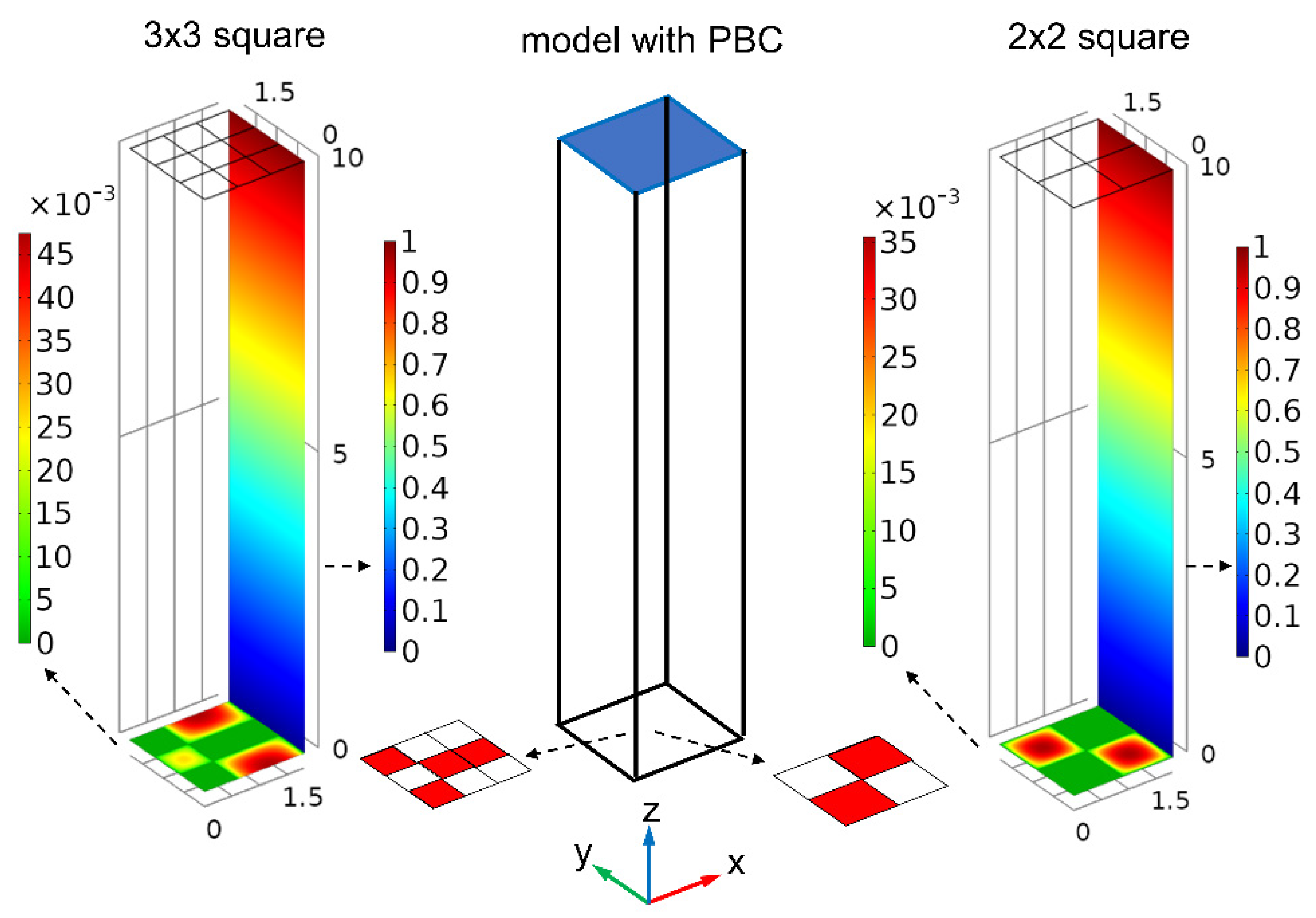
In the first type of model, reactant A is localized on a plane, and the reactant has a finite surface area. However, when reactant A has a very large surface area or when a particular reactant area of interest is enlarged, we need to consider only the reactant surface without other parts of the x-y plane; thus, we may assume on that length scale that the reactant surface is an infinite surface. In this case, we can consider the second type of model. In the second type, we remove the 4th boundary condition (d) and instead introduce the new boundary condition (d)’, i.e., periodic boundary conditions (PBCs) for the x and y coordinates, which are typically used for molecular dynamic simulations [26], and an outer boundary condition for the z coordinate, which is . Because of the PBCs, a reactive patch structure is periodically repeated in the x and y dimensions. From the boundary condition (d)’, we, therefore, need to solve the Smoluchowski equation for a bounded domain along the z-axis from the reactant surface at z = 0 to the outer boundary at z =, with the periodicity along the x- and y-axes (see the inner space of the rectangular prism at the center in Figure 2). In this work, we set a dimensionless value of to 10, while a dimensionless length of each side of the square reactant is 1.8.
Figure 2 shows a schematic diagram of this second type of model. As with the first type of model, we solve the Smoluchowski equation or Equation (1) to obtain and calculate the rate constant by Equation (2) and eventually calculate the normalized rate constant or ., where is the rate constant when the reactant surface is fully reactive.
2.2. Computational Methods
To solve the Smoluchowski equations for our models with N × N square reactants, we use the finite element method (FEM), a popular numerical method for solving partial differential equations with complicated boundary conditions. Specifically, for the FEM calculations, we use the software COMSOL [COMSOL Multiphysics® v.5.4, COMSOL AB, Stockholm, Sweden], an FEM software package. In our models, to achieve high accuracy in the FEM calculations, we use very fine meshes in the regions of and near the reactive patches; in the mesh construction, the mesh for the region of the reactive patches is “extremely fine” in the predefined setting of COMSOL or is finer than the “extremely fine” setting, while the mesh for the remaining regions is “fine” or has a more refined mesh setting. With this mesh setting, the calculations with COMSOL yield high accuracy. For example, in reaction models where the exact solutions are known, the relative error between the exact and numerical solutions is less than or approximately 1% [25]. The FEM calculation is typically finished within a few minutes on a standard desktop computer, and even for demanding cases, it is finished at most within a few hours. COMSOL is also used to visualize the results shown in the figures with xmgrace (http://plasma-gate.weizmann.ac.il/Grace/), which is used for plotting and fitting curves to the data.
3. Results and Discussion
3.1. First Model Type: N× N SQUARE Reactant Model
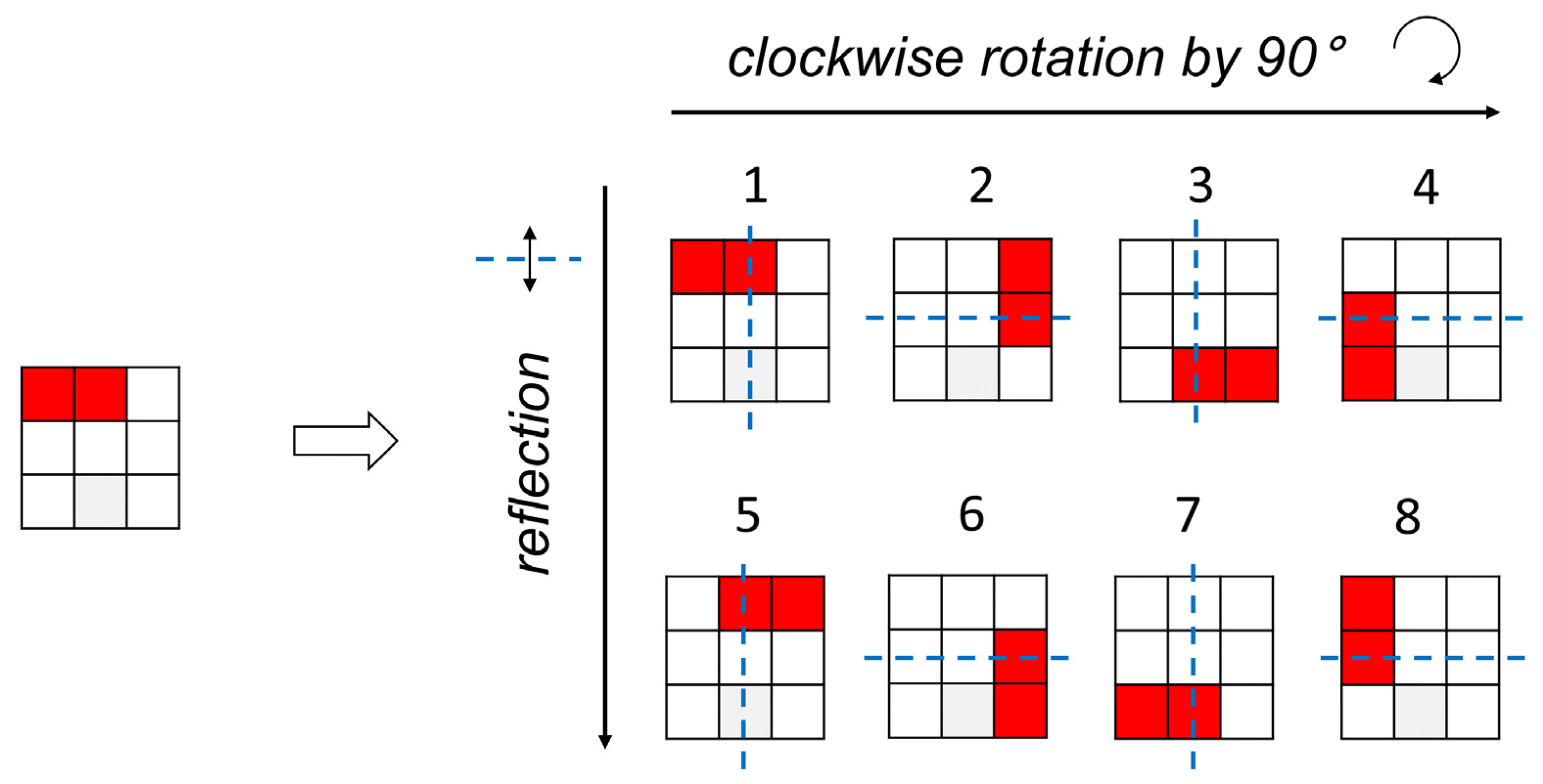
In the N × N square reactant model of the first type, to study the effects of the size, number, and arrangement of reactive patches on the kinetics, we first consider various N × N patch configurations generated by the model. Since the N × N square model has N × N cells and each cell can be a reactive patch or not, the total number of configurations for the N × N square model is . For instance, for N = 2 and 3, the total number is and , respectively. In fact, in this work, we completely analyze all the configurations for N = 2, 3, applying symmetric operations to the configurations. Note that a configuration of reactive patches can generate eight kinetically equivalent configurations by rotations and reflections through planes, as shown in Figure 3. However, when the configuration has symmetries in the arrangement of patches, the number of configurations generated is reduced because some configurations are duplicated. Therefore, we consider only symmetrically representative configurations with the number of equivalent configurations .
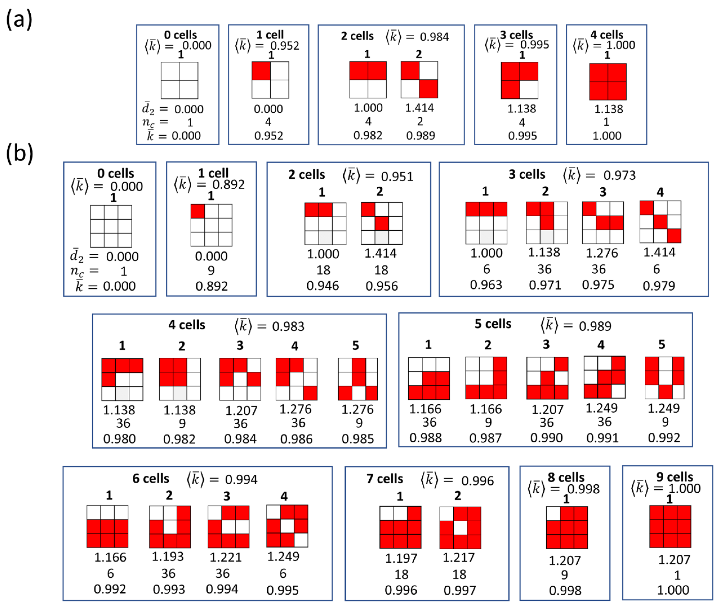
In Figure 4, we present all the symmetrically representative configurations of patches for N = 2 and 3 and the normalized rate constants calculated from the solutions of the Smoluchowski equations. Since the rate constant is dependent on the distances between the reactive patches (cells), we calculate the average of the distances between all pairs of the reactive cells . Note that a similar study based on the geometric mean pair distance between patches has been performed [17]. The average pairwise distances are also displayed in Figure 4. Here, we find a general trend that as increases, the normalized rate constant increases. Therefore, for a given number of reactive cells, the normalized rate constant could differ depending on the distances between the patches or the configurations of the patches. Notably, in the 3 × 3 square model, the configurations giving the highest rate constant are mainly the configurations that have a symmetric arrangement of the reactive patches (configurations 8, 23, 22, 16, and 3 for 2, 4, 5, 6, and 8 reactive cells, respectively).
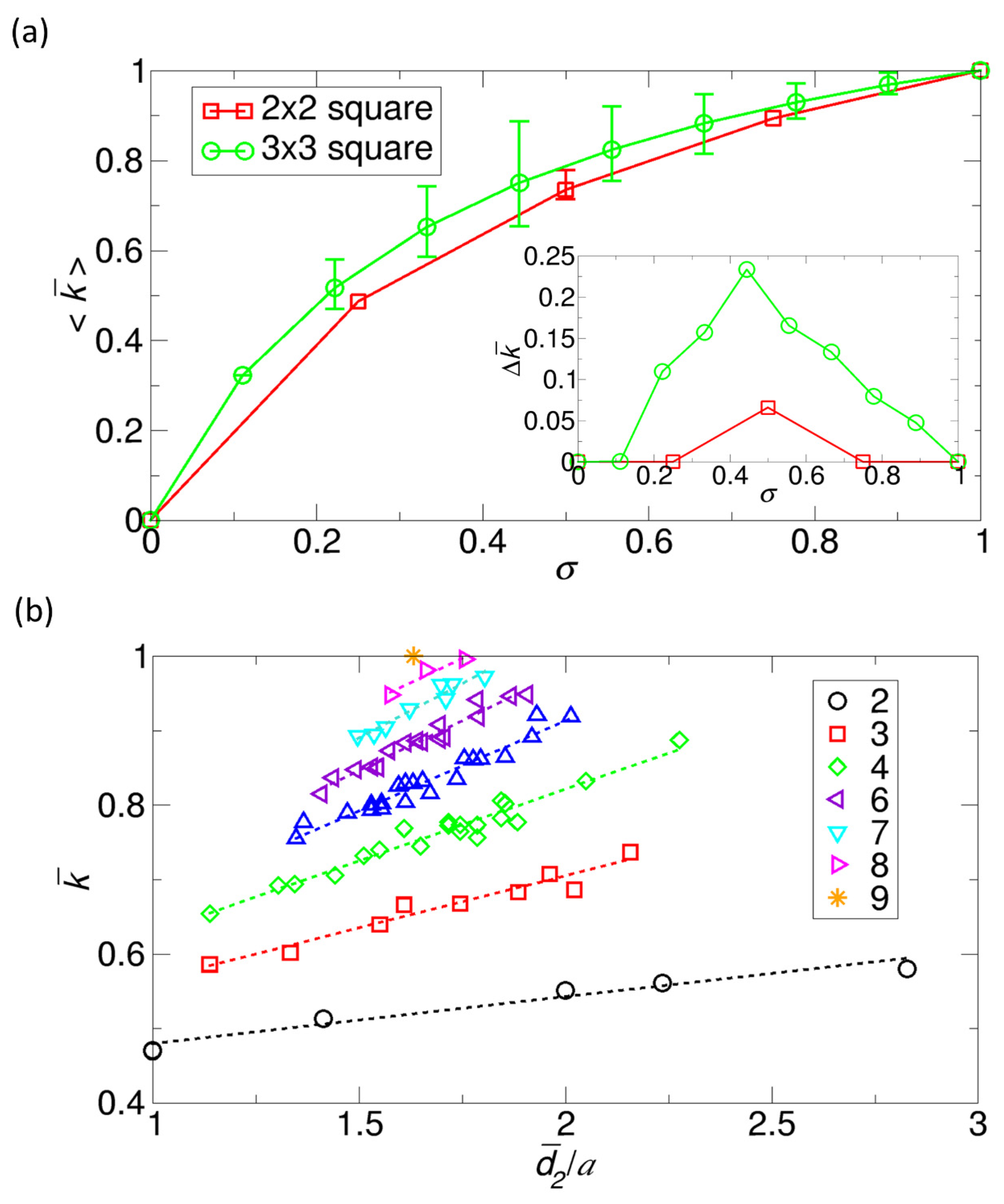
Additionally, we calculate the ensemble-averaged value of the normalized rate constants for a given number of reactive cells, since we can determine the probability of each representative configuration from . From the calculation, we plot the ensemble-averaged rate constant against the surface coverage ratio of reactive cells over the entire reactant area . is easily calculated by counting the number of reactive cells; for example, in the 2 × 2 model, if only one cell is reactive, is 0.25 because it is 1 over 4. The plot is shown in Figure 5a. As one can expect, as increases, the normalized rate constant increases, but as approaches 1, the slope of the rate constant against decreases, which is due to the increase in the competition between reactive patches. We also show the maximum and the minimum values of the normalized rate constant for a given value of . Interestingly, as is shown in the inset of Figure 5a, the variation in the rate constant , i.e., the difference between the maximum and minimum values increases at low values of , reaches its maximum, and then decreases at large values. This characteristic behavior was also observed in the reactive patches of a spherical reactant [7,17].
Another feature from Figure 5a is that for a given value of , the ensemble-averaged normalized rate constant for the 3 × 3 model is larger than that for the 2 × 2 model. This outcome is consistent with the observation in a spherical reactant that a smaller patch gives a larger rate constant [7,17]. Basically, this occurrs because in the case of a higher value of N, more configurations exist in which the reactive patches are separated, which reduces the competition between patches. Therefore, one can expect that as N increases in the N × N model, one can obtain a higher ensemble-averaged rate constant.
In this work, we plot the normalized rate constant as a function of the dimensionless distance , where is the length of the unit cell. The result is shown in Figure 5b. Since the cases of the 2 × 2 square model are trivial, we present only the cases of the 3 × 3 square model. From the plot, we find a general trend that as increases, the normalized rate constant increases. Specifically, from linear regressions, the result shows that a strong correlation exists between the normalized rate constant and , but the linear lines are not monotonously increasing, which means that is a good parameter but is not a perfect parameter for evaluating the competition between reactive patches in a given configuration.
3.2. Second Model Type: N × N Square Reactant Model
The main difference between the first and the second model types comes from whether PBCs are applied to the x and y dimensions. In this section, we discuss the second model type with PBCs. When we apply PBCs to the x-y plane, the number of symmetrically representative configurations that we have to consider is significantly reduced, as shown in Figure 6. As in Figure 4, we calculate , , and for each representative configuration for the 2 × 2 and 3 × 3 square models. For a given number of reactive cells, we arrange the configurations in increasing order of . As expected, the normalized rate constant generally increases with .
The ensemble-averaged normalized rate constant is shown in Figure 7a. We also observe that as increases, the rate constant increases, which is the same trend observed in Figure 5a. However, differences exist. Notably, the normalized rate constant is very high even at low values of . That is, even a small surface coverage of reactive patches can produce a high rate constant. This significant increase due to the boundary condition is discussed further with the dependence of the kinetics on in Section 3.3. Another noticeable property from Figure 7a is that the variation in the rate constant is small, as indicated in the inset of Figure 7a. These interesting properties with the PBCs were also found in the reaction systems of a spherical reactant with multiple reactive patches [10]. For a spherical reactant, small patches can produce a large rate constant, and the distribution of rate constants is narrow, which means that the difference between the maximum and minimum values is relatively small. These common features may come from the fact that the reactant surface with PBCs in the second model type is topologically similar to the surface over a sphere in that they are closed surfaces and have no boundary; if one walks straight starting from a certain position on the surface, one will eventually return to the starting position. As in Figure 5b, we also show a scatter plot of the normalized rate constant and the dimensionless average pairwise distance for symmetrically representative configurations in the 3 × 3 square reactant model. The linear regression lines show a strong correlation between them.
3.3. Dependence of Kinetics on the Fraction of the Total Reactive Patch Area
The results of the N × N square reactant models in Section 3.1 and Section 3.2 indicate that the normalized rate constant is apparently dependent on the fraction of the total area of the reactive patches . For example, let us consider the first model type without PBCs. From Figure 4, if we consider Case 1 of the 3 × 3 model with one reactive cell (), Case 1 of the 2 × 2 model with one reactive cell (), Case 1 of the 3 × 3 model with four reactive cells (), and Case 1 of the 2 × 2 model with four reactive cells (), we understand the dependence of kinetics on in that the rate constant for a single square increases in a nonlinear way as increases; = 0 (), 0.323 (), 0.486 (), 0.654 (), and 1 () (see the filled squares in Figure 8). Similarly, for the PBC cases, from Figure 6, if we consider Case 1 of the 3 × 3 model with one reactive cell (), Case 1 of the 2 × 2 model with one reactive cell (), Case 2 of the 3 × 3 model with four reactive cells (), and Case 1 of the 2 × 2 model with four reactive cells (), we see that the rate constant increases with in another nonlinear way; = 0 (), 0.892 (), 0.952 (), 0.982 (), and 1 () (see the filled circles in Figure 8).
However, because of the limitations in exploring various cases with different values of from the 2 × 2 and 3 × 3 square reactant models, we consider another square reactant model in which one reactive square cell is placed at the center of the square reactant. Here, we change the size of the reactive cell, such that we have different values of . The result is shown in Figure 8. We see that this result from the square model with one reactive cell is consistent with the results from the N × N square model from Figure 4 and Figure 6 (filled symbols). The main feature is that as increases, the normalized rate constant increases, and the effect is much more significant with PBCs. That is, for a given value of , the rate constant in the presence of PBCs is larger than the corresponding rate constant without PBCs. In the presence of PBCs, even with = 0.01, the normalized rate constant is 61.7% of the maximum rate constant with = 1, while the corresponding rate constant in the first model type without PBCs is 9.78%. Additionally, we notice that in the inset of Figure 8, the concentration color at = 0.1 is almost blue (concentration is near zero) for the case with PBCs; in this case, the normalized rate constant is 88.2% of the maximum rate constant.
The high rate constants obtained with PBCs may suggest that in the first type of model, even in a single small patch in a reactant, if one breaks it into many smaller patches and arranges them such that any patch looks like the one with PBCs in Figure 8, the overall rate constant can be significantly increased. To check this idea, we consider the division-separation procedure of reactive cells in Section 3.5 and Section 3.6 to see how the procedure enhances the rate constant.
Additionally, from the agreement of between the square model of a single reactive cell and the 2 × 2 and 3 × 3 square models in Figure 8, we note that the 2 × 2 and 3 × 3 square models are useful in obtaining a general trend of the dependence of the kinetics on , although the results do not cover the full range of . This result confirms the validity and usefulness of the simple N × N square reactant models.
3.4. Effect of the Reactive Patch Distribution on the Kinetics
The results of the N × N models in Section 3.1 and Section 3.2 show that the rate constant is dependent on the distribution of the reactive patches, as demonstrated by the variation in the rate constant at a fixed value of in the insets of Figure 5a and Figure 7a. The general trend is that when the patches (cells) are aggregated, the normalized rate constant is lower than when the patches are largely separated. Here, we notice that the variation in the rate constant is dependent on the fraction of the area of the unit cell in the N × N model. That is, as N increases, decreases, which allows more diverse arrangements of patches on a reactant and increases the variation of the rate constant. Note that in the 2 × 2 square reactant model, is 1/4 and in the 3 × 3 model, is 1/9.
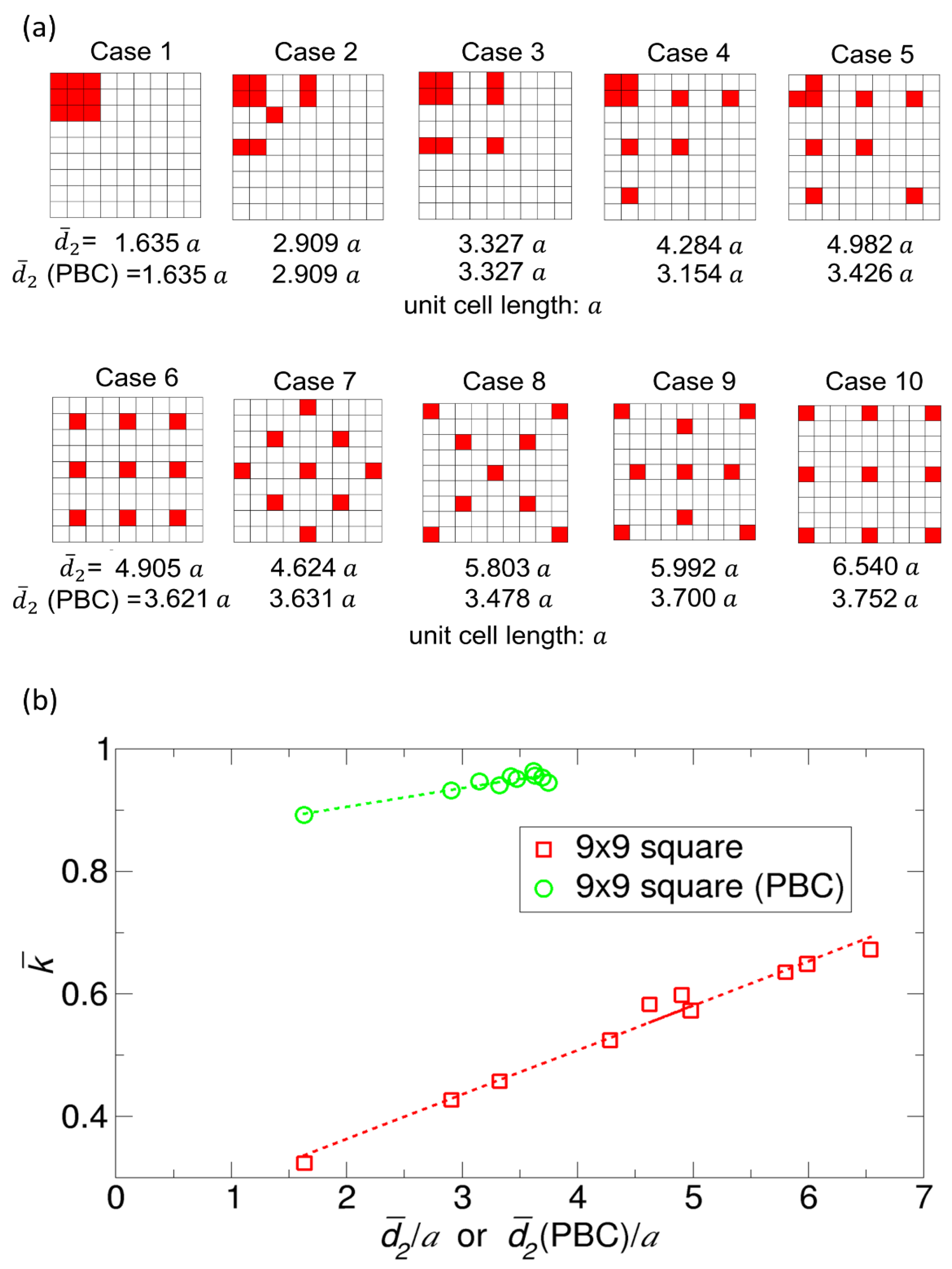
Since the 2 × 2 and 3 × 3 square reactant models do not provide a variety of patch arrangements, we consider the spatial arrangements of patches with = 1/9 in the 9 × 9 square model with = 1/81. In this case, the number of reactive cells is 9. Note that in the 3 × 3 square model, the number of reactive cells corresponding to = 1/9 is 1. Moreover, note that in contrast to the 2 × 2 and 3 × 3 square models, in this case, considering all the possible patch configurations is practically impossible because the total number of arrangements of patches is enormous; when we ignore symmetrically equivalent patch arrangements and PBCs, the number of patch configurations is 81C9; in fact, when we consider the symmetry of arrangements and PBCs, the actual number of symmetrically unique patch configurations is less than this number. Therefore, instead of considering all the cases, we consider 10 representative cases from the one with mostly aggregated patches to the one with largely separated patches, as shown in Figure 9a. We also use the average value of the pairwise distance as a way to measure the degree of scattering of patches over the reactant surface. For each case, we calculate the normalized rate constant for the first and second model types. We display the results as a plot of the normalized rate constant versus the dimensionless average pairwise distance or , as shown in Figure 9b.
In Figure 9b, as one can expect from the competition between patches, as the reactive cells move away from each other or increases, the normal rate constant increases. This effect is more apparent in the first type of model without PBCs. Interestingly, for a given value of = 1/9, by simply redistributing patches from the most aggregated patches (Case 1) to the maximally separated patches (Case 10), we can increase the normalized rate constant by more than two times, from 0.323 to 0.671; the normalized rate constant in Case 10 ( = 1/9) is comparable to the ensemble-averaged rate constant for three reactive cells (= 1/3) in the 3 × 3 model (see Figure 4b; 0.653). Therefore, in addition to increasing the value, another way to increase the rate constant is to arrange the patches such that they are more separated from each other.
In the second type of model with PBCs, we also observe the trend that the rate constant increases with , as is indicated by the linear regression line. However, with PBCs, except for Case 1 (the most aggregated case), the normalized rate constant does not strongly depend on the details of the patch arrangements in that the values of are more or less the same. Another interesting observation is that the case giving the highest rate constant is Case 6 (the most symmetrical arrangement), where the reactive cells are uniformly distributed in the presence of PBCs with equal distance between neighboring cells. This arrangement of reactive cells corresponds to the symmetric distribution minimizing their competitions in a sphere, which is related to the solutions of the Thomson problem or the Tammes problem [7]. Specifically, our competition-minimization problem with n reactive patches is similar to the Thomson problem aimed to find the spatial arrangement of n electrons on a sphere giving the minimum potential energy and the Tammes problem aimed to find the spatial arrangement of circles maximizing the minimal distance between circles in that their solutions are generally uniformly distributed arrangements.
3.5. Symmetric Reactive Patch Distributions
Based on the effect of the patch distribution in Section 3.4, we further study the dependence of normalized rate constant on the number of reactive patches for a given value of . For this study, we employ the square reactant models of = 1/9 with symmetric patch distributions, in which the patches are uniformly distributed over the reactant surface (see Case 6 of Figure 9a). In the patch distributions, we consider = 12, 22, 32, 42, 52, 62, 72, and 82 and arrange the patches symmetrically (see Figure 10a). Note that the case with = 32 is exactly the same as Case 6 of Figure 9a. For each case, we calculate the normalized rate constants for the first and second model types, the results of which we present in Figure 10b. The general trend is that the normalized rate constant increases with . As a result, for the first type of model, the case with 82 and = 1/9 has a high rate constant (0.807), comparable to the rate constant (0.827) of the case with 1 and = 0.7 (see Figure 8). However, for the second type of model, even for 1, the normalized rate constant is very high (0.891); thus, the enhancement of due to the division and separation of patches is not as dramatic as that in the first type of model. Another feature in the plots of Figure 10b is that as increased, the effect of the enhancement of is reduced; the enhancement is largest when changed from 1 to 4.
3.6. Multiple Divisions of Patches and the Power–Law Relationship
For the square reactant model with symmetric patch distributions in Section 3.5, we can further discuss the mathematical relationship between the normalized rate constant and the number of reactive patches for the cases with a fixed value of . For the discussion, we consider sequential construction procedures for systematically generating the reactants with symmetric patch distributions of smaller patches. Precisely speaking, the procedures consist of N steps of division and symmetric arrangement of patches, and the procedures are sequential in that the reactant at the Mth step is obtained from the reactant at the previous M-1th step.
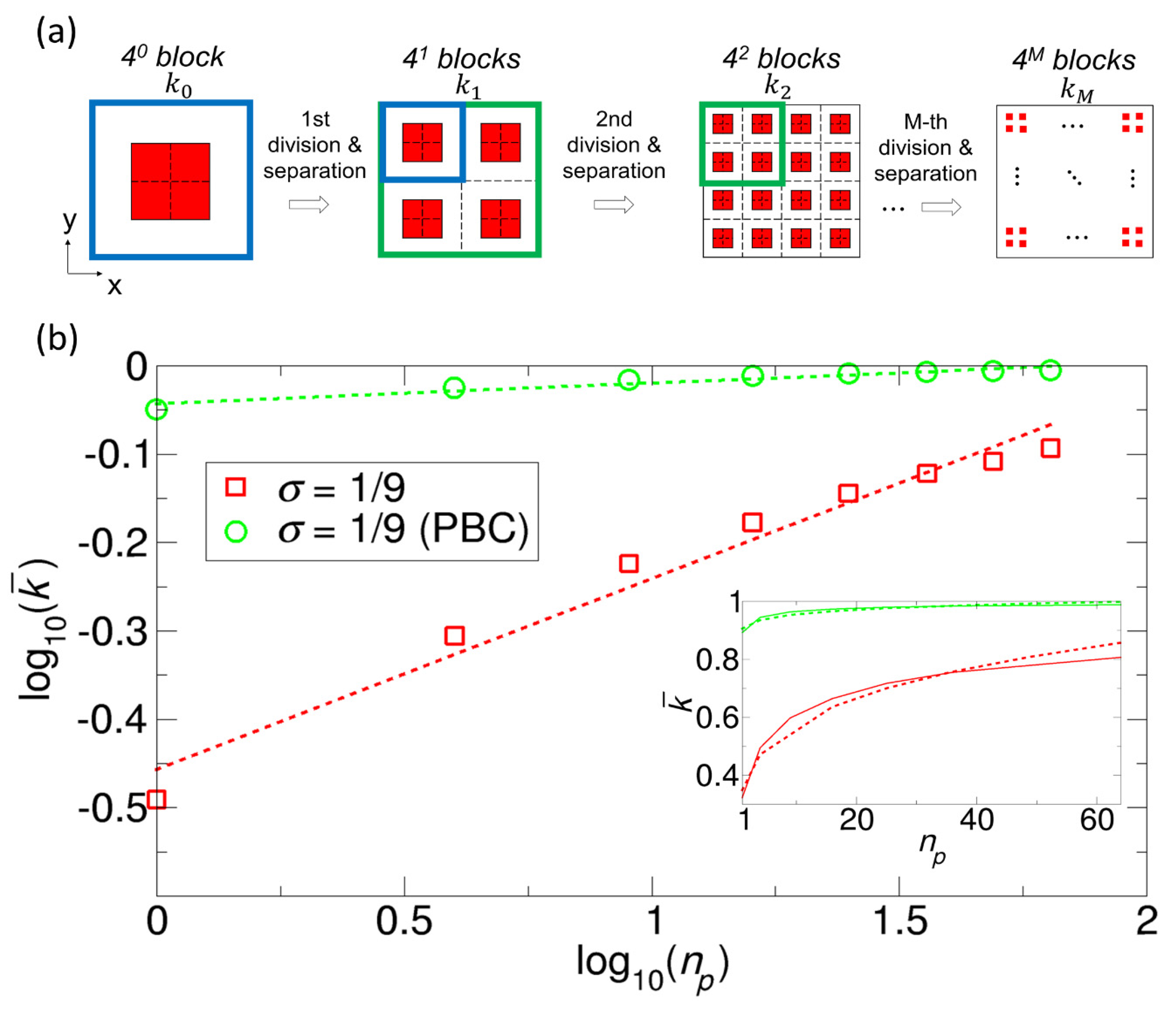
To explain the procedure in detail, we start with a single square reactive patch at the center of the square reactant, as shown in the leftmost reactant in Figure 11a. In the first step, we divide the square reactive patch into four equal smaller patches. In Figure 11a, the division of the patch is represented by the dotted lines. We also perform the same type of division for the entire square reactant, resulting in four smaller square blocks. For each smaller square block, we place one reactive patch at the center of the square block, resulting in the separation of the original reactive patch. The patch distribution obtained from this procedure is shown in the second reactant in Figure 11a, which corresponds to the symmetric patch distribution with = = in Figure 10a. Note that each block with a smaller reactive patch has exactly the same shape as that of the original initial reactant. That is, if we select any one of the four blocks in the second reactant and enlarge its area by four times, the enlarge block will be exactly the same as the original reactant (see the blue square lines in Figure 11a). Now, if we apply the same division-separation procedure to each of the four blocks in the second reactant in Figure 11a, we generate another four smaller blocks for each block. As a result, the total number of patches is = =; the overall patch distribution is shown in the third reactant in Figure 11a. We can repeatedly apply this procedure to a reactant at each step.
Now, we consider how the overall normalized rate constant changes as we carry out the procedure repeatedly. For a quantitative discussion on the change in the rate constant due to the first division-separation procedure, we denote the rate constant before the procedure as , the rate constant after the procedure as , and the overall increasing factor of the rate constant due to the reduction in the competition by the first procedure as . Then, the overall rate constant is , where . Note that if the rate constant of each patch is simply proportional to its area, the overall rate constant is , since there are four patches with a rate constant of . Therefore, the reduction in competition is taken into account only through the factor , which may be different from system to system.
Similarly, from the second division-separation procedure, the competitions among the patches are further reduced. After the second procedure, we obtain the third patch distribution, in which 16 identical blocks are generated. Each block has a reactive square patch at its center. Because of the way we construct the reactant, a similarity symmetry exist between a four-block square in the third patch distribution and a four-block square (entire reactant) in the second patch distribution (see the green square lines in Figure 11a). Because of the similarity symmetry appearing in the sequential procedures, we may assume that the increasing factor due to the reduction in the competition by the second procedure is the same as the increasing factor by the first procedure. Under the assumption that , the overall rate constant after two divisions, or , can be written as . Together with , we finally obtain .
In this way, we can repeat the division-separation procedure under the similarity symmetry, the competition is continuously reduced, and as a result, the overall rate constant increases. Moreover, with the assumption that is constant, after an M-fold symmetric division and arrangement, we finally obtain the overall rate constant . That is, we obtain the power–law relationship between the rate constant and the number of division-separation procedures . Subsequently, we obtain the normalized rate constant , which is calculated by dividing by the rate constant for ( or ), and the same power law , where . However, note that this power–law scaling behavior has limitations. That is, we consider only the nearest neighbor competitions through the similarity symmetry, but if we take into account the competitions arising from all possible pairs of patches, the behavior of the rate constant will deviate from the power–law behavior as M or increases. Moreover, since the upper value of is 1 (normalized rate constant for ), we expect that as the number of procedures M increases, will eventually become saturated, which means that decreases; otherwise diverges as M increases.
In the case above of the division of patches by four, since the number of patches and the number of procedures are related by , we can represent in terms of as . That is, , which means that is proportional to . Additionally, note that from a logarithmic property, we can rewrite as . Therefore, the simple scaling argument provides a power law of for the rate constant , generally denoted by .
3.6.1. Analysis for the Case of 1/9
For the reactants with symmetric distributions in Figure 10a, to see what the plot of versus looks like according to the above division-by-four procedure, we calculate for the rate constant shown in Figure 10b and display the log-log plot in Figure 11b. In the plot, the y-intercept and the slope correspond to and , respectively. Again, the physical interpretation of slope () as means that if we increase by times (e.g., = 1, 4, 16, 64, …), the increasing factor is given by . However, the trend deviates from linearity as increases. In fact, to find the slope, we fit the data with a linear equation for versus using the xmgrace program. The correlation coefficients for the first and the second model types in Figure 10 are 0.985 and 0.960, respectively. These high values explain why the relation between and can be described by power laws ( or ). From the linear equations for the regressions, we can easily determine for the division-by-four procedure; for a determined value of , is given by . Note again that here, the factor of is due to the division by four carried out in the procedure. In general, if we break a patch into smaller patches at every step of the division, . In this case, when each patch was divided into patches in the procedures, indicate how the normalized rate constant scales with (=).
In fact, from Figure 11b, we find power laws for by determining the values of and ; the slopes are 0.2158 and 0.02348 for the first and second model types, respectively, and accordingly, the values are 1.349 and 1.033, respectively. In fact, in the inset of Figure 11b, we plot the normalized rate constants calculated by the power laws of (dashed lines), along with the original ones shown in Figure 10b (solid lines). The two curves are generally in good agreement, but the rate constant from the power–law deviates from the original rate constant as increases.
Instead of using four patches in the division-separation procedure, we can break a single patch into a smaller number of patches. In this case, decreases since the competition decreases less; for example, in a division-by-two procedure, the values () for the first and second model types are 1.161 and 1.016, respectively. In contrast, if we break the patch into a larger number of patches, will increase since the competition decreases more. For example, in a division-by-eight procedure, the values () for the first and second model types are 1.566 and 1.050, respectively.
We now consider the general properties of the power laws observed in Figure 11b. First, for all cases, is greater than 1, which means that always increases when the division and separation take place. Second, as increases, we expect that the slope () decreases and eventually becomes zero () since has an upper bound of 1; otherwise, would be larger than 1 as increases.
3.6.2. Analysis for the Cases of 0.01 and 0.001
In a reactant with symmetrically distributed reactive patches, we expect that as increases, the interference between a reactive patch and its other patches beyond the nearest neighboring patches is more significant. As a result, the increasing factor is more dependent on the number of patches, which means that the assumption that is constant, used to derive the power law of , becomes questionable.
In contrast, if decreases, the interference is less significant and the assumption that the increasing factor is constant makes more sense. To see if shows more of a power–law behavior for small values of , we consider the case of = 0.01 for a reactant with symmetrically distributed patches for the first and second model types. The result is shown in Figure 12. We also consider the case of = 0.001, but it is only for the second type of model; moreover, we calculate the normalized rate constant only up to = 25 because of the difficulty in creating a very refined mesh for the first and second model types. In Figure 12a, we display the normalized rate constant as a function of and in Figure 12b, we show the log-log plot of against . Remarkably, the correlation coefficient for the case of the first model type with = 0.01 is very high (0.997). In fact, the correlation coefficients for other cases are also high; 0.970 and 0.988 for the second model type with = 0.01 and 0.001, respectively. From the slopes, we also determine the values for the division-by-four procedure, i.e., 1.723 (first type, = 0.01), 1.1494 (second type,= 0.01), and 1.448 (second type,= 0.001).
4. Conclusions
In this work, we considered the diffusion-limited reactions between reactive patches on a reactant molecule fixed on a plane (x-y plane) and point-like partner reactant molecules and studied how the size, number, and spatial arrangement of reactive patches affect the overall reaction kinetics. For a systematic study, we proposed discrete N × N square reactant models, where the reactive patches are squares and are on the surface of a square reactant with an N × N grid; the patches occupy some of the N × N cells generated by the grid lines. Furthermore, we considered two types of reaction model. In the first model type, a reactant is placed on a chemically inert plane, and in the second, reactive patches are periodically placed on the entire reactant plane. Therefore, in the second type of model, we applied PBCs to the x and y coordinates.
For the 2 × 2 and the 3 × 3 square reactant models, we examined all possible cases of reactive patches from = 0 (non-reactive) to = 1 (fully reactive), where is the ratio of the total reactive patch area to the total reactant area. Through a complete study of the kinetics for the models, we found that as increases, the rate constant increases, but because of large competitions between patches, at large values, the increasing rate decreases. Additionally, we noticed that for a given value of , large variations in the rate constant could occur due to various arrangements of the reactive patches. This observation signifies that by rearranging patches, we may increase the rate constant. By comparing the ensemble-averaged rate constants in the 2 × 2 and 3 × 3 models, we see that for a given value of , the ensemble-averaged rate constant for the 3 × 3 model is larger than that for the 2 × 2 model, because, with smaller reactive patches, we can generate more patch arrangements that result in less competition between patches than with larger patches.
Additionally, using a 9 × 9 model with = 1/9, we investigated the effect of the patch distribution on the kinetics by considering ten representative patch distributions. As one expects, when the patches are aggregated, the overall normalized rate constant is small, but when they are largely separated, the rate constant is large. In fact, for both the first and second model types, the patch distribution giving the lowest value of is the one where all reactive patches are maximally aggregated or compact. However, the patch distributions giving the highest value are different; the patch distribution for the first model type is the symmetric distribution where the reactive patches are maximally separated from each other (Case 10 in Figure 9a), and the patch distribution for the second model type is the symmetric distribution where the patches are uniformly distributed, and all the distances between nearest neighbors (including the PBC neighbors) are the same (Case 6 in Figure 9a). Interestingly, the latter patch distribution is similar to the uniform patch distribution in a sphere, maximizing the overall rate constant.
By further developing the idea of the symmetric patch distribution, we proposed a method to systematically increase the overall rate constant for a given value of by breaking a patch into smaller patches and separating them symmetrically based on the uniform arrangement of patches (Case 6 in Figure 9a). When we applied this division-separation procedure multiple times, we showed that the rate constant significantly increases, especially in the first type of model. Interestingly, we found that a power–law relationship exists between the normalized rate constant and the number of patches , and the relationship is more accurate when is smaller.
One possible future research direction of this work is to show the usefulness of our discrete square reactant models. In this work, the ensemble used for calculating the averages is a microcanonical ensemble since we assume the probability of each configuration of patches being the same, meaning that the patches do not interact with each other. However, when the patches interact with themselves attractively or repulsively, the probability of each configuration depends on the arrangement of patches; thus, we may need to consider a canonical ensemble based on the potential energy of patches, which may be more realistic and more interesting. In that case, compared to continuous models, our discrete N × N square models are beneficial in that the number of patch configurations to be considered is finite, not infinite. Therefore, the study of the kinetics with the interactions between patches using our discrete models will be the subject of future investigations.
Funding
This work was supported by the National Research Foundation of Korea (NRF) grant funded by the Korea government (MSIT) (No. 2020R1F1A1070163) and the Hankuk University of Foreign Studies Research Fund of 2020.
Conflicts of Interest
The author declares no conflict of interest.
References
- Samson, R.; Deutch, J.M. Exact solution for the diffusion controlled rate into a pair of reacting sinks. J. Chem. Phys. 1977, 67, 847. [Google Scholar] [CrossRef]
- Eun, C.; Kekenes-Huskey, P.M.; McCammon, J.A. Influence of neighboring reactive particles on diffusion-limited reactions. J. Chem. Phys. 2013, 139, 07B623_1. [Google Scholar] [CrossRef] [PubMed]
- Ivanov, K.L.; Lukzen, N.N. Diffusion-influenced reactions of particles with several active sites. J. Chem. Phys. 2008, 128, 04B616. [Google Scholar] [CrossRef] [PubMed]
- Strieder, W. Interaction between two nearby diffusion-controlled reactive sites in a plane. J. Chem. Phys. 2008, 129, 134508. [Google Scholar] [CrossRef] [PubMed]
- Kang, A.; Kim, J.-H.; Lee, S.; Park, H. Diffusion-influenced reactions involving a reactant with two active sites. J. Chem. Phys. 2009, 130, 03B606. [Google Scholar] [CrossRef] [PubMed]
- Berezhkovskii, A.M.; Dagdug, L.; Lizunov, V.A.; Zimmerberg, J.; Bezrukov, S.M. Communication: Clusters of Absorbing Disks on a Reflecting Wall: Competition for Diffusing Particles; American Institute of Physics: College Park, MD, USA, 2012. [Google Scholar]
- Eun, C. Effects of the Size, the Number, and the Spatial Arrangement of Reactive Patches on a Sphere on Diffusion-Limited Reaction Kinetics: A Comprehensive Study. Int. J. Mol. Sci. 2020, 21, 997. [Google Scholar] [CrossRef] [PubMed] [Green Version]
- Berg, H.C.; Purcell, E.M. Physics of chemoreception. Biophys. J. 1977, 20, 193–219. [Google Scholar] [CrossRef] [Green Version]
- Shoup, D.; Szabo, A. Role of diffusion in ligand binding to macromolecules and cell-bound receptors. Biophys. J. 1982, 40, 33–39. [Google Scholar] [CrossRef] [Green Version]
- Northrup, S.H. Diffusion-controlled ligand binding to multiple competing cell-bound receptors. J. Chem. Phys. 1988, 92, 5847–5850. [Google Scholar] [CrossRef]
- Zwanzig, R. Diffusion-controlled ligand binding to spheres partially covered by receptors: An effective medium treatment. Proc. Natl. Acad. Sci. USA 1990, 87, 5856–5857. [Google Scholar] [CrossRef] [Green Version]
- Berezhkovskii, A.M.; Makhnovskii, Y.A.; Monine, M.I.; Zitserman, V.Y.; Shvartsman, S.Y. Boundary homogenization for trapping by patchy surfaces. J. Chem. Phys. 2004, 121, 11390–11394. [Google Scholar] [CrossRef] [PubMed] [Green Version]
- Lu, S.-Y. Patch size effect on diffusion and incorporation in dilute suspension of partially active spheres. J. Chem. Phys. 2004, 120, 3997–4003. [Google Scholar] [CrossRef]
- Makhnovskii, Y.A.; Berezhkovskii, A.M.; Zitserman, V.Y. Homogenization of boundary conditions on surfaces randomly covered by patches of different sizes and shapes. J. Chem. Phys. 2005, 122, 236102. [Google Scholar] [CrossRef] [PubMed]
- Berezhkovskii, A.M.; Monine, M.I.; Muratov, C.B.; Shvartsman, S.Y. Homogenization of boundary conditions for surfaces with regular arrays of traps. J. Chem. Phys. 2006, 124, 036103. [Google Scholar] [CrossRef] [Green Version]
- Lindsay, A.E.; Bernoff, A.J.; Ward, M.J. First passage statistics for the capture of a Brownian particle by a structured spherical target with multiple surface traps. Multiscale Modeling Simul. 2017, 15, 74–109. [Google Scholar] [CrossRef] [Green Version]
- Wu, J.-C.; Lu, S.-Y. Patch-distribution effect on diffusion-limited process in dilute suspension of partially active spheres. J. Chem. Phys. 2006, 124, 024911. [Google Scholar] [CrossRef]
- Bernoff, A.J.; Lindsay, A.E. Numerical approximation of diffusive capture rates by planar and spherical surfaces with absorbing pores. SIAM J. Appl. Math. 2018, 78, 266–290. [Google Scholar] [CrossRef] [Green Version]
- Eun, C. Theory of curvature-dependent kinetics of diffusion-limited reactions and its application to ligand binding to a sphere with multiple receptors. J. Chem. Phys. 2018, 149, 024102. [Google Scholar] [CrossRef]
- Ridgway, W.J.; Cheviakov, A.F. Locally and globally optimal configurations of N particles on the sphere with applications in the narrow escape and narrow capture problems. Phys. Rev. E 2019, 100, 042413. [Google Scholar] [CrossRef] [Green Version]
- Grebenkov, D.S. Diffusion toward non-overlapping partially reactive spherical traps: Fresh insights onto classic problems. J. Chem. Phys. 2020, 152, 244108. [Google Scholar] [CrossRef]
- Lawley, S.D. Boundary homogenization for trapping patchy particles. Phys. Rev. E 2019, 100, 032601. [Google Scholar] [CrossRef] [PubMed]
- Plunkett, C.E.; Lawley, S.D. Bimolecular binding rates for pairs of spherical molecules with small binding sites. arXiv 2020, arXiv:2002.11703. [Google Scholar]
- Berezhkovskii, A.M.; Dagdug, L.; Lizunov, V.A.; Zimmerberg, J.; Bezrukov, S.M. Trapping by clusters of channels, receptors, and transporters: Quantitative description. Biophys. J. 2014, 106, 500–509. [Google Scholar] [CrossRef] [PubMed] [Green Version]
- Eun, C. Effect of surface curvature on diffusion-limited reactions on a curved surface. J. Chem. Phys. 2017, 147, 184112. [Google Scholar] [CrossRef] [PubMed]
- Frenkel, D.; Smit, B. Understanding Molecular Simulation: From Algorithms to Applications; Elsevier: Amsterdam, The Netherlands, 2001; Volume 1. [Google Scholar]
Figure 1.
Schematic diagram of our first chemical reaction model. (Left) One reactant molecule A with an N × N cellular surface (black lines) is located at the center of the coordinate system and is on the x-y plane at z = 0. The outer boundary condition is represented by the blue lines. (Right) The concentration profiles of reactant B from the Smoluchowski solutions for the N × N square models of N = 2 and 3 with certain reactive cell distributions are represented by color maps. The length of each side of reactant A is 1.8 (: Unit length), and the distance from the center to the outer boundary (Router) is 10 . The red cells in the N × N square reactants indicate the reactive patches.

Figure 2.
Schematic diagram of our second chemical reaction model. (Center) The arrangement of reactive patches on the bottom surface at z = 0 is repeated through periodic boundary conditions (PBCs) for the x-y dimensions. The blue top surface at z = corresponds to the outer boundary in the first model type in Figure 1, and the concentration on the blue surface is normalized to 1. (Left) The concentration profile of reactant B obtained from the Smoluchowski solution for the 3 × 3 square model with a certain reactive cell distribution is represented by a color map. (Right) The concentration profile of reactant B for the 2 × 2 square model with a certain reactive cell distribution is represented. In this unit cell, the length of each side of the bottom surface at z = 0 is 1.8 (: Unit length), and the distance from the bottom surface to the top surface () is 10 . The red cells in the N × N square reactants indicate the reactive patches.

Figure 3.
Eight configurations are generated from the configuration of reactive patches are shown on the left by symmetric operations of rotations around the z-axis out of the page and reflections through the planes represented by the dotted lines.
Figure 3.
Eight configurations are generated from the configuration of reactive patches are shown on the left by symmetric operations of rotations around the z-axis out of the page and reflections through the planes represented by the dotted lines.

Figure 4.
(a) Average pairwise distance between reactive patches (cells) (), the number of all configurations kinetically equivalent to a representative configuration (), and the normalized rate constant () of a representative configuration in the 2 × 2 square model of the first type. All representative configurations from 0 cells (no reactive) to 4 cells (full reactive) are considered. (b) , , and of a representative configuration in the 3 × 3 square model of the first type. All representative configurations from 0 cells (no reactive) to 9 cells (full reactive) are considered. For a given number of reactive cells, we arrange the configurations in order of increasing . Note that the unit of is the length of unit cell of the N × N square model. represents the ensemble-averaged value of for a given number of reactive cells.

Figure 5.
(a) Ensemble-averaged normalized rate constant as a function of the fraction of reactive cells over the entire reactant surface area () for the 2 × 2 and 3 × 3 square reactant models of the first type. is easily calculated by the number of reactive cells over the total number of cells. (b) For the numbers of reactive cells from two to nine in the 3 × 3 square model, the plot of the normalized rate constant () versus the dimensionless average pairwise distance (, which is the average pairwise distance () over the length of the unit cell (). The dotted lines represent linear regression lines obtained from the xmgrace program. In the linear regressions, the correlation coefficients are 0.972 (2 cells), 0.978 (3 cells), 0.977 (4 cells), 0.974 (5 cells), 0.978 (6 cells), 0.971 (7 cells), and 0.968 (8 cells).

Figure 6.
(a) Average pairwise distance between reactive patches (cells) (), the number of all configurations kinetically equivalent to a representative configuration (), and the normalized rate constant () of a representative configuration in the 2 × 2 square model of the second type with PBCs. All representative configurations from 0 cells (no reactive) to 4 cells (full reactive) are considered. (b) , , and of a representative configuration in the 3 × 3 square model of the second type with PBCs. All representative configurations from 0 cells (no reactive) to 9 cells (full reactive) are considered. For a given number of reactive cells, we arrange the configurations in order of increasing . Note that the unit of is the length of unit cell of the N × N square model. represents the ensemble-averaged value of for a given number of reactive cells.

Figure 7.
(a) Ensemble-averaged normalized rate constant as a function of the fraction of reactive cells over the entire reactant surface area () for the 2 × 2 and 3 × 3 square models of the second type with PBCs. is easily calculated by the number of reactive cells over the total number of cells. (b) For numbers of reactive cells from two to nine in the 3 × 3 square model with PBCs, the plot of the normalized rate constant () versus the dimensionless average pairwise distance (, which is the average pairwise distance () over the length of the unit cell () in the presence of PBCs. The dotted lines represent linear regression lines obtained from the xmgrace program. In the linear regressions, the correlation coefficients are 0.978 (3 cells), 0.918 (4 cells), 0.966 (5 cells), and 0.997 (6 cells).

Figure 8.
Normalized rate constant as a function of the surface coverage ratio of reactive patch for a single reactive patch at the center of a reactant surface. is calculated as the reactive square area over the total reactant square area. The insets show the color maps of the concentration of reactant B on the reactant A surface, where a reactive patch lies without PBCs (first model type, upper panel) and with PBCs (second model type, lower panel). The filled squares and circles indicate the values from Figure 4 and Figure 6, respectively.

Figure 9.
(a) Ten representative arrangements of patches in the 9 × 9 square reactant model with the average pairwise distance between reactive patches (cells) () for the first model type (without PBCs) and with for the second model type (with PBCs). Here, is the length of the unit cell of the 9 × 9 square model. (b) Plot of the normalized rate constant versus the dimensionless average pairwise distance for the first model type or for the second model type, where is the length of the unit cell. Note that the cases giving the lowest and highest rate constants for the first type of model are Case 1 and Case 10. For the second type of model, Case 1 and Case 6 give the lowest and highest rate constants, respectively. The dotted lines represent linear regression lines obtained from the xmgrace program. In the linear regressions, the linear equations with correlation coefficients are with 0.990 for the first model type model and with 0.940 for the second model type.

Figure 10.
(a) A square reactant model with symmetric reactive patch distributions based on the uniform patch distributions. In this model, once the number of patches is determined, the spatial arrangement of patches is completely determined. The arrangements of the reactive patches (red) for = 12, 22, 32, 42, 52, 62, 72, and 82 are displayed. (b) The normalized rate constant as a function of for the first (red) and second (green) model types. The upper and lower insets present color maps of the concentration of reactant B for the first and second model types, respectively.

Figure 11.
Sequential division-separation procedures of reactive patches on a reactant for a fixed value of (a) In the first division, a single reactive patch is broken into four smaller identical patches, and the smaller patches are separated and symmetrically arranged on the x-y plane. This division-separation procedure can be carried out any number of times . (b) Log-log plot of the normalized rate constant versus the number of patches for the case of = 1/9 shown in Figure 10b. From the linear regressions, we obtain the following linear equations for () versus (): for the first model type (correlation coefficient: 0.985) and for the second model type (correlation coefficient: 0.960). These linear equations are represented by the dotted lines. The inset shows a comparison between from Figure 10b and from the linear regression.

Figure 12.
Sequential division-separation procedures of reactive patches for the first model type with = 0.01 and the second model type (PBC) with = 0.01 and 0.001 (a) The normalized rate constant as a function of for the first (red) and second (green) model types. (b) Log-log plot of the normalized rate constant versus the number of patches . From the linear regressions, we obtain the following linear equations for () versus (): for the first model type with = 0.01 (correlation coefficient: 0.997), for the second model type with = 0.01 (correlation coefficient: 0.970), and for the second model type with = 0.001 (correlation coefficient: 0.988). These linear equations are represented by the dotted lines. The inset shows a comparison between from (a) and from the linear regressions.

Publisher’s Note: MDPI stays neutral with regard to jurisdictional claims in published maps and institutional affiliations. |
© 2020 by the author. Licensee MDPI, Basel, Switzerland. This article is an open access article distributed under the terms and conditions of the Creative Commons Attribution (CC BY) license (http://creativecommons.org/licenses/by/4.0/).
Share and Cite
MDPI and ACS Style
Eun, C. Diffusion-Limited Reaction Kinetics of a Reactant with Square Reactive Patches on a Plane. Symmetry 2020, 12, 1744. https://doi.org/10.3390/sym12101744
AMA Style
Eun C. Diffusion-Limited Reaction Kinetics of a Reactant with Square Reactive Patches on a Plane. Symmetry. 2020; 12(10):1744. https://doi.org/10.3390/sym12101744
Chicago/Turabian StyleEun, Changsun. 2020. "Diffusion-Limited Reaction Kinetics of a Reactant with Square Reactive Patches on a Plane" Symmetry 12, no. 10: 1744. https://doi.org/10.3390/sym12101744
Note that from the first issue of 2016, this journal uses article numbers instead of page numbers. See further details here.