
Global Sensitivity Analysis of Quantiles: New Importance Measure Based on Superquantiles and Subquantiles


Department of Structural Mechanics, Faculty of Civil Engineering, Brno University of Technology, 602 00 Brno, Czech Republic
Symmetry 2021, 13(2), 263; https://doi.org/10.3390/sym13020263
Submission received: 21 January 2021
/
Revised: 29 January 2021
/
Accepted: 31 January 2021
/
Published: 4 February 2021
(This article belongs to the Special Issue Symmetric and Asymmetric Data in Solution Models)
Abstract
:The article introduces quantile deviation l as a new sensitivity measure based on the difference between superquantile and subquantile. New global sensitivity indices based on the square of l are presented. The proposed sensitivity indices are compared with quantile-oriented sensitivity indices subordinated to contrasts and classical Sobol sensitivity indices. The comparison is performed in a case study using a non-linear mathematical function, the output of which represents the elastic resistance of a slender steel member under compression. The steel member has random imperfections that reduce its load-carrying capacity. The member length is a deterministic parameter that significantly changes the sensitivity of the output resistance to the random effects of input imperfections. The comparison of the results of three types of global sensitivity analyses shows the rationality of the new quantile-oriented sensitivity indices, which have good properties similar to classical Sobol indices. Sensitivity indices subordinated to contrasts are the least comprehensible because they exhibit the strongest interaction effects between inputs. However, using total indices, all three types of sensitivity analyses lead to approximately the same conclusions. The similarity of the results of two quantile-oriented and Sobol sensitivity analysis confirms that Sobol sensitivity analysis is empathetic to the structural reliability and that the variance is one of the important characteristics significantly influencing the low quantile of resistance.
1. Introduction
Traditional sensitivity analysis (SA) methods are focused on model output [1]. SA is a computational procedure that divides and quantifies the uncertainty of input variables according to their influence on the uncertainty of the output of the mathematical model. Variance-based SA (generally called Sobol SA) introduces uncertainty as variance and decomposes the variance of the output of the model or system into portions that can be attributed to inputs or sets of inputs [2,3]. Sobol SA is very popular; the principles of the method are often mentioned [4,5,6,7,8] and many articles have applied Sobol SA in their research [9,10,11,12,13].
In a more general form, SA can be defined as the study of how the output of a system is related to, and is influenced by, its inputs. In practical applications, research does not usually end with obtaining the output as a random variable or histogram, but other specific point estimates, such as quantiles, are needed. However, what influences the variance may or may not have the same influence on the quantile.
1.1. A Brief Review of Sensitivity Analysis in Civil Engineering
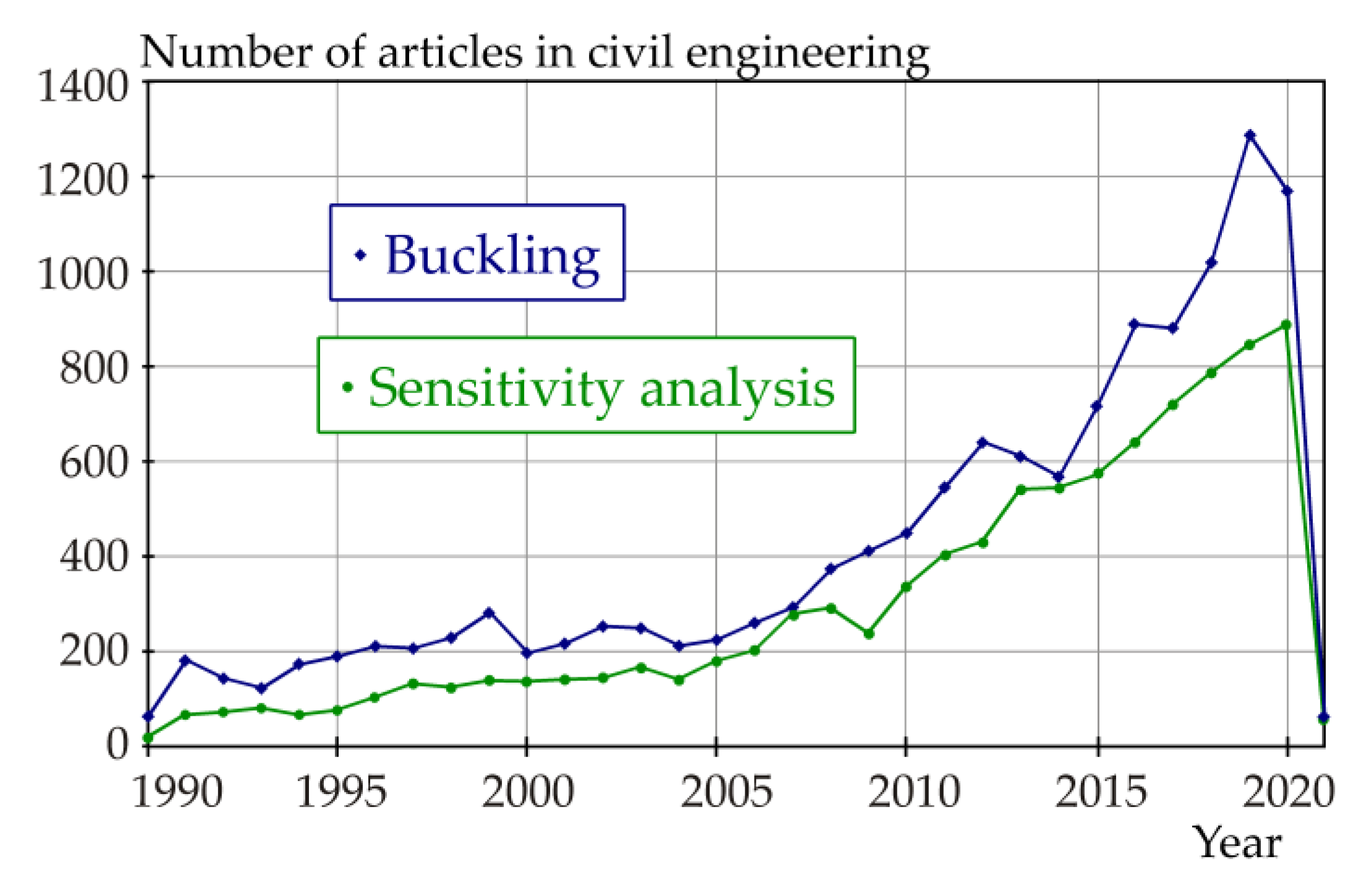
SA is a multidisciplinary science and, therefore, review articles focused purely on SA have a multidisciplinary character [14,15,16,17,18,19]. Only approximately 2.5% of all articles on SA are focused on civil engineering. In civil engineering, publications related to SA have a growing trend, but are not as progressive as traditional engineering topics, such as buckling; see Figure 1.
In civil engineering, SA is focused on the stability of steel frames [20], deflection of concrete beams with correlated inputs [21], multiple-criteria decision-making (MCDM) [22], structural response to stochastic dynamic loads [23], rheological properties of asphalt [24], thermal performance of facades [25], strength of reinforced concrete beams [26], use of machines during the construction of tunnels [27], stress-based topology of structural frames [28], seismic response of steel plate shear walls [29], deformation of retaining walls [30], multiple-attribute decision making (MADM) [31], efficiency of the operations of transportation companies [32], unbalanced bidding prices in construction projects [33], shear buckling strength [34], reliability index β of steel girders [35], system reliability [36], seismic response and fragility of transmission toners [37], shear strength of corrugated web panels [38], inelastic response of conical shells [39], fatigue limit state [40], corrosion depth [41], building-specific seismic loss [42], vibration response of train–bridge coupled systems [43], shear strength of reinforced concrete beam–column joints [44], forecasts of groundwater levels [45], equivalent rock strength [46], vertical displacement and maximum axial force of piles [47], regional-scale subsurface flow [48], ultimate limit state of cross-beam structures [49], serviceability limit state of structures [50], deflection of steel frames [51], stability of observatory central detectors [52], bearing deformation and pylon ductility of bridges [53], load-carrying capacity of masonry arch bridges [54], free torsional vibration frequencies of thin-walled beams [55], stress and displacement of pipelines [56], fatigue dynamic reliability of structural members [57], deflection of roof truss structures [58], etc. Studies are performed using very different SA methods, which are not always chosen solely for purpose, but are subject to different paradigms that define what and how it should be investigated. Many studies apply only one type of SA, although more than one suitable SA method can be used. Some of the applied methods are traditional, e.g., applications of derivations [25,28], applications of Sobol SA [42,46] or application of the Borgonovo method [30], but highly specific and original SA methods [23,54], which are difficult or even impossible to compare with conventional methods [1], are also being developed.
In civil engineering, SA objectives are usually focused on the optimization of the properties of structures, design characteristics of structures or processes associated with construction activities. One of the important features of any structure is its reliability.
1.2. Reliability-Oriented Sensitivity Analysis
In civil engineering, structural reliability is assessed using the well-developed concept of limit states [59,60], which clearly defines the design quantiles of resistance and the effect of load action. Regarding the ultimate limit state, a load-bearing structure is considered reliable if the high quantile of load action is smaller than the low quantile of resistance [61].
A comparative study [61] showed large differences between four reliability-oriented sensitivity analyses (ROSA) and additional four SA used in reliability analysis. The conclusions [61] showed that a common platform that clearly translates the correlation between indices and their information value is absent in ROSA methods.
A reliability-oriented SA concept based on design quantiles was introduced in [62]. SA was performed using the total indices of the design quantiles of resistance and load without having to evaluate the SA of failure probability. This saves the computational costs of numerically demanding models. Mirroring the concept of limit states into the principles of SA brings the results of sensitivity studies closer to the engineering practice, reduces computational costs and expands the possibilities of modelers.
This article builds on [62] by introducing more general quadratic forms of quantile-oriented sensitivity indices, which are compared with quantile-oriented sensitivity indices subordinated to contrasts [63]. Two SAs are compared with the classical Sobol SA in a case study using a non-linear function of the elastic static resistance of a compressed steel structural member. The advantages and disadvantages of all three methods are described and discussed.
2. Quantile-Oriented and Sobol Global Sensitivity Indices
From a black box perspective, any model may be regarded as a function R = g(X), where X is a vector of M uncertain model inputs {X1, X2,... XM}, and R is a one-dimensional model output. The uncertain model inputs are considered as statistically independent random variables. This incurs no loss of generality, because mutual relations are created through the computational model on the path to the output.
Three types of global SA (in short SA) are used: Q indices, K indices and Sobol indices. All three types of SA have the ability to measure sensitivity across the input space (i.e., they are global methods), are capable of dealing with non-linear responses, and can quantify the influence of interactions in a non-additive systems. The first two SAs [62,63] are quantile-oriented, the third is the classical Sobol SA [2,3]. Both quantile-oriented SAs can study structural reliability, the assessment of which is based on limit states and design quantiles. The reason for including Sobol SA is its orientation on variance, which is an important, but not the only, part of reliability analysis.
2.1. Linear Form of Quantile-Oriented Sensitivity Indices—Contrast Q Indices
Sensitivity indices subordinated to contrasts associated with quantiles [63] (in short, Contrast Q indices) are based on linear contrast functions. The contrast function ψ associated with the α-quantile of output R can be expressed using parameter θ as
where R is a scalar. Equation (16) attains its minimum if the argument θ has a value of α-quantile of R, see Equation (2)
where θ* is the α-quantile of R. The minimum of Equation (1) can be expressed using θ* as
where l is the absolute difference (distance) between the mean value of the population below the α-quantile θ* and mean value of the population above the α-quantile θ*. Let l be the quantile deviation. The quantile deviation l is the difference between superquantile E(R|R ≥ θ*) and subquantile E(R|R < θ*)
where l = l1 + l2. l1 is the mean absolute deviation from θ* below θ*, l2 is the mean absolute deviation from θ* above the quantile θ* (in short quantile deviation l), and f(r) is the probability density function (pdf) of the model output.
The introduction of superquantile and subquantile in Equation (4) introduces quantile deviation l as a new quantile sensitivity measure.
It can be noted that superquantiles are fundamental building blocks for estimates of risk in finance [64] and engineering [65]. In finance, the superquantile has various names, such as expected tail loss [66], conditional value-at-risk (CVaR) [67,68,69,70] or tail value-at-risk [71], average value at risk [72], expected shortfall [73,74]. Subquantile is not such a widespread concept.
In the context of SA, l was first introduced as a new sensitivity measure in [62]. A property of the quantile deviation l is that it is expressed in the same unit as the data. The quantile deviation l is a robust statistic, which, compared with the standard deviation, is more resilient to outliers in a dataset. This is due to the fact that in the case of standard deviation, i.e., the square root of variance, the distances from the mean are squared, so that large deviations are weighted more and can, therefore, be strongly influenced by outliers. Regarding quantile deviation l, the deviations of a small number of outliers are inconsequential.
With regard to random sampling, the quantile deviation l of a finite observation of size N with values rj can be estimated as
where N1 is the total number of observations below the α-quantile, N2 = N – N1 is the total number of observations above the α-quantile, where α-quantile θ* can be estimated so that α·N observations are smaller than θ* and (1-α)·N observations are greater than θ*.
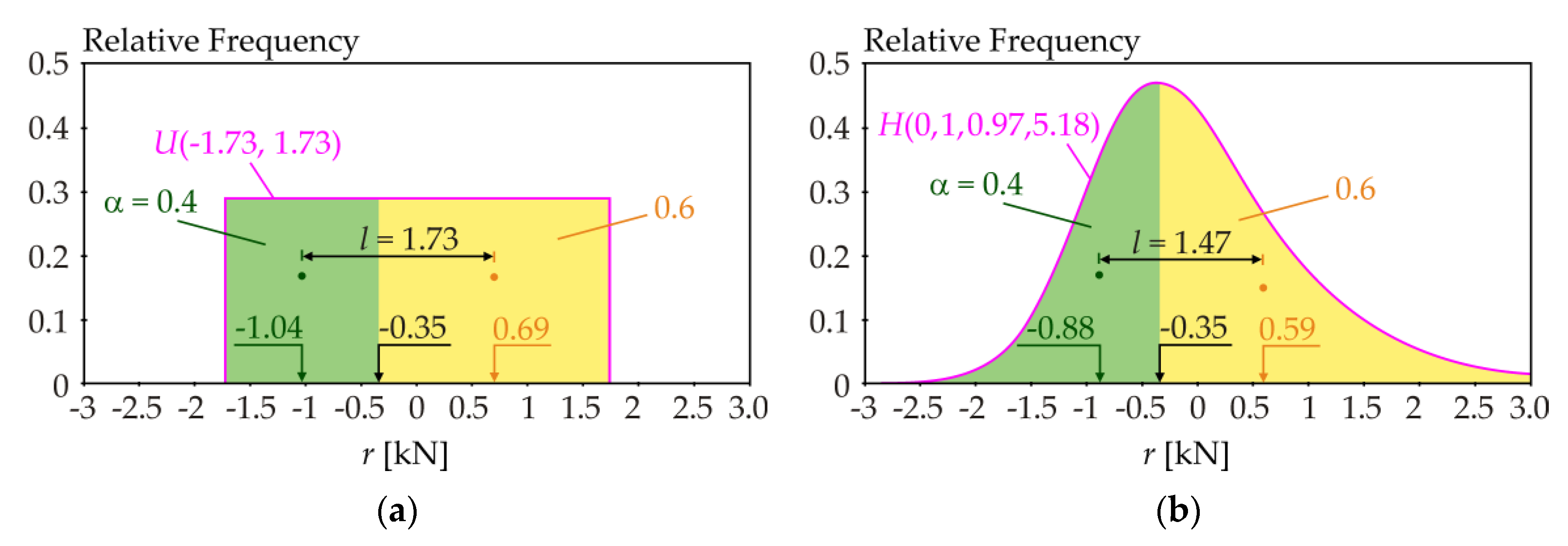
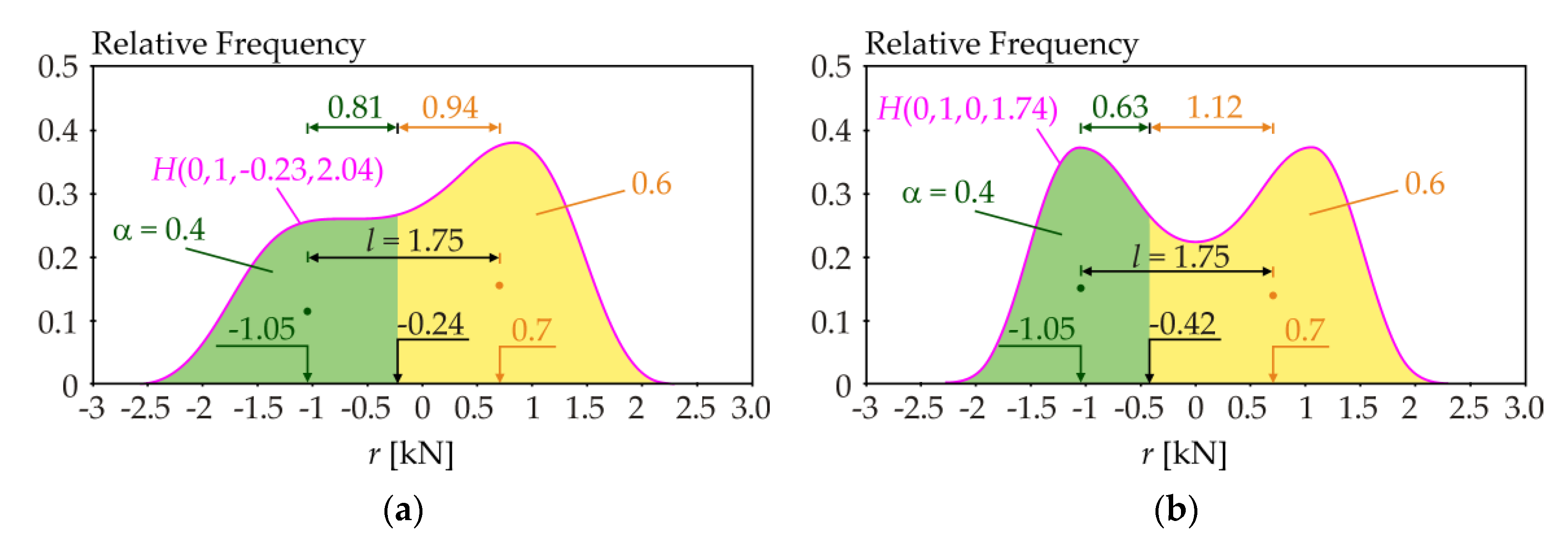
Figure 2 and Figure 3 depict examples of symmetric and asymmetric probability density functions (pdfs), where the value of l is expressed as the distance between the centres of gravity of the green and yellow areas. All probability density functions (pdfs) have mean value μR = 0 and standard deviation σR = 1. Figure 2a depicts the Uniform probability density function (pdf). Figure 2b and Figure 3a,b depict a four-parameter Hermite pdf, where the third and fourth parameters are skewness and kurtosis.
By modifying Equation (3), quantile deviation l can be computed using the probability density function according to Equation (6)
where the value of α·(1 − α) is constant. The first-order contrast Qi index defined in [63] has a form that can be rewritten using the quantile deviation l as Equation (7)
where the mean value E(·) is considered over all likely values of Xi. The new form of the contrast index Qi is
In a general model, fixing Xi can change all the statistical characteristics of output R. Only the changes in l caused by changes in Xi are important for the value of index Qi; see Equation (8). What statistical characteristics does l depend on? The quantile deviation l is not dependent on μR. Changes in l would hypothetically depend only on changes in σR provided that the shape of the pdf does not change (e.g., still Gaussian output in additive model with Gaussian inputs). However, this cannot be generally assumed.
Figure 2 shows an example where changing the shape of the pdf causes a change in l from l = 1.73 to l = 1.47 when μR = 1 and σR = 1 is considered. Analogously, changing the shape of the pdf can change σR, but not l. Figure 3 shows an example where changing the pdf shape does not cause a change in l when μR = 1 and σR = 1 is considered. Therefore, changing the shape of the pdf may or may not affect l. The skewness and kurtosis may or may not affect l. In general, l does not depend on the change of μR itself, but depends on the pdf shape where the influence of moments acts in combinations, which can have a greater or lesser influence on l depending on the specific model type. These questions are examined in more detail in the case study presented in Chapter 5.
The second-order α-quantile contrast index Qij is derived similarly by fixing of pairs Xi, Xj
where E(·) is considered across all Xi and Xj. The third-order sensitivity index Qijk is computed analogously
Statistically independent input random variables are considered. The sum of all indices must be equal to one
The total index QTi can be written as
where the second term in the numerator contains the conditional quantile deviation l evaluated for input random variable Xi and fixed variables (X1, X2,…, Xi–1, Xi+1,…, XM).
Contrast Q indices expressed using the quantile deviation l are the same as the indices based on contrasts defined in [63], but are obtained in a different way. Contrast Q indices can also be written in an asymptotic form [62] (p. 15), which is based on measuring the distance between an α-quantile θ* and the mean value μ of the model output l ≈ ±(θ* − μ), but limited to only large and small quantiles.
The contrast Q indices described in this chapter use quantile deviation l in linear form.
2.2. Quadratic Form of Quantile-Oriented Sensitivity Indices—K Indices
New sensitivity indices focused on quantiles can be obtained using the square of the quantile deviation l. The basic concept of this quadratic form of quantile-oriented sensitivity analysis was introduced in [62] (p. 16). Unlike contrast Q indices, the sensitivity measure is expressed in the same unit as the variance. The decomposition of l2 can be performed in a similar manner to the decomposition of the variance in Sobol sensitivity indices [62]. The asymptotic form of these indices has been denoted as QE indices [62].
The first-order Ki index can be written as
The second-order index Kij is computed similarly with fixing of pairs Xi, Xj
The third-order sensitivity index Kijk is computed analogously
The other higher-order indices are obtained similarly. Statistically independent input random variables are considered. The sum of all indices must be equal to one
The total index KTi can be written as
where the second term in the numerator contains the conditional parameter l2 evaluated for input random variable Xi and fixed variables (X1, X2, …, Xi–1, Xi+1,…, XM). Equations (13)–(17) can be used for all quantiles, i.e., they are not limited to small and large quantiles.
2.3. Sobol Sensitivity Indices—Sobol Indices
Sobol variance-based sensitivity analysis is the most frequently used SA method [2,3]. Sobol SA is based on the decomposition of the variance of the model output. Sobol SA estimates the degree of variance that each parameter contributes to the model output, including interaction effects. The first-order Si index can be written as
where E(·) is considered across all Xi. The total effect index STi, which measures first and higher-order effects (interactions) of variable Xi, is another popular variance-based measure [1]
where the second term in the numerator contains the conditional variance evaluated for input random variable Xi and fixed variables (X1, X2, …, Xi–1, Xi+1, …, XM).
Sobol SA is dependent only on the variance. The similarity of the results of Sobol SA and quantile-oriented SA can be sought in connection with the degree of the influence of the variance on the quantile.
3. Resistance of Steel Member under Compression
Most forms of civil engineering structures are designed using European unified design rules [75]—Eurocodes. The limit state is the structural condition past which it no longer satisfies the pertinent design criteria [76]. Limit state design requires the structure to satisfy two fundamental conditions: the ultimate limit state (strength and stability) and the serviceability limit state (deflection, cracking, vibration).
The aim of the case study presented in this article is to analyse the static resistance (load-carrying capacity) of a slender steel member, which is limited by the strength of the material and stability. The resistance R is a random variable that depends on material and geometrical characteristics, which are generally random variables. A structure is considered to satisfy the ultimate limit state criterion if the random realization of the external load action is less than the low (design) quantile of load-carrying capacity Rd. Standard [59] enables the determination of design value Rd as 0.1 percentile [77,78,79,80,81].
The stochastic model of ultimate limit state of a hot-rolled steel member under longitudinal compression load action F is shown in Figure 4a. Biaxially symmetrical cross section HEA 180 of steel grade S235 is considered; see Figure 4b.
The resistance of the steel structural member shown in Figure 4a was derived in [82] using the equation e = e0/(1 − F/Fcr), where Fcr is Euler’s critical load. Increasing the external load action F increases the compressive stress σx until the yield strength fy is attained in the middle of the span in the lower (extremely compressed) part of the cross-section; see Figure 4a. Hooke’s law with Young’s modulus E is considered. The dependence of σx on F is non-linear if e0 > 0, where F < Fcr. The elastic resistance R (unit Newton) is the maximum load action F; a higher value of force F would cause overstressing and structural failure. The resistance R can be computed using the response function [82]
where
where e0 is the amplitude of initial axis curvature, L is the member length, h is the cross-sectional height, b is the cross-sectional width, t1 is the web thickness and t2 is the flange thickness. These variables are used to further compute the following variables: A is cross-sectional area and Iz is second moment of area around axis z.
It can be noted that e0 is the amplitude of pure geometrical imperfection with an idealized shape according to the elastic critical buckling mode [83]. Amplitude e0 is not an equivalent geometrical imperfection [84,85,86], which would replace the influence of other imperfections, such as the residual stress. In Equation (20), the influence of residual stress is neglected.
The member length L is a deterministic parameter. Equation (20) is a non-linear, non-monotonic function for R > 0 that has the typical elastic resistance properties of a compressed member with initial material and geometrical imperfections with the exception of residual stress. Although R is a vector quantity, the direction is still horizontal; see Figure 4a) and only the magnitude is a random variable. Thus, in this article, the resistance R is examined as a scalar model output.
The material and geometrical characteristics of hot-rolled steel beams have been studied experimentally [87,88]. Studies [82,89,90,91] have confirmed that the variance of t1 and h have a minimal influence on R. Therefore, these variables can be considered as deterministic with values t1 = 6 mm and h = 171 mm. The input random variables are listed in Table 1. All random variables are statistically independent of each other.
All random variables have Gauss pdf, but with the condition fy > 0, E > 0, t2 > 0 and b > 0. However, negative realizations of random variables fy, E, t2 and b practically never occur if the LHS method [92,93] is used with no more than tens of millions of runs. Theoretically, if fy → 0 then R → 0 (due to no stress), if E → 0 then R → 0 (due to zero stiffness), if e0 → 0 then R → Fcr or R → fy·A (pure buckling for high L or simple compression for low L), if L → 0 then R → fy·A (simple compression).
4. Results of Sensitivity Analysis
The member length L is a deterministic parameter that changes step-by-step as L = 0.001, 0.424, 0.849, …, 6.366 m. The step value is L0/10, where L0 = 4.244 m is the length of the member with non-dimensional slenderness [94] = 1.0. The common non-dimensional slenderness of a strut in an efficient structural system is around one, but struts usually do not have non-dimensional slenderness higher than two [95]. The slenderness is directly proportional to the length. It is possible, for the presented case study, to write the transformation L =· L0, which makes it easier to understand the lengths.
All three types of SA are based on double-nested-loop algorithms. Estimation of indices was software-based by implementing randomized Latin Hypercube Sampling-based Monte Carlo simulation (LHS) algorithms [92,93], which have been tuned for sensitivity assessments [78,80]. Using LHS runs, the outer loop is repeated 2000 times to estimate the arithmetic mean E(·) of the samples (l, l2 or variance), which are estimated using an inner loop algorithm. The inner loop is repeated 4 million times (4 million LHS runs) to compute statistics (l, l2 or variance) with some random realizations fixed by the outer loop.
The subject of interest for the two quantile-oriented SA is the 0.001-quantile θ* of R. The estimate l quantifies the population distribution around the 0.001-quantile θ*, where 0.001-quantile θ* is estimated as the 4000th smallest value in the set of four million LHS runs ordered from smallest to largest [78,80].
The estimates of the unconditional characteristics in the denominators of the indices are computed using four million runs of the LHS method. Higher-order indices are estimated similarly.
The same set of (pseudo-) random numbers is used in each member length L, hereby ensuring that sampling and numerical errors do not swamp the statistics being sought [96,97].
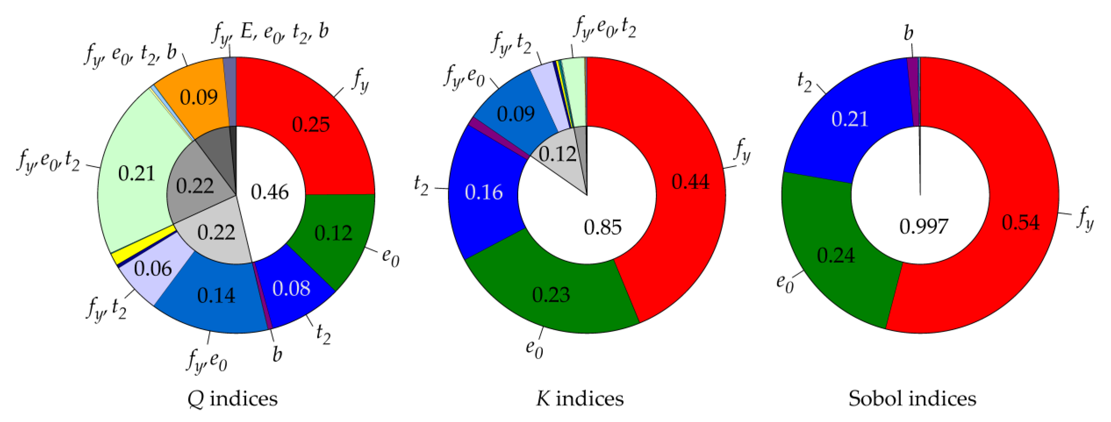
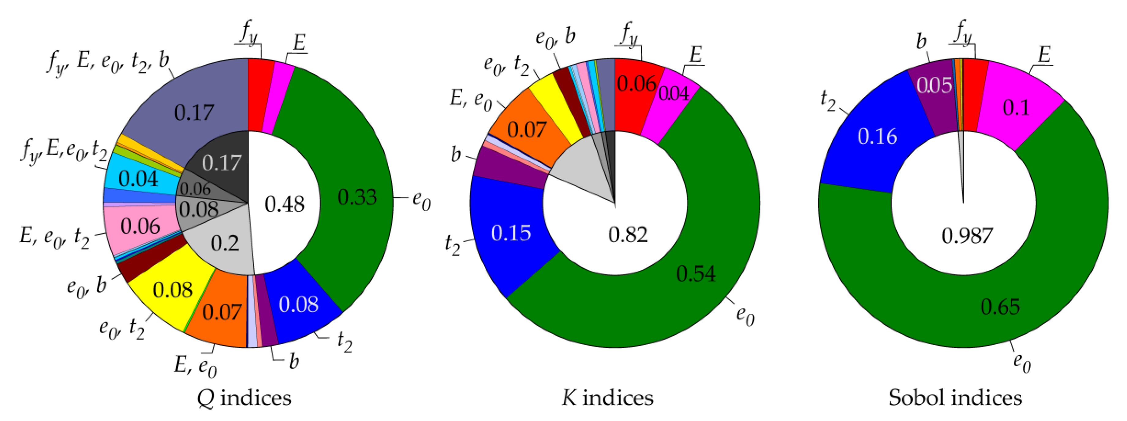
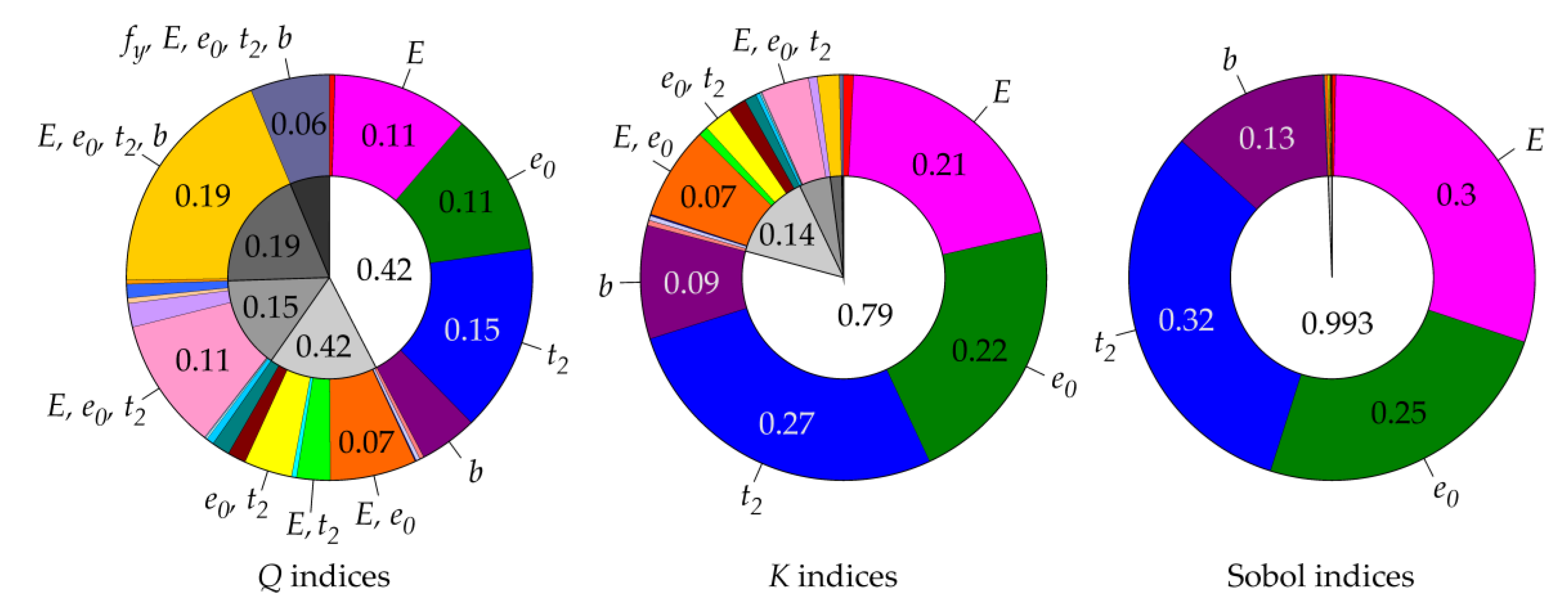
Figure 5, Figure 6, Figure 7 and Figure 8 show contrast Q indices, K indices and Sobol indices for four selected member lengths corresponding to non-dimensional slenderness values = 0, 0.5, 1, 1.5. The outer coloured ring displays 31 sensitivity indices, and the inner white-grey pie chart shows the representation of member lengths of first-order indices (white area of the chart) and higher-order indices (grey areas).
The results in Figure 5, Figure 6, Figure 7 and Figure 8 show that Sobol indices have the largest proportion of first-order sensitivity indices; see the white area in the inner circles in Figure 5, Figure 6, Figure 7 and Figure 8. Small higher-order indices make Sobol first-order indices transparent without the need to evaluate total indices. Unfortunately, Sobol indices are not quantile-oriented.
The new quantile-oriented K indices also have a relatively small proportion of higher-order indices (grey areas in the inner circles), and thus approach Sobol indices with their properties. Q indices have the lowest proportion of first-order sensitivity indices and a high proportion of higher-order indices (interaction effects), which makes the results less comprehensible, and the evaluation of total indices is then necessary.
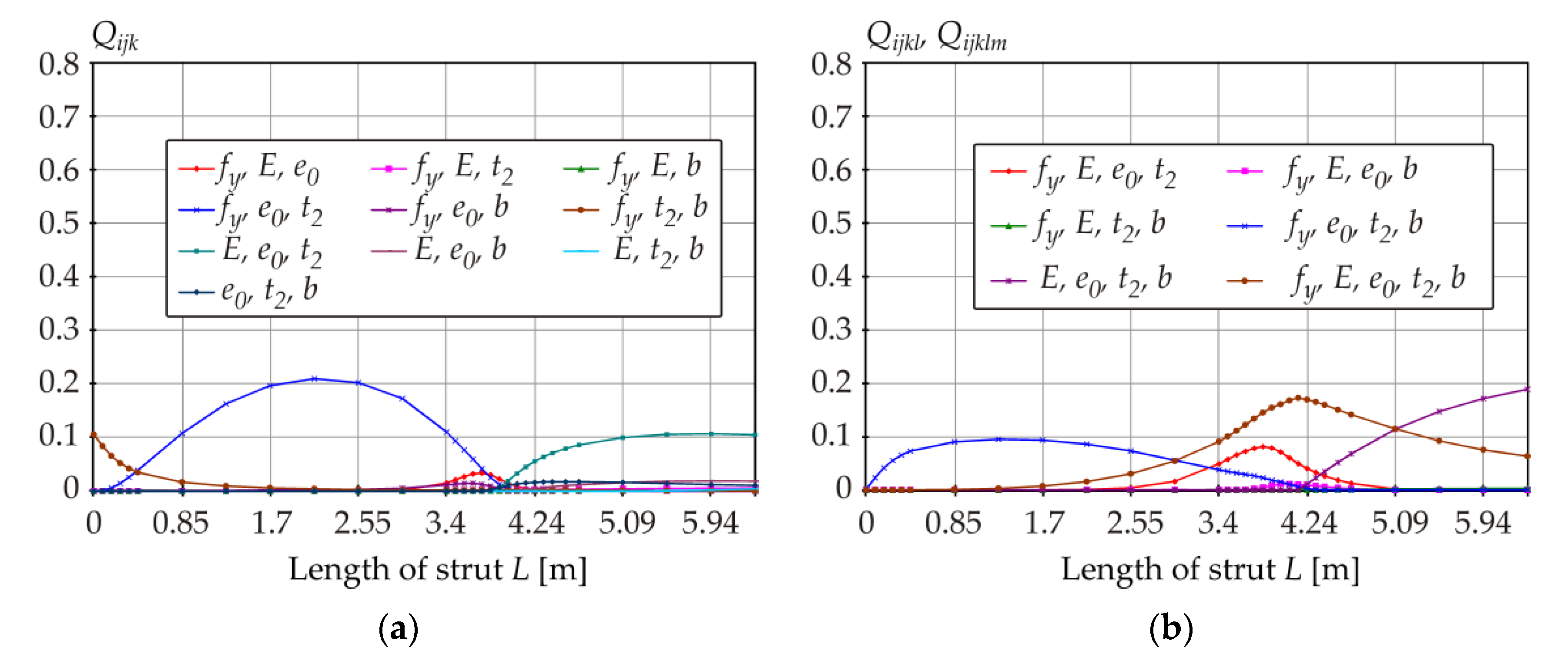
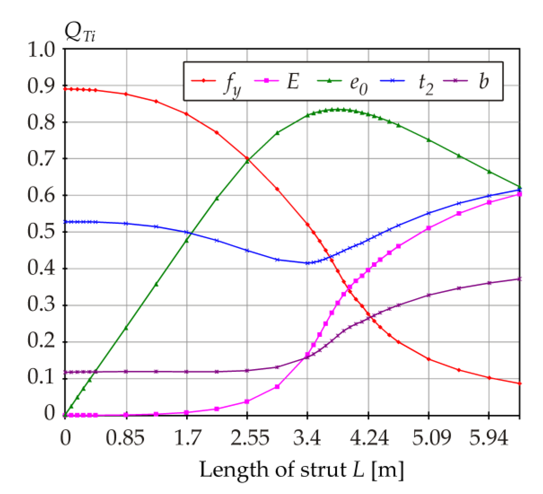
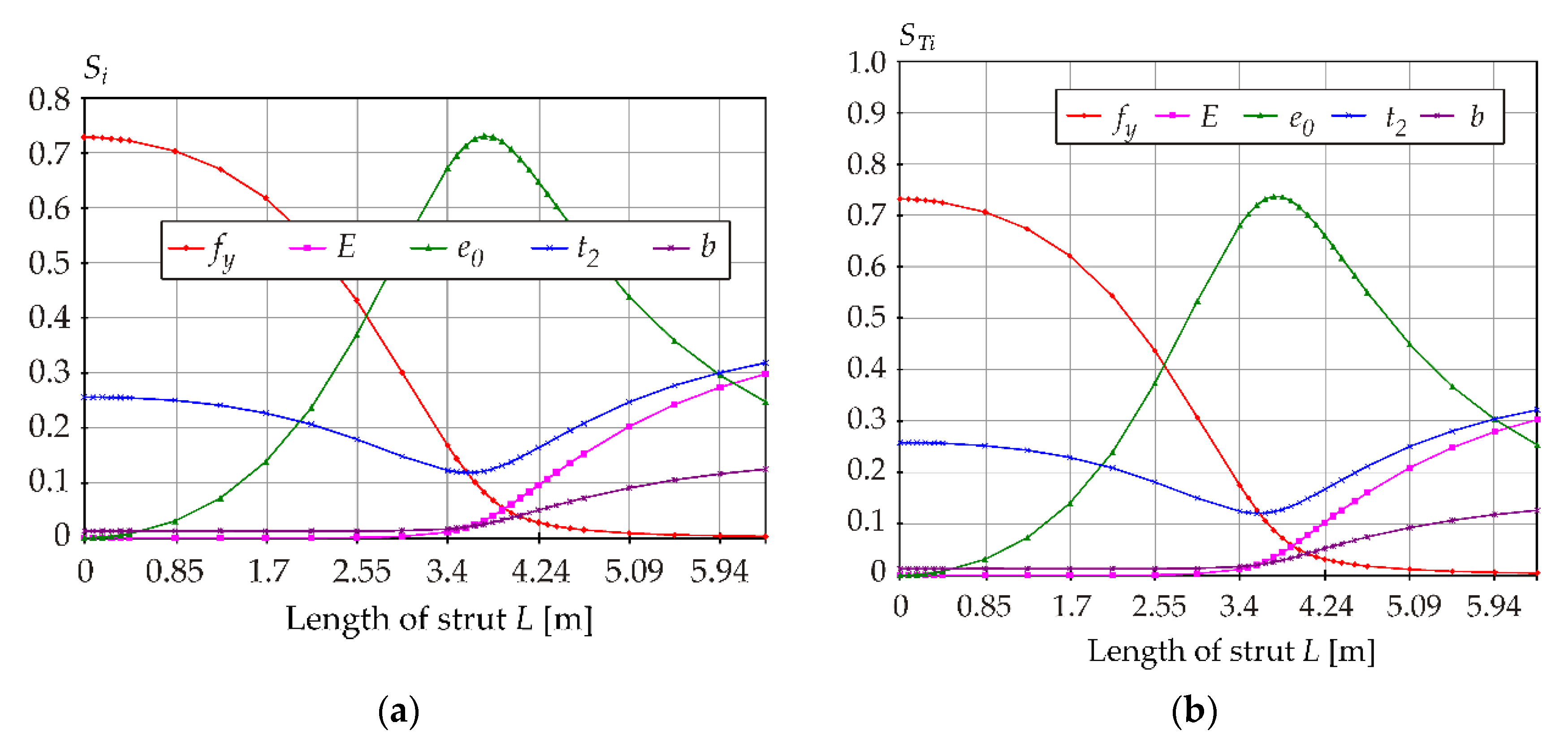
Figure 9 and Figure 10 display the plots of all thirty-one Q indices vs. member length L. A finer step is used in places where the curves change course faster.
As for Q indices, the clear influence of individual variables on the 0.001-quantile of R is evident only after the evaluation of total indices, see Figure 11. The yield strength fy is dominant for low values of L (low slenderness), imperfection e0 is dominant for intermediate lengths L (intermediate slenderness), Young’s modulus and flange thickness gain dominance in the case of long members (high slenderness).
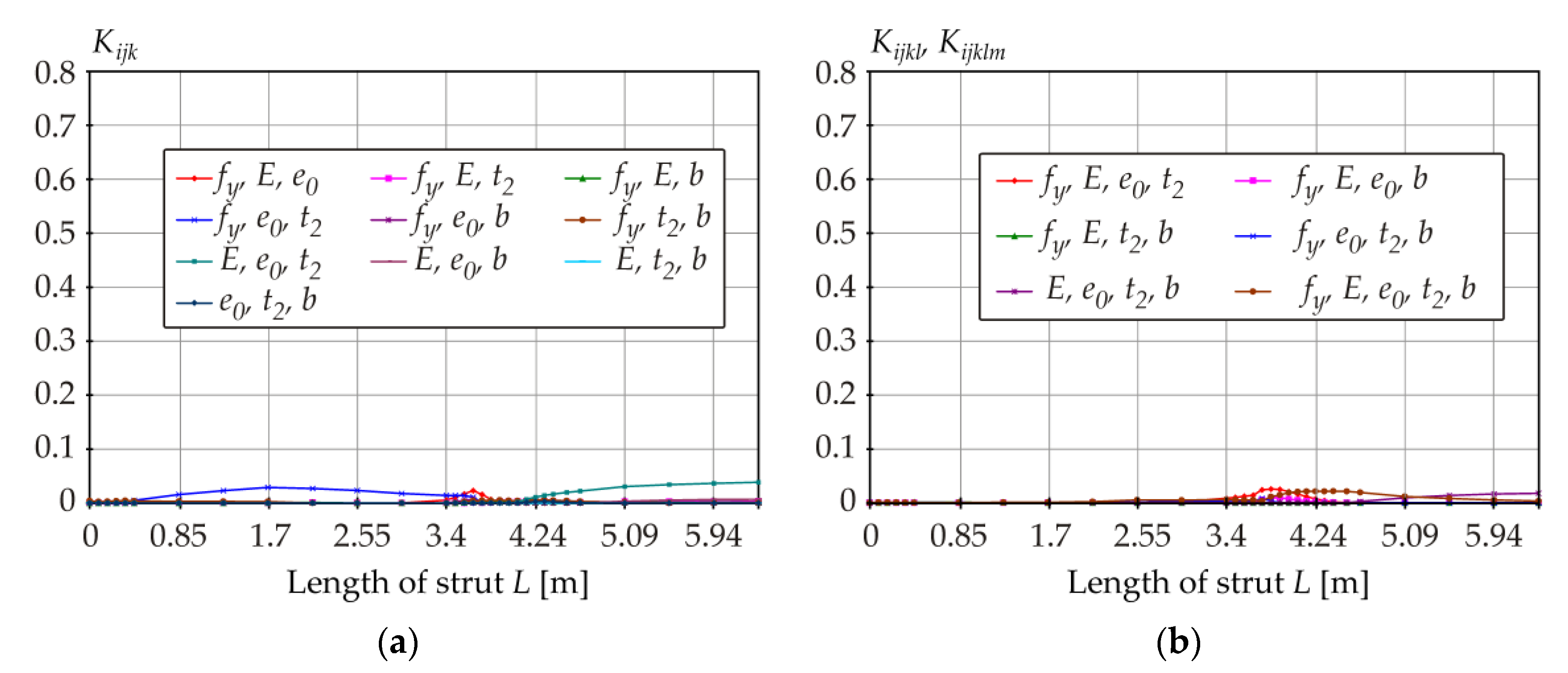
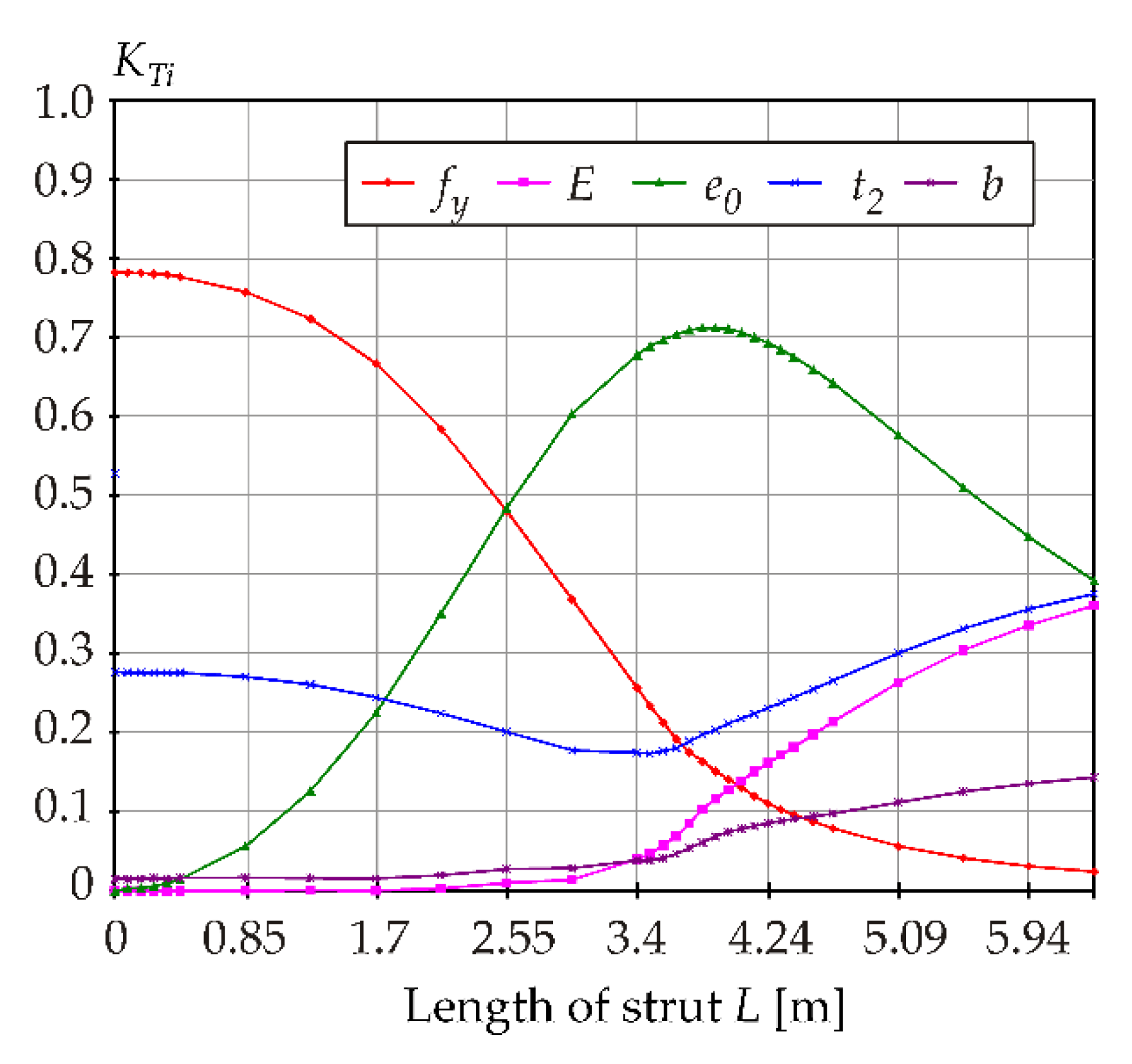
Figure 12 and Figure 13 display the plots of all thirty-one K indices vs. member length, with the proportion of higher-order sensitivity indices being relatively small. The total KT indices shown in Figure 14 provide very similar (but not the same) information as the first-order Ki indices depicted in Figure 12.
Figure 15a shows Sobol first-order sensitivity indices. Sobol higher-order sensitivity indices are not shown because they are practically zero. The total indices shown in Figure 15b provide practically the same information as Sobol first-order sensitivity indices Si.
Examples of percentage differences between first-order indices are as follows. The yield strength has the greatest influence for L = 0 m, with Q1 being 37% smaller than S1, and K1 being 3% smaller than S1. Imperfection e0 has the greatest influence for L ≈ 3.8 m, with Q3 being 46% smaller than S3, and K3 being 16% smaller than S3. Ki indices are closer to Si indices (compared to Qi indices).
The percentage differences between total indices are as follows. The yield strength has the greatest influence for L = 0 m, with QT1 being 22% greater than ST1, and KT1 being 7% greater than ST1. Imperfection e0 has the greatest influence for L ≈ 3.8 m, with QT3 being 13% greater than ST3 and KT3 being 3% smaller than ST3. KTi indices are closer to STi indices (compared to QTi indices).
A comparison of the results of all three types of SA shows that the conclusions are very similar, despite being reached in a different way. The new K indices with their properties approach Sobol indices due to quadratic measures of sensitivity using l2, which behaves similarly to variance .
5. Static Dependencies between l and σR and Other Connections
Quantile-oriented sensitivity indices are based on the quantile deviation l or its square l2 while Sobol sensitivity indices are based on variance . The subject of interest of both quantile-oriented SA is the 0.001-quantile of R.
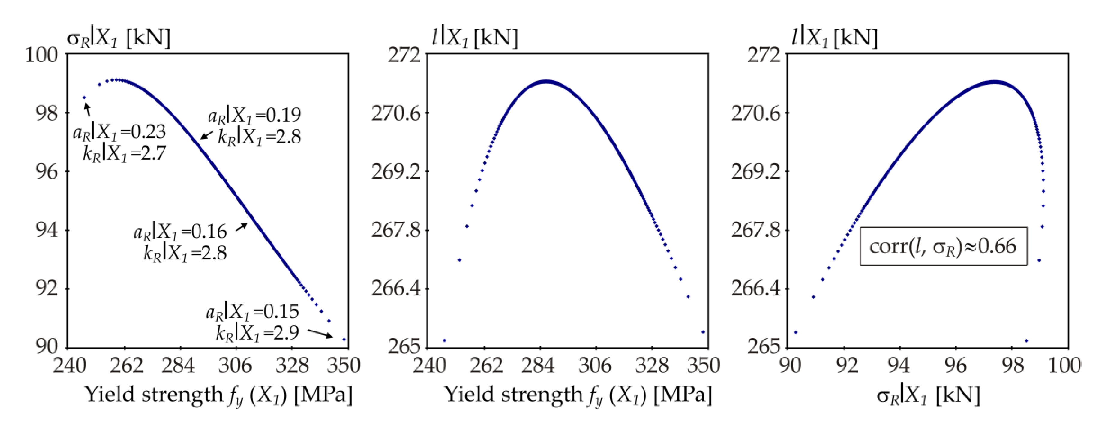
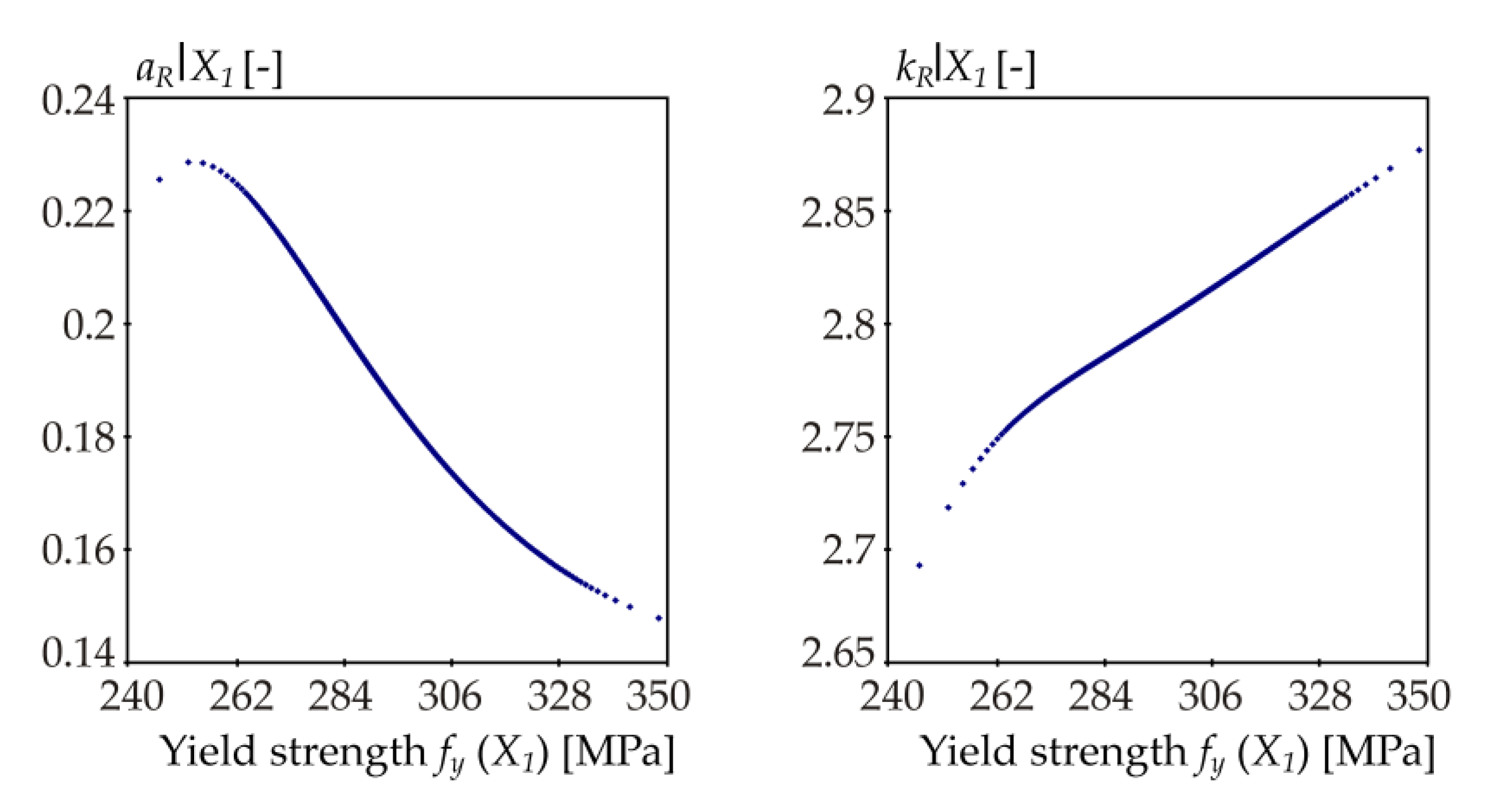
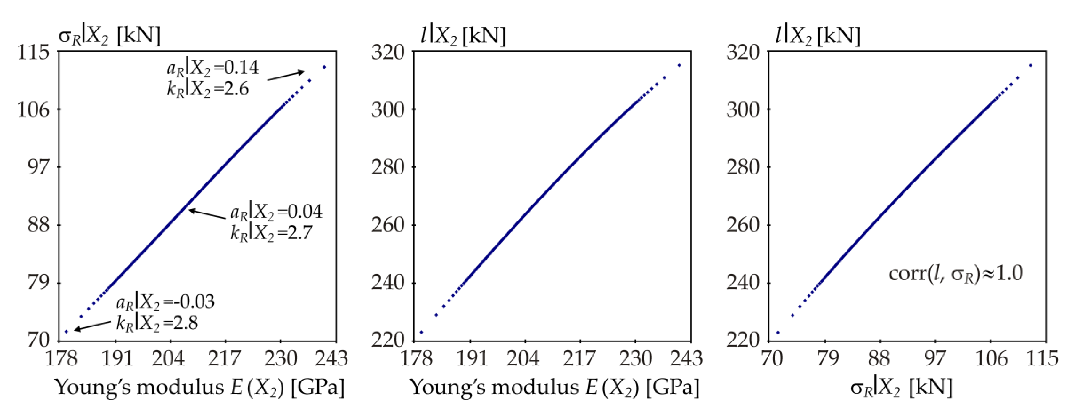
To better understand the essence of the computation of sensitivity indices, screening of statistics l and σR is performed when Xi is fixed. The aim is to identify similarities and differences between l and σR, rather than to accurately quantify sensitivity using Equations (8), (13) and (18). Samples σR|Xi and l|Xi are plotted for 400 LHS runs of Xi, otherwise the solution is the same as in the previous chapter. Skewness aR|Xi and kurtosis kR|Xi are added for selected samples, see Figure 16, Figure 17, Figure 18, Figure 19, Figure 20 and Figure 21.
The samples in Figure 19 are symmetric due to the symmetric shape of the probability distribution (Gauss pdf) of input variable e0 with a mean value of zero. Only the absolute value of this variable is applied in Equation (20). The output R is not monotonically dependent on e0. The practical consequence is that in the case of an even number of LHS runs, it is sufficient to compute the nested loop in Equations (8), (13) and (18) only once for the positive value of random realization e0, because the solution is the same for a negative value. This reduces the computational cost of estimating indices Q3, K3 and S3 by half.
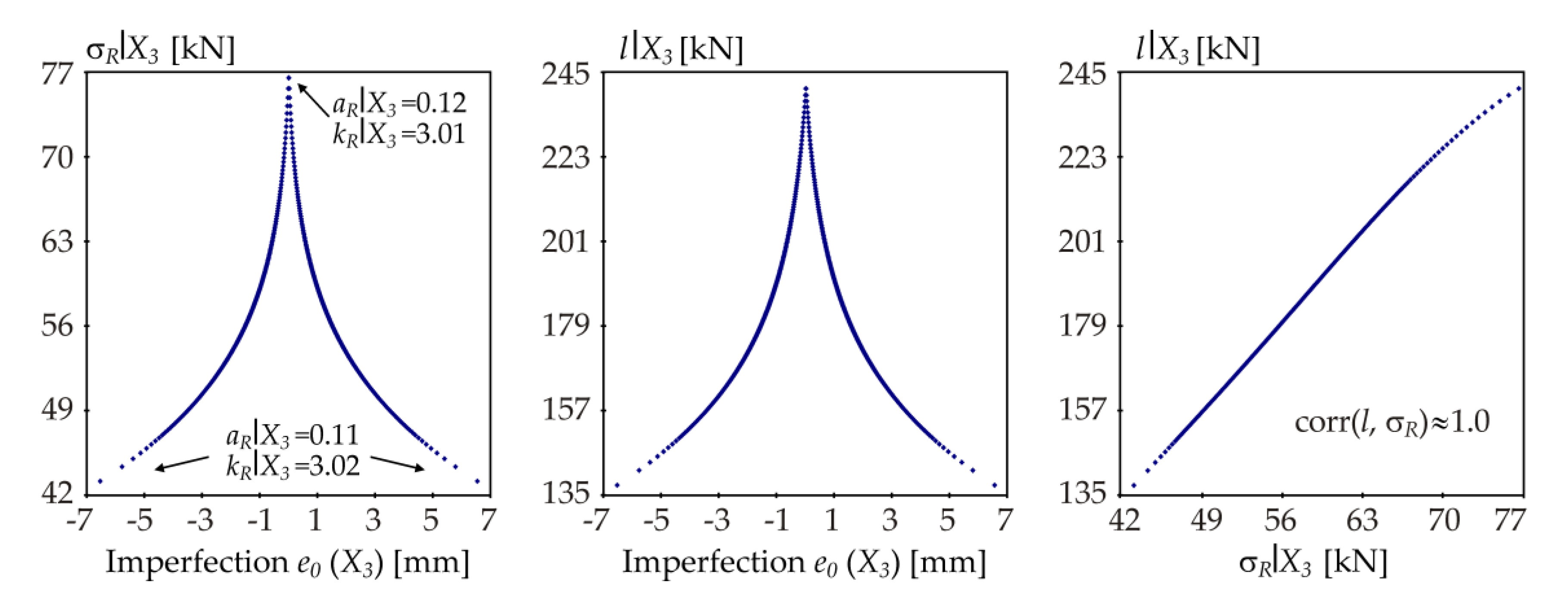
The smaller the estimated σR|Xi, the more fixing of Xi reduces the uncertainty of the output in terms of variance, which measures change around μR. The smaller the estimated l|Xi, the more the fixing of Xi reduces the uncertainty of the output in terms of parameter l, which measures change around θ. Imperfection e0 (X3) has the greatest influence in both cases, see low values on the vertical axes in Figure 19.
In all cases, the dependence l|Xi vs. σR|Xi is approximately linear with the exception of the concave course on the right in Figure 16. Pearson correlation coefficient between 400 samples l|Xi vs. σR|Xi is approximately 0.66. The concave course and lower correlation (compared to other variables) is due to the conflicting influences of σR, aR and kR. By approximating R using the Hermite distribution R~H(μR, σR, aR, kR), the effects of μR, σR, aR and kR on l can be observed separately as follows: change in μR has no influence on l, increasing σR increases l, increasing aR decreases l, increasing kR increases l, assuming small values of changes.
The influence of X1 is interesting. Figure 16, on the left, shows that with increasing X1, σR|X1 has an approximately decreasing plot, with the exception of the beginning on the left. Figure 17 shows that aR|X1 has an approximately decreasing course, kR|X1 has an increasing course. At the beginning on the left, increasing X1 causes an increase in σR|X1, kR|X1 and aR|X1, which, taken together, increases l|X1 due to the dominance of the joint effect of σR|X1, kR|X1 and aR|X1. The region where σR|X1 starts decreasing but l still increases is interesting. Although the standard deviation is an important output characteristic, a change in the input variable can have a stronger influence on the quantile through skewness and kurtosis. At the opposite end (right), increasing X1 causes a decrease in σR|X1, a decrease in aR|X1 and an increase in kR|X1, which together reduces l|X1, because the decreasing sole effect of σR|X1 is dominant. The whole course of l|X1 vs. X1 is shown in Figure 16 in the middle. The example shows the combined effect of standard deviation, skewness and kurtosis on the quantile deviation l, which is the core of the computation of quantile-oriented sensitivity indices Qi and Ki.
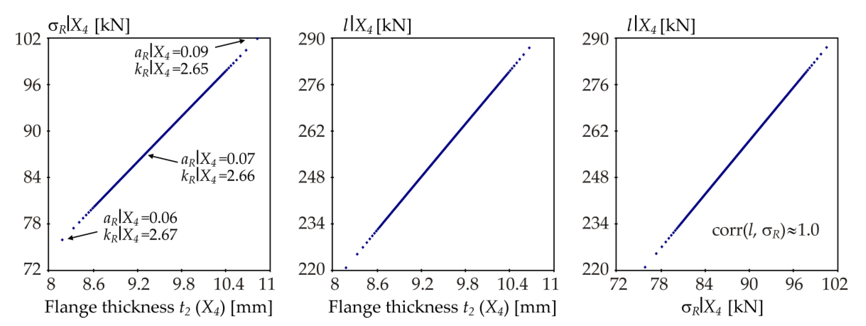
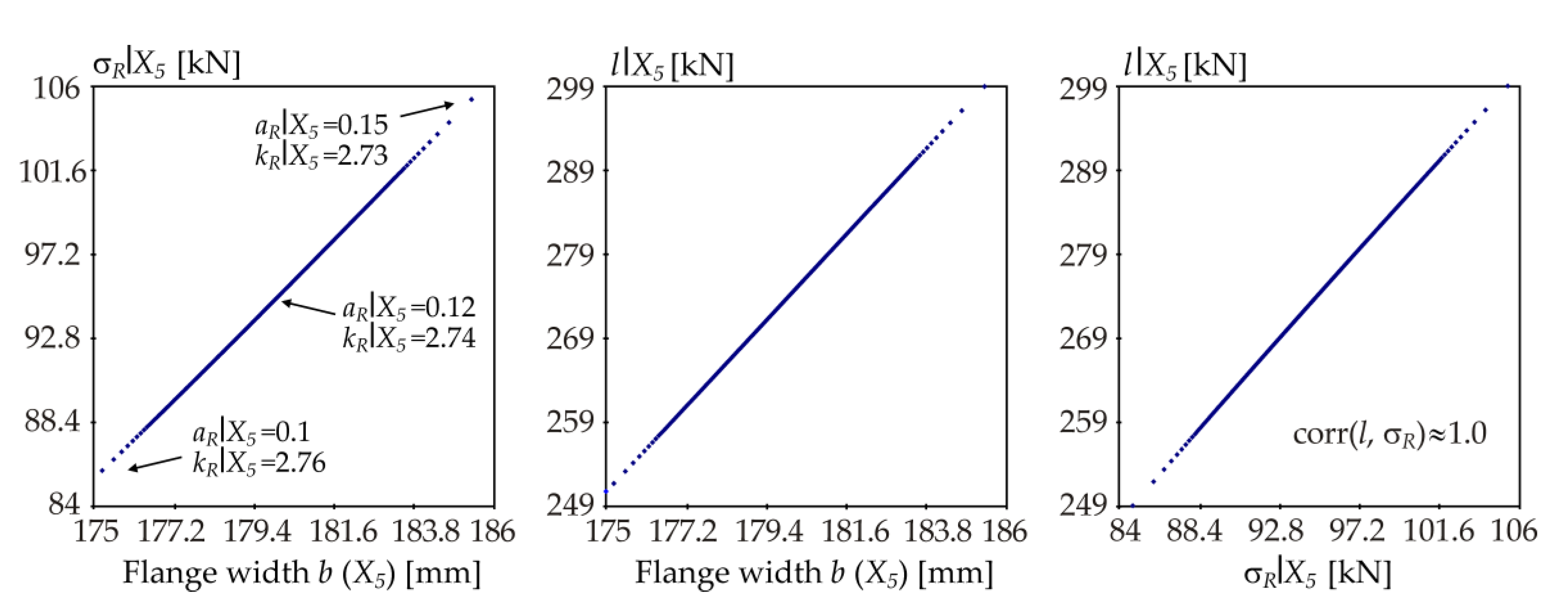
For other variables X2, X3, X4 and X5 the range of σR|Xi is significantly larger than that of σR|X1 (99.1 − 90.3 = 8.8 MPa) and σR|Xi has a crucial influence on l|Xi. Hence, the dependences l|Xi vs. σR|Xi, i = 2, 3, 4, 5 are approximately linear.
6. Discussion
Low quantiles represent a significant part of the analysis of reliability of load-bearing structures. SA of design quantiles can be used wherever reliability can be judged by comparing two statistically independent variables.
Both types of quantile-oriented sensitivity analysis identified a very similar sensitivity order to Sobol SA. Identical identification of probabilistically insignificant variables can serve to reliably decrease the dimension of random design space by introducing non-influential variables as deterministic. On the contrary, the probability distribution of dominant variables should be identified with the greatest possible accuracy.
In all cases, the most important output information is the sensitivity order obtained using total indices. Total indices identify approximately the same sensitivity order for all types of SA; see Figure 11, Figure 14 and Figure 15b. Sobol total indices can be a good proxy of quantile-oriented total indices in cases where changes in the quantile are primarily influenced by changes in the variance and less by the shape of the probability distribution of the output variable R. It can be noted that although the case of strong discrepancy between quantile-oriented indices and Sobol indices has not yet been observed, some atypical (in practice, less real) tasks have not yet been solved, e.g., Sobol SA with strong interaction effects or SA of quantiles close to the mean.
Quantile-oriented contrast Q indices are based on the quantile deviation l, which is the absolute distance of two average values of the population below and above the quantile; see Equations (4)–(6). Quantile deviation l has the same unit and is similar to σR, because it measures the variability of the population around the quantile. Quantile deviation l has good resistance to outlier values around the quantile. When Xi changes deterministically, the quantile deviation l is found to change, but not always monotonically, despite a monotonic variation in the standard deviation σR. The correlation between l and σR may or may not be strong even though a dependence exists; see Figure 16.
By applying the quantile deviation l as a new measure of sensitivity, contrast Q indices defined by Fort [63] can be rewritten in a new form; see Equations (8)–(12). By substituting l with l2, Q indices can be rewritten as the new K indices, which are based on the decomposition of l2, similarly to the way Sobol indices are based on the decomposition of variance; see Equations (13)–(17).
Contrast Q indices have an unpleasantly relatively high proportion of higher-order indices (interaction effects), which makes it difficult to interpret SA results. The new K indices have characteristics close to Sobol indices because they have a smaller proportion of interaction effects than Q indices. Although K and Sobol indices are similar, they are not the same because the key variable l depends not only on the variance but also on the shape of the distribution (variance, skewness, kurtosis).
The comparison of contrast Q indices, K indices and Sobol indices was performed using a non-linear function R, which includes both non-linear and non-monotonic effects of five input variables Xi on the output. In the case study, four input variables Xi, i = 2, 3, 4, 5 have approximately linear dependence l|Xi vs. σR|Xi, where l and σR are computed for fixed Xi while the other X~i are considered as random. However, this does not apply to input variable X1 (yield strength fy), which leads to a non-linear concave dependence l|Xi vs. σR|Xi. The example shows the strong influence of the shape of the distribution (skewness and kurtosis) on the quantile deviation l as one of the causes leading to differences in K indices from Sobol indices.
The findings presented here correlate very well with the results of SA of a beam under bending exposed to lateral-torsional buckling, where contrast Q indices and Sobol indices identified very similar sensitivity rank of input random variables [78,80].
Although other types of quantile-oriented sensitivity indices exist [98,99,100], they are not of a global type with the sum of all indices equal to one, so they were not used in this paper, because mutual comparison would be difficult.
The K indices and Q indices presented here are as computationally demanding as the sensitivity indices derived in [62], but with the advantage that they are not limited to small and large quantiles. For small 0.001-quantile, the estimates of asymptotic QE indices [62] are practically the same as the results published in this article; therefore, the asymptotic form [62] does not provide any immediately apparent application advantage when the Monte Carlo method is applied.
7. Conclusions
Low and high quantiles represent a significant part of the analysis of reliability, not only in the design of building structures. The sensitivity analysis of the resistance R of the steel strut showed significant similarities and differences between both types of quantile-oriented sensitivity analysis (SA) and classical Sobol SA.
The quantile deviation l was defined as the difference between superquantile and subquantile. New global sensitivity measures based on the quantile deviation l of model output were introduced. The quantile deviation l measures the statistical variability around the quantile similarly to how standard deviation measures the statistical variability around the mean value. By using l to the first power, it is possible to rewrite quantile-oriented sensitivity indices subordinated to contrasts (Q indices) in a new form. The obtained results of the presented case study established that Q indices are the least comprehensible because they exhibit the strongest interaction effects between inputs. The results of Sobol SA are clear; however, they are not directly oriented to design quantiles and reliability.
With this motivation in mind, new quantile-oriented sensitivity indices (K indices) are expressed in this paper with sensitivity measure l2 expressed in the same unit as variance, thus approaching Sobol sensitivity indices with their properties. l2 has a significance similar to variance, but around quantile. The unit consistency between K indices and Sobol indices makes K indices attractive in stochastic models, where more parameters (goals) of the probability distribution of the model output need to be analysed. Overall, the new K indices can be considered effective in solving the effect of input random variables on design quantiles.
The case study based on a non-linear and non-monotonic function showed that all three types of SA give very similar conclusions when total indices are evaluated. Although Sobol SA is based on the decomposition of only the variance of the model output, its conclusions are in good agreement with the conclusions of both quantile-oriented SA. The case study showed that the correlation between quantile deviation l and standard deviation σR may or may not be strong. Although l correlates with σR, l is also related to the shape of the probability distribution.
In general, it is always better to prioritize quantile-oriented types of global SA, which measure the statistical variability around a quantile (e.g., quantile deviation l) rather than around a mean value (variance), for quantile-based reliability analysis.
Funding
The work has been supported and prepared within the project namely “Probability oriented global sensitivity measures of structural reliability” of The Czech Science Foundation (GACR, https://gacr.cz/) no. 20-01734S, Czechia.
Institutional Review Board Statement
Not applicable.
Informed Consent Statement
Not applicable.
Data Availability Statement
Not applicable.
Conflicts of Interest
The author declares no conflict of interest.
References
- Saltelli, A.; Ratto, M.; Andres, T.; Campolongo, F.; Cariboni, J.; Gatelli, D.; Saisana, M.; Tarantola, S. Global Sensitivity Analysis: The Primer; John Wiley & Sons: West Sussex, UK, 2008. [Google Scholar]
- Sobol, I.M. Sensitivity Estimates for Non-linear Mathematical Models. Math. Model. Comput. Exp. 1993, 1, 407–414. [Google Scholar]
- Sobol, I.M. Global Sensitivity Indices for Nonlinear Mathematical Models and Their Monte Carlo Estimates. Math. Comput. Simul. 2001, 55, 271–280. [Google Scholar] [CrossRef]
- Gödel, M.; Fischer, R.; Köster, G. Sensitivity Analysis for Microscopic Crowd Simulation. Algorithms 2020, 13, 162. [Google Scholar] [CrossRef]
- Gao, P.; Li, J.; Zhai, J.; Tao, Y.; Han, Q. A Novel Optimization Layout Method for Clamps in a Pipeline System. Appl. Sci. 2020, 10, 390. [Google Scholar] [CrossRef] [Green Version]
- Gatel, L.; Lauvernet, C.; Carluer, N.; Weill, S.; Paniconi, C. Sobol Global Sensitivity Analysis of a Coupled Surface/Subsurface Water Flow and Reactive Solute Transfer Model on a Real Hillslope. Water 2020, 12, 121. [Google Scholar] [CrossRef] [Green Version]
- Prikaziuk, E.; van der Tol, C. Global Sensitivity Analysis of the SCOPE Model in Sentinel-3 Bands: Thermal Domain Focus. Remote Sens. 2019, 11, 2424. [Google Scholar] [CrossRef] [Green Version]
- Dimov, I.; Georgieva, R. Monte Carlo Algorithms for Evaluating Sobol’ Sensitivity Indices. Math. Comput. Simul. 2010, 81, 506–514. [Google Scholar] [CrossRef]
- Gamannossi, A.; Amerini, A.; Mazzei, L.; Bacci, T.; Poggiali, M.; Andreini, A. Uncertainty Quantification of Film Cooling Performance of an Industrial Gas Turbine Vane. Entropy 2020, 22, 16. [Google Scholar] [CrossRef] [PubMed] [Green Version]
- Xu, N.; Luo, J.; Zuo, J.; Hu, X.; Dong, J.; Wu, T.; Wu, S.; Liu, H. Accurate Suitability Evaluation of Large-Scale Roof Greening Based on RS and GIS Methods. Sustainability 2020, 12, 4375. [Google Scholar] [CrossRef]
- Islam, A.B.M.; Karadoğan, E. Analysis of One-Dimensional Ivshin–Pence Shape Memory Alloy Constitutive Model for Sensitivity and Uncertainty. Materials 2020, 13, 1482. [Google Scholar] [CrossRef] [PubMed] [Green Version]
- Mattei, A.; Goblet, P.; Barbecot, F.; Guillon, S.; Coquet, Y.; Wang, S. Can Soil Hydraulic Parameters be Estimated from the Stable Isotope Composition of Pore Water from a Single Soil Profile? Water 2020, 12, 393. [Google Scholar] [CrossRef] [Green Version]
- Akbari, S.; Mahmood, S.M.; Ghaedi, H.; Al-Hajri, S. A New Empirical Model for Viscosity of Sulfonated Polyacrylamide Polymers. Polymers 2019, 11, 1046. [Google Scholar] [CrossRef] [PubMed] [Green Version]
- Koo, H.; Iwanaga, T.; Croke, B.F.W.; Jakeman, A.J.; Yang, J.; Wang, H.-H.; Sun, X.; Lü, G.; Li, X.; Yue, T.; et al. Position Paper: Sensitivity Analysis of Spatially Distributed Environmental Models- a Pragmatic Framework for the Exploration of Uncertainty Sources. Environ. Model. Softw. 2020, 134, 104857. [Google Scholar] [CrossRef]
- Douglas-Smith, D.; Iwanaga, T.; Croke, B.F.W.; Jakeman, A.J. Title. Certain Trends in Uncertainty and Sensitivity Analysis: An Overview of Software Tools and Techniques. Environ. Model. Softw. 2020, 124, 104588. [Google Scholar] [CrossRef]
- Norton, J. An Introduction to Sensitivity Assessment of Simulation Models. Environ. Model. Softw. 2015, 69, 166–174. [Google Scholar] [CrossRef]
- Wei, P.; Lu, Z.; Song, J. Variable Importance Analysis: A Comprehensive Review. Reliab. Eng. Syst. Saf. 2015, 142, 399–432. [Google Scholar] [CrossRef]
- Razavi, S.; Gupta, H.V. What Do We Mean by Sensitivity Analysis? The Need for Comprehensive Characterization of “Global” Sensitivity in Earth and Environmental Systems Models. Water Resour. Res. 2015, 51, 3070–3092. [Google Scholar] [CrossRef]
- Borgonovo, E.; Plischke, E. Sensitivity Analysis: A Review of Recent Advances. Eur. J. Oper. Res. 2016, 248, 869–887. [Google Scholar] [CrossRef]
- Ma, T.; Xu, L. Story-Based Stability of Multistory Steel Semibraced and Unbraced Frames with Semirigid Connections. J. Struct. Eng. 2021, 147, 04020304. [Google Scholar] [CrossRef]
- Pan, L.; Novák, L.; Lehký, D.; Novák, D.; Cao, M. Neural Network Ensemble-based Sensitivity Analysis in Structural Engineering: Comparison of Selected Methods and the Influence of Statistical Correlation. Comput. Struct. 2021, 242, 106376. [Google Scholar] [CrossRef]
- Antucheviciene, J.; Kala, Z.; Marzouk, M.; Vaidogas, E.R. Solving Civil Engineering Problems by Means of Fuzzy and Stochastic MCDM Methods: Current State and Future Research. Math. Probl. Eng. 2015, 2015, 362579. [Google Scholar] [CrossRef] [Green Version]
- Su, C.; Xian, J.; Huang, H. An Iterative Equivalent Linearization Approach for Stochastic Sensitivity Analysis of Hysteretic Systems Under Seismic Excitations Based on Explicit Time-domain Method. Comput. Struct. 2021, 242, 106396. [Google Scholar] [CrossRef]
- Bi, Y.; Wu, S.; Pei, J.; Wen, Y.; Li, R. Correlation Analysis Between Aging Behavior and Rheological Indices of Asphalt Binder. Constr. Build. Mater. 2020, 264, 120176. [Google Scholar] [CrossRef]
- Gelesz, A.; Catto Lucchino, E.; Goia, F.; Serra, V.; Reith, A. Characteristics That Matter in a Climate Facade: A Sensitivity Analysis with Building Energy Simulation Tools. Energy Build. 2020, 229, 110467. [Google Scholar] [CrossRef]
- Naderpour, H.; Haji, M.; Mirrashid, M. Shear Capacity Estimation of FRP-reinforced Concrete Beams Using Computational Intelligence. Structures 2020, 28, 321–328. [Google Scholar] [CrossRef]
- Khetwal, A.; Rostami, J.; Nelson, P.P. Investigating the Impact of TBM Downtimes on Utilization Factor Based on Sensitivity Analysis. Tunn. Undergr. Space Technol. 2020, 106, 103586. [Google Scholar] [CrossRef]
- Changizi, N.; Warn, G.P. Stochastic Stress-based Topology Optimization of Structural Frames Based upon the Second Deviatoric Stress Invariant. Eng. Struct. 2020, 224, 111186. [Google Scholar] [CrossRef]
- Farahbakhshtooli, A.; Bhowmick, A.K. Seismic Collapse Assessment of Stiffened Steel Plate Shear Walls using FEMA P695 Methodology. Eng. Struct. 2019, 200, 109714. [Google Scholar] [CrossRef]
- He, L.; Liu, Y.; Bi, S.; Wang, L.; Broggi, M.; Beer, M. Estimation of Failure Probability in Braced Excavation using Bayesian Networks with Integrated Model Updating. Undergr. Space 2020, 5, 315–323. [Google Scholar] [CrossRef]
- Zolfani, S.H.; Yazdani, M.; Zavadskas, E.K.; Hasheminasab, H. Prospective Madm and Sensitivity Analysis of the Experts Based on Causal Layered Analysis (CLA). Econ. Manag. 2020, 23, 208–223. [Google Scholar]
- Radović, D.; Stević, Ž.; Pamučar, D.; Zavadskas, E.K.; Badi, I.; Antuchevičiene, J.; Turskis, Z. Measuring Performance in Transportation Companies in Developing Countries: A Novel Rough ARAS Model. Symmetry 2018, 10, 434. [Google Scholar] [CrossRef] [Green Version]
- Su, L.; Wang, T.; Li, H.; Chao, Y.; Wang, L. Multi-criteria Decision Making for Identification of Unbalanced Bidding. J. Civ. Eng. Manag. 2020, 26, 43–52. [Google Scholar] [CrossRef]
- Fortan, M.; Ferraz, G.; Lauwens, K.; Molkens, T.; Rossi, B. Shear Buckling of Stainless Steel Plate Girders with Non-rigid end Posts. J. Constr. Steel Res. 2020, 172, 106211. [Google Scholar] [CrossRef]
- Leblouba, M.; Tabsh, S.W.; Barakat, S. Reliability-based Design of Corrugated web Steel Girders in Shear as per AASHTO LRFD. J. Constr. Steel Res 2020, 169, 106013. [Google Scholar] [CrossRef]
- Rykov, V.; Kozyrev, D. On the Reliability Function of a Double Redundant System with General Repair Time Distribution. Appl. Stoch. Models Bus. Ind. 2019, 35, 191–197. [Google Scholar] [CrossRef]
- Pan, H.; Tian, L.; Fu, X.; Li, H. Sensitivities of the Seismic Response and Fragility Estimate of a Transmission Tower to Structural and Ground Motion Uncertainties. J. Constr. Steel Res. 2020, 167, 105941. [Google Scholar] [CrossRef]
- Leblouba, M.; Barakat, S.; Al-Saadon, Z. Shear Behavior of Corrugated Web Panels and Sensitivity Analysis. J. Constr. Steel Res. 2018, 151, 94–107. [Google Scholar] [CrossRef]
- Lellep, J.; Puman, E. Plastic response of conical shells with stiffeners to blast loading. Acta Comment. Univ. Tartu. Math. 2020, 24, 5–18. [Google Scholar] [CrossRef]
- Kala, Z. Estimating probability of fatigue failure of steel structures. Acta Comment. Univ. Tartu. Math. 2019, 23, 245–254. [Google Scholar] [CrossRef]
- Strieška, M.; Koteš, P. Sensitivity of Dose-response Function for Carbon Steel under Various Conditions in Slovakia. Transp. Res. Procedia 2019, 40, 912–919. [Google Scholar] [CrossRef]
- Cremen, G.; Baker, J.W. Variance-based Sensitivity Analyses and Uncertainty Quantification for FEMA P-58 Consequence Predictions. Earthq. Eng. Struct. Dyn. 2020, in press. [Google Scholar] [CrossRef]
- Liu, X.; Jiang, L.; Lai, Z.; Xiang, P.; Chen, Y. Sensitivity and Dynamic Analysis of Train-bridge Coupled System with Multiple Random Factors. Eng. Struct. 2020, 221, 111083. [Google Scholar] [CrossRef]
- Feng, D.-C.; Fu, B. Shear Strength of Internal Reinforced Concrete Beam-Column Joints: Intelligent Modeling Approach and Sensitivity Analysis. Adv. Civ. Eng. 2020, 2020, 8850417. [Google Scholar] [CrossRef]
- Amaranto, A.; Pianosi, F.; Solomatine, D.; Corzo, G.; Muñoz-Arriola, F. Sensitivity Analysis of Data-driven Groundwater Forecasts to Hydroclimatic Controls in Irrigated Croplands. J. Hydrol. 2020, 587, 124957. [Google Scholar] [CrossRef]
- Štefaňák, J.; Kala, Z.; Miča, L.; Norkus, A. Global Sensitivity Analysis for Transformation of Hoek-Brown Failure Criterion for Rock Mass. J. Civ. Eng. Manag. 2018, 24, 390–398. [Google Scholar] [CrossRef]
- Shao, D.; Jiang, G.; Zong, C.; Xing, Y.; Zheng, Z.; Lv, S. Global Sensitivity Analysis of Behavior of Energy Pile under Thermo-mechanical Loads. Soils Found. 2021, in press. [Google Scholar] [CrossRef]
- Erdal, D.; Xiao, S.; Nowak, W.; Cirpka, O.A. Sampling Behavioral Model Parameters for Ensemble-based Sensitivity Analysis using Gaussian Process Eemulation and Active Subspaces. Stoch. Environ. Res. Risk Assess. 2020, 34, 1813–1830. [Google Scholar] [CrossRef]
- Yurchenko, V.; Peleshko, I. Searching for Optimal Pre-Stressing of Steel Bar Structures Based on Sensitivity Analysis. Arch. Civ. Eng. 2020, 66, 525–540. [Google Scholar]
- Liu, F.; Wei, P.; Zhou, C.; Yue, Z. Reliability and Reliability Sensitivity Analysis of Structure by Combining Adaptive Linked Importance Sampling and Kriging Reliability Method. Chin. J. Aeronaut. 2020, 33, 1218–1227. [Google Scholar] [CrossRef]
- Javidan, M.M.; Kim, J. Variance-based Global Sensitivity Analysis for Fuzzy Random Structural Systems. Comput. Aided Civ. Infrastruct. Eng. 2019, 34, 602–615. [Google Scholar] [CrossRef]
- Wan, H.-P.; Zheng, Y.; Luo, Y.; Yang, C.; Xu, X. Comprehensive Sensitivity Analysis of Rotational Stability of a Super-deep Underground Spherical Structure Considering Uncertainty. Adv. Struct. Eng. 2021, 24, 65–78. [Google Scholar] [CrossRef]
- Zhong, J.; Wan, H.-P.; Yuan, W.; He, M.; Ren, W.-X. Risk-informed Sensitivity Analysis and Optimization of Seismic Mitigation Strategy using Gaussian Process Surrogate Model. Soil Dyn. Earthq. Eng. 2020, 138, 106284. [Google Scholar] [CrossRef]
- Vokál, M.; Drahorád, M. Sensitivity Analysis of Input Parameters for Load Carrying Capacity of Masonry Arch Bridges. Acta Polytech. 2020, 60, 349–358. [Google Scholar] [CrossRef]
- Szymczak, C.; Kujawa, M. Sensitivity Analysis of Free Torsional Vibration Frequencies of Thin-walled Laminated Beams Under Axial Load. Contin. Mech. Thermodyn. 2020, 32, 1347–1356. [Google Scholar] [CrossRef] [Green Version]
- Yang, K.; Xue, B.; Fang, H.; Du, X.; Li, B.; Chen, J. Mechanical Sensitivity Analysis of Pipe-liner Composite Structure Under Multi-field Coupling. Structures 2021, 29, 484–493. [Google Scholar] [CrossRef]
- Guo, Q.; Liu, Y.; Liu, X.; Chen, B.; Yao, Q. Fatigue Dynamic Reliability and Global Sensitivity Analysis of Double Random Vibration System Based on Kriging Model. Inverse Probl. Sci. Eng. 2020, 28, 1648–1667. [Google Scholar] [CrossRef]
- Song, S.; Wang, L. A Novel Global Sensitivity Measure Based on Probability Weighted Moments. Symmetry 2021, 13, 90. [Google Scholar] [CrossRef]
- European Committee for Standardization (CEN). EN 1990:2002: Eurocode—Basis of Structural Design; European Committee for Standardization: Brussels, Belgium, 2002. [Google Scholar]
- Joint Committee on Structural Safety (JCSS). Probabilistic Model Code. Available online: https://www.jcss-lc.org/ (accessed on 25 January 2021).
- Kala, Z. Sensitivity Analysis in Probabilistic Structural Design: A Comparison of Selected Techniques. Sustainability 2020, 12, 4788. [Google Scholar] [CrossRef]
- Kala, Z. From Probabilistic to Quantile-oriented Sensitivity Analysis: New Indices of Design Quantiles. Symmetry 2020, 12, 1720. [Google Scholar] [CrossRef]
- Fort, J.C.; Klein, T.; Rachdi, N. New Sensitivity Analysis Subordinated to a Contrast. Commun. Stat. Theory Methods 2016, 45, 4349–4364. [Google Scholar] [CrossRef] [Green Version]
- Rockafellar, R.T.; Uryasev, S. Conditional Value-at-risk for General Loss Distributions. J. Bank. Financ. 2002, 26, 1443–1471. [Google Scholar] [CrossRef]
- Tyrrell Rockafellar, R.; Royset, J.O. Engineering Decisions under Risk Averseness. ASCE-ASME J. Risk Uncertain. Eng. Syst. Part A Civ. Eng. 2015, 1, 04015003. [Google Scholar] [CrossRef] [Green Version]
- Airouss, M.; Tahiri, M.; Lahlou, A.; Hassouni, A. Advanced Expected Tail Loss Measurement and Quantification for the Moroccan All Shares Index Portfolio. Mathematics 2018, 6, 38. [Google Scholar] [CrossRef] [Green Version]
- Rockafellar, R.T.; Royset, J.O. Superquantile/CVaR Risk Measures: Second-order Theory. Ann. Oper. Res. 2018, 262, 3–28. [Google Scholar] [CrossRef] [Green Version]
- Mafusalov, A.; Uryasev, S. CVaR (Superquantile) Norm: Stochastic Case. Eur. J. Oper. Res. 2016, 249, 200–208. [Google Scholar] [CrossRef] [Green Version]
- Hunjra, A.I.; Alawi, S.M.; Colombage, S.; Sahito, U.; Hanif, M. Portfolio Construction by Using Different Risk Models: A Comparison among Diverse Economic Scenarios. Risks 2020, 8, 126. [Google Scholar] [CrossRef]
- Bosch-Badia, M.-T.; Montllor-Serrats, J.; Tarrazon-Rodon, M.-A. Risk Analysis through the Half-Normal Distribution. Mathematics 2020, 8, 2080. [Google Scholar] [CrossRef]
- Norton, M.; Khokhlov, V.; Uryasev, S. Calculating CVaR and bPOE for Common Probability Distributions with Application to Portfolio Optimization and Density Estimation. Ann. Oper. Res. 2019, 1–35. [Google Scholar] [CrossRef] [Green Version]
- Kouri, D.P. Spectral Risk Measures: The Risk Quadrangle and Optimal Approximation. Math. Program. 2019, 174, 525–552. [Google Scholar] [CrossRef]
- Golodnikov, A.; Kuzmenko, V.; Uryasev, S. CVaR Regression Based on the Relation between CVaR and Mixed-Quantile Quadrangles. J. Risk Financ. Manag. 2019, 12, 107. [Google Scholar] [CrossRef] [Green Version]
- Jiménez, I.; Mora-Valencia, A.; Ñíguez, T.-M.; Perote, J. Portfolio Risk Assessment under Dynamic (Equi)Correlation and Semi-Nonparametric Estimation: An Application to Cryptocurrencies. Mathematics 2020, 8, 2110. [Google Scholar] [CrossRef]
- Sedlacek, G.; Müller, C. The European Standard Family and its Basis. J. Constr. Steel Res. 2006, 62, 522–548. [Google Scholar] [CrossRef]
- Sedlacek, G.; Stangenberg, H. Design Philosophy of Eurocodes—Background Information. J. Constr. Steel Res. 2000, 54, 173–190. [Google Scholar] [CrossRef]
- Jönsson, J.; Müller, M.S.; Gamst, C.; Valeš, J.; Kala, Z. Investigation of European Flexural and Lateral Torsional Buckling Interaction. J. Constr. Steel Res. 2019, 156, 105–121. [Google Scholar] [CrossRef]
- Kala, Z. Quantile-oriented Global Sensitivity Analysis of Design Resistance. J. Civ. Eng. Manag. 2019, 25, 297–305. [Google Scholar] [CrossRef] [Green Version]
- Kala, Z.; Valeš, J.; Jönsson, L. Random Fields of Initial out of Straightness Leading to Column Buckling. J. Civ. Eng. Manag. 2017, 23, 902–913. [Google Scholar] [CrossRef] [Green Version]
- Kala, Z. Quantile-based Versus Sobol Sensitivity Analysis in Limit State Design. Structures 2020, 28, 2424–2430. [Google Scholar] [CrossRef]
- Kala, Z.; Valeš, J. Sensitivity Assessment and Lateral-torsional Buckling Design of I-beams Using Solid Finite Elements. J. Constr. Steel Res. 2017, 139, 110–122. [Google Scholar] [CrossRef]
- Kala, Z. Sensitivity Assessment of Steel Members Under Compression. Eng. Struct. 2009, 31, 1344–1348. [Google Scholar] [CrossRef]
- Yang, X.; Xiang, Y.; Luo, Y.-F.; Guo, X.-N.; Liu, J. Axial Compression Capacity of Steel Circular Tube with Large Initial Curvature: Column Curve and Application in Structural Assessment. J. Constr. Steel Res. 2021, 177, 106481. [Google Scholar] [CrossRef]
- Mercier, C.; Khelil, A.; Khamisi, A.; Al Mahmoud, F.; Boissiere, R.; Pamies, A. Analysis of the Global and Local Imperfection of Structural Members and Frames. J. Civ. Eng. Manag. 2019, 25, 805–818. [Google Scholar] [CrossRef]
- Agüero, A.; Baláž, I.; Koleková, Y.; Martin, P. Assessment of in-Plane Behavior of Metal Compressed Members with Equivalent Geometrical Imperfection. Appl. Sci. 2020, 10, 8174. [Google Scholar] [CrossRef]
- Agüero, A.; Baláž, I.; Koleková, Y. New Method for Metal Beams Sensitive to Lateral Torsional Buckling with an Equivalent Geometrical UGLI Imperfection. Structures 2021, 29, 1445–1462. [Google Scholar] [CrossRef]
- Melcher, J.; Kala, Z.; Holický, M.; Fajkus, M.; Rozlívka, L. Design Characteristics of Structural Steels Based on Statistical Analysis of Metallurgical Products. J. Constr. Steel Res. 2004, 60, 795–808. [Google Scholar] [CrossRef]
- Kala, Z.; Melcher, J.; Puklický, L. Material and Geometrical Characteristics of Structural Steels Based on Statistical Analysis of Metallurgical Products. J. Civ. Eng. Manag. 2009, 15, 299–307. [Google Scholar] [CrossRef]
- Kala, Z. Global Sensitivity Analysis in Stability Problems of Steel Frame Structures. J. Civ. Eng. Manag. 2016, 22, 417–424. [Google Scholar] [CrossRef]
- Kala, Z. Geometrically Non-linear Finite Element Reliability Analysis of Steel Plane Frames with Initial Imperfections. J. Civ. Eng. Manag. 2012, 18, 81–90. [Google Scholar] [CrossRef]
- Kala, Z. Sensitivity Analysis of Steel Plane Frames with Initial Imperfections. Eng. Struct. 2011, 33, 2342–2349. [Google Scholar] [CrossRef]
- McKey, M.D.; Beckman, R.J.; Conover, W.J. Comparison of the Three Methods for Selecting Values of Input Variables in the Analysis of Output from a Computer Code. Technometrics 1979, 21, 239–245. [Google Scholar]
- Iman, R.C.; Conover, W.J. Small Sample Sensitivity Analysis Techniques for Computer Models with an Application to Risk Assessment. Commun. Stat. Theory Methods 1980, 9, 1749–1842. [Google Scholar] [CrossRef]
- European Committee for Standardization (CEN). EN 1993-1-9. Eurocode3: Design of Steel Structures, Part 1–1: General Rules and Rules for Buildings; European Standards: Brussels, Belgium, 2005. [Google Scholar]
- Galambos, T.V. Guide to Stability Design Criteria for Metal Structures, 5th ed.; Wiley: Hoboken, NJ, USA, 1998; 911p. [Google Scholar]
- Ahammed, M.; Melchers, R.E. Gradient and Parameter Sensitivity Estimation for Systems Evaluated Using Monte Carlo Analysis. Reliab. Eng. Syst. Saf. 2006, 91, 594–601. [Google Scholar] [CrossRef]
- Rubinstein, R.Y. Simulation and the Monte Carlo Method; John Wiley & Sons: New York, NY, USA, 1981. [Google Scholar]
- Volk-Makarewicz, W.M.; Heidergott, B.F. Sensitivity Analysis of Quantiles. AEnorm 2012, 20, 26–31. [Google Scholar]
- Heidergott, B.F.; Volk-Makarewicz, W.M. A Measure-valued Differentiation Approach to Sensitivities of Quantiles. Math. Oper. Res. 2016, 41, 293–317. [Google Scholar] [CrossRef]
- Kucherenko, S.; Song, S.; Wang, L. Quantile Based Global Sensitivity Measures. Reliab. Eng. Syst. Saf. 2019, 185, 35–48253. [Google Scholar] [CrossRef] [Green Version]
- Koteš, P.; Vavruš, M.; Jošt, J.; Prokop, J. Strengthening of Concrete Column by Using the Wrapper Layer of Fibre Reinforced Concrete. Materials 2020, 13, 5432. [Google Scholar] [CrossRef]
- Kmet, S.; Tomko, M.; Soltys, R.; Rovnak, M.; Demjan, I. Complex Failure Analysis of a Cable-roofed Stadium Structure Based on Diagnostics and Tests. Eng. Fail. Anal. 2019, 103, 443–461. [Google Scholar] [CrossRef]
- Norkus, A.; Martinkus, V. Experimental Study on Bearing Resistance of Short Displacement Pile Groups in Dense Sands. J. Civ. Eng. Manag. 2019, 25, 551–558. [Google Scholar] [CrossRef]
- Agüero, A.; Baláž, I.; Koleková, Y.; Moroczová, L. New Interaction Formula for the Plastic Resistance of I- and H-sections under Combinations of Bending Moments My,Ed, Mz,Ed and Bimoment BEd. Structures 2021, 29, 577–585. [Google Scholar] [CrossRef]
- Kaklauskas, G.; Ramanauskas, R.; Ng, P.-L. Predicting Crack Spacing of Reinforced Concrete Tension Members Using Strain Compliance Approach with Debonding. J. Civ. Eng. Manag. 2019, 25, 420–430. [Google Scholar] [CrossRef]
Figure 1.
Number of publications in civil engineering Web of Science categories (Web of Science core collection database, 29 January 2021) on the topic “sensitivity analysis “and “buckling”.
Figure 1.
Number of publications in civil engineering Web of Science categories (Web of Science core collection database, 29 January 2021) on the topic “sensitivity analysis “and “buckling”.

Figure 2.
Quantile deviation l of 0.4-quantile of: (a) Uniform symmetric pdf; (b) Hermite asymmetric pdf.
Figure 2.
Quantile deviation l of 0.4-quantile of: (a) Uniform symmetric pdf; (b) Hermite asymmetric pdf.

Figure 3.
Quantile deviation l of 0.4-quantile of: (a) Hermite asymmetric pdf; (b) Hermite symmetric pdf.
Figure 3.
Quantile deviation l of 0.4-quantile of: (a) Hermite asymmetric pdf; (b) Hermite symmetric pdf.

Figure 4.
Static model: (a) steel member under compression; (b) Cross-section HEA 180.

Figure 5.
Comparison of three types of sensitivity analysis (SA) for L = 0 m ( = 0).

Figure 6.
Comparison of three types of SA for L = 2.122 m ( = 0.5).

Figure 7.
Comparison of three types of SA for L = 4.244 m ( = 1.0).

Figure 8.
Comparison of three types of SA for L = 6.366 m ( = 1.5).

Figure 9.
Q indices: (a) first-order sensitivity indices; (b) second-order sensitivity indices.

Figure 10.
Q indices: (a) third-order sensitivity indices; (b) fourth- and fifth-order sensitivity indices.
Figure 10.
Q indices: (a) third-order sensitivity indices; (b) fourth- and fifth-order sensitivity indices.

Figure 11.
Q indices: total indices.

Figure 12.
K indices: (a) first-order sensitivity indices; (b) second-order sensitivity indices.

Figure 13.
K indices: (a) third-order sensitivity indices; (b) fourth- and fifth-order sensitivity indices.
Figure 13.
K indices: (a) third-order sensitivity indices; (b) fourth- and fifth-order sensitivity indices.

Figure 14.
K indices: total indices.

Figure 15.
Sobol indices: (a) first-order sensitivity indices; (b) total indices.

Figure 16.
Samples of σR|X1 and l|X1 for L = 4.244 m ( = 1.0).

Figure 17.
Samples of skewness aR|X3 and kurtosis kR|X3 for L = 4.244 m ( = 1.0).

Figure 18.
Samples of σR|X2 and l|X2 for L = 4.244 m ( = 1.0).

Figure 19.
Samples of σR|X3 and l|X3 for L = 4.244 m ( = 1.0).

Figure 20.
Samples of σR|X4 and l|X4 for L = 4.244 m ( = 1.0).

Figure 21.
Samples of σR|X5 and l|X5 for L = 4.244 m ( = 1.0).


Table 1.
Input random variables.
| Characteristic | Index | Symbol | Mean Value μ | Standard Deviation σ |
|---|---|---|---|---|
| Yield strength | 1 | fy | 297.3 MPa | 16.8 MPa |
| Young’s modulus | 2 | E | 210 GPa | 10 GPa |
| Imperfection | 3 | e0 | 0 | L/1960 |
| Flange thickness | 4 | t2 | 9.5 mm | 0.436 mm |
| Flange width | 5 | b | 180 mm | 1.776 mm |
Publisher’s Note: MDPI stays neutral with regard to jurisdictional claims in published maps and institutional affiliations. |
© 2021 by the author. Licensee MDPI, Basel, Switzerland. This article is an open access article distributed under the terms and conditions of the Creative Commons Attribution (CC BY) license (http://creativecommons.org/licenses/by/4.0/).
Share and Cite
MDPI and ACS Style
Kala, Z. Global Sensitivity Analysis of Quantiles: New Importance Measure Based on Superquantiles and Subquantiles. Symmetry 2021, 13, 263. https://doi.org/10.3390/sym13020263
AMA Style
Kala Z. Global Sensitivity Analysis of Quantiles: New Importance Measure Based on Superquantiles and Subquantiles. Symmetry. 2021; 13(2):263. https://doi.org/10.3390/sym13020263
Chicago/Turabian StyleKala, Zdeněk. 2021. "Global Sensitivity Analysis of Quantiles: New Importance Measure Based on Superquantiles and Subquantiles" Symmetry 13, no. 2: 263. https://doi.org/10.3390/sym13020263
Note that from the first issue of 2016, this journal uses article numbers instead of page numbers. See further details here.