Article

Validation of the Topp-Leone-Lomax Model via a Modified Nikulin-Rao-Robson Goodness-of-Fit Test with Different Methods of Estimation

1
Department of Statistics, Banaras Hindu University, Varanasi 221005, India
2
Laboratory of Probability and Statistics, University of Badji Mokhtar, Annaba 23010, Algeria
3
Mathematical Sciences Department, College of Science, Princess Nourah bint Abdulrahman University, P.O. Box 84428, Riyadh 11671, Saudi Arabia.
4
Department of Statistics, Al-Azhar University, Cairo 11884, Egypt
5
Department of Mathematical Sciences, Ball State University, Muncie, IN 47306 USA
6
Department of Statistics, Mathematics and Insurance, Benha University, Benha 13513, Egypt
*
Author to whom correspondence should be addressed.
Symmetry 2020, 12(1), 57; https://doi.org/10.3390/sym12010057
Submission received: 5 December 2019 / Revised: 17 December 2019 / Accepted: 23 December 2019 / Published: 26 December 2019

Abstract

:
In this paper, we introduce a new univariate version of the Lomax model as well as a simple type copula-based construction via Morgenstern family and via Clayton copula for introducing a new bivariate and a multivariate type extension of the new model. The new density has a strong physical interpretation and can be a symmetric function and unimodal with a heavy tail with positive skewness. The new failure rate function can be “upside-down”, “decreasing” with many different shapes and “decreasing-constant”. Some mathematical and statistical properties of the new model are derived. The model parameters are estimated using different estimation methods. For comparing the estimation methods, Markov Chain Monte Carlo (MCMC) simulations are performed. The applicability of the new model is illustrated via four real data applications, these data sets are symmetric and right skewed. We constructed a modified Chi-Square goodness-of-fit test based on Nikulin-Rao-Robson test in the case of complete and censored sample for the new model. Different simulation studies are performed along applications on real data for validation propose.

1. Introduction and Motivation

The Lomax (Lx) or Pareto type II (Pa II) statistical model was originally pioneered for modeling failure data in business by [1]. The probability density function (PDF) and cumulative distribution function (CDF) of the two parameter Lx with parameters α 2 and α 3 are, respectively, given by:
g Lx ( z ; α 2 , α 3 ) | z > 0 = α 2 α 3 ( 1 + z α 3 ) α 2 1
and:
G Lx ( z ; α 2 , α 3 ) | z > 0 = 1 ( 1 + z α 3 ) α 2 ,
where α 2 > 0 (shape parameter) and α 3 > 0 (scale parameter). It is easy to reduce the model in (2) to a one parameter model by letting α 3 = 1 . The Lx model was derived as a heavy tailed alternative statistical model to the standard gamma (Gam), standard Weibull (W) and standard exponential (Exp) models. The Lx model is a special case of Pearson type VI (Pear—VI) model and it is a mixture of the standard Exp and standard Gam random variables (rvs). Further, the above two parameter Lx model is a special case from the well-known Burr type XII (B ( XII ) ) model, so several properties of the Lx model can be easily obtained from the B ( XII ) model (for more details about the relation between the Lx model and the B ( XII ) model see [2,3,4,5,6,7,8]).
Many generalizations of the Lx model were recently proposed and studied such as the exponentiated Lx (ExpLx) and Marshall—Olkin extended Lx (MOExLx) by [9,10], beta Lx (BLx) and gamma Lx (GamLx) by [11,12], the Weibull Lx (WLx) and transmuted WLx (TWLx) by [13,14], Weibull Generalized Lx (WGLx) and odd Lindley Lx (OLiLx) by [15,16], Zografos-Balakrishnan Lx (ZBLx) by [17], Poisson–Topp Leone Lx (PTLLx) by [18], Burr XII Lx (B XII Lx) by [19], and the two parameter Topp Leone Lx (2PTLLx) by [20], among others.
In this work, we first introduce a new univariate version of the Lomax model called the Topp Leone Lx (TLLx) model as well as a simple type copula-based construction via Morgenstern family and via Clayton copula for introducing a new bivariate and multivariate type extension of the TLLx model. Second, we study some mathematical properties of the TLLx model such as moments, incomplete moments and quantile function. Third, we estimate the model parameters via different estimation methods such as maximum likelihood method, maximum product spacing method, method of least square and weighted least square estimation, method of percentile estimation, method of Cramer-Von-Mises estimation and method of Anderson-Darling. For comparing the estimation methods, MCMC simulations are performed. The simulation results are listed in Tables 1–3.
The proposed TLLx model has only three parameters. However, all other competitive models have at least three parameters. The model with a smaller number of parameters is favorable especially if it gives a better fit. The TLLx model has this advantage and this is illustrated in Tables 9–12. The TLLx model has the lowest (best) value of the used criteria. So, it is recommended to use the TLLx model instead of all other competitive models.
In the applied fields, especially in the field of modeling, the TLLx model could be useful in the following cases:
(1)
Modeling the right skewed data sets especially the right skewed heavy tail data sets.
(2)
Modeling the right skewed and symmetric data sets especially in case of modeling a certain data for the first time ever.
(3)
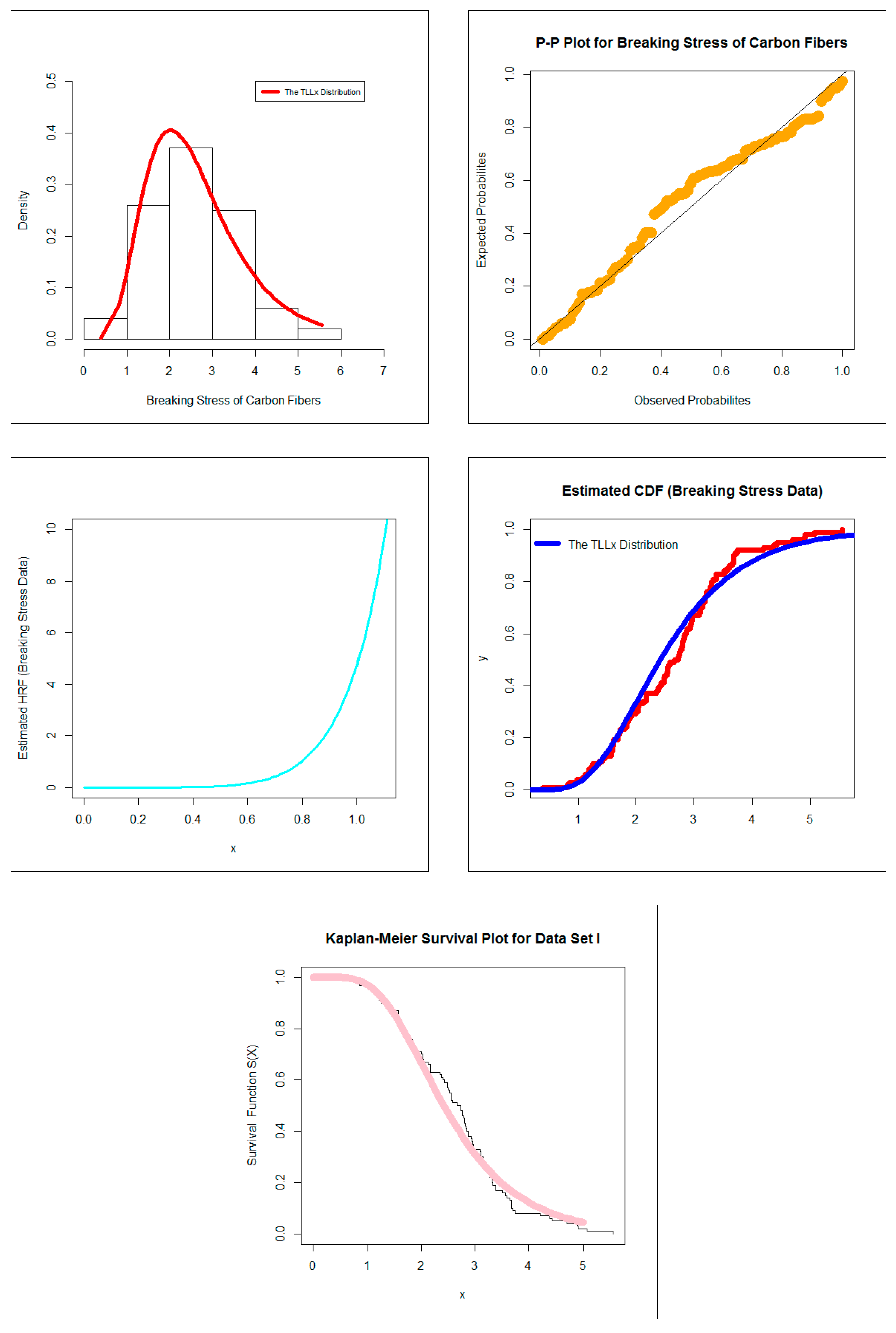
In physics and reliability analysis, the TLLx model can be applied in modeling the breaking stress data. As shown in Tables 5 and 9, the TLLx model showed its superiority against the standard Burr XII, the Marshall-Olkin Burr XII, the Topp Leone Burr XII, the Zografos-Balakrishnan Burr XII, the five parameters beta Burr XII, the beta Burr XII, the beta exponentiated Burr XII, the five parameters Kumaraswamy Burr XII and Kumaraswamy Burr XII distributions.
(4)
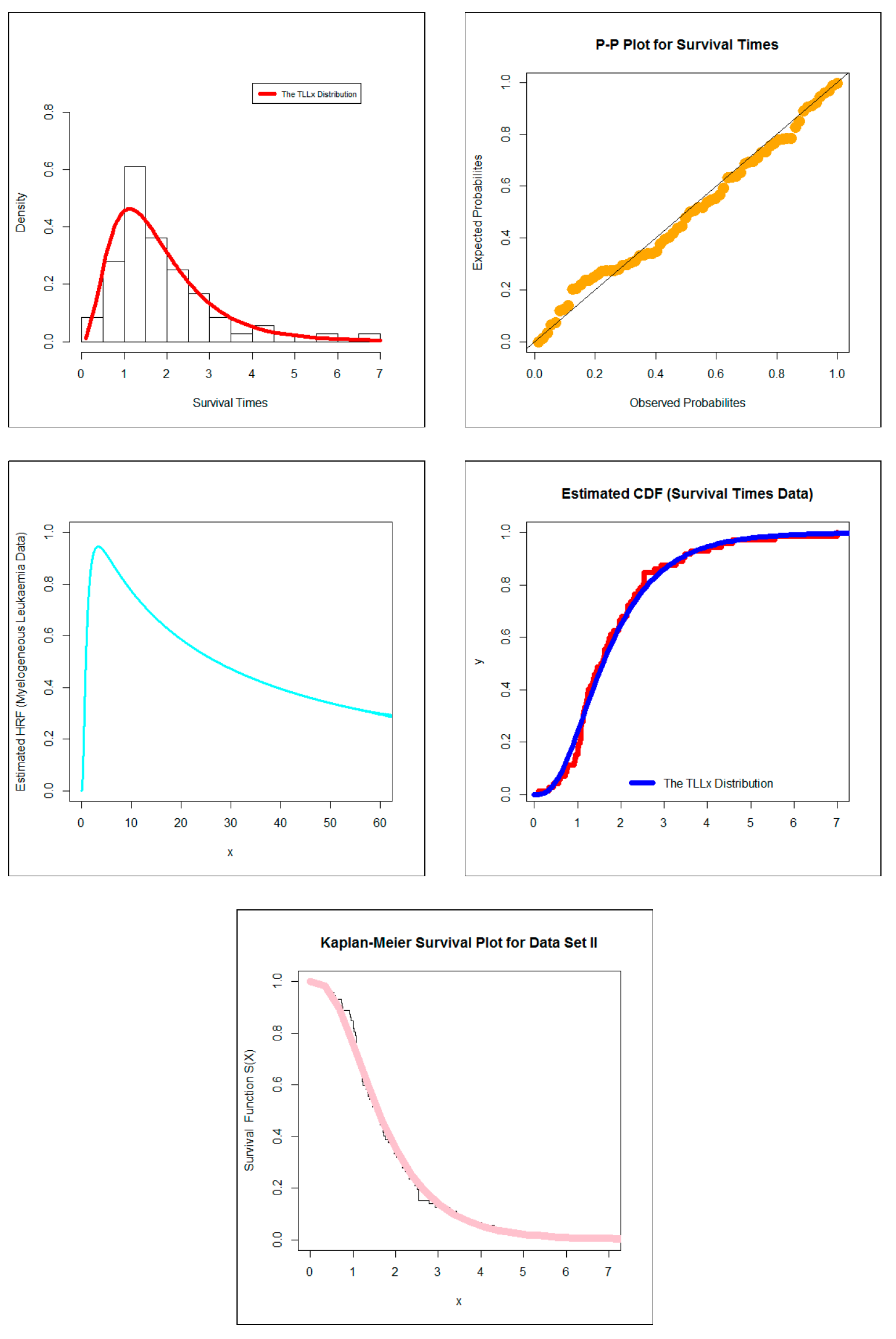
In survival analysis, the new model can be chosen in modeling the survival times data. As illustrated in Tables 6 and 10, the new model showed its superiority against all competitive models as mentioned in Table 4.
(5)
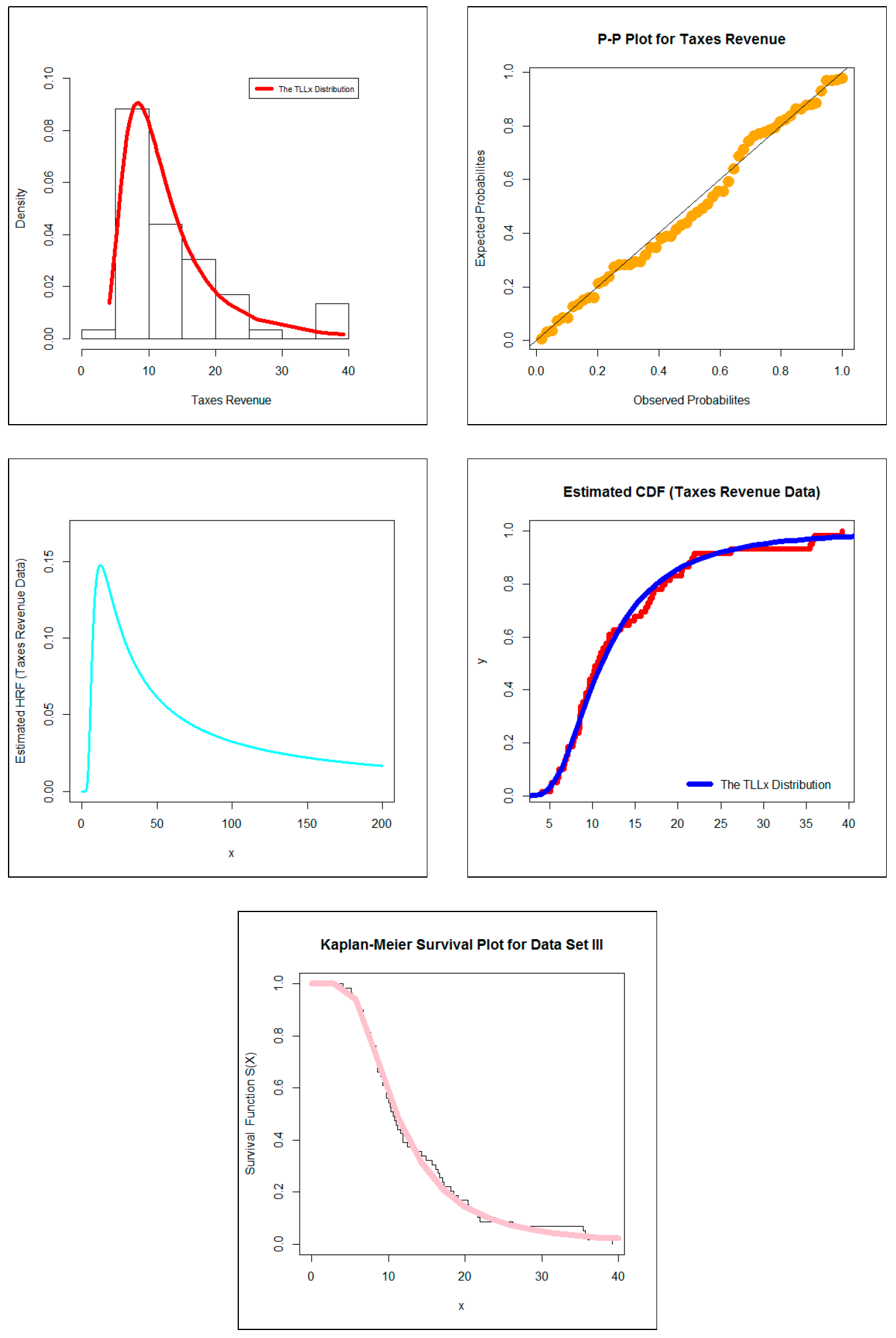
In econometrics, the new model can be used in modeling the taxes revenue data. From Tables 7 and 11 we note that the new model showed its superiority against many well-known competitive models.
(6)
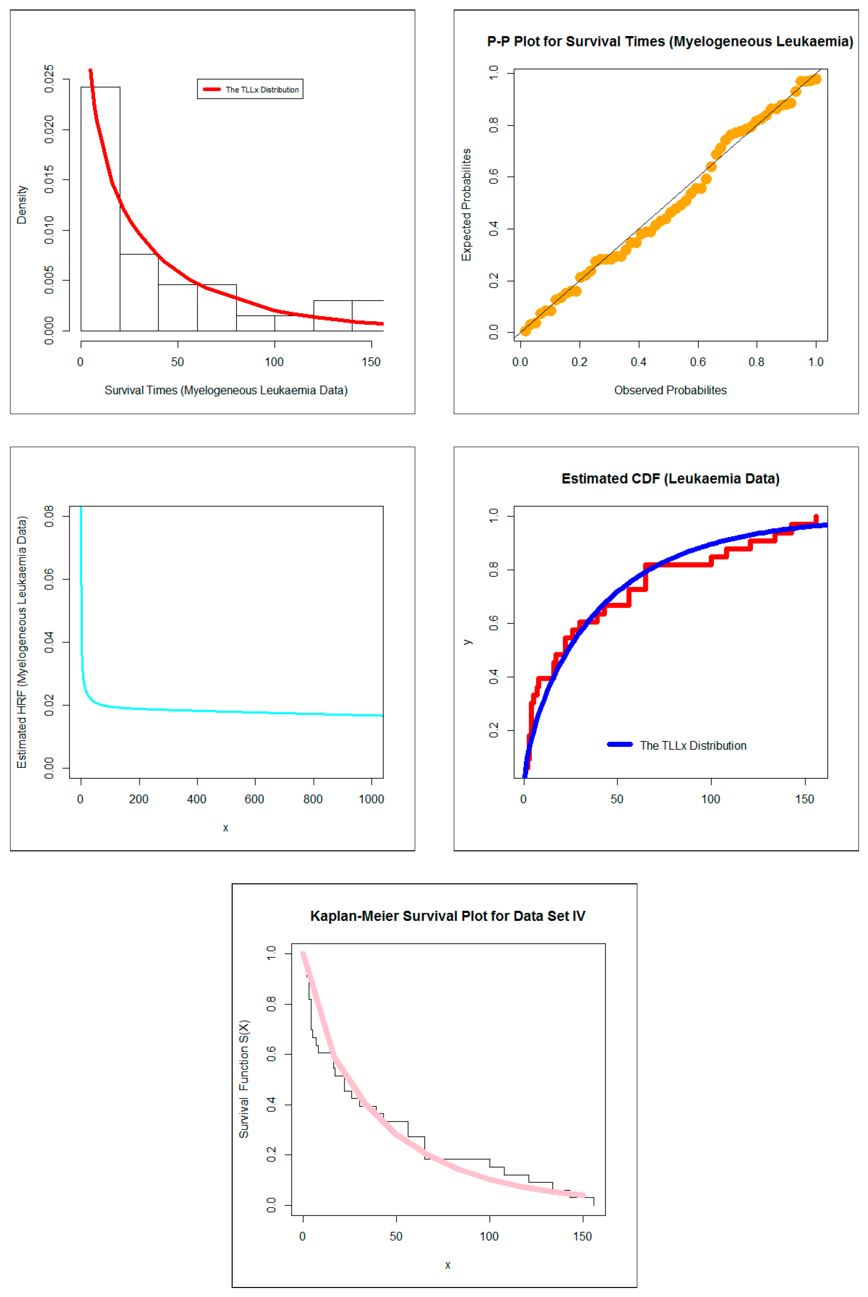
In the medicine field, our new model can be applied in modeling the acute myelogenous leukemia data. The new model showed its superiority against many competitive models such as the standard Burr XII, the Marshall-Olkin Burr XII, the Topp Leone Burr XII, the Zografos-Balakrishnan Burr XII, the five parameters beta Burr XII, the beta Burr XII, the beta exponentiated Burr XII, the five parameters Kumaraswamy Burr XII and Kumaraswamy Burr XII models as shown in Tables 8 and 12.

2. The New Model and Simple Type Copula-Based Construction

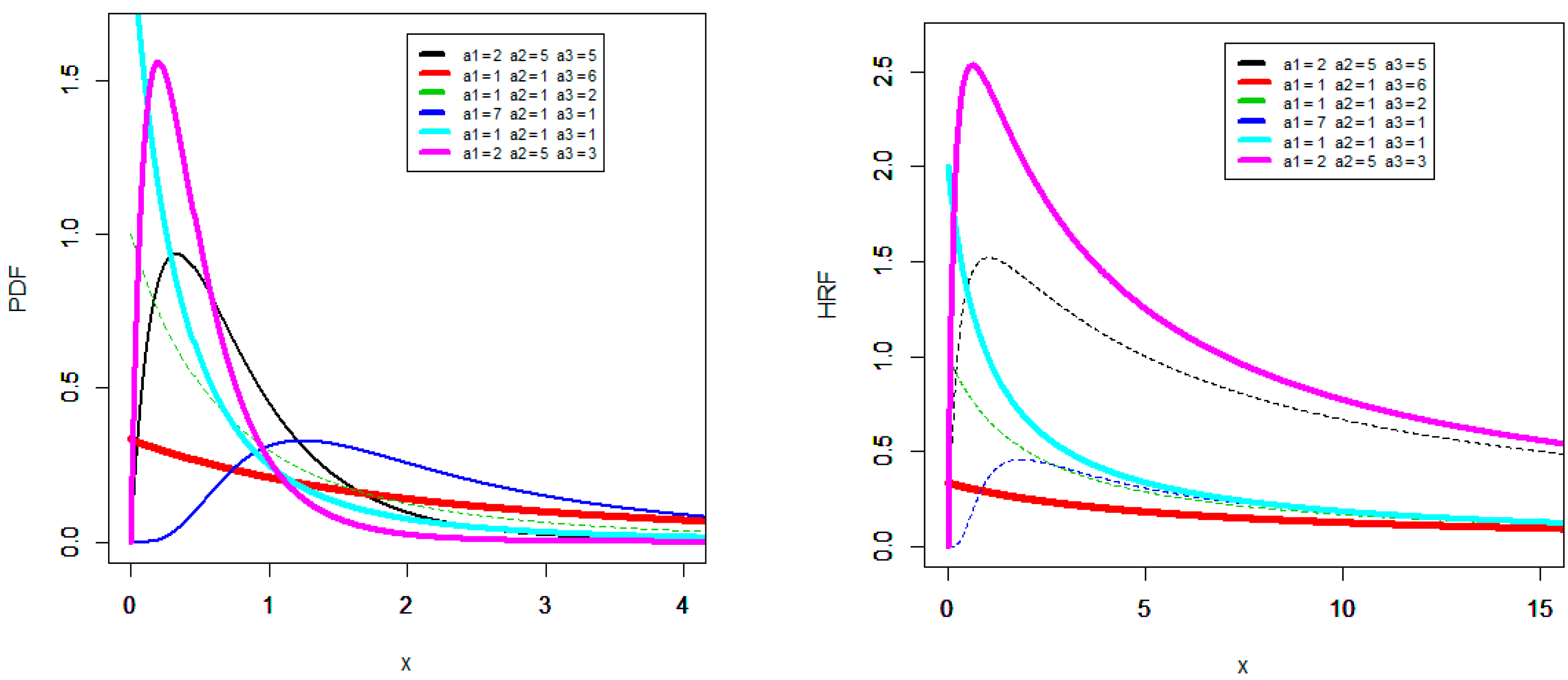
2.1. The New TLLx and Its Max-Mini Physical Interpretation.

Using the Topp-Leone G family originally proposed by [21] with following PDF:
f TL - G ( z ) = 2 α 1 g ( z ) [ G ( z ) ] α 1 [ 1 G ( z ) ] [ 2 G ( z ) ] α 1 1
We propose and study a new model called the Topp-Leone-Lx (TLLx). The PDF of the TLLx with parameters Ω _ = ( α 1 , α 2 , α 3 ) is given by:
f TLLx ( z , Ω _ ) = 2 α 1 α 2 α 3 ( 1 + z α 3 ) 2 α 2 1 [ 1 ( 1 + z α 3 ) 2 α 2 ] α 1 1 ,
and integrating (3) we have the new CDF as:
F TLLx ( z , Ω _ ) = [ 1 ( 1 + z α 3 ) 2 α 2 ] α 1 .
The TLLx distribution has a very important physical interpretation. Suppose a system has α 1 systems. All are systems working in parallel and each system has only two sub-systems working in series. Let Z ( i ,   j ) denote a variable of interest for the j t h sub-system associated with the i t h system. Suppose Z ( i ,   j ) are independent and identical random variables (IIDRVs) with CDF (2) [ G Lx ( z ; α 2 , α 3 ) ] . The variable Z ( i ,   j ) of interest for the system will be:
Z = max ( 1 < i < α 1 ) ( min j = 1 , 2 Z ( i ,   j ) ) ,
which can be called the “max-mini” physical interpretation. It is not difficult to show that the CDF of Z is (4). Figure 1 gives some plots of the TLLx PDF and HRF for selected parameter values. From Figure 1 (left panel), we note that the new PDF can be unimodal function with a heavy tail to the right (positive skewness). From Figure 1 (right panel), we note that the new hazard rate function (HRF) can be “upside-down” failure rate ( α 1 = 2 ,   α 2 = 5 , α 3 = 3 ), “decreasing” failure rate ( α 1 = 1 , α 2 = 1 , α 3 = 1 ) with many different shapes and “decreasing-constant” failure rate ( α 1 = 1 , α 2 = 1 , α 3 = 6 ).
The applicability and flexibility of the TLLx model given in (3) and (4) are illustrated via four real data applications. The results of the four applications which established the superiority of the TLLx model are listed in Tables 5–12. The corresponding figures of the four applications are presented in Figures 1–5.
For validating the TLLx model in applications and simulation, a new modified Chi-Square (Chi-S) ( χ 2 ) goodness-of-fit (GOF) test based on Nikulin-Rao-Robson (N-R-R) GOF test is used in the case of complete and censored data (general and right case) for the TLLx model.
The simulation results are listed in Tables 13–16. The different estimation methods are used for estimation of the model parameters and for assessing the finite sample behavior of the estimates. However, new goodness-of-fit test is used for validation of whether a certain model is suitable to fit a certain data set.

2.2. Copula via Morgenstern Gamily

First, we consider CDF for Morgenstern family of two rvs ( Z 1 , Z 2 ) which has the following form:
F λ ( z 1 , z 2 ) | ( | λ | 1 ) = F 1 ( z 1 ) { λ [ 1 F 1 ( z 1 ) ] [ 1 F 2 ( z 2 ) ] + 1 } F 2 ( z 2 )
where:
F 1 ( z 1 ) = F ( Ω _ α h ) ( z 1 ) = [ 1 ( 1 + z 1 α 3 ) 2 α 2 ] α 1 ,   and   F 2 ( z 2 ) = F ( Ω _ b h ) ( z 2 ) = [ 1 ( 1 + z 2 b 3 ) 2 b 2 ] b 1
and Ω _ α h = ( α 1 , α 2 , α 3 ) and Ω _ b h = ( b 1 , b 2 , b 3 ) , then we have a seven-dimension parameter model.

2.3. Copula Via Clayton Copula

2.3.1. The Bivariate Extension

The bivariate extension via clayton copula can be considered as a weighted version of the clayton copula, which is of the form:
C ( u ( z ) , v ( y ) ) | [ ( δ 1 + δ 2 ) > 0 ] = [ u ( z ) ( δ 1 + δ 2 ) + v ( y ) ( δ 1 + δ 2 ) 1 ] 1 δ 1 + δ 2 ,
where δ 1 and δ 2 are the clayton copula parameters. This is indeed a valid copula. Next, let us assume that Z TLLx ( Ω _ α h ) and Y TLLx ( Ω _ α h ) . Then, setting:
u ( z ) = u ( Ω _ α h ) ( z ) = [ 1 ( 1 + z α 3 ) 2 α 2 ] α 1 , h = 1 , 2 , 3 ,
and
v ( y ) = v ( Ω _ a h ) ( y ) = [ 1 ( 1 + y a 3 ) 2 a 2 ] a 1 ,   h = 1 , 2 , 3 ,
the associated CDF of bivariate TLLx type distribution is:
H ( z , y ) = ( { [ 1 ( 1 + z α 3 ) 2 α 2 ] α 1 } ( δ 1 + δ 2 ) + { [ 1 ( 1 + y a 3 ) 2 a 2 ] a 1 } ( δ 1 + δ 2 ) 1 ) 1 δ 1 + δ 2 .

2.3.2. The Multivariate Extension

A straightforward d -dimensional extension from the above will be:
H ( z 1 , z 2 , , z d ) = { h = 1 d [ 1 ( 1 + z i α 3 i ) 2 α 2 i ] α 1 i ( δ 1 + δ 2 ) + 1 d } 1 δ 1 + δ 2 .
Further future works could be done for studying the bivariate and the multivariate extensions of the TLLx model.

3. Some Properties

In this section, we investigate some mathematical properties of the TLLX model including the ordinary and incomplete moments (which are useful in deriving the mean deviations, Bonferroni curve, Lorenz curve and many other applications in econometrics and insurance), and quantile function and moment of the reversed residual life (RRL) which is useful in reliability analysis. Established algebraic expansions to determine some structural properties of this model can be more efficient than computing those directly by numerical integration of its PDF.
Let Z be a rv having the TLLx model in (3). The transformation t = 1 ( 1 + z α 3 ) α 2 can be used alongwith the binomial expansion to get the r t h moment of Z as:
μ r , Z ( z ) |   2 α 2 > r = α 1 α 3 r ω = 0 r ( 1 ) ω ( r ω ) B ( α 1 , 1 + ω r 2 α 2 )
where:
B ( ζ 1 , ζ 2 ) = 0 1 ω ζ 1 1 ( 1 ω ) ζ 2 1 d ω ,
is the complete beta function. The first three moments can be obtain by taking r = 1 ,   2 and 3 in (5) as follows:
μ 1 , Z ( z ) |   2 α 2 > 1 = α 1 α 3 [ B ( α 1 , 1 1 2 α 2 1 ) 1 α 1 ] ,
μ 2 , Z ( z ) |   α 2 > 1 = α 1 α 3 2 [ B ( α 1 , 1 α 2 1 ) + 1 α 1 2 B ( α 1 , 1 1 2 α 2 1 ) ] ,
and:
μ 3 , Z ( z ) |   2 α 2 > 3 = α 1 α 3 3 [ B ( α 1 , 1 3 2 α 2 1 ) + 3 B ( α 1 , 1 1 2 α 2 1 ) 3 B ( α 1 , 1 α 2 1 ) 1 α 1 ] ,
and the variance of the new model can be expressed as:
V a r ( Z ) = α 1 α 3 2 [ B ( α 1 , 1 α 2 1 ) α 1 B 2 ( α 1 , 1 1 2 α 2 1 ) ] .
The r t h incomplete moment ( μ r , Z ( t ) ) can be derived as:
μ r , Z ( t ) |   2 α 2 > r = 0 t z r f TLLx ( z , Ω _ ) d z = α 1 α 3 r ω = 0 r ( 1 ) ω ( r ω ) B t ( α 1 , 1 + ω r 2 α 2 ) ,
where:
B q ( ζ 1 , ζ 2 ) |   0 < q < 1 = 0 q ω ζ 1 1 ( 1 ω ) ζ 2 1 d t .
Moreover, in terms of the hypergeometric function 2 F 1 [ ] we can write:
B q ( ζ 1 , ζ 2 ) |   0 < q < 1 = ζ 1 1 q ζ 1 { 2 F 1 [ ζ 1 , 1 ζ 2 ; 1 + ζ 1 ; q ] } = m = 0 ( ζ 2 + 1 ) m q ζ 1 + m m ! ( ζ 1 + m ) .
The quantile function (QF) can be written as:
Z q = α 3 [ ( 1 q 1 α 1 ) 1 2 α 2 1 ] 0 < q < 1
The expression of z q can be used in simulating the TLLx model. The median of the TLLx model can be obtained at q = 0.5 . The n t h moment of RRL of any continuous rv is defined by:
Ω [ m ] ( τ ) = E [ ( τ Z ) m   | Z τ ,   τ , > 0 , m = 1 , 2 , ] = 1 F ( τ ) 0 τ ( τ z ) m d F ( z ) .
Then the m t h moment of RRL of Z can be expressed as:
Ω [ m ] ( τ ) = 1 F ( τ ) h , ω = 0 m ( 1 ) h m ! h ! ( m h ) ! α 1 α 3 m ( 1 ) ω ( m ω ) B τ ( α 1 , 1 + ω m 2 α 2 ) .

4. Different Methods of Estimation

4.1. Maximum Likelihood Estimation (MLE)

The log-likelihood function ( m ( Ω _ ) ) for Ω _ can be given by:
m ( Ω _ ) = m l o g 2 + m l o g α 1 + m l o g α 3 m l o g α 3 ( 2 α 2 + 1 ) h = 1 m l o g ( 1 + z ( h   :   m ) α 3 ) + ( α 1 1 ) h = 1 m l o g [ 1 ( 1 + z ( h   :   m ) α 3 ) 2 α 2 ]
where z ( h   :   m ) is the random variable which follow the TLLx but when we are dealing with a random sample of size m , and h refer to the summation index. The above m ( Ω _ ) can be numerically maximized. The components of the score vector U ( Ω _ ) where:
U ( Ω _ ) = Ω _ = ( α 1 m ( Ω _ ) , α 2 m ( Ω _ ) , α 3 m ( Ω _ ) ) T ,
are given by:
m ( Ω _ ) α 1 = m α 1 1 + h = 1 m l o g [ 1 ( 1 + z ( h   :   m ) α 3 ) 2 α 2 ] ,
m ( Ω _ ) α 2 = m α 2 1 + h = 1 m l o g   ( 1 + z ( h   :   m ) α 3 ) + 2 ( α 1 1 ) h = 1 m l o g ( 1 + z ( h   :   m ) α 3 ) [ ( 1 + z ( h   :   m ) α 3 ) 2 α 2 1 ] ,
and:
m ( Ω _ ) α 3 = m α 3 + ( 2 α 2 + 1 ) h = 1 m z ( h   :   m ) ( α 3 2 + α 3 z ( h   :   m ) ) h = 1 m 2 ( α 1 1 ) α 2 z ( h   :   m ) α 3 2 [ ( 1 + z ( h   :   m ) α 3 ) 2 α 2 + 1 ( 1 + z ( h   :   m ) α 3 ) ] .
respectively.

4.2. Maximum Product Spacing Estimator

Let D h ( α 1 , α 2 , α 3 ) be the uniform spacings of a random sample (RS) from the TLLx model defined by:
D h ( α 1 , α 2 , α 3 ) = F ( z ( h   :   m )   |   α 1 , α 2 , α 3 ) F ( z ( h 1   :   m )   |   α 1 , α 2 , α 3 ) | ( h = 1 , 2 , , m ) ,
where, F ( z 0   :   m   |   α 1 , α 2 , α 3 ) = 0 and F ( z ( m + 1   :   m )   |   α 1 , α 2 , α 3 ) = 1 .
Clearly
h = 1 m + 1 D h ( α 1 , α 2 , α 3 ) = 1 .
The MPSEs of α 1 , α 2 and α 3 are obtained by maximizing:
1 m + 1 h = 1 m + 1 l o g [ D h ( α 1 , α 2 , α 3 ) ] ,
with respect to α 1 , α 2 and α 3 .

4.3. Method of Least Square (LS) and Weighted Least Square (WLS) Estimation

Let F ( z ( h   :   m ) , Ω _ ) denote the CDF of TLLx version and let z 1 < z 2 < , , < z m be the m ordered random sample. The least square estimates are obtained by minimizing:
s ( Ω _ ) = h = 1 m [ F ( z ( h   :   m ) , Ω _ ) c ( m , h ) ] 2
where c ( m , h ) = h m + 1 . Now using CDF of TLLx we get:
s ( Ω _ ) = h = 1 m [ { 1 ( 1 + z ( h   :   m ) α 3 ) 2 α 2 } α 1 c ( m , h ) ] 2
The LSEs of Ω _ | ( Ω _ = α 1 , α 2 , α 3 ) are obtained by solving non-linear equations:
h = 1 m [ { 1 ( 1 + z ( h   :   m ) α 3 ) 2 α 2 } α 1 c ( m , h ) ] Λ 1 ( z ( h   :   m ) , Ω _ ) = 0
h = 1 m [ { 1 ( 1 + z ( h   :   m ) α 3 ) 2 α 2 } α 1 c ( m , h ) ] Λ 2 ( z ( h   :   m ) , Ω _ ) = 0
and:
h = 1 m [ { 1 ( 1 + z ( h   :   m ) α 3 ) 2 α 2 } α 1 c ( m , h ) ] Λ 3 ( z ( h   :   m ) , Ω _ ) = 0
where:
Λ 1 ( z ( h   :   m ) , Ω _ ) = α 1 { 1 ( 1 + z ( h   :   m ) α 3 ) 2 α 2 } α 1 1
Λ 2 ( z ( h   :   m ) , Ω _ ) = 2 α 1 α 2 α 3 2 z ( h   :   m ) { 1 ( 1 + z ( h   :   m ) α 3 ) 2 α 2 } α 1 1 ( 1 + z ( h   :   m ) α 3 ) 2 α 2 1
and:
Λ 3 ( z ( h   :   m ) , Ω _ ) = 2 α 1 { 1 ( 1 + z ( h   :   m ) α 3 ) 2 α 2 } α 1 1 ( 1 + z ( h   :   m ) α 3 ) 2 α 2 l o g ( 1 + z ( h   :   m ) α 3 )
The WLSEs can be obtained by minimizing:
ω ( Ω _ ) = h = 1 m ω ( m , h ) [ F TLLx ( z ( h   :   m ) , Ω _ ) c ( m , h ) ] 2
w.r.t. the parameters, where ω ( m , h ) = ( m + 1 ) 2 ( m + 2 ) h ( m h + 1 ) . Then we have:
ω ( Ω _ ) = h = 1 m ω ( m , h ) [ { 1 ( 1 + z ( h   :   m ) α 3 ) 2 α 2 } α 1 c ( m , h ) ] 2
The WLSEs are obtained by solving:
h = 1 m ω ( m , h ) [ { 1 ( 1 + z ( h   :   m ) α 3 ) 2 α 2 } α 1 c ( m , h ) ] Λ 1 ( z ( h   :   m ) , Ω _ ) = 0
h = 1 m ω ( m , h ) [ { 1 ( 1 + z ( h   :   m ) α 3 ) 2 α 2 } α 1 c ( m , h ) ] Λ 2 ( z ( h   :   m ) , Ω _ ) = 0 ,
and:
h = 1 m ω ( m , h ) [ { 1 ( 1 + z ( h   :   m ) α 3 ) 2 α 2 } α 1 c ( m , h ) ] Λ 3 ( z ( h   :   m ) , Ω _ ) = 0
The term Λ h ( Ω _ ) | ( h = 1 , 2 , 3 ) is same as defined above.

4.4. Method of Percentile Estimate

For (2), the QF is obtained as:
z p = α 3 [ ( 1 p 1 α 1 ) 1 2 α 2 1 ]
then the estimate of α 1 , α 2 , α 3 can be obtained by minimizing:
h = 1 m [ z ( h   :   m ) α 3 ( { 1 p h 1 α 1 } 1 2 α 2 1 ) ] 2 ,
w.r.t. α 1 , α 2 and α 3 . The percentile estimates are obtained by solving the following nonlinear equations:
h = 1 m [ z ( h ) α 3 1 p h 1 / α 1 ] p h 1 / α 1 l n p h ( 1 p h 1 / α 1 ) 2 = 0 ,
and:
h = 1 m [ z ( h ) α 3 1 p h 1 / α 1 ] 1 ( 1 p h 1 / α 1 ) = 0 ,
respectively, where p h = c ( m , h ) .

4.5. Method of Cramer-Von-Mises Estimation (CVME)

The CVME method of the parameters is based on the theory of minimum distance estimation. The CVME of the parameter α 1 , α 2 , and α 3 are obtained by minimizing the following expression w.r.t. α 1 , α 2 , and α 3 respectively:
CVM ( Ω _ ) = 1 12 m + h = 1 m [ F TLLx ( z ( h   :   m ) , Ω _ ) c ( 2 m , 2 h ) ] 2
where:
c ( 2 m , 2 h ) = 2 h 1 2 m
and:
CVM ( Ω _ ) = h = 1 m [ { 1 ( 1 + z ( h   :   m ) α 3 ) 2 α 2 } α 1 c ( 2 m , 2 h ) ] 2
The CVMEs of the parameters are obtained by solving the following non-linear equations:
h = 1 m [ { 1 ( 1 + z α 3 ) 2 α 2 } α 1 c ( 2 m , 2 h ) ] Λ 1 ( z ( h   :   m ) , Ω _ ) = 0
h = 1 m [ { 1 ( 1 + z α 3 ) 2 α 2 } α 1 c ( 2 m , 2 h ) ] Λ 2 ( z ( h   :   m ) , Ω _ ) = 0 ,
and:
h = 1 m [ { 1 ( 1 + z ( h   :   m ) α 3 ) 2 α 2 } α 1 c ( 2 m , 2 h ) ] Λ 3 ( z ( h   :   m ) , Ω _ ) = 0 ,
respectively.

4.6. Methods of Anderson-Darling (ADE)

The ADEs of the parameters ( α 1 , α 2 , α 3 ) are obtained by minimizing the following function, w.r.t. α 1 , α 2 and α 3 :
A D ( z ( h   :   m ) , α 1 , α 2 , α 3 ) = m 1 m h = 1 m ( 2 h 1 ) [ l n F TLLx ( z ( h   :   m ) , Ω _ ) ] ) + l n F ¯ TLLx ( z m + 1 h   :   m , Ω _ ) .
The respective estimate of α 1 , α 2 , α 3 is obtained by solving the following non-linear equations:
h = 1 m ( 2 h 1 ) [ ζ 1 ( z ( h   :   m ) , α 1 , α 2 , α 3 ) F ( z ( h   :   m ) , α 1 , α 2 , α 3 ) ζ 1 ( z ( h   :   m ) , α 1 , α 2 , α 3 ) F ¯ ( z ( h   :   m ) , α 1 , α 2 , α 3 ) ] = 0 ,
and:
h = 1 m ( 2 h 1 ) [ ζ 2 ( z ( h   :   m ) , α 1 , α 2 , α 3 ) F ( z ( h   :   m ) , α 1 , α 2 , α 3 ) ζ 2 ( z ( h   :   m ) , α 1 , α 2 , α 3 ) F ¯ ( z ( h   :   m ) , α 1 , α 2 , α 3 ) ] = 0 .
h = 1 m ( 2 h 1 ) [ ζ 3 ( z ( h   :   m ) , α 1 , α 2 , α 3 ) F ( z ( h   :   m ) , α 1 , α 2 , α 3 ) ζ 3 ( z ( h   :   m ) , α 1 , α 2 , α 3 ) F ¯ ( z ( h   :   m ) , α 1 , α 2 , α 3 ) ] = 0 .

5. Monte Carlo (MC) Simulation Study

In this section, the performances of the computed estimators in previous section are investigated by conducting Monte Carlo simulations. The simulation has been performed for the different variation of the model parameters as well as sample size. In particular, we took four choices of ( Ω _ ) | ( 0.5 , 0.5 , 0.5 ) , ( 0.5 , 1.0 , 1.5 ) , ( 1.5 , 2.0 , 2.5 ) , ( 2.0 , 3.0 , 3.0 ) along with m | ( m = 10 , 20 , 30 , 50 , 100 , 200 ) . The average means square error (AMSEs) for the considered variations are reported based on the 5000 replications, see Table 1, Table 2 and Table 3.
From these extensive simulation study, it has been noticed that all the estimators satisfy the property of consistency as m increases in all the considered setup. Among the employed different methods of estimation, maximum likelihood estimation method is more efficient for all the parameters. The following trends have been observed:
R ( Ω _ ) m l < R ( Ω _ ) c v < R ( Ω _ ) a d < R ( Ω _ ) w l s < R ( Ω _ ) l s < R ( Ω _ ) m p < R ( Ω _ ) p c .

6. Modeling Real Data

Four real and different data sets are modeled and analyzed to illustrate the importance, potentiality and flexibility of the TLLx model. We compare the TLLx distribution with the following models listed in Table 4:
The observations of the four data sets are given in Appendix A. First, we sketch the total time test (TTT) plot (see [21]) for all real data sets in Figure 1. These plots indicate that the empirical HRFs of data sets I, II, III are increasing and bathtub for data set IV. Then, we consider the following GOF statistics:
  • The Akaike Information Criterion (A_IC),
  • Bayesian_IC (B_IC),
  • Hannan-Quinn_IC (HQ_IC), and
  • Consistent Akaike_IC (CA_IC).
The lowest values of these Criterion refer to the best model. Table 5, Table 6, Table 7 and Table 8 give the MLEs, standard errors (SEs), confidence intervals (CIs) for the data sets I, II, III and IV, respectively. Table 9, Table 10, Table 11 and Table 12 give the B_IC, A_IC, CA_IC and HQ_IC, respectively. Based on the values in Table 9, Table 10, Table 11 and Table 12 and Figure 2, Figure 3, Figure 4 and Figure 5, the TLLx model provides the best fit in the four applications with smallest values for the above-mentioned criterion. The TLLx model has only three parameters. However, all other competitive models have at least three parameters. The model with a smaller number of parameters is favorable especially if it gives a better fit. The TLLx model has this advantage and this is illustrated in Table 9, Table 10, Table 11 and Table 12. The TLLx model has the lowest value of the following criteria B_IC, A_IC, CA_IC and HQ_IC. From Table 9 the TLLx model has:
  • B_ IC = 306 , A_ IC = 298 , CA_ IC = 299 and HQ_ IC = 302 .
  • From Table 10 the TLLx model has
  • B_ IC = 212 , A_ IC = 205 , CA_ IC = 206 and HQ_ IC = 208 .
  • From Table 11 the TLLx model has
  • B_ IC = 389 , A_ IC = 383 , CA_ IC = 383 and HQ_ IC = 385 .
  • From Table 12 the TLLx model has
  • B_ IC = 314 , A_ IC = 313 , CA_ IC = 318 and HQ_ IC = 315 .
So, it is recommended to use the TLLx model instead of all other competitive models.
The bold values in Table 9, Table 10, Table 11 and Table 12 show that the new TLLx model is the best model among all other competitive models.
Figure 3 shows that the TLLx model has a very adequate fitting to the empirical function for the data set I, Figure 4 shows that the TLLx model has a very adequate fitting to the empirical function for the data set II, Figure 5 shows that the TLLx model has a very adequate fitting to the empirical function for the data set III, Figure 6 shows that the TLLx model has a very adequate fitting to the empirical function for the data set IV.

7. Assessing the Performance of the Maximum Likelihood Estimations: Case of Complete Data

Using Barzilai-Borwein (BB) algorithm, we simulate the TLLx model where sample sizes are m = 30 , m = 100 , m = 250 , m = 400 , and parameter values α 1 = 0.7 , α 2 = 2.6 , α 3 = 1.9 . The averages of the simulated values (AVs) of the estimators α ^ 1 , α ^ 2 and α ^ 3 and their corresponding MSEs are presented in Table 13 which indicates that when m increases the MSEs decreases and decay to zero.

8. Assessing the Performance of the Maximum Likelihood Estimations: Case of Censored Data

8.1. The Maximum Likelihood Estimation (MLE)

For h (an individual); Υ [ h ] is the lifetime and [ h ] is the censorship time, where Υ [ h ] and [ h ] are independent rvs. Consider a data set of m independent observations and let τ h | ( h = 1 , 2 , m ) = m i n ( Υ [ h ] , [ h ] ) .
Censorship case is assumed to be non-informative one, which means that the distribution of [ h ] does not depend in any way on the unknown parameters of Υ [ h ] . The likelihood function in the case of censored data can be written as:
L ( τ , Ω _ ) = h = 1 m φ ( Υ ( h ) ) ( τ h , Ω _ ) S TLLx ( τ h , Ω _ ) , |   ( Υ ( h ) = 1 { Υ [ h ] [ h ] } )
where S TLLx ( τ h , Ω _ ) = 1 − F TLLx ( τ h , Ω _ ) . In our case, let Υ [ h ] be a rv distributed with the vector of parameters Ω _ , so the likelihood function, L ( τ , Ω _ ) , reduces to:
L ( τ , Ω _ ) = h = 1 m [ 2 α 1 α 2 α 3 1 ( 1 + τ h α 3 ) 2 α 2 1 × [ 1 ( 1 + τ h α 3 ) 2 α 2 ] α 1 1 × { 1 [ 1 ( 1 + τ h α 3 ) 2 α 2 ] α 1 } 1 ] Υ ( h ) { 1 [ 1 ( 1 + τ h α 3 ) 2 α 2 ] α 1 } ,
and the logL function is given:
l ( τ , Ω _ ) = r l n ( 2 α 1 α 2 α 3 l ) ( 2 α 2 + 1 ) h = 1 m Υ ( h ) l n ( 1 + τ h α 3 ) + ( α 1 1 ) h = 1 m Υ ( h ) l n [ 1 ( 1 + τ h α 3 ) 2 α 3 ] h = 1 m Υ ( h ) l n { 1 [ 1 ( 1 + τ h α 3 ) 2 α 3 ] α 1 } + h = 1 m l n { 1 [ 1 ( 1 + τ h α 3 ) 2 α 3 ] α 1 } ,
and then:
l ( τ , Ω _ ) = r [ l o g ( 2 α 1 ) l o g ( α 3 ) + l o g ( α 2 ) ] ( 2 α 2 + 1 ) ( h ϕ ) l n ( 1 + τ h α 3 ) + ( α 1 1 ) ( h ϕ ) l n [ 1 ( 1 + τ h α 3 ) 2 α 2 ] ( h ϕ ) l n { 1 [ 1 ( 1 + τ h α 3 ) 2 α 2 ] α 1 } + ( h ) l n { 1 [ 1 ( 1 + τ h α 3 ) 2 α 2 ] α 1 } ,
where r refers to the number of failures, and ϕ denote the sets of censored and uncensored observations, respectively. The MLE Ω _ ^ of Ω _ can be obtained by solving the following system:
l ( τ , Ω _ ) α 2 = r α 2 2 ( h ϕ ) l n ( 1 + τ h α 3 ) + ( h ϕ ) 2 α 1 ( 1 + τ h α 3 ) 2 α 2 l o g ( 1 + τ h α 3 ) [ 1 ( 1 + τ h α 3 ) 2 α 2 ] α 1 1 1 [ 1 ( 1 + τ h α 3 ) 2 α 2 ] α 1 ( h ) 2 α 1 ( 1 + τ h α 3 ) 2 α 2 l o g ( 1 + τ h α 3 ) [ 1 ( 1 + τ h α 3 ) 2 α 2 ] α 1 1 1 [ 1 ( 1 + τ h α 3 ) 2 α 2 ] α 1 = 0 ,
l ( τ , Ω _ ) α 3 = r α 3 ( 2 α 2 + 1 ) ( h ϕ ) l n ( 1 + τ h α 3 2 ) ( α 1 1 ) ( h ϕ ) 2 α 2 τ h ( 1 + τ h α 3 ) 2 α 2 1 α 3 2 [ 1 ( 1 + τ h α 3 ) 2 α 2 ] ( h ϕ ) 2 α 1 α 2 τ h ( 1 + τ h α 3 ) 2 α 2 1 [ 1 ( 1 + τ h α 3 ) 2 α 2 ] α 1 1 α 3 2 { 1 [ 1 ( 1 + τ h α 3 ) 2 α 2 ] α 1 } + ( h ) 2 α 1 α 2 τ h ( 1 + τ h α 3 ) 2 α 2 1 [ 1 ( 1 + τ h α 3 ) 2 α 2 ] α 1 1 α 3 2 { 1 [ 1 ( 1 + τ h α 3 ) 2 α 2 ] α 1 } = 0 .
The Markov chain MC (MCMC) and the BB algorithm can be used in this regard.

8.2. Simulations: Right Censored Case

Consider m = 30 , 100 , 250 , 400 and α 1 = 0.75 , α 2 = 2.45 and α 3 = 1.5 . The AVs of the MLEs α ^ 1 , α ^ 2 , α ^ 3 and their MSEs are calculated and listed in Table 14. From Table 14, we can see that the mean MSEs decreases and decay to zero which confirms the convergence property of the MLEs.

9. The Modified GOF Test

9.1. The N-R-R GOF Test

For testing H [ 0 ] where Υ 1 , Υ 2 , , Υ m is a RS from a parametric model F Ω _ ( τ ) , we have:
H [ 0 ]   :   P { Υ ( h ) τ } = F Ω _ ( τ ) ,   τ R ,   Ω _ = ( Ω _ 1 , Ω _ 2 , , Ω _ s ) T ,
Reference [22] and then Reference [23] proposed the N-R-R ( Y 2 ) statistic for this purpose. Let Υ 1 , Υ 2 , , Υ m be grouped in r sub-intervals I 1 , I 2 , , I r as:
I κ = ] a ( κ 1 ) ; a ( κ ) ]   |   ( κ = 1 , 2 , , r ) ,
which are mutually disjoint. The limits a ( ) of the intervals I κ are calculated such that:
p κ ( Ω _ ) = a ( κ 1 ) a ( κ ) f Ω _ ( τ ) d τ ,
So:
a ( κ ) = F 1 ( κ r ) | ( κ = 1 , 2 , , r 1 ) .
Let the vector frequencies be:
u κ = ( u 1 , u 2 , , u r ) T ,
where:
u κ = h = 1 m 1 { τ h I κ }   | ( κ = 1 , , r ) .
The N-R-R statistic ( Y 2 ( Ω _ ^ m ) ) can be derived as:
Y 2 ( Ω _ ^ m ) = χ m 2 ( Ω _ ^ m ) + m 1 T ( Ω _ ^ m ) ( Ι ( Ω _ ^ m ) J ( Ω _ ^ m ) ) 1 ( Ω _ ^ m ) ,
where Ι ( Ω _ ^ m ) is the estimated Fisher information matrix (FIM), where:
χ m 2 ( Ω _ ) = ( u 1 m p 1 ( Ω _ ) m p 1 ( Ω _ ) , u 2 m p 2 ( Ω _ ) m p 2 ( Ω _ ) , , u r m p r ( Ω _ ) m p r ( Ω _ ) ) T ,
and J ( Ω _ ) is the FIM but for grouped data which can be defined as J ( Ω _ ) = B ( Ω _ ) T B ( Ω _ ) ,   where:
B ( Ω _ ) = [ 1 p h p h ( Ω _ ) μ ] r × s | ( h = 1 , 2 , , r ) ,
then:
l ( Ω _ ) = ( l 1 ( Ω _ ) , l 2 ( Ω _ ) , , l s ( Ω _ ) ) T ,
with:
l k ( Ω _ ) = h = 1 r u h p h Ω _ k p h ( Ω _ ) | ( k = 1 , 2 , s ) ,
where Y 2 ~ χ r 1 2 Chi-Square with D.F. = r 1 .

9.2. N-R-R Statistic for the TLLx Model

To test H [ 0 ] that a certain RS belongs to the TLLx model, we calculate the N-R-R ( Y 2 ) statistic of N = 10 , 000 simulated samples m = 30 , 50 , 100 , 250 and m = 400 .   ε = 0.02 , 0.05 , 0.01 , 0.1 , the average numbers of the non-rejection times of H [ 0 ] is calculated when Y 2 χ ε 2 ( r 1 ) in Table 15 from which we note that the calculated ε h are close to initial ε h which means that the proposed GOF test is suited to the TLLx model.
.

10. Applications to Real Data

Strengths of Glass Fibers

The strengths data (see [24]) are fitted by TLLx model. Using the BB algorithm, the have α ^ 1 = 4.2578 , α ^ 2 = 1.2406 , α ^ 3 = 1.00897 and the estimated FIM Ι ( Ω _ ^ m ) expressed as:
Ι ( Ω _ ^ m ) = ( 0.1005487 0.0345872 9.254871 0 13.52489 78.254901 0 0 215.85473 )
and then the N-R-R statistic:
Y 2 = 11.13254   and   χ 0.05 2 ( 7 1 ) = 12.59159
which confirms that strengths data can be modeled by TLLx model.

11. GOF Test for Right Censored Data

In case of right censored data, the approaches proposed by [25,26] are suggested to be used. Consider:
H [ 0 ]   :   F ( τ ) F 0 = { F 0 ( τ , Ω _ ) , τ R ( 1 ) ,   Ω _ Θ R ( s ) } ,
where Ω _ = ( Ω 1 , Ω 2 , , Ω s ) T Θ R s is an unknown parameter of a certain model and 0 is a certain CDF with the support ( 0 , ) . Let [ 0 , τ ] be a finite time interval, where r is the maximum time of a certain study, and divide it into k > s smaller intervals ( a ( κ 1 ) , a ( κ ) ] = I κ , where:
0 = < a ( 0 ) < a ( 1 ) < < a ( k 1 ) < a ( k ) = + .
Then a ^ k can be given by:
a ^ k = Φ 1 [ E k k = 1 h 1 Φ ( Υ ( ) , Ω ^ _ ) m h + 1 , Ω ^ _ ] , a ^ k = Υ ( m ) |   k = 1 , , k
where Φ 1 is the inverse of cumulative HRF, Υ ( h ) is the i t h element in the ordered statistics (OS) ( Υ ( 1 ) , Υ ( 2 ) , , Υ ( m ) ) and:
E k = ( m + 1 h ) Φ ( a ^ ( k ) , Ω ^ _ ) + k = 1 h 1 Φ ( Υ ( ) , Ω ^ _ ) .
Usually in real application we fix k. [27] and [28] give some recommendations for the choice of intervals. The test is based on the vector:
Z = ( Z 1 , Z 2 , , Z k ) T , Z κ = 1 m ( U κ e κ ) | ( κ = 1 , 2 , , k ) ,
where e κ represents expected numbers of failures and U κ is the numbers of observed failures in these intervals. The test statistic for H [ 0 ] can be written as:
Y m 2 = Z 2 ( ^ ) 1 Z ,
where:
( ^ ) 1 = ( P ^ k ) 1 + ( e ^ ) 1 P ^ T ( G ^ ) 1 e ^ ( P ^ k ) 1 ,
and
G ^ = i ^ e ^ ( P ^ k ) 1 ( e ^ ) T .
Or, test statistic ( Y m 2 ) can be written as:
Y m 2 = κ = 1 k ( U κ e κ ) 2 U κ + Q ,
where:
P ^ k = m 1 U κ ,   G ^ = [ g ^ ( ) ] s × s ,
U κ = ( h : z h I k ) Υ ( h ) ,   Q = ( W ^ ) T ( G ^ ) 1 W ^ ,
e ^ ( k ) = m 1 ( h : z h I k ) Υ ( h ) Ω _ l n [ Φ ( h ) ( τ h , Ω _ ^ ) ] ,
W ^ = k = 1 k e ^ ( k ) ( P ^ k ) 1 Z k , , = 1 , s ,
W ^ = ( W ^ 1 , W ^ 2 , , W ^ s ) T ,
I ^ = m 1 h = 1 m Y ( h ) Ω _ ( ) l n [ Φ ( h ) ( τ h , Ω _ ^ ) ] ,
g ^ ( ) = i ^ ( ) k = 1 k e ^ ( k ) e ^ ( k ) ( P ^ k ) 1 ,
and
e ^ ( k ) = m 1 ( h : z h I k ) Υ ( h ) Ω _ l n [ Φ ( h ) ( τ h , Ω _ ^ ) ] .
Details about the matrices W ^ and I ^ are given in [29] and can easily be derived (see [29]). The limit distribution for Y m 2 is Chi-Square model with D . F . = r = r a n k ( ) = t r ( ( ) 1 ) .

GOF Test for the TLLx Model in Case of Censored Data

Suppose H [ 0 ] is examined, that is, the failure rate Υ ( h ) follows the TLLx, the survival function is:
S Ω _ ( τ ) = 1 [ 1 ( 1 + z α 3 ) 2 α 2 ] α 1 .
Then:
T L L x ( τ , Ω _ ) = l n S Ω _ ( τ ) = l n { 1 [ 1 ( 1 + z α 3 ) 2 α 2 ] α 1 } ,
where:
E k = ( h : z h > a ( k ) ) [ ( a ( k ) τ h , Ω _ ^ ) ( a ( k 1 ) , Ω _ ^ ) ] .
Under such choice of intervals, we have a constant value of e κ = E k k   k .

12. GOF Test for the TLLx Model in Case of Censored Data

12.1. Simulation Study

To test H [ 0 ] that a RS has arisen from a TLLx model, we calculate Y m 2 the N-R-R statistic of N = 10000 and m = 30 , m = 150 , m = 250 , m = 40 , ε = 0.02 ,   0.05 ,   0.01 ,   0.1 and the mean of the number of no rejections of H [ 0 ] | ( Y m 2 χ ε 2 ( r ) ) . Then we present the results of the empirical values and the corresponding theoretical values in Table 16. From Table 16, we can say that the proposed GOF test shows that the censored data fit the TLLx model.

12.2. Application to Real Data

Data of aluminum reduction cells

Consider data of aluminum reduction cells of [30] {0.468, 0.838, 0.853, 0.725, 0.965, 1.142, 1.304, 1.139, 1.317, 1.427, 1.554, 1.764, 1.776, 1.990, 2.010, 2.224, 1.658, 2.279*, 2.244*, 2.286*. (* censoring).} comes from the TLLx model, the MLEs Ω _ ^ are α ^ 1 = 2.0058 , α ^ 2 = 1.8457 , α ^ 3 = 1.8245 . Choose number of classes r = 4 , then, the element of Y m 2 are listed in Table 17.
Where:
Y m 2 = 9.09548   and   χ 0.05 2 ( 4 ) = 9.4877 > Y m 2
which means that this data can be modeled by the TLLx model.

13. Conclusions

In this work, we first introduced a new univariate version of the Lomax model called the TLLx model as well as a simple type copula-based construction via Morgenstern family and via Clayton copula for introducing a new bivariate and multivariate type extension of the TLLx model. The new PDF can be unimodal function with a heavy tail to the right (positive skewness). The new HRF can be “upside-down” failure rate “decreasing” failure rate with many different shapes and “decreasing-constant” failure rate. Some mathematical properties of the TLLx model are derived. The model parameters are estimated via different estimation methods such as maximum likelihood method, maximum product spacing method, method of least square and weighted least square estimation, method of percentile estimation, method of Cramer-Von-Mises estimation and methods of Anderson-Darling. The different estimation methods are used for estimation of the model parameters and assessing of the finite sample behavior of their estimators. For comparing the estimation methods, MCMC simulations are performed. The applicability and flexibility of the TLLx model is illustrated via four real data applications. We constructed a modified Chi-Square goodness-of-fit test based on Nikulin-Rao-Robson test in the case of complete and censored samples for the TLLx model. Simulation studies are performed using applications on real data. The new goodness-of-fit test is used for validation.

Author Contributions

A.S.Y.: Software. H.G.: Validation. R.M.A.: Conceptualization & Methodology. R.H.: Conceptualization & Methodology. M.M.A. & H.M.Y.: Writing review, editing & Project administration. All authors have read and agreed to the published version of the manuscript.

Funding

This research was funded by the Deanship of Scientific Research at Princess Nourah bint Abdulrahman University through the Fast-track Research Funding Program.

Conflicts of Interest

The authors declare no conflict of interest.

Appendix A

Data set I (called breaking stress data see [31]): 0.98, 5.56, 2.83, 3.68, 2.00, 3.51, 0.85, 1.61, 3.28, 2.95, 5.08, 0.39, 1.57, 3.19, 4.90, 2.74, 2.73, 2.50, 3.60, 3.11, 2.93, 2.85, 2.77, 2.76, 1.73, 2.48, 3.22, 3.70, 3.27, 2.87, 1.47, 3.11, 4.42, 2.81, 3.15, 1.92, 1.84, 1.22, 2.17, 1.61, 2.12, 3.09, 2.97, 4.20, 2.35, 1.41, 1.59, 1.12, 1.69, 2.79, 1.89, 1.87, 3.39, 3.33, 2.55, 3.68, 3.19, 1.71, 1.25, 4.70, 2.88, 3.68, 1.08, 3.22, 3.75, 2.96, 2.55, 2.59, 2.97, 1.57, 2.17, 4.38, 2.03, 2.82, 2.53, 3.31, 2.38, 1.36, 0.81, 1.17, 1.84, 12.40, 3.15, 2.67,3.31, 2.81, 2.56, 2.17, 4.91, 1.59, 1.18, 2.48, 2.03, 1.69, 2.43, 3.39, 3.56, 0.80, 2.05, 3.65.
Data set II (called survival times in days and reported by [32]): 0.1, 0.33, 1.08, 1.08, 1.08, 0.44, 0.56, 0.59, 0.72, 0.74, 0.77, 2.54, 2.78, 2.93, 3.27, 3.42, 0.92, 0.93, 0.96, 1, 1, 1.02, 1.05, 1.07, 07, 1.09, 1.12, 1.13, 1.15, 1.36, 1.39, 1.44, 1.83, 1.95, 1.96, 1.97, 2.02, 1.16, 1.2, 1.21, 1.22, 1.22, 1.24, 1.3, 1.34, 2.13, 1.46, 1.53, 1.59, 1.6, 1.63, 1.63, 1.68, 1.71, 1.72, 1.76, 2.15, 2.16, 2.22, 2.3, 2.31, 2.4, 2.45, 2.51, 2.53, 2.54, 3.47, 3.61, 4.02, 4.32, 4.58, 5.55}.
Data set III (called taxes revenue data in 1000 million Egyptian pounds): 5.9, 20.4, 13.3, 8.5, 21.6, 14.9, 16.2, 17.2, 7.8, 6.1, 9.2, 10.2, 9.6, 18.5, 5.1,6.7, 17, 9.2, 26.2, 21.9,16.7, 21.3, 35.4, 14.3, 8.6, 9.7, 39.2, 35.7, 15.7, 9.7, 10, 4.1, 36, 8.5, 8, 8.5, 10.6, 19.1, 20.5, 7.1, 7.7, 18.1, 16.5, 8.4, 11, 11.6, 11.9, 5.2, 6.8, 11.9, 7, 8.6,12.5, 10.3, 11.2, 6.1, 8.9, 7.1, 10.8}.
Data set IV (called leukemia data and represents the survival times in weeks of 33 patients suffering from acute Myelogenous Leukemia.): 65, 56, 26, 22, 1, 1, 5, 65, 16, 22, 3, 4, 2, 3, 56, 65, 17, 7, 156, 8, 4, 3, 30, 4, 100, 134, 16, 108, 121, 4, 39, 143, 43.

References

  1. Lomax, K.S. Business failures: Another example of the analysis of failure data. J. Am. Stat. Assoc. 1954, 49, 847–852. [Google Scholar] [CrossRef]
  2. Burr, I.W. Cumulative Frequency Functions. Ann. Math. Stat. 1942, 13, 215–232. [Google Scholar] [CrossRef]
  3. Burr, I.W. On a general system of distributions, III. The simple range. J. Am. Stat. Assoc. 1968, 63, 636–643. [Google Scholar] [CrossRef]
  4. Burr, I.W. Parameters for a general system of distributions to match a grid of alpha 3 and alpha 4. Commun. Stat. 1973, 2, 1–21. [Google Scholar] [CrossRef]
  5. Rodriguez, R.N. A guide to the Burr type XII distributions. Biometrika 1977, 64, 129–134. [Google Scholar] [CrossRef]
  6. Burr, I.W.; Cislak, P.J. On a general system of distributions: I. Its curve-shaped characteristics; II. The sample median. J. Am. Stat. Assoc. 1986, 63, 627–635. [Google Scholar] [CrossRef]
  7. Tadikamalla, P.R. A look at the Burr and related distributions. Int. Stat. Rev. 1980, 48, 337–344. [Google Scholar] [CrossRef]
  8. Cordeiro, G.M.; Yousof, H.M.; Ramires, T.G.; Ortega, E.M.M. The Burr XII system of densities: Properties, regression model and applications. J. Stat. Comput. Simul. 2018, 88, 432–456. [Google Scholar] [CrossRef]
  9. Abdul-Moniem, I.B.; Abdel-Hameed, H.F. On exponentiated Lomax distribution. Int. J. Math. Arch. 2012, 3, 2144–2150. [Google Scholar] [CrossRef]
  10. Ghitany, M.E.; AL-Awadhi, F.A.; Alkhalfan, L.A. Marshall-Olkin extended Lomax distribution and its applications to censored data. Commun. Stat. Theory Methods 2007, 36, 1855–1866. [Google Scholar] [CrossRef]
  11. Lemonte, A.J.; Cordeiro, G.M. An extended Lomax distribution. Statistics 2013, 47, 800–816. [Google Scholar] [CrossRef]
  12. Cordeiro, G.M.; Ortega, E.M.M.; Popovic, B.V. The gamma-Lomax distribution. J. Stat. Comput. Simul. 2015, 85, 305–319. [Google Scholar] [CrossRef]
  13. Tahir, M.H.; Cordeiro, G.M.; Mansoor, M.; Zubair, M. The WeibullLomax distribution: Properties and applications. To appear in the Hacettepe. J. Math. Stat. 2015, 44, 461–480. [Google Scholar] [CrossRef]
  14. Afify, A.Z.; Nofal, Z.M.; Yousof, H.M.; El Gebaly, Y.M.; Butt, N.S. The transmuted Weibull Lomax distribution: Properties and application. Pak. J. Stat. Oper. Res. 2015, 11, 135–152. [Google Scholar] [CrossRef] [Green Version]
  15. Elbiely, M.M.; Yousof, H.M. A new extension of the Lomax distribution and its Applications. J. Stat. Appl. 2018, 2, 18–34. [Google Scholar] [CrossRef] [Green Version]
  16. Korkmaz, M.C.; Yousof, H.M.; Rasekhi, M.; Hamedani, G.G. Bayesian analysis, classical inference and characterizations for the odd Lindley Burr XII model. Mathematics and Computers in Simulation. J. Data Sci. 2018, 16, 327–354. [Google Scholar] [CrossRef] [Green Version]
  17. Altun, E.; Yousof, H.M.; Chakraborty, S.; Handique, L. Zografos-Balakrishnan. Burr XII distribution: Regression modeling and applications. Int. J. Math. Stat. 2018, 19, 46–70. [Google Scholar]
  18. Yousof, H.M.; Ahsanullah, M.; Khalil, M.G. A new zero-truncated version of the Poisson Burr XII distribution: Characterizations and properties. J. Stat. Theory Appl. 2019, 18, 1–11. [Google Scholar] [CrossRef]
  19. Gad, A.M.; Hamedani, G.G.; Salehabadi, S.M.; Yousof, H.M. The Burr XII-Burr XII distribution: Mathematical properties and characterizations. Pak. J. Stat. 2019, 35, 229–248. [Google Scholar]
  20. Oguntunde, P.E.; Khaleel, M.A.; Okagbue, H.I.; Odetunmibi, O.A. The Topp-Leone Lomax distribution with applications to air bone communication transceiver dataset. Wirel. Pers. Commun. 2019, 109, 349–360. [Google Scholar] [CrossRef]
  21. Rezaei, S.; Sadr, B.B.; Alizadeh, M.; Nadarajah, S. Topp-Leone generated family of distributions: Properties and applications. Commun. Stat. Theory Methods 2017, 46, 2893–2909. [Google Scholar] [CrossRef]
  22. Aarset, M.G. How to Identify a Bathtub Hazard Rate. IEEE Trans. Reliab. 1987, 36, 106–108. [Google Scholar] [CrossRef]
  23. Nikulin, M.S. Chi-squared test for continuous distributions with shift and scal parameters. Theory Probab. Appl. 1973, 18, 559–568. [Google Scholar] [CrossRef]
  24. Rao, K.C.; Robson, D.S. A Chi-square statistic for goodness-of-fit tests within the exponential family. Commun. Stat. 1974, 3, 1139–1153. [Google Scholar] [CrossRef]
  25. Nichols, M.D.; Padgett, W.J. A Bootstrap Control Chart for Weibull Percentiles. Qual. Reliab. Eng. Int. 2006, 22, 141–151. [Google Scholar] [CrossRef]
  26. Bagdonavicius, V.; Nikulin, M. Chi-squared Goodness-of-fit Test for Right Censored Data. Int. J. Appl. Math. Stat. 2011, 24, 30–50. [Google Scholar] [CrossRef]
  27. Bagdonavicius, V.; Nikulin, M. Chi-squared tests for general composite hypotheses from censored samples. Comptes Rendus de l’académie des Sciences de Paris. Mathématiques 2011, 349, 219–223. [Google Scholar] [CrossRef]
  28. Bagdonavicius, V.; Kruopis, J.; Nikulin, M. Nonparametric Tests for Censored Data; John Wiley and Sons: Hoboken, NJ, USA, 2011. [Google Scholar] [CrossRef]
  29. Goual, H.; Yousof, H. Validation of Burr XII inverse Rayleigh model via a modified chi-squared goodness-of-fit test. J. Appl. Stat. 2019, 47, 1–32. [Google Scholar] [CrossRef]
  30. Greenwood, P.E.; Nikulin, M.S. A Guide to Chi-Squared Testing; John Wiley and Sons: Hoboken, NJ, USA, 1996. [Google Scholar] [CrossRef]
  31. Whitmore, G.A. A regression method for censored inverse-gaussian data. Can. J. Stat. 1983, 14, 305–315. [Google Scholar] [CrossRef]
  32. Bjerkedal, T. Acquisition of resistance in guinea pigs infected with different doses of virulent tubercle bacilli. Am. J. Hyg. 1960, 72, 130–148. [Google Scholar] [CrossRef]
Figure 1. Plots of the TLLx PDF and HRF for selected parameter values.
Symmetry 12 00057 g001
Figure 2. The TTT plots for all data sets.
Symmetry 12 00057 g002
Figure 3. EPDF, P-P plot, EHRF, ECDF and Kaplan-Meier survival plot for data set I.
Symmetry 12 00057 g003
Figure 4. EPDF, P-P plot, EHRF, ECDF and Kaplan-Meier survival plot for data set II.
Symmetry 12 00057 g004
Figure 5. EPDF, P-P plot, EHRF, ECDF and Kaplan-Meier survival plot for data set III.
Symmetry 12 00057 g005
Figure 6. EPDF, P-P plot, EHRF, ECDF and Kaplan-Meier survival plot for data set IV.
Symmetry 12 00057 g006
Table 1. AMSEs for the parameter α 1 .
( α 1 , α 2 , α 3 )
MLEsMPSEsLSEsWLSEsPCEsCVMEsADEs
10(0.5, 0.5, 0.5)0.010080.023730.022260.020940.084930.014650.01563
(0.5, 1.0, 1.5)0.125430.337360.322460.301480.724090.197230.21001
(1.5, 2.0, 2.5)0.313710.883510.824960.758961.449700.493140.54576
(2.0, 3.0, 3.0)0.446061.273621.208781.108631.989010.722710.79753
20(0.5, 0.5, 0.5)0.006560.014030.012830.011270.087660.009380.00947
(0.5, 1.0, 1.5)0.090080.210380.190870.165650.786160.132650.13290
(1.5, 2.0, 2.5)0.219620.553450.493570.427141.368950.330560.34406
(2.0, 3.0, 3.0)0.312950.792290.729850.615491.687170.494070.50163
30(0.5, 0.5, 0.5)0.005050.010170.009280.007850.091540.007170.00700
(0.5, 1.0, 1.5)0.070890.159610.142300.118960.846250.103870.10052
(1.5, 2.0, 2.5)0.170070.400400.361690.296921.261940.262260.25534
(2.0, 3.0, 3.0)0.256300.605910.528990.439681.568320.378530.37999
50(0.5, 0.5, 0.5)0.003480.006490.005890.004940.096850.004770.00458
(0.5, 1.0, 1.5)0.052200.108230.097920.078830.883160.075780.07042
(1.5, 2.0, 2.5)0.120820.259720.239510.189241.148380.184850.17351
(2.0, 3.0, 3.0)0.180200.388600.347910.279641.356170.266700.25607
100(0.5, 0.5, 0.5)0.002000.003370.003250.002640.104170.002780.00255
(0.5, 1.0, 1.5)0.033720.062350.059350.046280.953640.049390.04364
(1.5, 2.0, 2.5)0.072500.138110.134650.104551.009370.110500.09982
(2.0, 3.0, 3.0)0.109420.210290.196510.151551.031380.160980.14656
200(0.5, 0.5, 0.5)0.001100.001680.001750.001390.111220.001560.00138
(0.5, 1.0, 1.5)0.020630.034430.033890.025890.962370.029700.02537
(1.5, 2.0, 2.5)0.044540.075430.075820.058090.829640.065940.05745
(2.0, 3.0, 3.0)0.060720.105520.103100.079260.883120.089330.07856
Table 2. AMSEs for the parameter α 2 .
( α 1 , α 2 , α 3 )
MLEsMPSEsLSEsWLSEsPCEsCVMEsADEs
10(0.5, 0.5, 0.5)0.010080.023730.022260.020940.084930.014650.01563
(0.5, 1.0, 1.5)0.125430.337360.322460.301480.724090.197230.21001
(1.5, 2.0, 2.5)0.313710.883510.824960.758961.449700.493140.54576
(2.0, 3.0, 3.0)0.446061.273621.208781.108631.989010.722710.79753
20(0.5, 0.5, 0.5)0.006560.014030.012830.011270.087660.009380.00947
(0.5, 1.0, 1.5)0.090080.210380.190870.165650.786160.132650.13290
(1.5, 2.0, 2.5)0.219620.553450.493570.427141.368950.330560.34406
(2.0, 3.0, 3.0)0.312950.792290.729850.615491.687170.494070.50163
30(0.5, 0.5, 0.5)0.003100.009730.006170.005410.033910.003720.00411
(0.5, 1.0, 1.5)0.002110.005960.004080.003460.033790.002510.00271
(1.5, 2.0, 2.5)0.012590.040650.026280.021890.180250.015740.01740
(2.0, 3.0, 3.0)0.020340.066060.047640.040310.259690.029220.03113
50(0.5, 0.5, 0.5)0.003480.006490.005890.004940.096850.004770.00458
(0.5, 1.0, 1.5)0.052200.108230.097920.078830.883160.075780.07042
(1.5, 2.0, 2.5)0.120820.259720.239510.189241.148380.184850.17351
(2.0, 3.0, 3.0)0.180200.388600.347910.279641.356170.266700.25607
100(0.5, 0.5, 0.5)0.002000.003370.003250.002640.104170.002780.00255
(0.5, 1.0, 1.5)0.033720.062350.059350.046280.953640.049390.04364
(1.5, 2.0, 2.5)0.072500.138110.134650.104551.009370.110500.09982
(2.0, 3.0, 3.0)0.109420.210290.196510.151551.031380.160980.14656
200(0.5, 0.5, 0.5)0.001100.001680.001750.001390.111220.001560.00138
(0.5, 1.0, 1.5)0.020630.034430.033890.025890.962370.029700.02537
(1.5, 2.0, 2.5)0.044540.075430.075820.058090.829640.065940.05745
(2.0, 3.0, 3.0)0.060720.105520.103100.079260.883120.089330.07856
Table 3. AMSEs for the parameter α 3 .
( α 1 , α 2 , α 3 )
MLEsMPSEsLSEsWLSEsPCEsCVMEsADEs
10(0.5, 0.5, 0.5)0.028990.039700.039520.037400.034410.031940.03298
(0.5, 1.0, 1.5)0.095060.152800.141930.135020.144210.106720.10952
(1.5, 2.0, 2.5)0.170180.307720.292200.262160.254090.201560.21130
(2.0, 3.0, 3.0)0.301780.556470.533080.478410.476470.376210.38825
20(0.5, 0.5, 0.5)0.019830.024960.026240.023170.033910.022380.02192
(0.5, 1.0, 1.5)0.070090.107250.095270.085930.153010.076090.07597
(1.5, 2.0, 2.5)0.104240.170000.170150.142930.188520.128050.12322
(2.0, 3.0, 3.0)0.192770.320470.324650.264350.290890.247300.23534
30(0.5, 0.5, 0.5)0.015140.018810.019430.017040.036080.016820.01634
(0.5, 1.0, 1.5)0.053470.082190.073510.064280.162220.060340.05831
(1.5, 2.0, 2.5)0.078440.124920.127540.104530.112560.100950.09520
(2.0, 3.0, 3.0)0.142070.238590.223240.182130.196320.172810.16806
50(0.5, 0.5, 0.5)0.010790.012820.013920.012150.036520.012490.01181
(0.5, 1.0, 1.5)0.038680.057930.052550.044670.177580.044280.04107
(1.5, 2.0, 2.5)0.051100.079300.079360.064850.081870.065820.06055
(2.0, 3.0, 3.0)0.097970.149780.150320.120410.123360.122320.11570
100(0.5, 0.5, 0.5)0.006370.007360.008070.006930.037400.007350.00682
(0.5, 1.0, 1.5)0.024040.035560.033190.027080.199980.029120.02582
(1.5, 2.0, 2.5)0.029390.041340.044660.035940.047240.038530.03429
(2.0, 3.0, 3.0)0.057670.082630.085670.067150.061370.073730.06656
200(0.5, 0.5, 0.5)0.003690.004110.004780.004040.043630.004480.00402
(0.5, 1.0, 1.5)0.015610.021740.019840.016000.204720.018070.01582
(1.5, 2.0, 2.5)0.016900.022500.023900.018780.023300.021630.01860
(2.0, 3.0, 3.0)0.026600.036900.038070.029610.030660.034120.02953
Table 4. The fitted models.
ModelAppreciation
B XII B XII
Marshall-Olkin- B XII MO B XII
Topp-Leone- B XII TL B XII
Zografos-Balakrishnan- B XII ZB B XII
Five Parameters beta-FB B XII
Five Parameters beta- B XII FB B XII
Beta- B XII B B XII
B exponentiated- B XII BE B XII
Kumaraswamy- B XII Kum B XII
FKum- B XII FKum B XII
Table 5. MLEs, SEs, CIs for the data set I.
ModelEstimates
B XII ( α 1 , β ) 5.941, 0.187
(1.279), (0.044)
(3.43, 8.45), (0.10, 0.27)
MOB XII ( α 1 , β , γ ) 1.192, 4.834, 838.73
(0.952), (4.896), (229.34)
(0, 3.06), (0, 14.43), (389.22, 1288.24)
TLB XII ( α 1 , β , γ ) 1.350, 1.061, 13.728
(0.378), (0.384), (8.400)
(0.61, 2.09), (0.31, 1.81), (0, 30.19)
KumB XII ( λ , θ , α , β ) 48.103, 79.516, 0.351, 2.730
(19.348), (58.186), (0.098), (1.077)
(10.18, 86.03), (0, 193.56), (0.16, 0.54), (0.62, 4.84)
BB XII ( λ , θ , α , β ) 359.683, 260.097, 0.175, 1.123
(57.941), (132.213), (0.013), (0.243)
(246.1, 473.2), (0.96, 519.2), (0.14, 0.20), (0.65, 1.6)
BEB XII ( λ , θ , α , β , γ ) 0.381, 11.949, 0.937, 33.402, 1.705
(0.078), (4.635), (0.267), (6.287), (0.478)
(0.23, 0.53), (2.86, 21), (0.41, 1.5), (21, 45), (0.8, 2.6)
FBB XII ( λ , θ , α , β , γ ) 0.421, 0.834, 6.111, 1.674, 3.450
(0.011), (0.943), (2.314), (0.226), (1.957)
(0.4, 0.44), (0, 2.7), (1.57, 10.7), (1.23, 2.1), (0, 7)
FKumB XII ( λ , θ , α , β , γ ) 0.542, 4.223, 5.313, 0.411, 4.152
(0.137), (1.882), (2.318), (0.497), (1.995)
(0.3, 0.8), (0.53, 7.9), (0.9, 9), (0, 1.7), (0.2, 8)
TLLx ( α 1 , α 2 , α 3 ) 8.07, 1.369 × e6, 2.65 × e6
(0.796), (0.000), (22.57)
(9.7, 6.5), -, (1023, 1114)
Table 6. MLEs, SEs, CIs for the data set II.
ModelEstimates
B XII ( α 1 , β ) 3.102, 0.465
(0.538), (0.077)
(2.05, 4.16), (0.31, 0.62)
MOB XII ( α 1 , β , γ ) 2.259,1.533, 6.760
(0.864), (0.907), (4.587)
(0.57, 3.95), (0, 3.31), (0, 15.75)
TLB XII ( α 1 , β , γ ) 2.393, 0.458, 1.796
(0.907), (0.244), (0.915)
(0.62, 4.17), (0, 0.94), (0.002, 3.59)
KumB XII ( λ , θ , α , β ) 14.105, 7.424, 0.525, 2.274
(10.805), (11.850), (0.279), (0.990)
(0, 35.28), (0, 30.65), (0, 1.07), (0.33, 4.21)
BB XII ( λ , θ , α , β ) 2.555, 6.058,1.800,0.294,
(1.859), (10.391), (0.955), (0.466)
(0, 6.28), (0, 26.42), (0, 3.67), (0, 1.21)
BEB XII ( λ , θ , α , β , γ ) 1.876, 2.991, 1.780, 1.341, 0.572
(0.094), (1.731), (0.702), (0.816), (0.325)
(1.7, 2.06), (0, 6.4), (0.40, 3.2), (0, 2.9), (0, 1.21)
FBB XII ( λ , θ , α , β , γ ) 0.621, 0.549,3.838, 1.381, 1.665
(0.541), (1.011), (2.785), (2.312), (0.436)
(0, 1.7), (0, 2.5), (0, 9.3), (0, 5.9), (0.8, 4.5)
FKumB XII ( λ , θ , α , β , γ ) 0.558, 0.308, 3.999, 2.131, 1.475
(0.442), (0.314), (2.082), (1.833), (0.361)
(0, 1.4), (0, 0.9), (0, 3.1), (0, 5.7), (0.76, 2.2)
TLLx ( α 1 , α 2 , α 3 ) 3.595, 12.08, 21.248
(1.006), (28.25), (54.22)
(1.6, 5.6), (0, 68), (0, 129)
Table 7. MLEs, SEs, CIs for the data set III.
ModelEstimates
B XII ( α 1 , β ) 5.615, 0.072
(15.048), (0.194)
(0, 35.11), (0, 0.45)
MOB XII ( α 1 , β , γ ) 8.017, 0.419, 70.359
(22.083), (0.312), (63.831)
(0, 51.29), (0, 1.03), (0, 195.47)
TLB XII ( α 1 , β , γ ) 91.320, 0.012, 141.073
(15.071), (0.002), (70.028)
(61.78, 120.86) (0.008, 0.02) (3.82, 278.33)
KumB XII ( λ , θ , α , β ) 18.130, 6.857, 10.694, 0.081
(3.689), (1.035), (1.166), (0.012)
(10.89, 25.36), (4.83, 8.89), (8.41, 12.98), (0.06, 0.10)
BB XII ( λ , θ , α , β ) 26.725, 9.756, 27.364, 0.020
(9.465), (2.781), (12.351), (0.007)
(8.17, 45.27), (4.31, 15.21), (3.16, 51.57), (0.006, 0.03)
BEB XII ( λ , θ , α , β , γ ) 2.924, 2.911, 3.270, 12.486, 0.371
(0.564), (0.549), (1.251), (6.938), (0.788)
(1.82, 4.03), (1.83, 3.99), (0.82, 5.72), (0, 26.08), (0, 1.92)
FBB XII ( λ , θ , α , β , γ ) 30.441, 0.584, 1.089, 5.166, 7.862
(91.745), (1.064), (1.021), (8.268), (15.036)
(0, 210.26), (0, 2.67), (0, 3.09), (0, 21.37), (0, 37.33)
FKumB XII ( λ , θ , α , β , γ ) 12.878, 1.225, 1.665, 1.411, 3.732
(3.442), (0.131), (0.034), (0.088), (1.172)
(6.13, 19.62), (0.97, 1.48), (1.56, 1.73), (1.24, 1.58), (1.43, 6.03)
TLLx ( α 1 , α 2 , α 3 ) 33.197, 1.706391, 5.24
(48.93), (0.765), (7.148)
(0, 129), (0.3, 3.1), (0, 19)
Table 8. MLEs, SEs, CIs for the data set IV.
ModelEstimates
B XII ( α 1 , β ) 58.711, 0.006
(42.382), (0.004)
(0, 141.78), (0, 0.01)
MOB XII ( α 1 , β , γ ) 11.838, 0.078, 12.251
(4.368), (0.013), (7.770)
(0, 141.78), (0, 0.01), (0, 27.48)
TLB XII ( α 1 , β , γ ) 0.281, 1.882, 50.215
(0.288), (2.402), (176.50)
(0, 0.85), (0, 6.59), (0, 396.16)
KumB XII ( λ , θ , α , β ) 9.201, 36.428, 0.242, 0.941
(10.060), (35.650), (0.167), (1.045)
(0, 28.912), (0, 106.30), (0, 0.57), (0, 2.99)
BB XII ( λ , θ , α , β ) 96.104, 52.121, 0.104, 1.227
(41.201), (33.490), (0.023), (0.326)
(15.4, 176.8), (0, 117.8), (0.6, 0.15), (0.59, 1.9)
BEB XII ( λ , θ , α , β , γ ) 0.087, 5.007, 1.561, 31.270, 0.318
(0.077), (3.851), (0.012), (12.940), (0.034)
(0, 0.3), (0, 12.6), (1.5, 1.6), (5.9, 56.6), (0.3,0.4)
FBB XII ( λ , θ , α , β , γ ) 15.194, 32.048, 0.233, 0.581, 21.855
(11.58), (9.867), (0.091), (0.067), (35.548)
(0, 37.8), (12.7, 51.4), (0.05, 0.4), (0.45, 0.7), (0, 91.5)
FKumB XII ( λ , θ , α , β , γ ) 14.732, 15.285, 0.293, 0.839, 0.034
(12.390), (18.868), (0.215), (0.854), (0.075)
(0, 39.02), (0, 52.27), (0, 0.71), (0, 2.51), (0, 0.18)
TLLx ( α 1 , α 2 , α 3 ) 0.687, 61.7, 6391.98
(0.147), (31.83), (2858.9)
(0.4, 1), (0, 123), (674, 12,110)
Table 9. A_IC, B_IC, CA_IC and HQ_IC for data I.
ModelA_IC, B_IC, CA_IC
B XII 210, 214, 210, 211
MO- B XII 210, 217, 210, 212
TL- B XII 212, 219, 212, 215
Kum B XII 209, 218, 209, 212
BB XII 210, 220, 211, 214
BEB XII 212, 224, 213, 217
FBB XII 207, 218, 208, 211
FKum B XII 207, 218, 207, 211
TLLx205, 212, 206, 208
Table 10. A_IC, B_IC, CA_IC and HQ_IC for data II.
ModelA_IC, B_IC, CA_IC
B XII 210, 214, 210, 211
MO- B XII 210, 217, 210, 212
TL- B XII 212, 219, 212, 215
Kum B XII 209, 218, 209, 212
BB XII 210, 220, 211, 214
BEB XII 212, 224, 213, 217
FBB XII 207, 218, 208, 211
FKum B XII 207, 218, 207, 211
TLLx205, 212, 206, 208
Table 11. A_IC, B_IC, CA_IC and HQ_IC for data III.
ModelA_IC, B_IC, CA_IC
B XII 518, 523, 519, 520
MO- B XII 386, 392, 386, 388
TL- B XII 387, 390, 388, 390
Kum B XII 386, 394, 386, 389
BB XII 387, 397, 388, 391
BEB XII 386, 394, 386, 389
FBB XII 387, 397, 388, 391
FKum B XII 387, 397, 388, 391
TLLx383, 389, 383, 385
Table 12. A_IC, B_IC, CA_IC and HQ_IC for data IV.
ModelA_IC, B_IC, CA_IC
B XII 328, 331, 329, 329
MO- B XII 316, 320.01, 316, 317
TL- B XII 316, 321, 317, 318
Kum B XII 317, 323, 319, 319
BB XII 316, 322, 318, 318
BEB XII 318, 325, 320, 320
FBB XII 318 325, 320, 320
FKum B XII 318, 325, 320, 320
TLLx313, 314, 318, 315
Table 13. AVs and MSE, M = 10,000.
m = 30100250400
α 1 ^ 0.74270.72590.72060.7094
MSE0.048210.037510.030490.00756
α 2 ^ 2.64132.62842.61432.6081
MSE0.046610.03040.00310.0015
α 3 ^ 1.93041.92621.91871.9071
MSE0.044450.01810.00430.0010
Table 14. AVs and MSEs and M = 10,000.
m = 30100250400
α 1 ^ 0.755480.753220.751760.75012
MSE0.00300.00180.00060.0002
α 2 ^ 2.461232.458122.453182.45103
MSE0.018140.002160.002030.0002
α 3 ^ 1.48561.48791.49641.5027
MSE0.00210.00120.00070.0004
Table 15. Empirical levels and the theoretical ε h
0.020.050.010.1
n = 300.98290.95250.99310.9027
500.98210.95200.99190.9015
1000.98170.95130.99110.9011
2500.98100.95060.99060.9006
4000.98040.95010.99050.9002
Table 16. Empirical levels and the theoretical ϵ h
0.020.050.010.1
n = 300.98290.95190.99290.9022
1500.98200.95100.99170.9015
2500.98100.95070.99090.9008
4000.98060.95040.99030.9002
Table 17. Element of Y m 2 .
e κ 1.89951.89951.89951.8995
e ^ 1 κ −0.83250.54870.35180.03548
α ^ κ 0.94271.21061.66722.3025
e ^ 2 κ 0.2548−0.29250.148790.12584
U ^ κ 4358
e ^ 3 κ 0.09250.03332−0.88500.16005

